LBNL-43414 FERMILAB-Pub-99/152-E LA-UR-99-2892 Search for flavor-changing neutral currents and lepton-family-number violation in two-body $D^{0}$ decays

Abstract

We present the results of a search for the three neutral charm decays, ${D^{0}\ {\rightarrow}\ \mu^{\pm}e^{\mp}}$, ${D^{0}\ {\rightarrow}\ \mu^{+}\mu^{-}}$, and ${D^{0}\ {\rightarrow}\ e^{+}e^{-}}$. This study was based on data collected in Experiment 789 at the Fermi National Accelerator Laboratory using 800 GeV/$c$ proton-Au and proton-Be interactions. No evidence is found for any of the decays. Upper limits on the branching ratios, at the 90% confidence level, of $1.56\times 10^{-5}$ for ${D^{0}\ {\rightarrow}\ \mu^{+}\mu^{-}}$, $8.19\times 10^{-6}$ for ${D^{0}\ {\rightarrow}\ e^{+}e^{-}}$  and $1.72\times 10^{-5}$ for ${D^{0}\ {\rightarrow}\ \mu^{\pm}e^{\mp}}$ are obtained.

PACS numbers: 13.30.Fc, 13.25.Ft, 13.85.-t, 14.40.Lb

I INTRODUCTION

In the Standard Model, the flavor-changing neutral-current decays ${D^{0}\ {\rightarrow}\ e^{+}e^{-}}$ and ${D^{0}\ {\rightarrow}\ \mu^{+}\mu^{-}}$ are forbidden at tree level. At the one-loop level, the decays are GIM- and helicity-suppressed. Thus the branching ratios are expected to be very small. Lepton-family-number violating decays such as ${D^{0}\ {\rightarrow}\ \mu^{\pm}e^{\mp}}$ are strictly forbidden. However, extensions of the Standard Model allow for both flavor-changing neutral currents and lepton-family-number violation, so detection of such dilepton decays could be taken as evidence for new physics [12, 13, 14]. Previous experiments [15, 16, 17] have quoted limits of order $10^{-4}$ to $10^{-6}$ for several such decays. In this paper we describe an experiment that places limits between a few times $10^{-5}$ and $10^{-6}$ on the branching ratios for the decays ${D^{0}\ {\rightarrow}\ \mu^{+}\mu^{-}}$, ${D^{0}\ {\rightarrow}\ e^{+}e^{-}}$, and ${D^{0}\ {\rightarrow}\ \mu^{\pm}e^{\mp}}$.

II The E789 Spectrometer

Experiment 789 was carried out in the Meson East beam line at the Fermi National Accelerator Laboratory, where a beam of 800 GeV/$c$ protons was delivered to a fixed target of either gold or beryllium.

The spectrometer, shown in Figure 1, was optimized for two-body final states with pair rapidity near zero in the center-of-mass system. Its main components were a silicon-strip vertex detector (SSD) just after the target, a copper beam dump, two dipole bending magnets (SM12 and SM3), three stations of drift chambers and hodoscopes, a sampling calorimeter, and a muon-identification station located at the end of the spectrometer. The ring-imaging Cherenkov detector was not used in this analysis.

A Target

The target apparatus was installed in the beam vacuum. Table I gives the dimensions of the targets used for this analysis. The targets were much wider than the beam in the $x$ (horizontal) dimension but were narrow in the $y$ (vertical) dimension. The target centers were located at $z=-331.85$ cm. Here, the $z$ axis is the direction of the incident proton beam, and the origin of the right-handed coordinate system is centered at the upstream end of the SM12 yoke.

B Beam Monitors

Beam intensity was measured using both an ion chamber and a secondary-emission monitor, SEM, located upstream of the target. The fraction of beam striking the target was determined using an interaction monitor, AMON, which was a scintillation-counter telescope perpendicular to the beam and viewed the target through a hole in the shielding cave. The targeting fraction varied from 30% to 40% depending on the running conditions (see [18] for details).

C Silicon Vertex Detector

The SSD was located just downstream of the target and consisted of two arms, each containing eight planes of detectors (see Figure 2). Each 5-cm by 5-cm plane was a 300-$\mu$m-thick silicon-strip detector with 50-$\mu$m strip pitch. The planes were arranged in two arms to cover vertical angles from 20 to 60 mr above and below the beam. Each plane had one of three orientations, Y, U, or V, with rotations about the $z$ axis of $0^{\circ}$, $+5^{\circ}$, or $-5^{\circ}$, respectively. The sequence of orientations in each arm was Y U Y V Y U Y V, proceeding downstream.

A total of 8,544 strips were instrumented with amplifiers [19], discriminators [20], and latches [21] having $\approx$30-ns effective time resolution. To minimize secondary interactions, thermal fluctuations, and radiation-induced detector degradation, the SSD containment volume was temperature-controlled with a $10^{\circ}$C helium fill. Table II gives the configuration of the SSD planes. One 1-mm-thick scintillator, of dimensions 5 cm$\,\times\,$5 cm, was placed at the downstream end of each arm and was used for triggering.

D Beam Dump

A water-cooled copper beam dump was located inside the SM12 magnet (see Figure 3). It prevented noninteracting primary protons and secondary particles of low transverse momentum from entering the downstream spectrometer. The tapered dump and the baffles on the inside walls of SM12 defined the spectrometer aperture.

E Spectrometer Magnets

The two dipole magnets, SM12 and SM3, served to focus charged particles of momenta within a desired range onto the downstream detectors. The magnetic fields of both magnets were carefully mapped with the Fermilab Ziptrack [22], and the resulting profiles of the field were used in the data analysis.

SM12 was a 1200-ton, 14.5-m-long, open-aperture dipole magnet. The horizontal aperture was tapered to provide a gradually decreasing magnetic field. At an operating current of 900 A, SM12 provided a vertical transverse impulse ($p_{t}$) of 1.6 GeV/$c$, optimal for studying a $D^{0}$ decaying into two charged particles.

The second bending magnet, SM3, was located between tracking stations 1 and 2. It was a 3.4-m-long, open-aperture magnet and provided a 0.91 GeV/$c$ vertical $p_{t}$ impulse. It deflected charged particles in the opposite direction as SM12, focusing them onto the subsequent detectors. In combination with the drift chambers SM3 provided momentum analysis for charged particles.

F Tracking Stations

Three drift-chamber tracking stations were used to determine charged-particle trajectories through the spectrometer. Each station consisted of three pairs of chambers, with the chambers in each pair offset by half a drift cell to resolve the “left-right” tracking ambiguity. Each pair was oriented in one of three views, Y, U, and V, at $0^{\circ}$, $+14^{\circ}$, and $-14^{\circ}$ with respect to the $y$ axis. The drift gas was a 50/50 mixture of argon and ethane, with a 0.7% admixture of ethyl alcohol. Each sense wire was connected to its own time-to-digital converter to measure the drift time of the ionization electrons. At operating voltages around 2000 V, the drift velocities averaged about 50 $\mu$m/ns. Hodoscope planes at each tracking station provided fast coarse tracking information used in the trigger. Stations 1 and 3 had both X and Y hodoscope planes (designated HY1, HX1, HY3, HX3), while station 2 had only a Y plane (HY2). Each hodoscope plane consisted of two half-planes of scintillation counters, whose light was collected using lucite light guides glued to Hamamatsu R329 photomultiplier tubes.

G Calorimeter

Sampling calorimeters were used to identify electrons and hadrons (see Figure 4). The electromagnetic section consisted of four lead/scintillator layers, E1, E2, E3, and E4, with thickness of 2, 5, 5, and 6 radiation lengths, respectively. The total thickness of the electromagnetic section was 0.81 interaction length. Each layer had separate left ($x>0$) and right ($x<0$) sections which were divided into twelve modules in $y$. Each of the resulting 96 modules was read out individually, with the analog signal from the scintillator converted to a digital signal using an 8-bit quadratic ADC [23].

The hadronic section consisted of two iron/scintillator layers, H1 and H2, of 2.14 and 5.84 interaction lengths respectively. The left and right segments of each were divided into thirteen modules in $y$, giving a total of 52 modules. For details regarding the calibration of the calorimeters see [24].

H Muon Station

The Muon Station, located at the downstream end of the spectrometer, contained three planes of proportional-tube arrays and two planes of hodoscopes, interspersed with shielding. The proportional tubes, used in the Trigger Processor and for off-line muon identification, consisted of two planes of horizontal cells, PTY1 and PTY2, for $y$ determination and one of vertical cells, PTX, measuring the $x$ coordinate. Each plane was made of a series of two-layer aluminum extrusions, each containing fifteen 2.54 cm $\times$ 2.54 cm cells. The layers were offset by half a cell width from each other. The cells were read out with latches, so no timing information was recorded. The gas mixture used was the same as in the drift chambers.

The muon hodoscopes were used both for triggering and for particle identification. There were two planes, HY4 and HX4, providing $y$ and $x$ information respectively. The calorimeter and additional zinc, lead, and concrete shielding comprised 16 interaction lengths of material between station 3 and the muon station. In addition, concrete absorbers interspersed among the muon detectors added approximately 5 more interaction lengths of shielding.

III Data Acquisition

The data-acquisition system [25] was based on the Nevis Laboratories Data Transport System [26]. Event information from the front-end crates was buffered into multiport memory modules and supplied to the Trigger Processor [27] (described in Section IV C) before readout to the VME-based archiving system, which recorded data on four Exabyte 8200 tape drives. The system was capable of streaming approximately 1 MB/s to tape. Once per spill, scalers were read out to record trigger rates and beam-intensity information with and without system deadtime.

IV Trigger

E789 utilized a three-level trigger system. Level-1 triggers based on hodoscope information were OR’ed together to form the Trigger Fan In (TFI) signal. Events satisfying TFI were latched and fed to the “DC Logic” system, in which further logical requirements were imposed. In the DC Logic, information from slower spectrometer components, such as the calorimeter, could be included. Events satisfying the DC Logic requirements produced the Trigger Generator Output (TGO) signal, which vetoed the fast latch reset, preserving hit information for readout to the Trigger Processor. Finally, the Trigger Processor examined hit patterns in the wire chambers, hodoscopes, calorimeter, muon detectors, and silicon detectors to enhance the fraction of events in the desired decay channels that contained decay vertices downstream of the target. Events satisfying all three levels of trigger were written to tape. In addition, at each trigger level, some events were prescaled and forced through to the next level.

A TFI

The TFI had three main components, designed to trigger on pairs of charged particles from the target. The main pair trigger, $\frac{2}{4}M$, required at least two triple hodoscope coincidences in HY1, HY2, and HY3, each corresponding to a different charged-particle trajectory from the target. As shown in Figure 5, these “Trigger Matrix” coincidences were implemented as a look-up table, using fast ECL RAM, that provided four independent output signals corresponding to hodoscope roads to the left or right of the $z$ axis and passing above or below the beam dump. At least two of these four outputs needed to fire to satisfy $\frac{2}{4}M$.

To allow sufficient redundancy for hodoscope and trigger efficiencies to be determined off-line, additional triggers were implemented using majority logic on combinations of the six hodoscope planes HX1, HY2, HY3, HX3, HY4, and HX4. These were designated $\frac{n}{4}\mu LR$ and $\frac{n}{4}LR$. The notation $\frac{n}{4}\mu LR$ represents a logical AND of $\frac{n}{4}\mu L$ with $\frac{n}{4}\mu R$. The component $\frac{n}{4}\mu L$ required that at least $n$ of HX1, HY2, HX4 and HY4 had hits to the left of the $z$ axis. Likewise $\frac{n}{4}\mu R$ required at least $n$ from the same group to have hits on the right side. The trigger $\frac{n}{4}LR$ imposed a similar requirement except that planes HX1, HY2, HX3, and HY3 were used. In the run with SM12 current set to 1000 A, $n$ was set to 3. It was changed to 4 in the 900A run.

B DC Logic

The DC Logic, the second-level trigger, incorporated information from slower detectors whose use at the TFI stage would have imposed excessive deadtime. To reject tracks missing the SSD planes, signals from the scintillators behind the SSD arms, $SU$ and $SD$, were required at this stage. Veto signals ($\overline{NX1}$ and $\overline{NX3}$), formed by counting the number of hit counters in the hodoscopes HX1 and HX3, were used to veto high-multiplicity events. The DC Logic also included particle-identification components based on the calorimeter and the muon station. The various logic combinations were OR’ed together to form the TGO signal.

The DC Logic event-identification requirements caused differences in acceptance for various types of events. The dimuon TGO component ($\mu^{+}\mu^{-}$) required that $2HX4$ and $2HY4$ be satisfied, that is, that two counters in each of the muon hodoscopes HX4 and HY4 register a hit. The calorimeter provided a sum of analog signals from the dynodes of the E2 and E3 photomultiplier tubes which was sensitive to electrons, and another sum based on signals from H1, H2, E1 and E4 for hadrons. Each sum was discriminated with a low and a high threshold separately. The low threshold was set for detecting single particles and the high threshold for two-particle events. The discriminated signals $e$, $E$, $h$, and $H$ represented the low and the high thresholds for the electromagnetic and hadronic energy sums respectively. Table III lists the various logical combinations that together formed TGO. As shown in Table IV, the DC Logic requirements reduced the trigger rate significantly relative to TFI.

C Trigger Processor

If an event satisfied one of the DC Logic triggers, the Trigger Processor then searched for tracks from the target using the drift-chamber information. Only wire positions were used at this stage. Track hypotheses were formed from hits in the Y drift chambers in stations 1, 2, and 3, masked by hodoscope and calorimeter or proportional-tube hits. These potential target tracks were then projected to the SSD, and used to identify SSD hits in the $y$-$z$ view for SSD trackfinding. SSD tracks formed from the masked hits were subjected to the requirement that the impact-parameter be more than 51 $\mu$m from the center of the target, designed for finding tracks coming from $D^{0}$ decays occurring downstream of the target. The chosen tracks were then combined in up-down pairs to form vertices. A cut of 0.10 cm was made on the location of the vertex in $z$ to further increase the likelihood that the event contained a downstream decay.

The Trigger Processor reduced the trigger rate by about an order of magnitude below the TGO rate. The Triggers After Processor (TAP) was dominated by the dihadron trigger. During the “Dedicated Dilepton” running period, the dihadron trigger was prescaled by a factor of 32 and the proton intensity was increased to enhance the dilepton sensitivity. Table IV gives the average rates per spill for protons on target, TFI, TGO, and TAP.

V Data Sets

Data was taken initially with SM12 set at 1000 A and two different target materials for studying the nuclear dependence of proton-induced charm production [28]. Subsequently data was collected at 900 A because of improved acceptance for detecting charm decay at this setting. Three data sets are included in this analysis: 1000A-Au, 900A-Au, and 900A-Be. Each set was processed separately and each yielded an independent normalization signal in the ${D^{0}\ {\rightarrow}\ K\pi}$ mode. (The latter part of the 900A-Au sample, for which the dihadron trigger was prescaled as just described, is referred to as the Dedicated-Dilepton run, but it shared a common normalization signal with the rest of the 900A-Au sample.) Table V gives the total number of protons on target for each sample, the number of $AMON\cdot\overline{SB}$ counts (number of live-time-corrected counts in the targeting monitor), and the number of triggers recorded on tape.

VI Normalization Approach

To determine the branching ratios for ${D^{0}\ {\rightarrow}\ e^{+}e^{-}}$, ${D^{0}\ {\rightarrow}\ \mu^{\pm}e^{\mp}}$, and ${D^{0}\ {\rightarrow}\ \mu^{+}\mu^{-}}$, we need the total number of $D^{0}$s produced, as measured by the decay mode $D^{0}\rightarrow K\pi$, as well as the detection efficiency for each decay mode:

$$B({D^{0}\ {\rightarrow}\ l^{+}l^{-}}) = \frac{N_{l^{+}l^{-}}}{\epsilon_{l^{+}l^{-}}}\times\frac{\epsilon_{K\pi}}{N_{K\pi}}B(D^{0}\rightarrow K\pi)$$ (1)

$$\equiv \epsilon\times\frac{N_{l^{+}l^{-}}}{N_{K\pi\ }}\times B(D^{0}\rightarrow K\pi)\,.$$ (2)

Here $N_{l^{+}l^{-}}$ is the number of ${D^{0}\ {\rightarrow}\ l^{+}l^{-}}$ events seen, $N_{K\pi}$ is the number of ${D^{0}\ {\rightarrow}\ K\pi}$ events, $\epsilon_{l^{+}l^{-}}$ is the efficiency for observing a ${D^{0}\ {\rightarrow}\ l^{+}l^{-}}$ event, $\epsilon_{K\pi}$ is the efficiency for observing a ${D^{0}\ {\rightarrow}\ K\pi}$ event, $B(D^{0}\rightarrow K\pi$) $=(3.85\pm 0.09)\%$ is the branching ratio for ${D^{0}\ {\rightarrow}\ K\pi}$ decay [29], and $\epsilon\equiv\epsilon_{K\pi}/\epsilon_{l^{+}l^{-}}$ is the relative efficiency. Using ${D^{0}\ {\rightarrow}\ K\pi}$ as a normalization mode allowed partial cancellation of many common correction factors in the efficiency ratio.

VII Event Reconstruction

With a total nuclear inelastic cross section per nucleon of 17 mb for beryllium and an inclusive $D^{0}$ production cross section of $\approx 40~{}\mu$b at $\sqrt{s}=39$ GeV [30], a branching ratio $B(D^{0}\rightarrow K\pi)$ of $\approx 4\%$ implies a search for one normalization event per ten thousand interactions. In this experiment, with an average $D^{0}$ decay distance of $\approx 3.4$ mm (corresponding to an average $D^{0}$ momentum of 56 GeV/$c$), precise reconstruction of the decay vertex in the SSD is a powerful tool to separate $D^{0}$ decays from background processes that occur in the target. The SSD allowed precise reconstruction of the decay distance and the impact parameter for each track. The impact parameter could be used to eliminate tracks from the target and thus reduce the background significantly.

A Pass One

In the first pass of data processing particle trajectories in both the downstream spectrometer and the SSD were reconstructed from the raw data.

Downstream track reconstruction began by finding hit clusters in the drift chambers. Track segments formed in stations 2 and 3 were projected to station 1 for confirmation that the track came from the target and not the beam dump. An 18-plane (3 stations with 6 chambers each) least-squares fit was performed.

The track momentum was determined from the bend angle through SM3. The momentum resolution of the spectrometer was found to be $\sigma/p$ = $1.58\times 10^{-4}p$, where $p$ is the momentum of a track and $\sigma$ is the statistical uncertainty. The track was then traced back iteratively through SM12, through the SSD, to the target. On the first iteration the track was traced from SM3 to the $z$ location of the target center. Candidate tracks falling within an aperture of $\pm 12.7$ cm from the target center in $x$ and $y$ were kept. In subsequent iterations, the track parameters were adjusted so that the track traced back to the target center.

After downstream tracking, all track segments in the SSD were reconstructed. In each of the SSD arms, the four Y planes were used first. The preliminary $y$-$z$ tracks were then employed to define windows in the U and V planes for selecting hits that were used to form SSD tracks in the $x$-$z$ view. Those SSD tracks with enough hits in the Y, U and V views were fit to straight lines in three dimensions. The resolution of the impact parameter in $y$ was determined to be $34~{}\mu$m.

For each event, each opposite-sign pair of downstream tracks was reconstructed as though they decayed from a single parent through each of the decay modes ${D^{0}\ {\rightarrow}\ K\pi}$, ${D^{0}\ {\rightarrow}\ \mu^{+}\mu^{-}}$, ${D^{0}\ {\rightarrow}\ \mu^{\pm}e^{\mp}}$, and ${D^{0}\ {\rightarrow}\ e^{+}e^{-}}$. For at least one of these modes, the resulting invariant mass was required to fall within a 500 MeV/$c^{2}$ window extending from 1.65 GeV/$c^{2}$ to 2.15 GeV/$c^{2}$. In addition, events were required to have at least one opposite-sign pair of SSD tracks that formed a vertex with $z$ location outside a $\pm 2.55$ mm window centered at the target. Since the resolution of the vertex in $z$ was about 0.7 mm, this requirement rejected a significant fraction of the dihadron events originated from the target but still retained about 50% of the $D^{0}$ decays. This pass provided a four-to-one data reduction from the raw data.

B Pass Two

In this pass, to further reduce the number of unwanted SSD tracks, the $y$ hits, $y$-$z$ and $x$-$z$ angles of the SSD tracks were required to be within $\pm 0.2$cm, $\pm 1.5$ mr and $\pm 2.85$ mr respectively from the projections of the downstream tracks at the SSD. Figures 6 and 7 show the matching in $y$ and in track angles respectively, before the cuts, for events with only one SSD track in either arm.

The matched SSD tracks, one from each arm, were combined to form pairs. The $\chi^{2}/{\rm degree\ of\ freedom}$ was minimized for each pair by adjusting the vertex location and the track orientation. The downstream tracks were then iteratively traced back to the decay vertex as determined by the SSDs to improve the resolution of the track angles. The requirement on the invariant mass of the event was tightened to a 200 MeV/$c^{2}$ window about the $D^{0}$ mass (1.864 GeV/$c^{2}$ [29]) for at least one of the modes. This second pass provided another factor of five reduction of the data set.

C Pass Three

The alignment of the SSD was refined in this pass. The change in the alignment constants was insignificant. At this point, some of the events still contained multiple vertices that resulted either from multiple pairs of downstream tracks or from multiple SSD tracks matching a single downstream track. Events were then excluded if more than four SSD tracks matched either downstream track or more than ten vertices were reconstructed. To select the proper vertex in the surviving events, the quality of each vertex was evaluated using nine parameters. The value of each parameter was converted to a probability, with the overall probability taken as the product of the nine probabilities. The nine parameters were:

• $\chi^{2}/{\rm degree\ of\ freedom}$ for reconstructing each SSD track. (2 parameters)

• $\chi^{2}/{\rm degree\ of\ freedom}$ for the SSD vertex-constrained fit. (1 parameter)

• $y$-angle match between each downstream track and its SSD track. (2 parameters)

• $x$-angle match between each downstream track and its SSD track. (2 parameters)

• $\chi^{2}/{\rm degree\ of\ freedom}$ for the position difference between the projection of each downstream track and the SSD hit at each SSD plane. (2 parameters)

Events with only one SSD track in an arm were used to obtain the standard deviations of the distributions for the $x$ and $y$ angle matching, as 0.95 mr and 0.25 mr respectively. Only the vertex with the highest overall probability, along with the associated SSD tracks and downstream tracks, was employed in the subsequent analysis.

In the final stage of event selection, a fully reconstructed event consisted of one opposite-sign pair of SSD tracks that matched one pair of downstream tracks. The most effective variable to optimize the ${D^{0}\ {\rightarrow}\ K\pi}$ signal was the impact parameter of each SSD track with respect to the target center in $y$ before the vertex-constrained fit. Incorrectly reconstructed events often contained at least one track originating in the target that was thus reconstructed with small impact parameter. In addition, a cut was made on the lifetime significance, defined as the ratio of the $z$ location of the vertex to the average decay distance of the $D^{0}$ in the laboratory frame, $\gamma\beta c\tau$. Tables VI, VII and VIII summarize the requirements on the impact parameter and lifetime significance for all data sets.

VIII Particle Identification

A Electron and Hadron Identification

Electrons and hadrons were identified using the calorimeter. The identification procedure included two requirements: first, that energy deposited in the calorimeter match a track, and second, that the profile of the energy deposition in the calorimeter be consistent with either a hadron or an electron.

For each event, the ADC counts of all calorimeter modules were converted to energy. The reconstructed particle trajectory was then projected through each layer of the calorimeter. At each layer, the energies deposited in the module on the trajectory and in its nearest neighbors were summed. A correction was applied for attenuation of scintillation light in the $x$ (readout) direction. If the track had no other track within two modules at each longitudinal layer, it was considered isolated and its total energy as well as the “EM fraction” was recorded. The EM fraction is the amount of energy deposited in the electromagnetic portion of the calorimeter divided by the total deposited energy.

The energy resolution of the calorimeter was derived from the ratio of the deposited energy in the calorimeter to the magnetically-measured momentum of isolated tracks ($E/p$). For the hadronic part of the calorimeter, the resolution was $\sigma$/$E$ = -0.018 + 0.91/$\sqrt{E}$. The energy resolution of the electromagnetic calorimeter was measured to be $\sigma$/$E$ = -0.04 + 0.79/$\sqrt{E}$.

For an isolated track, the particle associated with the track was labeled as an electron if the EM fraction was $\geq 0.95$ and the $E/p$ of the track was within 2.58$\sigma$ from the mean of the $E/p$ distribution for that energy bin. A separate study, using $J/\psi\rightarrow e^{+}e^{-}$ decays from data collected in an adjacent running period, found this cut to be $\geq 96\%$ efficient [18]. For hadrons, the EM fraction was required to be less than 0.7 and the 2.58$\sigma$ $E/p$ cut was used.

If two non-muon tracks shared at least one module (which happened quite rarely), they could often be identified using the energy deposition in each section (EM and hadronic) of the calorimeter separately. The procedure for identifying the overlapping tracks is described in [24].

B Muon Identification

Muon identification depended primarily on the muon station. A track was projected to the muon station and each detector plane was checked to see if there were hits in momentum-dependent hit windows. The windows, 3$\sigma$ wide, were determined from fits to residual distributions with respect to the projected track. For a track to be categorized as a muon candidate, hits matching the projected track were required in both muon hodoscope planes and in at least two proportional-tube planes. The hodoscopes had a time resolution better than one 19-ns accelerator-RF bucket. Requiring them to have hits dramatically reduced the number of out-of-time tracks.

In addition to the muon station, the calorimeter was also employed for muon identification. 99.99% of muons under 100 GeV/$c$ left less than 35% of their energy in the calorimeter. If a track passed the muon hit criteria and had $E/p$ greater than 35%, it was tagged as ambiguous but still counted as a potential muon. The most likely mechanism for muons to have high $E/p$ was for them to overlap with a non-muon track in the calorimeter. To remove fake dimuon events due to a non-muon overlapping with a muon, an isolation requirement was applied. In this case, each track in the reconstructed dimuon was required to have unique muon-hodoscope hits and no more than one proportional-tube plane could contribute a shared hit.

IX Acceptance and Efficiency

It is necessary to calculate the ratio of (acceptance $\times$ efficiency) for each dilepton decay to that for the normalization decay. This relative acceptance depends on both the kinematics and particle types in each decay mode. While track-reconstruction efficiencies cancel in the ratio, trigger and particle-identification efficiencies do not and are determined as described below.

A Monte Carlo Simulation

The Monte Carlo (MC) program, incorporating trigger and particle-ID information, was used to generate events in each dilepton mode as well as the normalization mode. The MC used the same alignment constants and magnetic field maps as the data analysis. Multiple scattering including non-Gaussian tails was also included in the simulation. Detector efficiencies were included, and noise hits in the silicon detectors (extracted from data) were added to each generated event.

The production of $D^{0}$ by an 800-GeV proton beam was simulated with a longitudinal fractional-momentum ($x_{F}$) distribution of the form $(1-|x_{F}|)^{6.9}$ [30]. The transverse-momentum ($p_{t}$) distribution was characterized as $e^{-bp_{t}^{2}}$ with $b=0.84\ ({\rm GeV}/c)^{-2}$ [30]. Each two-body $D^{0}$ decay was generated with a uniform angular distribution in the rest frame of the $D^{0}$. After boosting to the laboratory frame, the decay products ($K\pi,~{}\mu\mu,~{}\mu e,\ {\rm or}\ ee$) were traced through the simulated geometry of the spectrometer. Kaon decay was also included in the Monte Carlo. Each event that passed the geometric restrictions was required to satisfy the trigger as modeled for the decay of interest. Figure 8 shows the generated and accepted distributions in $p_{t}$, $x_{F}$, and momentum of the $D^{0}$ in the laboratory frame at 900 A. With the kinematics of each decay properly modeled, the acceptances were calculated using 40,000 Monte Carlo events that passed the geometric cuts for each mode.

B Dimuon Efficiency

Muons were identified primarily using the muon hodoscopes and proportional tubes. The efficiency of each proportional-tube plane was determined separately from data and then included in the Monte Carlo simulation. Each muon selected for the efficiency study satisfied the muon identification requirements as described in Section VIII B. This study determined the average efficiencies of the proportional-tube planes to be 95%, 98%, and 95% for Y1, X, and Y2 respectively.

The only component of the dimuon trigger that was not included in the dihadron trigger was the requirement of hits in at least two of the four quadrants (upper-left, upper-right, lower-left, and lower-right) in both HX4 and HY4. Determining the dimuon efficiency thus required an unbiased study of the muon-hodoscope efficiencies. A muon sample was chosen by selecting events that satisfied the calorimeter trigger and included at least one reconstructed muon, selected by requiring hits in at least two of the three proportional-tube planes and at least one muon hodoscope plane. The window for finding the hodoscope hit was identical to the momentum-dependent window of the nearest proportional-tube plane. The requirement of a muon hodoscope plane, whose timing had single-bucket resolution, assured that the muon was indeed associated with the triggered event. The efficiency of each hodoscope plane was then determined by recording the fraction of events for which the hodoscope that was not used in the muon-selection process fired. The efficiencies of HX4 and HY4 were determined to be 95% and 92% respectively, independent of muon momentum. These efficiencies were then included in the MC simulation.

To avoid misidentification from overlapping tracks, an isolation criterion using the proportional tubes was applied. The trigger requirement already isolated the tracks such that the additional proportional-tube isolation criterion reduced the efficiency by only 7% while reducing the background significantly. The overall dimuon efficiency was 36% at 900 A and 50% at 1000 A.

C Dihadron Efficiency

The efficiency of detecting the ${D^{0}\ {\rightarrow}\ K\pi}$ decay relative to that for the dilepton modes is dominated by the efficiency of the $H$ trigger component, which required a significant amount of energy deposited in the calorimeter.

An unbiased sample of events passing the TFI trigger was employed for studying the $H$ efficiency. Each event in this “prescaled-TFI” sample had two hadron tracks with a reconstructed $K\pi$ invariant mass in a 500-MeV/$c^{2}$ window about the $D^{0}$ mass. The momentum range of the selected events was similar to that of the accepted ${D^{0}\ {\rightarrow}\ K\pi}$ events. The fraction of the prescaled-TFI events that fired the dihadron trigger was then plotted as a function of the total momentum in 2 GeV/$c$ bins. Figure 9 shows the efficiency of the dihadron trigger as a function of momentum and the fit thereto by a third-order polynomial. This efficiency curve was then input to the Monte Carlo. The average dihadron trigger efficiency for ${D^{0}\ {\rightarrow}\ K\pi}$ events that passed the geometric acceptance of the MC was 55% at 900 A and 58% at 1000 A.

The energy deposition of hadrons in each section of the calorimeter was also included in the MC simulation. To enhance the certainty of hadron identification, the EM fraction of the MC events was required to be less than 70%. This cut accepted over 92% of hadrons. Furthermore, the $E/p$ of the particle was required to fall within $\pm$2.58$\sigma$ of the mean.

Kaon decay before Station 4 could cause the event to be misidentified or could cause the reconstructed invariant mass to drop out of the $D^{0}$ mass window. About 20% of ${D^{0}\ {\rightarrow}\ K\pi}$ events were lost due to kaon decay.

D Dielectron Efficiency

The trigger efficiency for the decay ${D^{0}\ {\rightarrow}\ e^{+}e^{-}}$ relative to ${D^{0}\ {\rightarrow}\ K\pi}$ was dominated by the $E$ trigger component. As discussed in section IV B, $E$ was used for finding dielectron events while $e$ was used for single-electron events. The same prescaled-TFI sample used for the dihadron-trigger-efficiency study was used to determine the efficiency of the $E$ trigger. The energy-sum signal of layers E2 and E3, E_sum, was digitized by an ADC for off-line study. An efficiency curve as a function of the E_sum-ADC count was determined and then included in the Monte Carlo.

Data events with an EM fraction greater than 0.95 and with tracks isolated in the calorimeter were used to determine the energy deposited in E2 and E3 as a function of momentum. When an electron was generated from the ${D^{0}\ {\rightarrow}\ e^{+}e^{-}}$ decay, the energy that the electron deposited in the E2 and E3 calorimeter layers was generated based on the momentum-dependent (E2+E3)/$p$ distribution. Once the E2+E3 energy stored was determined, an ADC count was generated according to the E_sum-to-ADC curve. Figure 10 shows the dielectron efficiency as a function of the Monte-Carlo generated $D^{0}$ momentum. The final trigger efficiency for ${D^{0}\ {\rightarrow}\ e^{+}e^{-}}$ events that passed the Monte Carlo geometric cuts was determined to be 60% for both 900A and 1000A runs.

E $\mu$e Efficiency

To find the efficiency for ${D^{0}\ {\rightarrow}\ \mu^{\pm}e^{\mp}}$ relative to ${D^{0}\ {\rightarrow}\ K\pi}$, we used the techniques and tools developed for the ${D^{0}\ {\rightarrow}\ \mu^{+}\mu^{-}}$ and ${D^{0}\ {\rightarrow}\ e^{+}e^{-}}$ efficiency analyses. To adapt to a single-muon event, we used a simple 2-hodoscope requirement for the trigger, and demanded 2 out of 3 proportional-tube planes to have hits. The single electron was treated in a similar manner as the dielectron, the only difference being that the low-energy threshold (see Section IX D) required a different trigger-efficiency-to-ADC mapping. As in the dielectron case, the generated electron was required to pass the geometric cuts of the Monte Carlo. Figure 11 shows the turn-on curve for the single-electron trigger as a function of the Monte-Carlo generated $D^{0}$ momentum. The resulting single-electron efficiency was 48%, and the single-muon efficiency was 74%, yielding a combined efficiency of 36% for the 900A and 1000A runs.

X Results

A Normalization

An event was labeled as a ${D^{0}\ {\rightarrow}\ K\pi}$ candidate if it was reconstructed as a dihadron event, satisfied the dihadron trigger, and passed the impact-parameter and proper-lifetime requirements that were applied to the dilepton decay. There was no mechanism to distinguish kaons from pions. However, by Monte Carlo simulation we determined that the invariant-mass distribution of ${D^{0}\ {\rightarrow}\ K\pi}$ events with incorrect particle assignments was much wider than that with the correct assignments, 7.1 times as wide for the 900A data sets and 5.4 times as wide for the 1000A set (see Figure 12). For each event, the invariant mass was thus computed once as $K^{-}\pi^{+}$ and once as $\pi^{-}K^{+}$. The invariant-mass distribution was then fit to a quadratic polynomial for the background and a double Gaussian in the signal region. The standard deviation and normalization were allowed to vary for the narrow Gaussian, but the width and relative height of the wide Gaussian were constrained to the Monte Carlo values. This condition ensured that the numbers of events under the two Gaussian distributions be identical. In addition, both Gaussians were required to have the same mean mass. The fit was performed using PAW [33]. The covariance matrix for the width and normalization of the narrow Gaussian was then used to find the absolute error associated with the number of reconstructed ${D^{0}\ {\rightarrow}\ K\pi}$ decays. Tables IX, X, and XI give the mean mass, the mass resolution and the total number of ${D^{0}\ {\rightarrow}\ K\pi}$ events without any mass cut for each data set.

B Signals

Each data set listed in Table V was analyzed independently. When the impact-parameter and lifetime-significance cuts (see Tables VI, VII and VIII) were applied to the dilepton data sample, as shown in Figures 13-18, no event was found in the signal region, defined as the interval in dilepton invariant mass within which the signal events were counted. This interval was $\pm 1.96$$\sigma$ wide and centered at the mean of the $K\pi$ invariant mass of the corresponding normalization sample. Since the mass resolution depended on the final-state particles, a different $\sigma$ was used for each dilepton decay as computed by MC and tabulated in Table XII.

C Summary of Acceptances and Efficiencies

Tables XIII through XVI give the various contributions to the acceptance $\times$ efficiency for the normalization mode and each signal mode, together with their errors as estimated in Section X E below.

D Branching Ratios

For each dilepton mode the 900A-Au, 900A-Au-Dedicated-Dilepton, 900A-Be, and 1000A-Au data sets were combined to give the branching ratio

$$B({D^{0}\ {\rightarrow}\ l^{+}l^{-}})=\frac{\sum_{i}S_{i}}{\sum_{i}N_{i}\epsilon_{i}}\times B({D^{0}\rightarrow K\pi})\,,$$ (3)

where $i$ runs over the three data sets, $S_{i}$ is the number of counts in the signal region in the dilepton-invariant-mass distribution, $\epsilon_{i}$ is the efficiency for the dilepton mode given in Tables XIV, XV and XVI relative to that for the normalization mode in Table XIII, and $N_{i}$ is the number of observed $K\pi$ events in the signal region.

With no signal observed, the upper limit on the branching ratio was determined using the Monte Carlo method. A series of branching ratios were calculated according to Equation (1). For each calculation the expected number of counts in the signal region, $S_{i}$, was determined from Poisson statistics. Specifically, $S$ was distributed as

$$\frac{e^{-S}S^{M}}{M!}$$ (4)

with $M$ being the actual number of signal counts seen in the data. The quantities $N_{i},\epsilon_{i}$, and $B(D^{0}\rightarrow K\pi)$ were each treated as a Gaussian distribution with the same mean and error used in Equation (3). A minimum of $10^{6}$ events were generated for each calculation. From the distribution of the calculated branching ratios, an upper limit on the branching ratio at the 90% confidence level was established. By this method, upper limits on the branching ratios, at the 90% confidence level, of $1.56\times 10^{-5}$ for ${D^{0}\ {\rightarrow}\ \mu^{+}\mu^{-}}$, $8.19\times 10^{-6}$ for ${D^{0}\ {\rightarrow}\ e^{+}e^{-}}$ and $1.72\times 10^{-5}$ for ${D^{0}\ {\rightarrow}\ \mu^{\pm}e^{\mp}}$ were obtained.

We have also employed the method of Cousins and Feldman [34], as advocated by the Particle Data Group [35], for the case in which no signal and no background are observed. In this approach, the upper limits on the branching ratio at the 90% confidence level, corresponding to 2.44 events, are $1.65\times 10^{-5}$ for ${D^{0}\ {\rightarrow}\ \mu^{+}\mu^{-}}$, $8.69\times 10^{-6}$ for ${D^{0}\ {\rightarrow}\ e^{+}e^{-}}$ and $1.82\times 10^{-5}$ for ${D^{0}\ {\rightarrow}\ \mu^{\pm}e^{\mp}}$ decay. These results are about 10% worse than those found by the Monte Carlo technique. Table XVII summarizes the single-event sensitivity of our experiment and the upper limits for the ${D^{0}\ {\rightarrow}\ l^{+}l^{-}}$ decays as determined with the Monte Carlo approach and the Cousins-Feldman method. It should be noted that the uncertainties in $N_{i},~{}\epsilon_{i}$, and $B(D^{0}\rightarrow K\pi)$ are not taken into account in the Cousins-Feldman method; hence, we favor the Monte Carlo method for determining upper limits. Our ${D^{0}\ {\rightarrow}\ e^{+}e^{-}}$ and ${D^{0}\ {\rightarrow}\ \mu^{\pm}e^{\mp}}$ limits are comparable to those set by CLEO [15], whereas the ${D^{0}\ {\rightarrow}\ \mu^{+}\mu^{-}}$ result is about a factor of four worse than those of BEATRICE [16] and FNAL E771 [17].

E Systematic Errors

Various systematic errors could affect the results in the branching-ratio determination. We follow Reference [36] in discussing the effect of systematic errors on an upper-limit calculation.

The uncertainties associated with the $p_{t}$ and $x_{F}$ distributions used in the MC simulation contribute to the error in the relative efficiency. This effect was studied by varying each parameter of the $p_{t}$ and $x_{F}$ parametrizations by $\pm 1$$\sigma$. The worst case was the variation in $x_{F}$, resulting in a shift in the absolute efficiency of $<17\%$. However, in each case the efficiency of the dilepton mode relative to the normalization mode varied much less, only $\approx 2\%$. The temporal variation of the dimuon, dihadron, dielectron, and $\mu e$-trigger efficiencies was investigated by subdividing the samples into independent data sets. As shown in Tables XIII-XVI, the variations are small. The impact-parameter and lifetime-significance cuts, varied by $\pm$1$\sigma$, did not have any significant effect on the relative efficiencies.

XI Conclusions

Three rare or forbidden decays, ${D^{0}\ {\rightarrow}\ \mu^{+}\mu^{-}}$, ${D^{0}\ {\rightarrow}\ e^{+}e^{-}}$, and ${D^{0}\ {\rightarrow}\ \mu^{\pm}e^{\mp}}$, have been searched for, and no evidence has been found for any of these decays. New upper limits on the branching ratio at the 90% confidence level are $1.56\times 10^{-5}$ for ${D^{0}\ {\rightarrow}\ \mu^{+}\mu^{-}}$, $8.19\times 10^{-6}$ for ${D^{0}\ {\rightarrow}\ e^{+}e^{-}}$ and $1.72\times 10^{-5}$ for ${D^{0}\ {\rightarrow}\ \mu^{\pm}e^{\mp}}$ decay. For comparison, the best published limits on these decays are $4.1\times 10^{-6}$ for ${D^{0}\ {\rightarrow}\ \mu^{+}\mu^{-}}$  [16, 17], $1.3\times 10^{-5}$ for ${D^{0}\ {\rightarrow}\ e^{+}e^{-}}$  [15], and $1.9\times 10^{-5}$ for ${D^{0}\ {\rightarrow}\ \mu^{\pm}e^{\mp}}$  [15]. Our limits for ${D^{0}\ {\rightarrow}\ e^{+}e^{-}}$and ${D^{0}\ {\rightarrow}\ \mu^{\pm}e^{\mp}}$ are the best to date. These limits, however, are still many orders of magnitude from the levels at which these processes might be expected to occur.

XII Acknowledgements

We thank the staffs of Fermilab and the Los Alamos and Lawrence Berkeley National Laboratories for their support. This work was supported by the Director, Office of Science, Office of High Energy and Nuclear Physics, of the U.S. Department of Energy under Contract No. DE-AC03-76SF00098, the National Science Foundation, and the National Science Council of the Republic of China.

FIG. 1.: Plan view of E789 spectrometer.

FIG. 2.: Elevation view of E789 target region.

FIG. 3.: Schematic diagram of E789 layout from target to beam dump (not to scale).

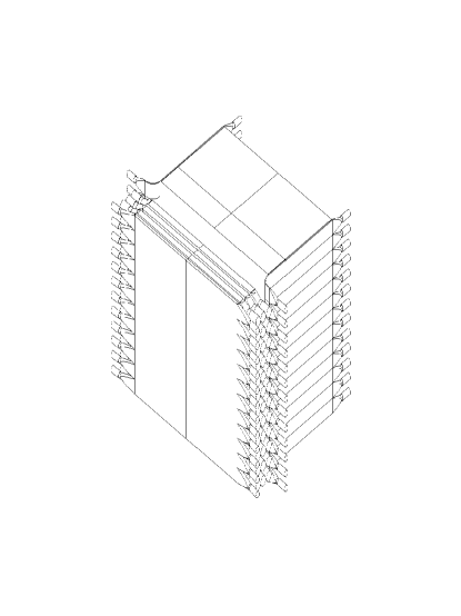
FIG. 4.: Isometric view of E789 electromagnetic and hadronic calorimeters.

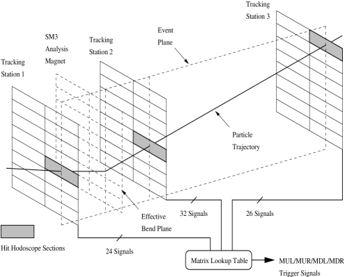
FIG. 5.: Conceptual sketch of hodoscope trigger matrix.

FIG. 6.: Distance between the downstream track and the associated SSD hit for the Y planes in the lower SSD arm for events with only one SSD track in either arm.

FIG. 7.: $y$- and $x$-angle matching between downstream track and SSD track for both SSD arms for events with only one SSD track in either arm.

FIG. 8.: Monte-Carlo generated (left) and accepted (right) distributions of $p_{t}$, $x_{F}$ and z component of momentum in the laboratory frame for $D^{0}$ with SM12 set at 900 A.

FIG. 9.: Trigger efficiency for dihadron events as a function of pair momentum. The solid curve is the parametrization used in the Monte Carlo program.

FIG. 10.: Efficiency of dielectron trigger as a function of Monte-Carlo generated $D^{0}$ momentum. This efficiency was used for both 900A and 1000A runs.

FIG. 11.: Efficiency of single-electron trigger as a function of Monte-Carlo generated $D^{0}$ momentum. This efficiency was used for analyzing the 900A and 1000A data.

FIG. 12.: Reconstructed $K\pi$ invariant-mass distribution of Monte-Carlo ${D^{0}\ {\rightarrow}\ K\pi}$ events at 900 A, with entries both for correct and for incorrect particle assignments.

FIG. 13.: Invariant mass distributions for ${D^{0}\ {\rightarrow}\ \mu^{+}\mu^{-}}$ and its associated ${D^{0}\ {\rightarrow}\ K\pi}$ distribution for the 900A-Au and dedicated-dilepton data sets. The cross-hatched area marks the signal region.

FIG. 14.: Invariant mass distribution for ${D^{0}\ {\rightarrow}\ \mu^{+}\mu^{-}}$ and its associated ${D^{0}\ {\rightarrow}\ K\pi}$ distribution for the 1000A-Au and 900A-Be data sets. The cross-hatched area marks the signal region.

FIG. 15.: Invariant mass distribution for ${D^{0}\ {\rightarrow}\ e^{+}e^{-}}$ and its associated ${D^{0}\ {\rightarrow}\ K\pi}$ distribution for the 900A-Au and dedicated-dilepton data sets. The cross-hatched area marks the signal region.

FIG. 16.: Invariant-mass distribution for ${D^{0}\ {\rightarrow}\ e^{+}e^{-}}$ and its associated ${D^{0}\ {\rightarrow}\ K\pi}$ distribution for the 1000A-Au and 900A-Be data sets. The cross-hatched area marks the signal region.

FIG. 17.: Invariant mass distribution for ${D^{0}\ {\rightarrow}\ \mu^{\pm}e^{\mp}}$ and its associated ${D^{0}\ {\rightarrow}\ K\pi}$ distribution for the 900A-Au and dedicated-dilepton data sets. The cross-hatched area marks the signal regions.

FIG. 18.: Invariant mass distribution for ${D^{0}\ {\rightarrow}\ \mu^{\pm}e^{\mp}}$ and its associated ${D^{0}\ {\rightarrow}\ K\pi}$ distribution for the 1000A-Au and 900A-Be data sets. The cross-hatched area marks the signal region.

TABLE I.: Dimensions of targets.

	$900$A	$1000$A
Length along $z$ (mm)	1.8	0.8
Height along $y$ ($\mu$m)	160	110

TABLE II.: Configuration of Silicon Vertex Detector.

Plane		$z$ Position	$y$ Position			Number
No.	Name	(cm)	(cm)	View	Arm	of Strips
1	Y1B	-294.54	-2.125	Y	Lower	316
2	Y1T	-291.36	0.949	Y	Upper	316
3	U2B	-286.92	-2.300	U	Lower	372
4	U2T	-283.74	1.066	U	Upper	372
5	Y3B	-279.30	-2.758	Y	Lower	436
6	Y3T	-276.12	1.548	Y	Upper	436
7	V4B	-271.68	-2.865	V	Lower	500
8	V4T	-268.50	1.721	V	Upper	500
9	Y5B	-264.07	-3.364	Y	Lower	572
10	Y5T	-260.88	2.217	Y	Upper	572
11	U6B	-256.44	-3.566	U	Lower	628
12	U6T	-253.26	2.289	U	Upper	628
13	Y7B	-248.82	-4.018	Y	Lower	692
14	Y7T	-245.64	2.805	Y	Upper	692
15	V8B	-241.20	-4.154	V	Lower	756
16	V8T	-238.02	2.925	V	Upper	756

TABLE III.: Components of TGO Trigger.

Trigger Name	Description
${\it h}^{+}{\it h}^{-}$	${\it M_{U}}\cdot{\it M_{D}}\cdot{\it S_{U}}\cdot{\it S_{D}}\cdot{\overline{\it NX1}}\cdot{\overline{\it NX3}}\cdot{\it H}$
${\mu}^{+}{\mu}^{-}$	${\it M_{U}}\cdot{\it M_{D}}\cdot{\it S_{U}}\cdot{\it S_{D}}\cdot{\overline{\it NX1}}\cdot{\overline{\it NX3}}\cdot 2{\it HX4}\cdot 2{\it HY4}$
${\it e}^{+}{\it e}^{-}$	${\it M_{U}}\cdot{\it M_{D}}\cdot{\it S_{U}}\cdot{\it S_{D}}\cdot{\overline{\it NX1}}\cdot{\overline{\it NX3}}\cdot{\it E}$
${\it e}^{\mp}{\mu}^{\pm}$	${\it M_{U}}\cdot{\it M_{D}}\cdot{\it S_{U}}\cdot{\it S_{D}}\cdot{\overline{\it NX1}}\cdot{\overline{\it NX3}}\cdot{\it e}\cdot{\it HX4}\cdot{\it HY4}$
${\it h}^{\mp}{\it e}^{\pm}$	${\it M_{U}}\cdot{\it M_{D}}\cdot{\it S_{U}}\cdot{\it S_{D}}\cdot{\overline{\it NX1}}\cdot{\overline{\it NX3}}\cdot{\it h}\cdot{\it e}$
${\it h}^{\mp}{\mu}^{\pm}$	${\it M_{U}}\cdot{\it M_{D}}\cdot{\it S_{U}}\cdot{\it S_{D}}\cdot{\overline{\it NX1}}\cdot{\overline{\it NX3}}\cdot{\it h}\cdot{\it HX4}\cdot{\it HY4}$
${\it h}^{\pm}{\it h}^{\pm}$	${\it M_{LIKE}}\cdot({\it S_{U}}+{\it S_{D}})\cdot{\overline{\it NX1}}\cdot{\overline{\it NX3}}\cdot{\it H}$
${\mu}^{\pm}{\mu}^{\pm}$	${\it M_{LIKE}}\cdot({\it S_{U}}+{\it S_{D}})\cdot{\overline{\it NX1}}\cdot{\overline{\it NX3}}\cdot 2{\it HX4}\cdot 2{\it HY4}$
${\it e}^{\pm}{\it e}^{\pm}$	${\it M_{LIKE}}\cdot({\it S_{U}}+{\it S_{D}})\cdot{\overline{\it NX1}}\cdot{\overline{\it NX3}}\cdot{\it E}$
${\it e}^{\pm}{\mu}^{\pm}$	${\it M_{LIKE}}\cdot({\it S_{U}}+{\it S_{D}})\cdot{\overline{\it NX1}}\cdot{\overline{\it NX3}}\cdot{\it e}\cdot{\it HX4}\cdot{\it HY4}$
${\it h}^{\pm}{\it e}^{\pm}$	${\it M_{LIKE}}\cdot({\it S_{U}}+{\it S_{D}})\cdot{\overline{\it NX1}}\cdot{\overline{\it NX3}}\cdot{\it h}\cdot{\it e}$
${\it h}^{\pm}{\mu}^{\pm}$	${\it M_{LIKE}}\cdot({\it S_{U}}+{\it S_{D}})\cdot{\overline{\it NX1}}\cdot{\overline{\it NX3}}\cdot{\it h}\cdot{\it HX4}\cdot{\it HY4}$

TABLE IV.: Average number of protons on target and triggers per 23-sec spill.

Run	Protons on Target	TFI	TGO	TAP
900A-Be	$3.6\times 10^{10}$	$2.8\times 10^{6}$	$1.7\times 10^{5}$	$8.7\times 10^{3}$
900A-Au	$3.3\times 10^{10}$	$8.3\times 10^{6}$	$1.0\times 10^{5}$	$2.2\times 10^{4}$
1000A-Au	$2.6\times 10^{10}$	$1.7\times 10^{6}$	$1.0\times 10^{5}$	$2.6\times 10^{4}$

TABLE V.: Summary of data sets.

Data set	Protons on target	$AMON\cdot\overline{SB}$	TAPS
1000A-Au	$7.2\times 10^{13}$	$3.9\times 10^{6}$	$3.8\times 10^{8}$
900A-Au	$1.2\times 10^{13}$	$8.4\times 10^{5}$	$8.7\times 10^{7}$
900A-Au-Dedicated-Dilepton	$6.6\times 10^{13}$	$3.4\times 10^{6}$	$7.0\times 10^{7}$
900A-Be	$2.2\times 10^{14}$	$9.8\times 10^{5}$	$7.3\times 10^{7}$

TABLE VI.: Lifetime Significance and impact parameter cuts for ${D^{0}\ {\rightarrow}\ \mu^{+}\mu^{-}}$.

	900A-Au	900A-Au-Dedicated-Dilepton	900A-Be	1000A-Au
Lifetime Significance	1.0	0.60	0.90	1.4
Impact Parameter ($\mu$m)	25.4	109	78.7	95.3

TABLE VII.: Lifetime Significance and impact parameter cuts for ${D^{0}\ {\rightarrow}\ e^{+}e^{-}}$.

	900A-Au	900A-Au-Dedicated-Dilepton	900A-Be	1000A-Au
Lifetime Significance	0.80	0.90	0.60	0.80
Impact Parameter ($\mu$m)	48.3	82.6	29.2	55.9

TABLE VIII.: Lifetime Significance and impact parameter cuts for ${D^{0}\ {\rightarrow}\ \mu^{\pm}e^{\mp}}$.

	900A-Au	900A-Au-Dedicated-Dilepton	900A-Be	1000A-Au
Lifetime Significance	1.5	1.3	1.0	1.4
Impact Parameter ($\mu$m)	190.	97.8	90.2	55.9

TABLE IX.: Parameters of ${D^{0}\ {\rightarrow}\ K\pi}$ normalization for ${D^{0}\ {\rightarrow}\ \mu^{+}\mu^{-}}$ search.

Data set	900A-Au	900A-Be	1000A-Au	Dilepton
Mean Mass (GeV/$c^{2}$)	1.865	1.863	1.867	1.866
Mass Resolution, $\sigma$ (MeV/$c^{2}$)	7.0	5.6	7.3	7.9
Total # of ${D^{0}\ {\rightarrow}\ K\pi}$ decays	$606\pm 56$	$1161\pm 110$	$971\pm 57$	$2794\pm 396$

TABLE X.: Parameters of ${D^{0}\ {\rightarrow}\ K\pi}$ normalization for ${D^{0}\ {\rightarrow}\ e^{+}e^{-}}$ search.

Data set	900A-Au	900A-Be	1000A-Au	Dilepton
Mean Mass (GeV/$c^{2}$)	1.865	1.863	1.866	1.865
Mass Resolution, $\sigma$ (MeV/$c^{2}$)	6.1	5.9	6.5	6.2
Total # of ${D^{0}\ {\rightarrow}\ K\pi}$ decays	$707\pm 91$	$1563\pm 154$	$1749\pm 129$	$2867\pm 466$

TABLE XI.: Parameters of ${D^{0}\ {\rightarrow}\ K\pi}$ normalization for ${D^{0}\ {\rightarrow}\ \mu^{\pm}e^{\mp}}$ search.

Data set	900A-Au	900A-Be	1000A-Au	Dilepton
Mean Mass (GeV/$c^{2}$)	1.865	1.864	1.867	1.865
Mass Resolution, $\sigma$ (MeV/$c^{2}$)	6.0	6.5	7.1	6.3
Total # of ${D^{0}\ {\rightarrow}\ K\pi}$ decays	$255\pm 21$	$967\pm 62$	$1429\pm 84$	$2400\pm 337$

TABLE XII.: Width of invariant-mass distribution for reconstructed dilepton events relative to that of the normalization signal, as determined by Monte Carlo.

	${D^{0}\ {\rightarrow}\ \mu^{+}\mu^{-}}$	${D^{0}\ {\rightarrow}\ e^{+}e^{-}}$	${D^{0}\ {\rightarrow}\ \mu^{\pm}e^{\mp}}$
900A	1.08	1.09	1.08
1000A	1.09	1.08	1.07

TABLE XIII.: Efficiencies for ${D^{0}\ {\rightarrow}\ K\pi}$ decay.

	900A	1000A
Geometric	$(3.55\pm 0.02)\times 10^{-3}$	$(2.37\pm 0.01)\times 10^{-3}$
K decays	$0.78\pm 0.01$	$0.82\pm 0.01$
Trigger	$0.55\pm 0.01$	$0.58\pm 0.01$
Final cuts	$(7.12\pm 0.04)\times 10^{-2}$	$(9.35\pm 0.05)\times 10^{-2}$
Total	$(1.08\pm 0.02)\times 10^{-4}$	$(1.05\pm 0.02)\times 10^{-4}$

TABLE XIV.: Efficiencies for ${D^{0}\ {\rightarrow}\ \mu^{+}\mu^{-}}$ decay.

	900A	1000A
Geometric	$(3.97\pm 0.02)\times 10^{-3}$	$(3.05\pm 0.02)\times 10^{-3}$
Trigger $\cdot$ ID $\cdot$ isolation	$0.36\pm 0.01$	$0.50\pm 0.01$
Final cuts	$(7.30\pm 0.04)\times 10^{-2}$	$(9.85\pm 0.05)\times 10^{-2}$
Total	$(1.05\pm 0.02)\times 10^{-4}$	$(1.51\pm 0.02)\times 10^{-4}$

TABLE XV.: Efficiencies for ${D^{0}\ {\rightarrow}\ e^{+}e^{-}}$ decay.

	900A	1000A
Geometric	$(3.87\pm 0.02)\times 10^{-3}$	$(3.28\pm 0.02)\times 10^{-3}$
Trigger $\cdot$ ID	$0.60\pm 0.01$	$0.60\pm 0.01$
Final cuts	$(7.15\pm 0.04)\times 10^{-2}$	$(10.0\pm 0.05)\times 10^{-2}$
Total	$(1.65\pm 0.03)\times 10^{-4}$	$(1.98\pm 0.04)\times 10^{-4}$

TABLE XVI.: Efficiencies for ${D^{0}\ {\rightarrow}\ \mu^{\pm}e^{\mp}}$ decay.

	900A	1000A
Geometric	$(4.18\pm 0.02)\times 10^{-3}$	$(3.42\pm 0.02)\times 10^{-3}$
Trigger $\cdot$ ID	$0.36\pm 0.01$	$0.36\pm 0.01$
Final cuts	$(7.04\pm 0.04)\times 10^{-2}$	$(10.0\pm 0.05)\times 10^{-2}$
Total	$(1.06\pm 0.03)\times 10^{-4}$	$(1.28\pm 0.04)\times 10^{-4}$

TABLE XVII.: Summary of results.

Decay	$\sum_{i}N_{i}\epsilon_{i}$	Single-event	Limit from MC	Cousins-Feldman
Mode		Sensitivity	calculation	Method
${D^{0}\ {\rightarrow}\ \mu^{+}\mu^{-}}$	5830	7.34 $\times 10^{-6}$	1.56 $\times 10^{-5}$	1.65 $\times 10^{-5}$
${D^{0}\ {\rightarrow}\ e^{+}e^{-}}$	11100	3.84 $\times 10^{-6}$	0.82 $\times 10^{-5}$	0.87 $\times 10^{-5}$
${D^{0}\ {\rightarrow}\ \mu^{\pm}e^{\mp}}$	5300	8.08 $\times 10^{-6}$	1.72 $\times 10^{-5}$	1.82 $\times 10^{-5}$

REFERENCES

- [1] Present Address: Kellogg Laboratory, California Institute of Technology, Pasadena, California 91125.
- [2] Present Address: Visa International, 3055 Clearview Way, MS 3A, San Mateo, California 94402.
- [3] Present Address: Stanford Research Systems, 1290 D Reamwood Avenue, Sunnyvale, CA 94089.
- [4] Present Address: Department of Physics, Purdue University, Lafayette, Indiana 47907.
- [5] Present Address: Department of Physics, Illinois Institute of Technology, Chicago, Illinois 60616.
- [6] Present Address: Cypress Semiconductor, Minneapolis, Minnesota 55455.
- [7] Present Address: Department of Physics, University of California, Riverside, California 92521.
- [8] Present Address: Max-Planck-Institut fur Kernphysik, Heidelberg, Germany.
- [9] Present Address: Science Applications International Corp., 2950 Patrick Henry Dr., Santa Clara, CA 95054.
- [10] Present Address: Department of Physics, Iowa State University, Ames, Iowa 50011-3160.
- [11] Present Address: Institute of Physics, Academia Sinica, Taipei, Taiwan.
- [12] W. Buchmuller and D. Wyler, Phys. Lett. 177B, 377 (1986).
- [13] K.S. Babu, X.G. He, X. Li, and S. Pakvasa, Phys. Lett. 205B, 540 (1988).
- [14] S. Pakvasa, Chin. J. Phys. 32, 1163 (1994), hep-ph/9408270.
- [15] CLEO, A. Freyberger et al., Phys. Rev. Lett. 76, 3065 (1996); Erratum, Phys. Rev. Lett. 77, 2147 (1996).
- [16] M. Adamovich et al., Phys. Lett. B408, 469 (1997).
- [17] E771, T. Alexopoulos et al., Phys. Rev. Lett. 77, 2380 (1996).
- [18] Y.-C. Chen, PhD thesis, National Cheng Kung University, 1993.
- [19] R.J. Yarema, T. Zimmerman, IEEE Trans. Nucl. Sci. NS37, 430 (1990); T. Zimmerman, IEEE Trans. Nucl. Sci. NS37, 439 (1990).
- [20] B.T. Turko et al., IEEE Trans. Nucl. Sci. NS39, 758 (1992).
- [21] Designed by J.A. Crittenden and D.M. Kaplan, Columbia University Nevis Laboratories (1984), after a ca.-1970 design by F.W. Sippach.
- [22] A. Ito et al., Fermilab-TM-1200 (1983).
- [23] Designed by D.M. Kaplan, Columbia University Nevis Laboratories (1982).
- [24] D. Pripstein, PhD thesis, University of California at Berkeley, 1998.
- [25] J.A. Crittenden et al., IEEE Trans. Nucl. Sci. NS31, 1028 (1984).
- [26] W. Sippach et al., IEEE Trans. Nucl. Sci. NS27, 578 (1980).
- [27] M.H. Schub et al., Nucl. Instrum. Meth. A376, 49 (1996).
- [28] M.J. Leitch et al., Phys. Rev. Lett. 72, 2542 (1994).
- [29] Particle Data Group, Phys. Rev. D54 (1996).
- [30] Fermilab E653, K. Kodama et al., Phys. Lett. B263, 573 (1991).
- [31] C. Peterson, T. Rognvaldsson, and L. Lonnblad, Comp. Phys. Comm. 81, 185 (1994).
- [32] F. James et al., CERN Program Library Long Writeup D506, MINUIT Release 94.09 (1994).
- [33] R. Brun et al., CERN Program Library Q121, PAW version 2.05/17 (1994).
- [34] G.J. Feldman and R.D. Cousins, Phys. Rev. D57, 3873 (1998).
- [35] C. Caso et al., Eur. Phys. J. C3,174 (1998).
- [36] R.D. Cousins and V.L. Highland, Nucl. Instr. Meth. A320, 331 (1992).