Measurement of $B\rightarrow\rho\ell\nu$ decay and $|V_{ub}|$

Abstract

Using a sample of $3.3\times 10^{6}$ $\Upsilon(4S)\rightarrow B\bar{B}$ events collected with the CLEO II detector at the Cornell Electron Storage Ring (CESR), we measure ${\cal B}(B\rightarrow\rho\ell\nu)$, $|V_{ub}|$, and the partial rate ($\Delta\Gamma$) in three bins of $q^{2}\equiv(p_{B}-p_{\rho})^{2}$. We find ${\cal B}(B^{0}\rightarrow\rho^{-}\ell^{+}\nu)=(2.69\pm 0.41^{+0.35}_{-0.40}\pm 0.50)\times 10^{-4}$, $|V_{ub}|=(3.23\pm 0.24^{+0.23}_{-0.26}\pm 0.58)\times 10^{-3}$, $\Delta\Gamma(0<q^{2}<7~{}{\rm GeV}^{2}/c^{4})=(7.6\pm 3.0^{+0.9}_{-1.2}\pm 3.0)\times 10^{-2}~{}{\rm ns}^{-1}$, $\Delta\Gamma(7<q^{2}<14~{}{\rm GeV}^{2}/c^{4})=(4.8\pm 2.9^{+0.7}_{-0.8}\pm 0.7)\times 10^{-2}~{}{\rm ns}^{-1}$, and $\Delta\Gamma(14<q^{2}<21~{}{\rm GeV}^{2}/c^{4})=(7.1\pm 2.1^{+0.9}_{-1.1}\pm 0.6)\times 10^{-2}~{}{\rm ns}^{-1}$. T Here, $\ell=e$ or $\mu$, but not both, and the quoted errors are statistical, systematic, and theoretical. The method is sensitive primarily to $B\rightarrow\rho\ell\nu$ decays with leptons in the energy range above 2.3 GeV. Averaging with the previously published CLEO results for $B\rightarrow\rho\ell\nu$, we obtain ${\cal B}(B^{0}\rightarrow\rho^{-}\ell^{+}\nu)=(2.57\pm 0.29^{+0.33}_{-0.46}\pm 0.41)\times 10^{-4}$ and $|V_{ub}|=(3.25\pm 0.14^{+0.21}_{-0.29}\pm 0.55)\times 10^{-3}$.

B. H. Behrens,¹ W. T. Ford,¹ A. Gritsan,¹ H. Krieg,¹ J. Roy,¹ J. G. Smith,¹ J. P. Alexander,² R. Baker,² C. Bebek,² B. E. Berger,² K. Berkelman,² V. Boisvert,² D. G. Cassel,² D. S. Crowcroft,² M. Dickson,² S. von Dombrowski,² P. S. Drell,² K. M. Ecklund,² R. Ehrlich,² A. D. Foland,² P. Gaidarev,² L. Gibbons,² B. Gittelman,² S. W. Gray,² D. L. Hartill,² B. K. Heltsley,² P. I. Hopman,² D. L. Kreinick,² T. Lee,² Y. Liu,² T. 0. Meyer,² N. B. Mistry,² C. R. Ng,² E. Nordberg,² M. Ogg,^2, J. R. Patterson,² D. Peterson,² D. Riley,² J. G. Thayer,² P. G. Thies,² B. Valant-Spaight,² A. Warburton,² C. Ward,² M. Athanas,³ P. Avery,³ C. D. Jones,³ M. Lohner,³ C. Prescott,³ A. I. Rubiera,³ J. Yelton,³ J. Zheng,³ G. Brandenburg,⁴ R. A. Briere,⁴ A. Ershov,⁴ Y. S. Gao,⁴ D. Y.-J. Kim,⁴ R. Wilson,⁴ T. E. Browder,⁵ Y. Li,⁵ J. L. Rodriguez,⁵ H. Yamamoto,⁵ T. Bergfeld,⁶ B. I. Eisenstein,⁶ J. Ernst,⁶ G. E. Gladding,⁶ G. D. Gollin,⁶ R. M. Hans,⁶ E. Johnson,⁶ I. Karliner,⁶ M. A. Marsh,⁶ M. Palmer,⁶ C. Plager,⁶ C. Sedlack,⁶ M. Selen,⁶ J. J. Thaler,⁶ J. Williams,⁶ K. W. Edwards,⁷ A. Bellerive,⁸ R. Janicek,⁸ P. M. Patel,⁸ A. J. Sadoff,⁹ R. Ammar,¹⁰ P. Baringer,¹⁰ A. Bean,¹⁰ D. Besson,¹⁰ D. Coppage,¹⁰ R. Davis,¹⁰ S. Kotov,¹⁰ I. Kravchenko,¹⁰ N. Kwak,¹⁰ X. Zhao,¹⁰ L. Zhou,¹⁰ S. Anderson,¹¹ V. V. Frolov,¹¹ Y. Kubota,¹¹ S. J. Lee,¹¹ R. Mahapatra,¹¹ J. J. O’Neill,¹¹ R. Poling,¹¹ T. Riehle,¹¹ A. Smith,¹¹ M. S. Alam,¹² S. B. Athar,¹² A. H. Mahmood,¹² S. Timm,¹² F. Wappler,¹² A. Anastassov,¹³ J. E. Duboscq,¹³ K. K. Gan,¹³ C. Gwon,¹³ T. Hart,¹³ K. Honscheid,¹³ H. Kagan,¹³ R. Kass,¹³ J. Lorenc,¹³ H. Schwarthoff,¹³ E. von Toerne,¹³ M. M. Zoeller,¹³ S. J. Richichi,¹⁴ H. Severini,¹⁴ P. Skubic,¹⁴ A. Undrus,¹⁴ M. Bishai,¹⁵ S. Chen,¹⁵ J. Fast,¹⁵ J. W. Hinson,¹⁵ J. Lee,¹⁵ N. Menon,¹⁵ D. H. Miller,¹⁵ E. I. Shibata,¹⁵ I. P. J. Shipsey,¹⁵ S. Glenn,¹⁶ Y. Kwon,^16, A.L. Lyon,¹⁶ E. H. Thorndike,¹⁶ C. P. Jessop,¹⁷ K. Lingel,¹⁷ H. Marsiske,¹⁷ M. L. Perl,¹⁷ V. Savinov,¹⁷ D. Ugolini,¹⁷ X. Zhou,¹⁷ T. E. Coan,¹⁸ V. Fadeyev,¹⁸ I. Korolkov,¹⁸ Y. Maravin,¹⁸ I. Narsky,¹⁸ R. Stroynowski,¹⁸ J. Ye,¹⁸ T. Wlodek,¹⁸ M. Artuso,¹⁹ S. Ayad,¹⁹ E. Dambasuren,¹⁹ S. Kopp,¹⁹ G. Majumder,¹⁹ G. C. Moneti,¹⁹ R. Mountain,¹⁹ S. Schuh,¹⁹ T. Skwarnicki,¹⁹ S. Stone,¹⁹ A. Titov,¹⁹ G. Viehhauser,¹⁹ J.C. Wang,¹⁹ S. E. Csorna,²⁰ K. W. McLean,²⁰ S. Marka,²⁰ Z. Xu,²⁰ R. Godang,²¹ K. Kinoshita,^21, I. C. Lai,²¹ P. Pomianowski,²¹ S. Schrenk,²¹ G. Bonvicini,²² D. Cinabro,²² R. Greene,²² L. P. Perera,²² G. J. Zhou,²² S. Chan,²³ G. Eigen,²³ E. Lipeles,²³ M. Schmidtler,²³ A. Shapiro,²³ W. M. Sun,²³ J. Urheim,²³ A. J. Weinstein,²³ F. Würthwein,²³ D. E. Jaffe,²⁴ G. Masek,²⁴ H. P. Paar,²⁴ E. M. Potter,²⁴ S. Prell,²⁴ V. Sharma,²⁴ D. M. Asner,²⁵ A. Eppich,²⁵ J. Gronberg,²⁵ T. S. Hill,²⁵ D. J. Lange,²⁵ R. J. Morrison,²⁵ H. N. Nelson,²⁵ T. K. Nelson,²⁵ J. D. Richman,²⁵ and D. Roberts²⁵

I Introduction

Exclusive semileptonic $b\rightarrow u\ell\nu$ decays are an active area of experimental and theoretical study [1, 2, 3, 4, 5, 6, 7, 8, 9, 10, 11, 12, 13, 14, 15, 16, 17, 18, 19, 20, 21, 22, 23]. These rare processes can be used to extract the magnitude of $V_{ub}$, one of the smallest and least well known elements of the Cabibbo-Kobayashi-Maskawa (CKM) quark-mixing matrix [24]. Because $|V_{ub}/V_{cb}|\approx 0.08$, the branching fractions for exclusive $b\rightarrow u\ell\nu$ processes are small, of order $10^{-4}$, and they have only recently become experimentally accessible. The present analysis confirms the initial CLEO observation [1] of $B\rightarrow\rho\ell\nu$, improves the precision on the branching fraction and $|V_{ub}|$, and provides the first information on the $q^{2}$ dependence for this decay.

Extracting $|V_{ub}|$ from a measured decay rate requires significant theoretical input because the matrix elements for such processes involve complex strong-interaction dynamics. Although the underlying $b\to u\ell\nu$ decay is a relatively simple weak process, it is difficult to calculate the strong-interaction effects involved in the transition from the heavy $B$ meson to the light daughter meson. Because of these theoretical uncertainties, even a perfectly measured $B\to\rho\ell\nu$ branching fraction would not at present lead to a precise value of $|V_{ub}|$.

The dynamics in $B\to\rho\ell\nu$ decay are in contrast with $b\to c\ell\nu$ decays, such as $B\to D^{*}\ell\nu$, where a heavy quark is present both in initial and final states. In this case, techniques based on Heavy Quark Effective Theory (HQET) can be used to calculate the decay amplitude with good precision, particularly for the kinematic configuration in which the charm hadron has zero recoil velocity. The zero-recoil point in $B\to\rho\ell\nu$ cannot be treated with similar techniques, however, because the daughter $u$ quark is not heavy compared to the scale of hadronic energy transfers. Nevertheless, substantial progress has been made using a variety of theoretical methods, including quark models [6, 7, 8, 9, 10, 11, 12], lattice QCD [13, 14, 15], QCD sum rules [16, 17, 18], and models relating form factors measured in $D\rightarrow K^{*}\ell\nu$ decay [19] to those in $B\to\rho\ell\nu$ decay.

Experimentally, the main difficulty in observing signals from $b\to u\ell\nu$ processes is the very large background due to $b\to c\ell\nu$. Because a significant fraction of $B\to\rho\ell\nu$ events have lepton energy beyond the endpoint for $b\to c\ell\nu$ decay, lepton-energy requirements provide a powerful tool for background suppression. However, extrapolation of the decay rate measured in this portion of phase space to the full rate again requires the use of theoretical models, and it introduces model dependence beyond that associated with simply extracting the value of $|V_{ub}|$ from the branching fraction. In this study, we begin to explore the decay dynamics of $B\to\rho\ell\nu$ by measuring the distribution of $q^{2}$, the square of the mass of the virtual $W$. The distribution of $q^{2}$ is reflected in the $\rho$ momentum spectrum. Eventually, studies of the $q^{2}$ distribution, as well as of the angular distributions of the decay products, should reduce the model dependence on $|V_{ub}|$ by constraining theoretical models for the decay form factors.

CLEO has previously observed [1] the decays $B^{0}\rightarrow\rho^{-}\ell^{+}\nu$, $B^{+}\rightarrow\rho^{0}\ell^{+}\nu$, $B^{0}\rightarrow\pi^{-}\ell^{+}\nu$, and $B^{+}\rightarrow\pi^{0}\ell^{+}\nu$ by measuring both the missing energy and momentum in an event to infer the momentum of the neutrino. Using $2.84\times 10^{6}$ $\Upsilon(4S)\to B\bar{B}$ events, this study obtained

$${\cal B}(B^{0}\rightarrow\rho^{-}\ell^{+}\nu) = (2.5\pm 0.4^{+0.5}_{-0.7}\pm 0.5)\times 10^{-4},$$ (1)

$${\cal B}(B^{0}\rightarrow\pi^{-}\ell^{+}\nu) = (1.8\pm 0.4\pm 0.3\pm 0.2)\times 10^{-4},$$ (2)

$$|V_{ub}| = (3.3\pm 0.2^{+0.3}_{-0.4}\pm 0.7)\times 10^{-3},$$ (3)

where the errors are statistical, systematic, and theoretical. A large contribution to the $B\rightarrow\rho\ell\nu$ systematic error is associated with a possible nonresonant $B\rightarrow\pi\pi\ell\nu$ rate. In the analysis described below this uncertainty is reduced.

We report on a measurement of ${\cal B}(B\rightarrow\rho\ell\nu)$ and $|V_{ub}|$ as well as the first measurement of the partial rate for $B\rightarrow\rho\ell\nu$ in bins of $q^{2}$. We study five signal modes: $B^{0}\to\rho^{-}\ell^{+}\nu$, $B^{+}\to\rho^{0}\ell^{+}\nu$, $B^{+}\to\omega\ell^{+}\nu$, $B^{0}\to\pi^{-}\ell^{+}\nu$, and $B^{+}\to\pi^{0}\ell^{+}\nu$. Our method is sensitive primarily to leptons with energies above the $b\rightarrow c\ell\nu$ lepton-energy endpoint ($E_{\ell}>2.3~{}{\rm GeV}$). The resulting event sample is essentially statistically independent of that from the previous analysis since it contains much larger signal and background yields, even though the data samples are similar.

In this paper, we use the notation $b\to u(c)\ell\nu$ to denote inclusive $B\to X_{u(c)}\ell\nu$ decay, where $X_{u}$ is a hadronic system with no charm quarks, and $X_{c}$ is a hadronic system with a charm quark. When discussing backgrounds, we will often refer to $b\to u\ell\nu$ inclusive decays excluding one or more signal modes. In this case, we will use the notation $b\to u\ell\nu$ and explicitly list the modes not to be included. When no charge state is given, $B\to\rho\ell\nu$ refers generically to $B\to\rho^{\pm}\ell\nu$, and $B\to\rho^{0}\ell\nu$ decays. When specifying a particular decay mode, we implicitly include its charge-conjugate decay.

We begin in Sec. II by introducing the phenomenology of $B\rightarrow\rho\ell\nu$ decay. The full differential decay rate is expressed in terms of helicity amplitudes, which depend in turn on form factors, Lorentz-invariant functions of $q^{2}$ that parametrize the hadronic current. We discuss five form-factor models that are used to obtain $|V_{ub}|$ and to extrapolate our yield measured at high lepton energy to the full phase space available in $B\rightarrow\rho\ell\nu$ decay.

Section III describes the data sample and the requirements used to distinguish signal events from backgrounds, which are due primarily to continuum events ($e^{+}e^{-}\to q\bar{q}$, $q\bar{q}=u\bar{u}$, $d\bar{d}$, $s\bar{s}$, and $c\bar{c}$), $b\rightarrow c\ell\nu$, and $b\rightarrow u\ell\nu$ (other than $B\to\rho\ell\nu$ or $B\to\omega\ell\nu$) events.

Section IV describes the binned maximum-likelihood fit used to extract the $B\rightarrow\rho\ell\nu$ signal. Although we must rely on Monte Carlo calculations to model the shapes of distributions for the $b\rightarrow c(u)\ell\nu$ backgrounds, the normalization and lepton-energy spectrum of each background component are determined by the data. In addition, the assumed background shapes are extensively tested using sideband regions where the contribution from signal events is small. The continuum background contribution is measured directly using data. Section V presents the yields extracted from the fit and the model-dependent detection efficiencies used to obtain values for ${\cal B}(B\rightarrow\rho\ell\nu)$ and $|V_{ub}|$.

Section VI describes the contributions to our systematic error. Apart from model dependence, these are due primarily to uncertainties in the $b\rightarrow u\ell\nu$ backgrounds and to uncertainties in the detector simulation. In the high lepton-energy region, where the sensitivity to the signal is greatest, the background from other $b\to u\ell\nu$ processes is comparable to that from $b\to c\ell\nu$ decays, but its kinematic properties are less well understood.

Section VII presents our measured values of ${\cal B}(B\to\rho\ell\nu)$ and $|V_{ub}|$, as well as the average with the previous CLEO result. This average takes into account the correlation in the systematic errors as well as the variation in results for different form-factor models. In Sec. VIII we present our conclusions and an outlook for future measurements.

II Semileptonic decay kinematics

The matrix element for the semileptonic decay $P(Q\bar{q})\rightarrow V(q^{\prime}\bar{q})\ell^{-}\bar{\nu}$ of a pseudoscalar meson, $P(Q\bar{q})$, to a vector meson, $V(q^{\prime}\bar{q})$, can be written [25]

$${\cal M}(P\rightarrow V\ell\nu)=-{\it i}{{G_{F}}\over{\sqrt{2}}}V_{q^{\prime}Q}L^{\mu}J_{\mu},$$ (4)

where $V_{q^{\prime}Q}$ is the CKM matrix element for the $Q\to q^{\prime}$ transition [26], $L^{\mu}$ is the leptonic current

$$L^{\mu}=\bar{u}_{\ell}\gamma^{\mu}(1-\gamma_{5})v_{\nu},$$ (5)

and the hadronic current

$$J_{\mu}=\left<V(p_{V},\varepsilon)|(V-A)_{\mu}|P(p_{P})\right>= - \varepsilon^{*}_{\mu}(m_{P}+m_{V})A_{1}(q^{2})$$ (6)

$$+ (p_{V}+p_{P})_{\mu}(\varepsilon^{*}\cdot q){{A_{2}(q^{2})}\over{(m_{P}+m_{V})}}$$ (7)

$$+ q_{\mu}(\varepsilon^{*}\cdot q){{2m_{V}}\over{q^{2}}}\bigl{(}A_{3}(q^{2})-A_{0}(q^{2})\bigr{)}$$ (8)

$$+ 2i\epsilon_{\mu\nu\rho\sigma}\varepsilon^{*\nu}p_{V}^{\rho}p_{P}^{\sigma}{{{V}(q^{2})}\over{m_{P}+m_{V}}},$$ (9)

is written in terms of four form factors, $A_{1}(q^{2})$, $A_{2}(q^{2})$, $V(q^{2})$, and $A_{0}(q^{2})$, where $A_{0}(0)=A_{3}(0)$ and

$$A_{3}(q^{2})={{m_{P}+m_{V}}\over{2m_{V}}}A_{1}(q^{2})-{{m_{P}-m_{V}}\over{2m_{V}}}A_{2}(q^{2}).$$ (10)

Here $m_{P}$, $m_{V}$, $p_{P}$, and $p_{V}$ are the pseudoscalar and vector meson masses and four-momenta, $q\equiv p_{P}-p_{V}$, and $\varepsilon$ is the vector-meson polarization four-vector. Terms in $J_{\mu}$ proportional to $q_{\mu}$ vanish in the limit of massless leptons, so that the decay $B\rightarrow\rho\ell\nu$ depends effectively on only three form factors ($A_{1}(q^{2})$, $A_{2}(q^{2})$, and $V(q^{2})$) for electrons or muons.

The amplitudes for the vector meson to have helicity $+1$, $-1$, or $0$, denoted by $H_{+}(q^{2})$, $H_{-}(q^{2})$, and $H_{0}(q^{2})$, can be expressed in terms of the form factors:

$$H_{\pm}(q^{2}) = (m_{P}+m_{V})A_{1}(q^{2})\mp{{2m_{P}|{\bf p}_{V}|}\over{m_{P}+m_{V}}}V(q^{2}),$$ (11)

$$H_{0}(q^{2}) = {{1}\over{2m_{V}\sqrt{q^{2}}}}\bigl{[}(m_{P}^{2}-m_{V}^{2}-q^{2})(m_{P}+m_{V})A_{1}(q^{2})$$ (12)

$$- 4{{m_{P}^{2}|{\bf p}_{V}|^{2}}\over{m_{P}+m_{V}}}A_{2}(q^{2})\bigr{]},$$ (13)

where ${\bf p}_{V}$ is the vector meson three-momentum in the $B$-meson rest frame, which is a function of $q^{2}$

$$|{\bf p}_{V}|=\sqrt{\left({{m_{P}^{2}+m_{V}^{2}-q^{2}}\over{2m_{P}}}\right)^{2}-m_{V}^{2}}.$$ (14)

As $q^{2}$ decreases from $q^{2}_{{\rm max}}=(m_{P}-m_{V})^{2}$ to $q^{2}_{{\rm min}}=m_{\ell}^{2}\approx 0$, $|{\bf p}_{V}|$ increases from $|{\bf p}_{V}|_{{\rm min}}=0$ to $|{\bf p}_{V}|_{{\rm max}}=(m_{P}^{2}-m_{V}^{2})/2m_{P}^{2}$. At large $q^{2}$, the $A_{1}(q^{2})$ form factor therefore dominates all three of the helicity amplitudes. The full differential decay rate for $P\rightarrow V\ell\nu$ ($V\rightarrow P_{1}P_{2}$) is given by [25]

$${{d\Gamma}\over{dq^{2}d\cos\theta_{\ell}d\cos\theta_{V}d\chi}} = {{3}\over{8(4\pi)^{4}}}G_{F}^{2}|V_{q^{\prime}Q}|^{2}{{|{\bf p_{V}}|q^{2}}\over{m_{P}^{2}}}{\cal B}(V\rightarrow P_{1}P_{2})$$ (15)

$$\times \biggl{[}(1-\eta\cos\theta_{\ell})^{2}\sin^{2}\theta_{V}|H_{+}(q^{2})|^{2}$$ (16)

$$+ (1+\eta\cos\theta_{\ell})^{2}\sin^{2}\theta_{V}|H_{-}(q^{2})|^{2}$$ (17)

$$+ 4\sin^{2}\theta_{\ell}\cos^{2}\theta_{V}|H_{0}(q^{2})|^{2}$$ (18)

$$- 4\eta\sin\theta_{\ell}(1-\eta\cos\theta_{\ell})\sin\theta_{V}\cos\theta_{V}\cos\chi H_{+}(q^{2})H_{0}(q^{2})$$ (19)

$$+ 4\eta\sin\theta_{\ell}(1+\eta\cos\theta_{\ell})\sin\theta_{V}\cos\theta_{V}\cos\chi H_{-}(q^{2})H_{0}(q^{2})$$ (20)

$$- 2\sin^{2}\theta_{\ell}\sin^{2}\theta_{V}\cos{2\chi}H_{+}(q^{2})H_{-}(q^{2})\biggr{]},$$ (21)

where $q^{2}=(p_{P}-p_{V})^{2}$, $\theta_{\ell}$ is the polar angle of the lepton in the $W$ rest frame with respect to the $W$ flight direction in the $B$ rest frame, and $\theta_{V}$ is the polar angle of one of the pseudoscalar daughters in the rest frame of the vector meson with respect to the vector-meson flight direction in the $B$ rest frame. $\chi$ is the angle between the decay planes of the $W$ and the vector meson. The factor $\eta$ is equal to $+1~{}(-1)$ when the quark $Q$ has charge $-1/3$ ($+2/3$).

For the extraction of ${\cal B}(B\rightarrow\rho\ell\nu)$ and $\Delta\Gamma$ in bins of $q^{2}$ from the data, we use Eq. 21 to extrapolate our measurements based primarily on the high lepton energy part of the decay phase space to the entire phase space. The form factors $A_{1}(q^{2})$, $A_{2}(q^{2})$, and $V(q^{2})$ are evaluated using various models, whose predictions are shown in Fig. 1. Models additionally provide the normalization $\tilde{\Gamma}_{{\rm thy}}\equiv\Gamma(B\rightarrow\rho\ell\nu)/|V_{ub}|^{2}$, which allows us to extract $|V_{ub}|$ from the measured decay rate. We use a set of form-factor models representative of current theoretical work, including results from two quark-model approaches (ISGW2 [9] and Melikhov/Beyer [10]), lattice QCD (UKQCD [15]), light-cone sum rules (LCSR [17]), and a method incorporating form-factor measurements in $D\rightarrow K^{*}\ell\nu$ decay (Wise/Ligeti+E791 [19]). In all cases we have used form-factor parametrizations as described in the above references. A theoretical error is added to the branching fraction and $\Delta\Gamma$ measurements based on one-half of the full spread in results among these models. The $|V_{ub}|$ measurement has an additional theoretical uncertainty due to the determination of $\tilde{\Gamma}_{{\rm thy}}$.

FIG. 1.: Model predictions for the (a) $A_{1}(q^{2})$, (b) $A_{2}(q^{2})$, and (c) $V(q^{2})$ form factors. The $A_{1}(q^{2})$ form factor determines the rate at high $q^{2}$. The $V(q^{2})$ form factor has a large effect on the lepton-energy spectrum. Maximum daughter-hadron recoil occurs at the minimum value of $q^{2}$, which is close to zero.

The Dalitz plot for $B\to\rho\ell\nu$ decay predicted by the ISGW2 model is shown in Fig. 2. For a given value of $q^{2}$, $\cos\theta_{\ell}$ varies from $-1$ to $+1$ across the allowed range of lepton energies. The Dalitz plot shows that positive values of $\cos\theta_{\ell}$ are favored over negative values; this effect, which produces a hard lepton-energy spectrum, is a consequence of the $V-A$ coupling, and is discussed further below. We are most sensitive to $B\to\rho\ell\nu$ decay in the endpoint region to the right of the vertical line, $E_{\ell}>2.3$ GeV. Although a significant fraction of the total predicted rate for $B\rightarrow\rho\ell\nu$ lies at high lepton energy, Table I shows that theoretical approaches differ, giving results between 24$\%$ and 35$\%$ for this fraction.

Table I also shows the quantity $\tilde{\Gamma}_{{\rm thy}}$ predicted by each form-factor model. Even with a perfectly measured $B\to\rho\ell\nu$ branching fraction, $|V_{ub}|$ would be uncertain due to the spread in $\tilde{\Gamma}_{{\rm thy}}$ values among form-factor models. We can summarize the model predictions as $\tilde{\Gamma}_{{\rm thy}}=(16.8\pm 2.6)~{}{\rm ps}^{-1}$, a $15\%$ spread. As explained in Section VII, we assign a $30\%$ error on $\tilde{\Gamma}_{{\rm thy}}$.

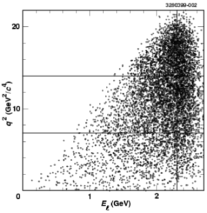
FIG. 2.: A simulated Dalitz plot, $q^{2}$ vs. $E_{\ell}$, for $B\to\rho\ell\nu$ decay. The lepton energy, $E_{\ell}$, is computed in the $\Upsilon(4S)\to B\bar{B}$ rest frame (lab frame), which differs slightly from the $B$ rest frame. This analysis is most sensitive to $B\to\rho\ell\nu$ events in the lepton-energy region to the right of the vertical line, $E_{\ell}>2.3$ GeV. The horizontal lines define the $q^{2}$ bins in the $\Delta\Gamma$ measurement: $0<q^{2}<7~{}{\rm GeV}^{2}/c^{4}$, $7<q^{2}<14~{}{\rm GeV}^{2}/c^{4}$, and $14<q^{2}<21~{}{\rm GeV}^{2}/c^{4}$. At high $q^{2}$, our lepton-energy requirement retains a much larger fraction of the phase space than it does at low $q^{2}$.

FIG. 3.: Theoretical $q^{2}$ distributions for the $B\rightarrow\rho\ell\nu$ form-factor models that we have considered: (a) over the full lepton-energy range and (b) for $E_{\ell}>2.3$ GeV. The lepton energy, $E_{\ell}$, is computed in the $\Upsilon(4S)\to B\bar{B}$ rest frame (lab frame), which differs slightly from the $B$ rest frame. In each plot, models have been normalized to equal areas. For high lepton energies, $E_{\ell}>2.3$ GeV, all of the models predict very similar $q^{2}$ distributions.

FF model	$\tilde{\Gamma}_{{\rm thy}}$ (ps-1)	$\Gamma(E_{\ell}>2.3~{}{\rm GeV})/\Gamma$ ($\%$)	$\Gamma(2.0<E_{\ell}<2.3~{}{\rm GeV})/\Gamma$ ($\%$)
ISGW2	14.2	$35$	$33$
LCSR	16.9	$24$	$28$
UKQCD	16.5	$27$	$30$
Wise/Ligeti+E791	19.4	$31$	$34$
Beyer/Melikhov	16.0	$27$	$30$

TABLE I.: $\tilde{\Gamma}_{{\rm thy}}$ and lepton-energy distribution predictions from each form-factor (FF) model. The lepton energy, $E_{\ell}$, is computed in the $\Upsilon(4S)\to B\bar{B}$ rest frame (lab frame), which differs slightly from the $B$ rest frame. For the branching fraction measurement, the primary source of model dependence is in the ratio $\Gamma(E_{\ell}>2.3~{}{\rm GeV})/\Gamma$. For the $|V_{ub}|$ measurement, there is significant additional model dependence arising from the quantity $\tilde{\Gamma}_{{\rm thy}}$.

Figure 3 shows the $q^{2}$ distribution predicted by our implementation of these models. Integrated over all lepton energies, there is a substantial difference among the models at low $q^{2}$ (large daughter-hadron recoil). At high lepton energy, however, the shapes of the $q^{2}$ distributions predicted by each of the form-factor models are very similar. To distinguish among form-factor models on the basis of the $q^{2}$ distribution, the lepton-energy region below 2.0 GeV must be probed.

Table II shows how the efficiency of the lepton-energy requirement varies with $q^{2}$ for each form-factor model. Our lepton-energy requirement retains a much larger fraction of the phase space at high $q^{2}$ than it does at low $q^{2}$. Thus, at high $q^{2}$, the efficiency is quite high and a small variation is seen among models. At low $q^{2}$, on the other hand, the efficiency is relatively low with a large variation among the form-factor models.

Integrating Eq. 21 over the angular variables, we obtain

$${{d\Gamma}\over{dq^{2}}}={{G_{F}^{2}}\over{96\pi^{3}}}|V_{q^{\prime}Q}|^{2}{{|{\bf p}_{V}|q^{2}}\over{m_{P}^{2}}}{\cal B}(V\rightarrow P_{1}P_{2})\times\biggl{[}|H_{+}(q^{2})|^{2}+|H_{-}(q^{2})|^{2}+|H_{0}(q^{2})|^{2}\biggr{]}.$$ (22)

Figure 4 shows the $d\Gamma/dq^{2}$ distribution for each term in Eq. 22. In each form-factor model, the term proportional to $|H_{-}|^{2}$ contributes the largest fraction of the total rate. As a consequence of the $V-A$ couplings of the $W$ boson the vector meson is more likely to have helicity $-1$ than $+1$. For $B\to\rho\ell\nu$ decay, this asymmetry is quite large, except at very high $q^{2}$ (low daughter-hadron recoil momentum) where the $A_{1}$ form factor dominates each of the helicity amplitudes and the $\rho$ is nearly unpolarized, and at small values of $q^{2}$, where only the zero-helicity component contributes significantly. Because the $|H_{+}|^{2}$ contribution is quite small, the theoretical error in the ${\cal B}(B\to\rho\ell\nu)$ and $\Delta\Gamma$ measurements is due primarily to the uncertainty in the relative size of $H_{-}(q^{2})$ and $H_{0}(q^{2})$.

Table III shows the predictions for $\Gamma/|V_{ub}|^{2}$ in bins of $q^{2}$ ($\Delta\tilde{\Gamma}_{{\rm thy}}$) for the form-factor models. These predictions can be used to extract $|V_{ub}|$ from a measurement of the $q^{2}$ distribution.

FIG. 4.: $d\Gamma/dq^{2}$ distributions for each of the three terms in Eq. 22: (a) the terms proportional to $|H_{-}|^{2}$ and $|H_{+}|^{2}$ and (b) the $|H_{0}|^{2}$ term.

FF model	$\Delta\Gamma(E_{\ell}>2.3~{}{\rm GeV})/\Delta\Gamma$	$\Delta\Gamma(E_{\ell}>2.3~{}{\rm GeV})/\Delta\Gamma$	$\Delta\Gamma(E_{\ell}>2.3~{}{\rm GeV})/\Delta\Gamma$
	($\%$)	($\%$)	($\%$)
	$0<q^{2}<7$ GeV${}^{2}/c^{4}$	$7<q^{2}<14$ GeV${}^{2}/c^{4}$	$14<q^{2}<21$ GeV${}^{2}/c^{4}$
ISGW2	$24$	$35$	$43$
LCSR	$12$	$25$	$38$
UKQCD	$15$	$28$	$39$
Wise/Ligeti+E791	$23$	$29$	$37$
Beyer/Melikhov	$14$	$27$	$38$

TABLE II.: The fraction of events predicted to have $E_{\ell}>2.3$ GeV in bins of $q^{2}$ for each form-factor (FF) model. The spread among these results is the largest component of the theoretical error in the $\Delta\Gamma$ measurement.

FF model	$\Delta\tilde{\Gamma}_{{\rm thy}}$ (ps-1)	$\Delta\tilde{\Gamma}_{{\rm thy}}$ (ps-1)	$\Delta\tilde{\Gamma}_{{\rm thy}}$ (ps-1)
	$0<q^{2}<7$ GeV${}^{2}/c^{4}$	$7<q^{2}<14$ GeV${}^{2}/c^{4}$	$14<q^{2}<21$ GeV${}^{2}/c^{4}$
ISGW2	2.8	6.1	5.3
LCSR	5.4	6.6	4.9
UKQCD	4.5	6.7	5.3
Wise/Ligeti+E791	3.5	8.4	7.5
Beyer/Melikhov	4.3	6.4	5.3

TABLE III.: Partial rate ($\Delta\tilde{\Gamma}_{{\rm thy}}$) predictions in $q^{2}$ bins from each form-factor (FF) model.

III Data sample and event selection

The data used in this analysis were collected using the CLEO II detector [27] located at the Cornell Electron Storage Ring (CESR), operating near the $\Upsilon(4S)$ resonance. We have analysed a $3.1$ fb^-1 sample taken on the resonance, corresponding to approximately $3.3\times 10^{6}$ $B\bar{B}$ pairs. Additionally, we examine a $1.7$ fb^-1 sample taken at a center-of-mass energy $60$ MeV below the $\Upsilon(4S)$ mass. These off-resonance data, which have an energy below the threshold for $B\bar{B}$ production, are used to measure the continuum background.

The CLEO II detector is designed to provide excellent charged- and neutral-particle reconstruction efficiency and resolution. Three cylindrical tracking chambers are surrounded by a time-of-flight (TOF) system, a CsI calorimeter, and a muon tracking system. The nearly complete solid-angle coverage of both the tracking system and calorimeter is exploited in this analysis to obtain information on the momentum of the neutrino.

To be considered as a hadron or lepton candidate, charged tracks must satisfy several requirements. The impact parameter of the track along and transverse to the beam direction must be less than 5 cm and 2 mm, respectively. The spread in the impact parameter along the beam direction is dominated by the beam width in that direction and is approximately 1.5 cm. Transverse to the beam direction, the resolution on the impact parameter is approximately $0.3$ mm. The r.m.s. residual for the hits on the track must be less than 1 mm. Finally, we require that at least 15 out of the 67 tracking layers be used in the track fit.

Electron and muon identification requirements are chosen to achieve high efficiency and a low hadronic fake rate. We require $|\cos\theta|<0.85$, where $\theta$ is the polar angle of the track’s momentum vector with respect to the beam axis. Electrons are identified primarily using the ratio of the calorimeter energy to track momentum ($E/p$) and specific ionization ($dE/dx$) information. Muon candidates are found by extrapolating tracks from the central detector into the muon counters; such candidates are required to penetrate at least seven interaction lengths of iron. For electrons (muons) that satisfy the tracking requirements described above as well as the lepton-energy requirements of our analysis, the efficiency of these lepton-identification requirements is approximately $94\%$ ($82\%$). The fraction of hadrons passing electron (muon) identification criteria is determined from data and is approximately $0.1\%~{}(0.6\%)$.

Photon candidates are associated with CsI calorimeter clusters that are not matched to any charged track. Individual photons are required to have energy, $E_{\gamma}$, greater than 30 MeV. To be considered in a $\pi^{0}$ candidate, two photons must have a combined invariant mass, $M_{\gamma\gamma}$, within $2\sigma$ of the nominal $\pi^{0}$ mass. Their combined energy, $E_{\gamma\gamma}$, is required to be greater than 325 MeV. In addition, we require that at least one photon satisfy $|\cos\theta_{\gamma}|<0.71$, where $\theta_{\gamma}$ is the polar angle with respect to the beam axis. Each photon candidate is included in at most one $\pi^{0}$ candidate.

To search for $B\rightarrow\rho\ell\nu$, $B\rightarrow\omega\ell\nu$, and $B\rightarrow\pi\ell\nu$ events, electron or muon candidates are combined with $\pi^{\pm}\pi^{0}$, $\pi^{+}\pi^{-}$, $\pi^{+}\pi^{-}\pi^{0}$, $\pi^{\pm}$, or $\pi^{0}$ candidates. Combinatoric backgrounds are suppressed by requiring candidates for these hadronic systems to have a momentum greater than 300 MeV/$c$; these backgrounds are further suppressed in the $\pi^{+}\pi^{-}\pi^{0}$ mode by making a cut on the $\omega\to\pi^{+}\pi^{-}\pi^{0}$ Dalitz amplitude. We require that the $\pi^{+}$, $\pi^{-}$, and $\pi^{0}$ be configured such that the decay probability density ($d\Gamma\propto|{\bf p}_{\pi^{+}}\times{\bf p}_{\pi^{-}}|^{2}$ where ${\bf p}_{\pi^{+}}$ and ${\bf p}_{\pi^{-}}$ are evaluated in the $\omega$ rest frame) is at least $12\%$ of its maximum value.

We define the missing momentum in the event to be

$${\bf p}_{{\rm miss}}\equiv-\Sigma{\bf p}_{i},$$ (23)

where the sum is over reconstructed charged tracks and photon candidates in the event. If the event contains no undetected particles other than the $\nu$ from the $B\to\rho\ell\nu$ decay, ${\bf p}_{{\rm miss}}\approx{\bf p}_{{\nu}}$. The resolution on ${\bf p}_{{\rm miss}}$ is determined by undetected particles, such as $K^{0}_{L}$ mesons, and our experimental resolution. As discussed in the following section, ${\bf p}_{{\rm miss}}$ is used to calculate one of our three fit variables.

Background events come from continuum, $b\rightarrow c\ell\nu$, $b\rightarrow u\ell\nu$ (other than $B\to\rho\ell\nu$ or $B\to\omega\ell\nu$), and events with hadrons misidentified as leptons. The $b\rightarrow c\ell\nu$ background is dominant at lower lepton energy. To distinguish signal events from background most effectively, we consider three lepton-energy ranges:

• $E_{\ell}>2.3$ GeV (denoted as HILEP in the remainder of this paper),

• $2.0<E_{\ell}<2.3$ GeV (LOLEP),

• $1.7<E_{\ell}<2.0$ GeV,

where the lepton energy, $E_{\ell}$, is computed in the $\Upsilon(4S)\to B\bar{B}$ rest frame (lab frame). The $B$-meson rest frame is moving with a small velocity, $\beta\approx 0.065$, relative to the $\Upsilon(4S)$ frame. Sensitivity to $B\rightarrow\rho\ell\nu$ decay is best in the HILEP lepton-energy bin where the $b\rightarrow c\ell\nu$ background is quite small. Here, the backgrounds are primarily continuum and $b\rightarrow u\ell\nu$ events. In LOLEP, the $b\rightarrow c\ell\nu$ background dominates, but the $b\rightarrow u\ell\nu$ contributions in this region are not negligible. Events with $1.7<E_{\ell}<2.0$ GeV are completely dominated by $b\to c\ell\nu$ decays and are included primarily to verify our understanding of this source of background.

Because our best sensitivity to $B\to\rho\ell\nu$ is in the HILEP region, suppression of continuum background is a key issue in the analysis. At the $\Upsilon(4S)$ center-of-mass energy, $\Upsilon(4S)\to B\bar{B}$ decays can be distinguished from continuum events, which have a three times larger cross section, on the basis of various quantities that describe the overall distribution of tracks and photons in the event. Such event shape, or event topology, variables exploit the fact that the $B$ mesons are produced nearly at rest so their decay products are distributed roughly uniformly in solid angle. In contrast, continuum events yield a much more collimated or jet-like event topology. We use several event-shape requirements in selecting our sample:

• The ratio of the second to zeroth Fox-Wolfram moments [28] is required to be less than $0.3$. This ratio of moments tends to be close to zero for spherical events and up to unity for jet-like events.

• $\rho\ell$, $\omega\ell$, and $\pi\ell$ candidates are required to have $|\cos\theta_{{\rm thrust}}|\leq 0.8$, where $\theta_{{\rm thrust}}$ is defined to be the angle between the thrust axis of the candidate system and the thrust axis of the rest of the event.

• We select events with $|\cos\theta_{{\rm miss}}|\leq 0.9$, where $\theta_{{\rm miss}}$ is the polar angle of the missing momentum (${\bf p}_{{\rm miss}}$) with respect to the beam axis (see Eq. 23).

• We select events whose energy is evenly distributed around the momentum axis of the candidate lepton using a Fisher discriminant [29]. The input variables to the Fisher discriminant are the track and CsI cluster energies in nine cones of equal solid angle around the lepton-momentum axis. Energy in $B\bar{B}$ events tends to be more evenly distributed in these cones than in jet-like continuum events.

To suppress combinatoric backgrounds from $b\rightarrow c\ell\nu$ and from $b\rightarrow u\ell\nu$ sources other than $B\rightarrow\rho\ell\nu$ and $B\to\omega\ell\nu$, we require that the event kinematics be consistent with these signal modes. Using the constraints $E_{{B}}=E_{{\rm Beam}}$ and $p_{\nu}^{2}=0=(p_{B}-p_{\rho}-p_{\ell})^{2}$, we compute the angle between the $B$ momentum direction and that of the reconstructed ${Y}\equiv(\rho,~{}\omega,~{}\pi)+\ell$ system:

$$\cos\theta_{{BY}}\equiv{{2E_{B}E_{Y}-m_{B}^{2}-m_{Y}^{2}}\over{2|{\bf p}_{B}||{\bf p}_{Y}|}}.$$ (24)

The distribution of $|{\bf p}_{B}|\cdot\cos\theta_{BY}$ is shown in Fig. 5a for signal, continuum, and $b\to c\ell\nu$ events that satisfy all other analysis requirements. We require that $|{\bf p}_{B}|\cdot|\cos\theta_{BY}|\leq 385$ MeV/$c$. For well-reconstructed signal events with a $B$ momentum of less than 385 MeV/$c$, this cut is $100\%$ efficient, but $b\rightarrow u\ell\nu$ (non-signal modes), $b\rightarrow c\ell\nu$, and continuum events often produce unphysical values of $\cos\theta_{{BY}}$ and can be rejected. At CESR, the average $B$ meson momentum is approximately 320 MeV/$c$, with a standard deviation of 50 MeV/$c$ due to the beam energy spread from the emission of synchrotron radiation, so this cut is nearly $100\%$ efficient for well-reconstructed signal events.

FIG. 5.: Signal and background distributions for the HILEP $\pi\pi$ modes: (a) $|{\bf p}_{B}|\cos\theta_{{\rm BY}}$ for events that pass all other requirements including $|M(\pi\pi)-M(\rho)|<0.15~{}{\rm GeV}/c^{2}$ and $|\Delta E|<0.5~{}{\rm GeV}$ and (b) $M(\pi\pi)$ for events that pass all requirements including $|\Delta E|<0.5~{}{\rm GeV}$. Shown are the Monte Carlo signal, continuum data, and Monte Carlo $b\to c\ell\nu$ contributions. Each has been normalized using the results of the likelihood fit described in Sec. IV. The signal contribution includes events from one signal mode that have been reconstructed in another signal mode. The $|{\bf p}_{B}|\cdot|\cos\theta_{BY}|\leq 385$ MeV/$c$ requirement keeps almost all signal events, while rejecting much of the background.

Finally, we compare the direction of the missing momentum (${\bf p}_{{\rm miss}}$) with that of the neutrino momentum (${\bf p}_{\nu}$) inferred from the ${\bf p}_{\nu}={\bf p}_{B}-{\bf p}_{Y}$ momentum. The latter is known to within an azimuthal ambiguity about the ${\bf p}_{Y}$ direction because the magnitude, but not the direction, of the $B$ meson momentum is known. We require that the minimum difference in the angle between these two directions be less than 0.6 radians.

Because the $\rho$ has a large width and we are reconstructing several different hadronic modes, events with multiple entries passing all of the above requirements are common. To avoid the statistical difficulties associated with this, we choose one combination per event after all other criteria are imposed, picking the combination with $|{\bf p}_{Y}+{\bf p}_{{\rm miss}}|$ closest to $|{\bf p}_{B}|$.

The large $\rho$ width also leads to an important effect in signal events. The candidate $\pi\pi$ system may not consist of the true daughter particles of the $\rho$. For example, it is possible for a $B\to\rho^{0}\ell\nu$ event to satisfy the analysis requirements for the $B\to\rho^{+}\ell\nu$ channel. In addition, $B\to\omega\ell\nu$ events can feed into the $B\to\rho\ell\nu$ channels. We denote this contribution as crossfeed signal. Although the kinematic distributions of these events are somewhat different from correctly reconstructed signal events, the crossfeed contribution is produced by signal processes, and it is counted as such.

Figure 5b shows the $M(\pi\pi)$ distribution expected from signal, continuum, and $b\to c\ell\nu$ events in the HILEP $\pi\pi$ modes. Each contribution has been normalized using the results of the likelihood fit described in Sec. IV.

IV Fit method

We perform a binned maximum-likelihood fit using MINUIT [30] in three lepton-energy ranges and five decay modes. In addition to lepton energy, we fit two kinematic variables, so we are in effect performing a three dimensional correlated fit. Our fit includes contributions from $B\rightarrow\rho\ell\nu$, $B\to\omega\ell\nu$, $B\rightarrow\pi\ell\nu$, other $b\rightarrow u\ell\nu$ modes, $b\rightarrow c\ell\nu$, continuum events, as well as a contribution from hadrons faking leptons. In this section, we describe the fit variables and constraints, the modeling of signal and background components, and our method for extracting the rate as a function of $q^{2}$.

The three fit variables, $E_{\ell}$, $M_{\rm had}$, and $\Delta E$, are constructed from the three decay products in semileptonic decay: the lepton, the final-state hadron, and the neutrino. The three lepton-energy bins were discussed in Sec. III. The invariant mass of the daughter hadron, $M_{\rm had}$, is reconstructed in the $\pi^{+}\pi^{-}$ and $\pi^{\pm}\pi^{0}$ channels for $B\to\rho\ell\nu$ and in the $\pi^{+}\pi^{-}\pi^{0}$ channel for $B\to\omega\ell\nu$. The bin size for the fit is $90$ MeV/$c^{2}$ for both $M(\pi\pi)$ and $M(\pi\pi\pi)$. The momentum of the hadron is not used as a fit variable but is the basis for measuring the $q^{2}$ distribution after the fit is performed.

The presence of a neutrino consistent with $B\to\rho\ell\nu$ decay is signaled by a peak in the distribution of

$$\Delta E\equiv E_{\rho}+E_{\ell}+|{\bf p}_{{\rm miss}}|-E_{{\rm Beam}}$$ (25)

at $\Delta E=0$. Backgrounds from $b\rightarrow c\ell\nu$ and $b\rightarrow u\ell\nu$ (except for $B\to\pi\ell\nu$) events tend to have $\Delta E<0$. On the other hand, $B\rightarrow\pi\ell\nu$ events have $\Delta E>0$ when reconstructed in the $\pi\pi$ or $\pi^{+}\pi^{-}\pi^{0}$ modes, since extra particles beyond the actual $B$ decay products are included in the decay hypothesis. The $\Delta E$ bin size for the fit is 200 MeV.

$\Delta E$ vs. $M(\pi\pi)$ distributions for signal and background contributions in the HILEP region are shown in Fig. 6. Shapes of distributions for signal, $b\to c\ell\nu$, and $b\to u\ell\nu$ are taken from Monte Carlo simulations using theoretical models of $B$-meson decays and full detector simulations based on GEANT [31], while the continuum background is measured with the off-resonance data. An additional background, not shown, arises from hadrons passing the lepton identification requirements in $B\bar{B}$ events. This contribution is determined using measured fake rates and data, as described below. The data or Monte Carlo samples that are used to estimate the non-continuum contributions are sufficiently large that their statistical fluctuations are negligible compared with those of the data. We now discuss each of these fit components in more detail.

FIG. 6.: Signal and background $\Delta E$ vs. $M(\pi\pi)$ distributions for the combined $\pi^{\pm}\pi^{0}$ and $\pi^{+}\pi^{-}$ modes in HILEP: (a) the direct signal contribution; background events from (b) the continuum; (c) $b\to c\ell\nu$ events; (d) $b\to u\ell\nu$ events. The continuum contribution is modeled using the off-resonance data, while the other contributions are taken from Monte Carlo samples. Signal events are centered on $\Delta E=0$ and are clustered around the $\rho$ mass in $M(\pi\pi)$.

For signal, the Monte Carlo sample provides the shapes of the three-dimensional distribution of $E_{\ell}$, $M_{{\rm had}}$, and $\Delta E$. There is very little model dependence in the $\Delta E$ vs. $M_{{\rm had}}$ distributions, but the distribution of signal events across the three lepton-energy bins varies significantly among form-factor models. The variation among the $B\rightarrow\rho\ell\nu$ form-factor models is a significant systematic error for our measurement of ${\cal B}(B\rightarrow\rho\ell\nu)$ and $|V_{ub}|$.

There are a large number of crossfeed signal events, as described in the previous section. The size of the crossfeed contribution relative to the direct signal is determined using Monte Carlo simulation. These events are misreconstructed signal decays and their kinematic distributions can be somewhat different from direct signal events.

Isospin and quark-model relations are used to constrain the relative normalizations of $B^{0}\rightarrow\rho^{-}\ell^{+}\nu$, $B^{+}\rightarrow\rho^{0}\ell^{+}\nu$, and $B^{+}\rightarrow\omega\ell^{+}\nu$ and, separately, those of $B^{0}\rightarrow\pi^{-}\ell^{+}\nu$ and $B^{+}\rightarrow\pi^{0}\ell^{+}\nu$. Isospin symmetry implies that

$$\Gamma(B^{0}\rightarrow\rho^{-}\ell^{+}\nu) = 2\Gamma(B^{+}\rightarrow\rho^{0}\ell^{+}\nu),$$ (26)

$$\Gamma(B^{0}\rightarrow\pi^{-}\ell^{+}\nu) = 2\Gamma(B^{+}\rightarrow\pi^{0}\ell^{+}\nu),$$ (27)

while the $\omega$ and $\rho^{0}$ wave functions are expected to be very similar in the quark model, giving

$$\Gamma(B^{+}\rightarrow\rho^{0}\ell^{+}\nu)=\Gamma(B^{+}\rightarrow\omega\ell^{+}\nu).$$ (28)

Possible isospin breaking effects are discussed in Refs. [32, 33]. We assume that the $\Upsilon(4S)$ decays only to $B\bar{B}$ in equal proportions of $B^{0}\bar{B}^{0}$ and $B^{+}B^{-}$ mesons ($f_{+-}/f_{00}=1.0\pm 0.1$). We also use the value $\tau_{B^{+}}/\tau_{B^{0}}=1.04\pm 0.04$ [34] for the ratio of charged to neutral $B$-meson lifetimes.

The shape and normalization of the continuum background are measured using the off-resonance data sample. The statistical fluctuations in the off-resonance sample are accounted for by fitting the on- and off-resonance samples simultaneously, accounting for the difference in luminosity and cross section. For each bin in the fit, the mean number of continuum background events is determined so as to maximize the combined likelihood.

The normalization of the $b\to c\ell\nu$ background is determined to a large extent from the data. This background arises primarily from two extensively studied decays, $B\to D\ell\nu$ and $B\to D^{*}\ell\nu$, and the associated kinematic distributions are well known. As for the signal modes, the shapes of the $\Delta E$ vs. $M_{{\rm had}}$ distributions due to $b\to c\ell\nu$ are obtained using the Monte Carlo calculations. With these constraints, there remain 15 $b\to c\ell\nu$ normalization parameters, one for each of the five signal modes in each of three lepton-energy bins.

In our fit, there are in fact only seven free parameters associated with the $b\to c\ell\nu$ background, defined in the following way. Five of the parameters, one for each signal mode, are scale factors that give the overall normalization of the $b\to c\ell\nu$ background relative to that expected from the Monte Carlo simulation. Two additional parameters describe the ratios of scale factors among the three lepton-energy bins. A common set of ratios is used for all five modes, so we have two rather than $2\times 5$ parameters for the $b\to c\ell\nu$ lepton energy spectrum. The reason for this choice is that the same set of background modes, dominated by $B\to D^{*}\ell\nu$ and $B\to D\ell\nu$, contributes to each of the five signal modes. The relative contributions of the different $b\to c\ell\nu$ modes are essentially independent of the $b\to u\ell\nu$ mode we reconstruct. In Sec. V, we show that our fit results for all seven of these $b\to c\ell\nu$ background parameters agree well with Monte Carlo predictions.

The normalization for the contribution from $B\to\pi\ell\nu$ decay is also determined by the data. As for the $B\to\rho\ell\nu$ contribution, form-factor models are used to describe the kinematic distributions. A systematic error is assigned based on the variation observed in the $B\to\rho\ell\nu$ fit results for different $B\to\pi\ell\nu$ form-factor models.

The ISGW2 [9] predictions are used to model the distributions of $b\rightarrow u\ell\nu$ sources other than $B\to\rho\ell\nu$, $B\to\omega\ell\nu$, and $B\to\pi\ell\nu$ for resonances up to the $\rho(1450)$. The dominant resonances are $\eta$, $b_{1}$, and $a_{1}$. The uncertainty on the composition of this background is considered as a systematic error. To reduce this systematic uncertainty, we allow for a separate normalization for the $b\to u\ell\nu$ component in each lepton-energy bin.

The small contribution from fake leptons is found using the data. The shapes of the $\Delta E$ vs. $M(\pi\pi)$ distribution, along with that of $E_{\ell}$, are found by combining $\rho$ candidates with charged tracks not identified as leptons. These combinations are required to pass all analysis criteria except for the lepton-identification requirements. The normalization of the fake-lepton component is determined by measurements of the probability for hadrons to satisfy the lepton identification requirements using $\pi$, $K$, and $p$ samples from the data (see Sec. III).

There are thus twelve free parameters in the fit:

• ${\cal B}(B\rightarrow\rho\ell\nu)$ (1 parameter).

• ${\cal B}(B\rightarrow\pi\ell\nu)$ (1 parameter).

• The yield of $b\rightarrow u\ell\nu$ events in each lepton-energy bin (3 parameters).

• The seven parameters that describe the normalization of the $b\rightarrow c\ell\nu$ contribution.

We do not include a contribution from $B\to\pi\pi\ell\nu$ nonresonant events in our fit. Instead, we use the data to constrain the size of this contribution and assign a systematic error (see Sec. VI).

The ${\cal B}(B\rightarrow\rho\ell\nu)$ result from the likelihood fit is used to compute

$$|V_{ub}|=\sqrt{{{\cal B}\over{\tilde{\Gamma}_{{\rm thy}}\tau_{B^{0}}}}}.$$ (29)

${\cal B}$ is the result for the $B^{0}\to\rho^{-}\ell^{+}\nu$ branching fraction from the likelihood fit, which depends on the form-factor model used to describe the signal distributions. Results for $\tilde{\Gamma}_{{\rm thy}}$ are given for each of the five form-factor models in Table I. We use $\tau_{B^{0}}=1.56\pm 0.04$ ps [34].

The likelihood fit results are also used to measure the $q^{2}$ distribution in $B\to\rho\ell\nu$ decay. The large $b\to c\ell\nu$ backgrounds in LOLEP limit this measurement to the HILEP lepton-energy region. To determine the $q^{2}$ distribution, we consider events in the $\pi^{\pm}\pi^{0}$ and $\pi^{+}\pi^{-}$ modes with  $|M(\pi\pi)-M(\rho)|<0.15$ GeV/$c^{2}$ and $|\Delta E|<0.5$ GeV. The background contributions in each $q^{2}$ interval are estimated using the results of the likelihood fit. We count the number of events in the background samples and subtract them from the data. Below we discuss the determination of $q^{2}$ for each event and describe the extraction of the $q^{2}$ distribution.

If the $B$ meson momentum vector were known, $q^{2}$ could be determined unambiguously from the energy of the daughter hadron. For $B\to\rho\ell\nu$,

$$q^{2}=M_{B}^{2}+M_{\rho}^{2}-2E_{B}E_{\rho}+2{\bf p}_{B}\cdot{\bf p}_{\rho}.$$ (30)

We know the magnitude of the $B$ momentum, but not its direction, which introduces an uncertainty in $q^{2}$. Using the beam-energy constraint, we compute the minimum and maximum allowed $q^{2}$ values for each $\rho+\ell$ combination. These correspond to the kinematic configurations where the $B$ momentum direction is closest to, or furthest from, the $\rho$ momentum direction. The midpoint of the allowed $q^{2}$ range is our estimate of $q^{2}$. The $q^{2}$ resolution function is shown in Fig. 7.

To find the true $q^{2}$ distribution from the data, we must determine the efficiency of our analysis requirements as a function of $q^{2}$, including the smearing effects shown in Fig. 7. We perform this measurement in three equal bins of $q^{2}$. Monte Carlo simulation is used to compute the efficiency of events generated with a particular $q^{2}$ to be reconstructed at a different value of $q^{2}$. This efficiency matrix is computed for each of the five form-factor models that we consider; model dependence arises primarily from the efficiency of the $E_{\ell}>2.3$ GeV requirement. The reconstructed $q^{2}$ distribution of the HILEP data and this efficiency matrix are used to determine the true $q^{2}$ distribution.

FIG. 7.: The $q^{2}$ resolution for signal Monte Carlo events. The curve shows a fit to the Monte Carlo events (shaded histogram) using two Gaussians. The narrow ($\sigma=0.4$ GeV${}^{2}/c^{4}$) component is due to events where the correct hadronic mode is reconstructed. The broader ($\sigma=2.6$ GeV${}^{2}/c^{4}$) component is from crossfeed events. We account for this smearing in our measurement of $\Delta\Gamma$ in bins of $q^{2}$. The full $q^{2}$ range for $B\to\rho\ell\nu$ is $\Delta q^{2}\approx 21$ GeV${}^{2}/c^{4}$.

V Fit results

The signal and background yields extracted from the fit in HILEP and LOLEP are shown in Tables IV and V for the $\pi\pi$ and $\pi^{+}\pi^{-}\pi^{0}$ modes. The signal yields for the combined $\pi^{+}\pi^{0}$ and $\pi^{+}\pi^{-}$ modes in HILEP, where our sensitivity to the signal is best, are $123\pm 18$ (direct) and $93\pm 14$ (crossfeed), for a total of $216\pm 32$ signal events. The five $b\rightarrow c\ell\nu$ normalization scale factors are consistent with Monte Carlo predictions to better than $5\%$. The two scale factor ratios that determine the lepton-energy distribution for the $b\to c\ell\nu$ contribution are within one standard deviation of unity. The $b\rightarrow u\ell\nu$ (modes other than $B\to\rho\ell\nu$, $B\to\omega\ell\nu$, and $B\to\pi\ell\nu$) normalizations in the three lepton-energy bins agree with each other to better than $20\%$, within one standard deviation, indicating that the ISGW2 cocktail of $b\rightarrow u\ell\nu$ modes is adequate, at least to within our sensitivity.

	$\rho^{\pm}$ HI	$\rho^{0}$ HI	$\omega$ HI	$\rho^{\pm}$ LO	$\rho^{0}$ LO	$\omega$ LO
$\Upsilon({\rm 4S})$ yield	198	621	460	2249	7298	8552
$e^{+}e^{-}\rightarrow q\bar{q}$ bkg.	$63\pm 11$	$248\pm 22$	$250\pm 22$	$127\pm 16$	$398\pm 28$	$437\pm 29$
$b\rightarrow c\ell\nu$ bkg.	$39\pm 5$	$90\pm 7$	$52\pm 5$	$1941\pm 47$	$6419\pm 114$	$7804\pm 129$
fake lepton bkg.	$4\pm 2$	$13\pm 7$	$10\pm 5$	$11\pm 7$	$35\pm 21$	$44\pm 22$
$b\rightarrow u\ell\nu$ bkg.	$25\pm 10$	$57\pm 23$	$43\pm 17$	$97\pm 24$	$222\pm 57$	$236\pm 60$
$B\rightarrow\pi\ell\nu$ bkg.	$9\pm 3$	$20\pm 6$	$4\pm 1$	$15\pm 5$	$32\pm 10$	$6\pm 2$
Direct sig.	$56\pm 8$	$67\pm 10$	$21\pm 3$	$61\pm 9$	$79\pm 12$	$31\pm 5$
Xfeed sig.	$13\pm 2$	$80\pm 12$	$32\pm 5$	$23\pm 3$	$100\pm 15$	$52\pm 8$

TABLE IV.: Summary of data yields for the $\rho^{\pm}$, $\rho^{0}$, and $\omega$ modes with lepton energies between 2.3 and 2.7 GeV (HILEP) and between 2.0 and 2.3 GeV (LOLEP). Yields of the background contributions are insensitive to the form-factor model used to model $B\rightarrow\rho\ell\nu$ events; the yields presented in this table were obtained using the UKQCD model. The $b\rightarrow u\ell\nu$ background includes all $B\rightarrow X_{u}\ell\nu$ modes except for $\rho$, $\omega$, and $\pi$. The crossfeed (Xfeed) signal contribution corresponds to events from one vector mode passing the selection cuts of another vector mode ($\rho^{0}\ell\nu\leftrightarrow\rho^{\pm}\ell\nu$ or $\rho\ell\nu\leftrightarrow\omega\ell\nu$) and is constrained to the signal in the fit. All errors are statistical only. The errors on the direct and crossfeed signal yields are completely correlated, as are those on the yields of $B\rightarrow\pi\ell\nu$ events. Errors on the $b\rightarrow u\ell\nu$ background are completely correlated among modes, but not between HILEP and LOLEP.

	$\rho^{\pm}$ HI	$\rho^{0}$ HI	$\omega$ HI	$\rho^{\pm}$ LO	$\rho^{0}$ LO	$\omega$ LO
Signal eff. (ISGW2)	0.040	0.091	0.032	0.039	0.094	0.040
Signal yield (ISGW2)	$58\pm 9$	$68\pm 10$	$21\pm 3$	$55\pm 9$	$70\pm 11$	$26\pm 4$
Xfeed yield (ISGW2)	$14\pm 2$	$80\pm 12$	$34\pm 5$	$20\pm 3$	$89\pm 13$	$48\pm 7$
Signal eff. (LCSR)	0.026	0.061	0.022	0.030	0.076	0.034
Signal yield (LCSR)	$56\pm 8$	$66\pm 10$	$21\pm 3$	$64\pm 10$	$84\pm 13$	$33\pm 5$
Xfeed yield (LCSR)	$14\pm 2$	$80\pm 11$	$32\pm 5$	$24\pm 3$	$105\pm 15$	$54\pm 8$
Signal eff. (UKQCD)	0.031	0.070	0.025	0.033	0.083	0.036
Signal yield (UKQCD)	$56\pm 8$	$67\pm 10$	$21\pm 3$	$61\pm 9$	$79\pm 12$	$31\pm 5$
Xfeed yield (UKQCD)	$14\pm 2$	$80\pm 12$	$33\pm 5$	$23\pm 3$	$100\pm 15$	$52\pm 8$
Signal eff. (Wise/Ligeti+E791)	0.035	0.080	0.028	0.037	0.094	0.040
Signal yield (Wise/Ligeti+E791)	$56\pm 8$	$66\pm 10$	$21\pm 3$	$60\pm 9$	$79\pm 12$	$30\pm 4$
Xfeed yield (Wise/Ligeti+E791)	$14\pm 2$	$80\pm 12$	$32\pm 5$	$24\pm 3$	$102\pm 15$	$52\pm 8$
Signal eff. (Beyer/Melikhov)	0.029	0.067	0.024	0.033	0.083	0.036
Signal yield (Beyer/Melikhov)	$55\pm 8$	$66\pm 10$	$21\pm 3$	$61\pm 10$	$81\pm 12$	$31\pm 5$
Xfeed yield (Beyer/Melikhov)	$14\pm 2$	$80\pm 12$	$32\pm 5$	$24\pm 3$	$104\pm 15$	$53\pm 8$

TABLE V.: Summary of direct and crossfeed (Xfeed) signal yields for the $\rho^{\pm}$, $\rho^{0}$, and $\omega$ modes with lepton energies between 2.3 and 2.7 GeV (HILEP) and between 2.0 and 2.3 GeV (LOLEP). Signal efficiencies are normalized to the number of events in the full lepton-energy range. The crossfeed contribution corresponds to events from one vector mode passing the selection cuts of another vector mode ($\rho^{0}\ell\nu\leftrightarrow\rho^{\pm}\ell\nu$ or $\rho\ell\nu\leftrightarrow\omega\ell\nu$) and is constrained to the signal in the fit. All errors are statistical only. Errors on the direct and crossfeed signal yields are completely correlated.

We show projections of the fit in both signal- and background-dominated regions of the $\Delta E$ vs. $M(\pi\pi)$ distributions. Figure 8 shows HILEP and LOLEP projections onto $M(\pi\pi)$ for $|\Delta E|<0.5$ GeV and onto $\Delta E$ for $|M(\pi\pi)-M(\rho)|<0.15$ GeV/$c^{2}$. We observe a significant $B\to\rho\ell\nu$ signal in the $M(\pi\pi)$ and $\Delta E$ distributions in HILEP. Figure 9 shows the same distributions for sidebands with $|\Delta E|>0.5$ GeV and $|M(\pi\pi)-M(\rho)|>0.15$ GeV/$c^{2}$, where we expect much less signal. In both signal- and background-dominated distributions, we observe good agreement between the data and the fit projections. In the projections shown, the signal component is modeled using the ISGW2 form-factor model, and the continuum contribution has been subtracted.

FIG. 8.: Projections of the fit for the combined $\rho^{\pm}$ and $\rho^{0}$ modes for HILEP ($E_{\ell}>2.3$ GeV, upper plots) and LOLEP ($2.0<E_{\ell}<2.3$ GeV, lower plots): (a) $M(\pi\pi)$ for HILEP after a $|\Delta E|<0.5$ GeV cut; (b) $\Delta E$ for HILEP after a $|M(\pi\pi)-M({\rho})|<0.15$ GeV/$c^{2}$ cut; (c) $M(\pi\pi)$ for LOLEP after a $|\Delta E|<0.5$ GeV cut; (d) $\Delta E$ for LOLEP after a $|M(\pi\pi)-M({\rho})|<0.15$ GeV/$c^{2}$ cut. In each plot, the points with error bars show the on-resonance data after continuum-background subtraction, while the histogram shows the projection of the fit. The contributions to the fit are the direct and crossfeed components of the signal (unshaded regions, above and below the dashed line, respectively); the background from $b\to u\ell\nu$ non-signal modes (darkly-shaded region); and the background from $b\to c\ell\nu$ (lightly-shaded region). The $b\to u\ell\nu$ background includes $B\to\pi\ell\nu$ contributions.

FIG. 9.: Projections of the fit for the combined $\rho^{\pm}$ and $\rho^{0}$ modes for HILEP ($E_{\ell}>2.3$ GeV, upper plots) and LOLEP ($2.0<E_{\ell}<2.3$ GeV, lower plots): (a) $M(\pi\pi)$ for HILEP after a $|\Delta E|>0.5$ GeV cut; (b) $\Delta E$ for HILEP after a $|M(\pi\pi)-M({\rho})|>0.15$ GeV/$c^{2}$ cut; (c) $M(\pi\pi)$ for LOLEP after a $|\Delta E|>0.5$ GeV cut; (d) $\Delta E$ for LOLEP after a $|M(\pi\pi)-M({\rho})|>0.15$ GeV/$c^{2}$ cut. In each plot, the points with error bars show the on-resonance data after continuum-background subtraction, while the histogram shows the projection of the fit. The contributions to the fit are the direct and crossfeed components of the signal (unshaded regions, above and below the dashed line, respectively); the background from $b\to u\ell\nu$ non-signal modes (darkly-shaded region); and the background from $b\to c\ell\nu$ (lightly-shaded region). The $b\to u\ell\nu$ background includes $B\to\pi\ell\nu$ contributions.

The $b\rightarrow c\ell\nu$ background is quite small in the HILEP plots but is dominant in all of the LOLEP projections. The peak in the LOLEP $\pi\pi$ modes at large $M(\pi\pi)$ is due to $B\rightarrow D\ell\nu$, with $D\rightarrow K\pi$, where the $K$ has been misinterpreted as a pion. LOLEP projections in Fig. 9 show that the shape of the $b\to c\ell\nu$ Monte Carlo distribution describes the data well in regions of the fit where the $b\to u\ell\nu$ contributions are small. In Fig. 8, the shape of the $M(\pi\pi)$ distribution in the LOLEP lepton-energy bin indicates that the $b\rightarrow u\ell\nu$ contributions are necessary to describe properly the data below the $b\rightarrow c\ell\nu$ lepton-energy endpoint region. We do not show fit projections for the data with $E_{\ell}<2.0$ GeV, but the fit agrees well with the data in this region. The $b\to c\ell\nu$ Monte Carlo simulates $M(\pi\pi)$ and $\Delta E$ projections of the data well in both shape and normalization.

Figure 10 shows the reconstructed $q^{2}$ and lepton-energy distributions for the $\pi\pi$ modes with $|\Delta E|<0.5$ GeV and $|M(\pi\pi)-M(\rho)|<0.15$ GeV/$c^{2}$ requirements. We observe good agreement between the data and the $q^{2}$ distribution predicted in HILEP by the form-factor models. The lepton-energy spectrum predicted from the fit results shows good agreement with the data over the full range of lepton-energy used ($E_{\ell}>1.7$ GeV). A large excess in the lepton-energy spectrum, consistent with the fit projection, is observed above the continuum contribution in the region beyond the $b\to c\ell\nu$ lepton energy endpoint.

FIG. 10.: Projections of the kinematic variables: (a) $q^{2}$ and (b) $E_{\ell}$. Both distributions are shown for the combined $\rho^{\pm}$ and $\rho^{0}$ modes for events with $|\Delta E|<0.5$ GeV and $|M(\pi\pi)-M({\rho})|<0.15$ GeV/$c^{2}$. The $q^{2}$ distribution is shown only for events with $E_{\ell}>2.3$ GeV. In each plot, the points with error bars show the on-resonance data after continuum-background subtraction, while the histogram shows the projection of the fit. The contributions to the fit are the direct and crossfeed components of the signal (unshaded regions, above and below the dashed line, respectively); the background from $b\to u\ell\nu$ non-signal modes (darkly-shaded region); and the background from $b\to c\ell\nu$ (lightly-shaded region). The $b\to u\ell\nu$ background includes $B\to\pi\ell\nu$ contributions.

In the above projections, the $\pi^{\pm}\pi^{0}$ and $\pi^{+}\pi^{-}$ modes have been combined. Figure 11 shows the $M(\pi\pi)$ distribution with a $|\Delta E|<0.5$ GeV requirement for these modes individually where the ratio of $\Gamma(B^{0}\to\rho^{-}\ell^{+}\nu)$ to $\Gamma(B^{+}\to\rho^{0}\ell^{+}\nu)$ has been allowed to float in the fit. We find $\Gamma(B^{0}\to\rho^{-}\ell^{+}\nu)/\Gamma(B^{+}\to\rho^{0}\ell^{+}\nu)=1.7^{+1.0}_{-0.6}$, where the error is statistical only. This value is in good agreement with the isospin relation in Eq. 27, which is used to determine our final results.

FIG. 11.: Projections of the fit onto $M(\pi\pi)$ for HILEP ($E_{\ell}>2.3$ GeV) with a $|\Delta E|<0.5$ GeV requirement: (a) for the $\pi^{\pm}\pi^{0}$ mode and (b) for the $\pi^{+}\pi^{-}$ mode. In each plot, the points with error bars show the on-resonance data after continuum-background subtraction, while the histogram shows the projection of the fit. The contributions to the fit are the direct and crossfeed components of the signal (unshaded regions, above and below the dashed line, respectively); the background from $b\to u\ell\nu$ non-signal modes (darkly-shaded region); and the background from $b\to c\ell\nu$ (lightly-shaded region). The $b\to u\ell\nu$ background includes $B\to\pi\ell\nu$ contributions.

In Fig. 12a we show the $M(\pi^{+}\pi^{-}\pi^{0})$ plot for the HILEP lepton-energy bin. We do not observe a significant $B\rightarrow\omega\ell\nu$ signal, but the fit describes the data well.

Figure 12 also shows the $\Delta E$ distributions for the HILEP (12b) and LOLEP (12d) combined $\pi^{\pm}$ and $\pi^{0}$ modes and the $\cos\theta_{\ell}$ (12c) distribution for the HILEP and LOLEP $\pi^{\pm}$ and $\pi^{0}$ modes. Independent of model, $\theta_{\ell}$ is expected to have a $\sin^{2}\theta$ distribution for $B\to\pi\ell\nu$ events. The HILEP $B\rightarrow\pi\ell\nu$ modes are dominated by $B\rightarrow\rho\ell\nu$ backgrounds. We find ${\cal B}(B^{0}\rightarrow\pi^{-}\ell^{+}\nu)=(1.3\pm 0.4)\times 10^{-4}$, where the quoted error is statistical only, consistent with the previous CLEO result [1]. We do not quote a full $B\rightarrow\pi\ell\nu$ result as it is very sensitive to systematics related to the large $B\rightarrow\rho\ell\nu$ backgrounds.

FIG. 12.: Projections of the fit in the $\pi^{+}\pi^{-}\pi^{0}$ and combined $\pi^{\pm}$ and $\pi^{0}$ modes in HILEP and LOLEP: (a) the HILEP $M(\pi^{+}\pi^{-}\pi^{0})$ distribution in the $\pi^{+}\pi^{-}\pi^{0}$ mode with $|\Delta E|<0.5$ GeV; (b) the HILEP $\Delta E$ distribution for the $\pi$ modes; (c) the $\cos\theta_{\ell}$ distribution for the combined HILEP and LOLEP $\pi$ modes; (d) the LOLEP $\Delta E$ distribution for the $\pi$ modes. $\theta_{\ell}$ is the angle between the lepton momentum direction in the $W$ rest frame and the $W$ momentum direction in the $B$ rest frame. In each plot, the points with error bars show the on-resonance data after continuum-background subtraction, while the histogram shows the projection of the fit. The contributions to the fit are the direct and crossfeed components of the signal (unshaded regions, above and below the dashed line, respectively); the background from $b\to u\ell\nu$ non-signal modes (darkly-shaded region); and the background from $b\to c\ell\nu$ (lightly-shaded region). For the $B\to\omega\ell\nu$ channels, the $b\to u\ell\nu$ background includes $B\to\pi\ell\nu$ contributions. For the $B\to\pi\ell\nu$ channels, the $b\to u\ell\nu$ background includes $B\to\rho(\omega)\ell\nu$ contributions.

Table VI shows the results of the $\Delta\Gamma$ measurement before the correction for the lepton-energy cut is performed. The small spread seen among form-factor models is due to differences in the background subtraction and the smearing correction. Results for the full lepton-energy range are computed using the predictions in Table II and are discussed in Sec. VII.

FF model	$\Delta\Gamma$ ($/10^{-2}~{}{\rm ns}^{-1}$)	$\Delta\Gamma$ ($/10^{-2}~{}{\rm ns}^{-1}$)	$\Delta\Gamma$ ($/10^{-2}~{}{\rm ns}^{-1}$)
	$0<q^{2}<7$ GeV${}^{2}/c^{4}$	$7<q^{2}<14$ GeV${}^{2}/c^{4}$	$14<q^{2}<21$ GeV${}^{2}/c^{4}$
	$E_{\ell}>2.3$ GeV	$E_{\ell}>2.3$ GeV	$E_{\ell}>2.3$ GeV
ISGW2	1.2 $\pm$ 0.5	1.4 $\pm$ 0.8	2.7 $\pm$ 0.8
LCSR	1.3 $\pm$ 0.5	1.4 $\pm$ 0.8	2.7 $\pm$ 0.8
UKQCD	1.2 $\pm$ 0.5	1.4 $\pm$ 0.8	2.7 $\pm$ 0.8
Wise/Ligeti+E791	1.1 $\pm$ 0.5	1.4 $\pm$ 0.8	2.8 $\pm$ 0.8
Beyer/Melikhov	1.1 $\pm$ 0.5	1.4 $\pm$ 0.8	2.8 $\pm$ 0.8

TABLE VI.: Results for $\Delta\Gamma(B^{0}\to\rho^{-}\ell^{+}\nu)$ in bins of $q^{2}$ for events with $E_{\ell}>2.3$ GeV for each form-factor (FF) model. The errors are statistical only.

VI Systematic errors

Table VII summarizes our systematic errors. The largest systematic errors are due to uncertainties on the $b\rightarrow c\ell\nu$ and $b\rightarrow u\ell\nu$ backgrounds, the dependence of the efficiencies of our selection criteria on the Monte Carlo modeling of the detector, and the possible contamination due to $B\to\pi\pi\ell\nu$ nonresonant events. We consider these dominant uncertainties in more detail here.

Systematic contribution	$\delta{\cal B}_{\rho}/{\cal B}_{\rho}$	$\delta|V_{ub}|/|V_{ub}|$	$\delta\Gamma/\Gamma$	$\delta\Gamma/\Gamma$	$\delta\Gamma/\Gamma$
$q^{2}$ range (${\rm GeV}^{2}/c^{4}$)			($0<q^{2}<7$)	($7<q^{2}<14$)	($14<q^{2}<21$)
Simulation of detector	$\pm 9\%$	$\pm 5\%$	$\pm 9\%$	$\pm 6\%$	$\pm 3\%$
$b\rightarrow c\ell\nu$ composition	$\pm 2\%$	$\pm 1\%$	$\pm 2\%$	$\pm 6\%$	$\pm 3\%$
$b\rightarrow u\ell\nu$ composition	$\pm 6\%$	$\pm 3\%$	$\pm 4\%$	$\pm 9\%$	$\pm 7\%$
Integrated luminosity	$\pm 2\%$	$\pm 1\%$	$\pm 2\%$	$\pm 2\%$	$\pm 2\%$
Lepton identification	$\pm 2\%$	$\pm 1\%$	$\pm 2\%$	$\pm 2\%$	$\pm 2\%$
Fake lepton rate	$\pm 1\%$	$\pm 1\%$	$\pm 1\%$	$\pm 3\%$	$\pm 2\%$
Fit technique	$\pm 5\%$	$\pm 3\%$	$\pm 5\%$	$\pm 5\%$	$\pm 5\%$
$f_{+-}/f_{00}$	$\pm 2\%$	$\pm 1\%$	$\pm 3\%$	$\pm 3\%$	$\pm 3\%$
$B\rightarrow\pi\pi\ell\nu$ nonresonant	$-8\%$	$-4\%$	$-10\%$	$-10\%$	$-10\%$
$\tau_{B}$	$\pm 1\%$	$\pm 2\%$	$\pm 3\%$	$\pm 3\%$	$\pm 3\%$
Total systematic error	${}^{+13\%}_{-15\%}$	${}^{+7\%}_{-8\%}$	${}^{+12\%}_{-16\%}$	${}^{+14\%}_{-17\%}$	${}^{+13\%}_{-16\%}$
(excluding model dep.)

TABLE VII.: Summary of systematic errors.

The leptons in $b\rightarrow c\ell\nu$ background events are primarily from $B\rightarrow D\ell\nu$, $B\rightarrow D^{*}\ell\nu$, and $B\rightarrow J/\psi X$ decays. The $B\rightarrow D^{**}\ell\nu$ contribution is small but is nevertheless included in the fit. For events with $|\Delta E|<0.5$ GeV and $|M(\pi\pi)-M(\rho)|<0.15$ GeV$/c^{2}$ for the $\pi\pi$ modes and $|M(\pi^{+}\pi^{-}\pi^{0})-0.782|<0.05$ GeV$/c^{2}$ for the $\pi^{+}\pi^{-}\pi^{0}$ mode, the Monte Carlo simulation predicts the following mix of $b\to c\ell\nu$ modes in HILEP (LOLEP): $23\%$ ($17\%$) for $B\to D\ell\nu$, $48\%$ ($76\%$) for $B\to D^{*}\ell\nu$, $23\%$ ($1\%$) for $B\to J/\psi X$, and $5\%$ ($5\%$) for $B\to D^{**}\ell\nu$.

The $b\to c\ell\nu$ systematic error reflects the fit sensitivity to the shape of the $\Delta E$ vs. $M(\pi\pi)$ distribution determined from the $b\rightarrow c\ell\nu$ Monte Carlo simulation. (Recall that the fitting method already allows the data to determine the overall normalization of the $b\rightarrow c\ell\nu$ background as well as the shape of its lepton-energy distribution.) To evaluate this systematic error, we vary the relative sizes of the background sources. For $B\rightarrow D\ell\nu$ and $B\rightarrow D^{*}\ell\nu$ variations are $\pm 20\%$, well beyond the current experimental uncertainties in their branching fractions. For $B\rightarrow D^{**}\ell\nu$ and $B\to J/\psi X$ we make variations of $\pm 40\%$. These uncertainties produce only a small effect in the signal branching fraction, about $2\%$.

The same method is used to evaluate the uncertainty due to the $b\rightarrow u\ell\nu$ simulation. (The fit method allows the data to determine the normalization of this background component in each lepton-energy bin.) We vary the relative contribution of each mode predicted by the ISGW2 model by $\pm 50\%$. The systematic error assigned is the sum in quadrature of these variations.

We also examine the sensitivity of the fit to the $B\rightarrow\pi\ell\nu$ decay distributions. In contrast to $b\to u\ell\nu$, where the normalization is allowed to vary in each lepton-energy bin of the fit, the shape of the $B\to\pi\ell\nu$ lepton-energy distribution is fixed by the Monte Carlo prediction. We therefore vary the lepton-energy spectrum of the $B\to\pi\ell\nu$ Monte Carlo and use form factors for $B\rightarrow\pi\ell\nu$ determined using several different methods (much as we have done for the $B\rightarrow\rho\ell\nu$ component of the fit). In both cases, the $B\rightarrow\rho\ell\nu$ results are robust against changes to the $B\rightarrow\pi\ell\nu$ Monte Carlo. We include this uncertainty in the systematic error due to the $b\rightarrow u\ell\nu$ simulation.

The computation of $|{\bf p}_{\rm miss}|$ relies on the Monte Carlo simulation to adequately simulate the detector response for all charged tracks and clusters in the event, not just those used to form the $\rho+\ell$ candidate. To evaluate our sensitivity to the details of our detector Monte Carlo simulation, we vary the input parameters of the Monte Carlo. These variations include conservative variations of the tracking efficiency, charged-track momentum resolution, CsI cluster identification efficiency, cluster energy resolution, and the simulation of the detector endcaps. In addition, we examine our sensitivity to the number of $K^{0}_{L}$ mesons produced and the accompanying detector response.

Finally, we assign a systematic error associated with a nonresonant $B\to\pi\pi\ell\nu$ contribution. Like signal events, nonresonant events would have a $\Delta E$ distribution centered around zero. The $\pi\pi$ invariant-mass distribution, however, would be somewhat different. Although we do not know how to describe the $M(\pi\pi)$ distribution of such a contribution, other properties help us to distinguish resonant $B\to\rho\ell\nu$ from nonresonant $B\to\pi\pi\ell\nu$. The isospin ($I$) of the hadronic system in a $B\to\pi\pi\ell\nu$ decay must be either $I=0$ or $I=1$. For $I=1$, where the relative production of $\pi^{\pm}\pi^{0}$:$\pi^{+}\pi^{-}$:$\pi^{0}\pi^{0}$ is 2:1:0, the relative orbital angular momentum ($L$) must be odd. The $L=1$ contribution is dominated by the $\rho$ resonance [5]. Contributions from $L=3,~{}5,~{}....$ are suppressed. For $I=0$, the relative production of $\pi^{\pm}\pi^{0}$:$\pi^{+}\pi^{-}$:$\pi^{0}\pi^{0}$ is 0:2:1, distinct from $I=1$. An $I=0$ contribution will consist primarily of $L=0$. In addition, the $\pi^{0}\pi^{0}$ mode, which has no resonant contribution, is useful for constraining the size of any nonresonant $B\to\pi\pi\ell\nu$ contribution.

Nonresonant events should also differ from $B\to\rho\ell\nu$ events in their $q^{2}$ distribution. We expect nonresonant events to occur mainly at low $q^{2}$, where the daughter $u$ quark has a large momentum relative to the spectator quark. As shown in Table II, the efficiency of the $E_{\ell}>2.3$ GeV requirement is highest at large $q^{2}$. Thus, we expect to preferentially select resonant $B\to\rho\ell\nu$ events.

To assign a systematic error, we include a possible nonresonant contribution in our fit, using two sets of assumptions for the $M(\pi\pi)$ and $q^{2}$ distribution. First, we consider a $M(\pi\pi)$ distribution with a broad Breit-Wigner shape having $M=0.8$ GeV$/c^{2}$ and $\Gamma=1.0$ GeV$/c^{2}$. To simulate a $q^{2}$ distribution that is peaked at low $q^{2}$, we use $B\to\pi\ell\nu$ form factors from the ISGW2 model. The second set of parameters is designed such that the nonresonant contribution is very similar to resonant $B\to\rho\ell\nu$ events. We use $B\to\rho\ell\nu$ form factors (again from ISGW2) and a $\rho$ Breit-Wigner for the parent $M(\pi\pi)$ distribution.

Using these two sets of assumptions, we repeat our likelihood fit with the additional freedom of a possible nonresonant $B\to\pi\pi\ell\nu$ contribution. As described above, we assume that this contribution is primarily $I=0$. A $20\%$ $I=1$ contribution accounts for a possible $L=3$ component. Additionally, we perform the fit with and without the $\pi^{0}\pi^{0}$ mode.

In all fits, we find a nonresonant component consistent with zero. The systematic error is assigned from the increase in the statistical uncertainty on the $B\rightarrow\rho\ell\nu$ yield due to the correlation with the nonresonant fit component. This systematic error is one-sided, as our nominal fit assumes no nonresonant contribution. The associated uncertainty is $8\%$, which we regard as conservative.

VII ${\cal B}(B\rightarrow\rho\ell\nu)$, $|V_{ub}|$, and $\Delta\Gamma$ results

To extract the $B\rightarrow\rho\ell\nu$ branching fraction from our measured yields, we must extrapolate to the full lepton-energy range. We use form-factor models, as described in Section II, to determine the signal efficiency. The fitted yields themselves depend only slightly on the set of form factors used. The signal efficiency and yield for each form-factor model are presented in Table V. In addition, to extract $|V_{ub}|$, we use the value of $\tilde{\Gamma}_{{\rm thy}}$ for each form-factor model, along with $\tau_{B}$, to relate the branching fraction result to $|V_{ub}|$, as given by Eq. 29. Results for ${\cal B}(B\to\rho\ell\nu)$ and $|V_{ub}|$ are presented in Fig. 13.

The final values for ${\cal B}(B\to\rho\ell\nu)$ and $|V_{ub}|$ are the averages of the results obtained using the five form-factor models. We assign a systematic error to account for the substantial spread in results among the form-factor models. For the measurement of ${\cal B}(B\rightarrow\rho\ell\nu)$ this error is assigned to be 1/2 the full spread among the five form-factor model results. This uncertainty reflects our sensitivity to the different shapes of kinematic distributions predicted by the models, (mostly due to the $E_{\ell}>2.3$ GeV acceptance. For $|V_{ub}|$, we must also include an error due to the uncertainty on the computation of $\tilde{\Gamma}_{{\rm thy}}$, relecting the different normalizations of the form-factor models. The models quote errors on $\tilde{\Gamma}_{{\rm thy}}$ between $17\%$ and $50\%$. We have therefore assigned a $30\%$ error on $\tilde{\Gamma}_{{\rm thy}}$ (corresponding to a $15\%$ error on $|V_{ub}|$), rather than $15\%$, which is the spread in predictions among models. We find

$${\cal B}(B^{0}\rightarrow\rho^{-}\ell^{+}\nu) = (2.69\pm 0.41^{+0.35}_{-0.40}\pm 0.50)\times 10^{-4},$$ (31)

$$|V_{ub}| = (3.23\pm 0.24^{+0.23}_{-0.26}\pm 0.58)\times 10^{-3}.$$ (32)

The errors are statistical, systematic, and theoretical. The dominant uncertainty on $|V_{ub}|$ arises from the theoretical error on the normalization, $\tilde{\Gamma}_{{\rm thy}}$. This $30\%$ uncertainty (corresponding to a $15\%$ error on $|V_{ub}|$) is independent of the method used to measure ${\cal B}(B\to\rho\ell\nu)$, and it is larger than the statistical error on $|V_{ub}|$ ($6\%$) or the model dependence of the detection efficiency ($19\%$ on $\epsilon$ or $9\%$ on $|V_{ub}|$).

FIG. 13.: ${\cal B}(B^{0}\rightarrow\rho^{-}\ell^{+}\nu)$ and $|V_{ub}|$ results. The errors are statistical, systematic, and theoretical (on the averages), successively combined in quadrature. For the branching fraction measurement, the theoretical error is taken to be $1/2$ of the full spread of results. For the $|V_{ub}|$ measurement there is an additional contribution to the theoretical uncertainty due to the determination of $\tilde{\Gamma}_{{\rm thy}}$.

Our results for $\Delta\Gamma$ in bins of $q^{2}$ are shown in Fig. 14. As for the branching fraction and $|V_{ub}|$ results, we compute an average over form-factor models and assign the theoretical uncertainty to be one-half the full spread in results. For these measurements, the model dependence comes primarily from the variation in the efficiency of the HILEP lepton-energy requirement. We find

$$\Delta\Gamma(0<q^{2}<7~{}{\rm GeV}^{2}/c^{4}) = (7.6\pm 3.0^{+0.9}_{-1.2}\pm 3.0)\times 10^{-2}~{}{\rm ns}^{-1},$$ (33)

$$\Delta\Gamma(7<q^{2}<14~{}{\rm GeV}^{2}/c^{4}) = (4.8\pm 2.9^{+0.7}_{-0.8}\pm 0.7)\times 10^{-2}~{}{\rm ns}^{-1},$$ (34)

$$\Delta\Gamma(14<q^{2}<21~{}{\rm GeV}^{2}/c^{4}) = (7.1\pm 2.1^{+0.9}_{-1.1}\pm 0.6)\times 10^{-2}~{}{\rm ns}^{-1},$$ (35)

where the errors are statistical, systematic, and theoretical. Because the form-factor models predict nearly the same $q^{2}$ distribution at large lepton energy, we cannot distinguish among them, as shown in Fig. 15. The models do, however, agree well with the $q^{2}$ distribution seen in the data. At high $q^{2}$, our lepton-energy requirement covers a large fraction of the allowed lepton-energy range (as shown in Fig. 2), and we are able to measure a partial rate with a relatively small theoretical error.

FIG. 14.: The partial width ($\Delta\Gamma$) in bins of $q^{2}$. The errors are statistical, systematic, and theoretical (on the averages), successively combined in quadrature. The theoretical error on each measurement is taken to be $1/2$ of the full spread of results for the form-factor models.

FIG. 15.: Comparison of measured $\Delta\Gamma$ distribution (points with error bars) with expectations from the form-factor models (curves) (a) for the $E_{\ell}>2.3$ GeV region and (b) after the data have been extrapolated over the full $E_{\ell}$ range. The errors on the points are statistical, systematic, and theoretical, successively combined in quadrature. Because the form-factor models predict nearly the same $q^{2}$ distribution at large lepton energy (a), we cannot distinguish between them.

Finally, we have formed an average for ${\cal B}(B\rightarrow\rho\ell\nu)$ and $|V_{ub}|$ with the previously published CLEO exclusive $b\rightarrow u\ell\nu$ result [1]. The two methods share only a small fraction of events and are therefore essentially statistically independent. The published result has been updated to consider the same set of form-factor models as used in this paper. (These results are described in Appendix A.) A weight has been assigned to each analysis such as to minimize the total error (statistical, systematic, and theoretical) on the average. Because Ref. [1] extracts $|V_{ub}|$ using both $B\rightarrow\rho\ell\nu$ and $B\rightarrow\pi\ell\nu$ results, we perform the average separately for the branching fraction and $|V_{ub}|$ measurements. Figure 16 shows the resulting averages accounting for correlated systematic errors between the two methods. Averaging these results over form-factor models, as described above, we obtain

$${\cal B}(B^{0}\rightarrow\rho^{-}\ell^{+}\nu) = (2.57\pm 0.29^{+0.33}_{-0.46}\pm 0.41)\times 10^{-4},$$ (36)

$$|V_{ub}| = (3.25\pm 0.14^{+0.21}_{-0.29}\pm 0.55)\times 10^{-3},$$ (37)

where the errors are statistical, systematic, and theoretical.

FIG. 16.: Branching fraction and $|V_{ub}|$ results averaged with the previous CLEO analysis. The errors are statistical, systematic, and theoretical (on the averages), successively combined in quadrature. For the branching fraction measurement, the theoretical error is taken to be $1/2$ of the full spread of results. For the $|V_{ub}|$ measurement there is an additional contribution to the theoretical uncertainty due to the determination of $\tilde{\Gamma}_{{\rm thy}}$.

VIII Conclusions and outlook

We have performed a measurement of ${\cal B}(B\rightarrow\rho\ell\nu)$, $|V_{ub}|$, and the $q^{2}$ distribution in $B\rightarrow\rho\ell\nu$ decay using a data sample of approximately $3.3\times 10^{6}$ $B\bar{B}$ pairs. Using leptons near the $b\rightarrow c\ell\nu$ lepton-energy endpoint, we find

$${\cal B}(B^{0}\rightarrow\rho^{-}\ell^{+}\nu) = (2.69\pm 0.41^{+0.35}_{-0.40}\pm 0.50)\times 10^{-4},$$ (38)

$$|V_{ub}| = (3.23\pm 0.24^{+0.23}_{-0.26}\pm 0.58)\times 10^{-3},$$ (39)

where the errors are statistical, systematic, and theoretical. The ${\cal B}(B\to\rho\ell\nu)$ result confirms the previous CLEO measurement and has a comparable statistical precision. This result is statistically independent from the previous CLEO result and has a somewhat smaller systematic error. Averaging the measurements, we find

$${\cal B}(B^{0}\rightarrow\rho^{-}\ell^{+}\nu) = (2.57\pm 0.29^{+0.33}_{-0.46}\pm 0.41)\times 10^{-4},$$ (40)

$$|V_{ub}| = (3.25\pm 0.14^{+0.21}_{-0.29}\pm 0.55)\times 10^{-3}.$$ (41)

These values represent the current best CLEO results based on exclusive $b\to u\ell\nu$ measurements. For the branching fraction, the experimental (${}^{+17}_{-21}\%$) and theoretical uncertainties ($\pm 16\%$) are comparable. For $|V_{ub}|$, however, the experimental uncertainties (${}^{+8}_{-10}\%$) are substantially smaller than the estimated theoretical error ($\pm 17\%$). The theoretical error on $|V_{ub}|$ contains a contribution from the uncertainty on the detection efficiency ($\pm 8\%$) and one from the overall normalization ($\pm 15\%$).

We have also measured the $q^{2}$ distribution in $B\to\rho\ell\nu$ decay in three bins. We find

$$\Delta\Gamma(0<q^{2}<7~{}{\rm GeV}^{2}/c^{4}) = (7.6\pm 3.0^{+0.9}_{-1.2}\pm 3.0)\times 10^{-2}~{}{\rm ns}^{-1},$$ (42)

$$\Delta\Gamma(7<q^{2}<14~{}{\rm GeV}^{2}/c^{4}) = (4.8\pm 2.9^{+0.7}_{-0.8}\pm 0.7)\times 10^{-2}~{}{\rm ns}^{-1},$$ (43)

$$\Delta\Gamma(14<q^{2}<21~{}{\rm GeV}^{2}/c^{4}) = (7.1\pm 2.1^{+0.9}_{-1.1}\pm 0.6)\times 10^{-2}~{}{\rm ns}^{-1}.$$ (44)

Because we are sensitive to a large fraction of the allowed lepton-energy region at high $q^{2}$, we measure the partial rate for $14<q^{2}<21$ GeV${}^{2}/c^{4}$ with a relatively small theoretical uncertainty. This result is promising for future analyses of $B\rightarrow\rho\ell\nu$ that use the high lepton-energy region to determine $|V_{ub}|$, if theoretical predictions for $\Delta\tilde{\Gamma}_{{\rm thy}}$ at high $q^{2}$ can be made with good precision. For high lepton energies, the predicted shapes of the $q^{2}$ distributions are virtually identical for the different form-factor models. The models, therefore, cannot be distinguished on the basis of measurements in this lepton-energy region alone.

To determine $|V_{ub}|$ more precisely using the full $q^{2}$ range, it is important to include leptons whose energy is below the lepton-energy endpoint region, so that the full $q^{2}$ distribution of $B\to\rho\ell\nu$ decay can be measured. Experimental results on the $q^{2}$ distribution for leptons with $E_{\ell}<2.0$ GeV would help to improve form-factor models, and thus the measurement of $|V_{ub}|$.

IX Acknowledgements

We gratefully acknowledge the effort of the CESR staff in providing us with excellent luminosity and running conditions. J.R. Patterson and I.P.J. Shipsey thank the NYI program of the NSF, M. Selen thanks the PFF program of the NSF, M. Selen and H. Yamamoto thank the OJI program of DOE, J.R. Patterson, K. Honscheid, M. Selen and V. Sharma thank the A.P. Sloan Foundation, M. Selen and V. Sharma thank Research Corporation, S. von Dombrowski thanks the Swiss National Science Foundation, and H. Schwarthoff and E. von Toerne thank the Alexander von Humboldt Stiftung for support. This work was supported by the National Science Foundation, the U.S. Department of Energy, and the Natural Sciences and Engineering Research Council of Canada.

A Update of previous CLEO results

In this Appendix we present updated results of the previously published CLEO analysis of $B\to\rho\ell\nu$ and $B\to\pi\ell\nu$, which used $2.84\times 10^{6}B\bar{B}$ pairs [1]. These results are used in Section VII to compute average values of ${\cal B}(B\to\rho\ell\nu)$ and $|V_{ub}|$.

We have updated these results to use form-factor models for $B\to\rho\ell\nu$ and $B\to\pi\ell\nu$ decay developed since Ref. [1]. To compute ${\cal B}(B\to\rho\ell\nu)$ and $|V_{ub}|$, a form-factor model is needed to describe both $B\to\rho\ell\nu$ and $B\to\pi\ell\nu$ decay. In general, we use predictions from the same authors to describe both sets of form factors when both are predicted [9, 10]. For the fits using the UKQCD, LCSR, and Wise/Ligeti+E791 predictions to describe $B\to\rho\ell\nu$ events, we use the $B\to\pi\ell\nu$ predictions from Khodjamirian et al. [18] using QCD sum rules (QCD SR).

The fit results have been updated to use these form-factor models as well as the $\tau_{B}$ results used in this paper. No other changes from Ref. [1] have been made. Results for ${\cal B}(B\to\rho\ell\nu)$, ${\cal B}(B\to\pi\ell\nu)$, and $|V_{ub}|$ are shown in Table VIII.

$\rho\ell\nu$ FF model	$\pi\ell\nu$ FF model	${\cal B}(\rho\ell\nu)$ ($/10^{-4}$)	${\cal B}(\pi\ell\nu)$ ($/10^{-4}$)	$|V_{ub}|$ ($/10^{-3}$)
ISGW2	ISGW2	2.2 $\pm 0.4^{+0.4}_{-0.6}$	2.0 $\pm$ 0.5 $\pm 0.3$	3.3 $\pm 0.2^{+0.3}_{-0.4}$
LCSR	QCD SR	2.8 $\pm 0.5^{+0.5}_{-0.8}$	1.6 $\pm$ 0.4 $\pm 0.3$	3.4 $\pm 0.2^{+0.3}_{-0.4}$
UKQCD	QCD SR	2.5 $\pm 0.5^{+0.5}_{-0.7}$	1.7 $\pm$ 0.4 $\pm 0.3$	3.3 $\pm 0.2^{+0.3}_{-0.4}$
Wise/Ligeti+E791	QCD SR	2.2 $\pm 0.4^{+0.4}_{-0.6}$	1.8 $\pm$ 0.4 $\pm 0.3$	3.0 $\pm 0.2^{+0.3}_{-0.4}$
Beyer/Melikhov	Beyer/Melikhov	2.5 $\pm 0.5^{+0.5}_{-0.7}$	1.6 $\pm$ 0.4 $\pm 0.3$	3.3 $\pm 0.2^{+0.3}_{-0.4}$

TABLE VIII.: Updated results of Ref. [1] for ${\cal B}(B^{0}\to\rho^{-}\ell^{+}\nu)$, ${\cal B}(B^{0}\to\pi^{-}\ell^{+}\nu)$, and $|V_{ub}|$. The errors are statistical and systematic.

REFERENCES

- [1] J. P. Alexander et al., Phys. Rev. Lett. 77, 5000 (1996).
- [2] J. Bartelt et al., Phys. Rev. Lett. 71, 4111 (1993).
- [3] R. Barate et al., Eur. Phys. J. C 6, 555 (1999).
- [4] M. Acciarri et al., Phys. Lett. B 436, 174 (1998).
- [5] L. K. Gibbons, Annu. Rev. Nucl. Part. Sci. 48, 121 (1998).
- [6] M. Wirbel, B. Stech, and M. Bauer, Z. Phys. C 29, 637 (1985).
- [7] J. G. Krner and G. A. Schuler, Z. Phys. C 38, 511 (1988).
- [8] N. Isgur, D. Scora, B. Grinstein, and M. B. Wise, Phys. Rev. D 39, 799 (1989).
- [9] N. Isgur and D. Scora, Phys. Rev. D 52, 2783 (1995).
- [10] M. Beyer and D. Melikhov, Phys. Lett. B 436, 344 (1998).
- [11] R. N. Faustov, V. O. Galkin, and A. Yu. Mishurov, Phys. Rev. D 53, 6302 (1996).
- [12] N. B. Demchuk et al., Phys. Atom. Nucl. 60, 1292 (1997).
- [13] A. Abada et al., Nucl. Phys. B 416, 675 (1994).
- [14] C. R. Allton et al., Phys. Lett. B 345, 513 (1995).
- [15] L. Del. Debbio et al., Phys. Lett. B 416, 392 (1998).
- [16] S. Narison, Phys. Lett. B 283, 384 (1992).
- [17] P. Ball and V. M. Braun, Phys. Rev. D 58, 094016 (1998).
- [18] A. Khodjamirian et al., Phys. Lett. B 410, 275 (1997).
- [19] Z. Ligeti and M. B. Wise, Phys. Rev. D 53, 4937 (1996); E. M. Aitala et al., Phys. Rev. Lett. 80, 1393 (1998).
- [20] B. Stech, Phys. Lett. B 354, 447 (1995).
- [21] B. Stech, Z. Phys. C 75, 245 (1997).
- [22] J. M. Soares, Phys. Rev. D 54, 6837 (1996).
- [23] C. G. Boyd and I. Z. Rothstein, Phys. Lett. B 420, 350 (1998).
- [24] M. Kobayashi and T. Maskawa, Prog. Theor. Phys. 49, 652 (1973).
- [25] J. D. Richman and P. R. Burchat, Rev. Mod. Phys. 67, 893 (1995).
- [26] This notation applies to the decay of a charge -1/3 quark. If is a +2/3 charge quark, should be replaced by .
- [27] Y. Kubota et al. (CLEO Collaboration), Nucl. Instrum. Methods Phys. Res. A 320, 66 (1992).
- [28] G. C. Fox and S. Wolfram, Phys. Rev. Lett. 41, 1581 (1978).
- [29] R. A. Fisher, Annals of Eugenics 7, 179 (1936).
- [30] F. James, CERN Program Library Long Writeup D506, Mar. 1994.
- [31] R. Brun et al., GEANT v. 3.15, CERN DD/EE/84-1.
- [32] J. L. Díaz-Cruz et al., Phys. Rev. D 54, 2388 (1996).
- [33] D. J. Lange, Ph.D. Dissertation, University of California Santa Barbara, 1999 (unpublished).
- [34] C. Caso et al. (Particle Data Group), Eur. Phys. J. C 3, 1 (1998).