DESY–99–058

Search for Contact Interactions
in Deep Inelastic $\mathbf{e^{+}p\to e^{+}X}$ Scattering
at HERA

Abstract

In a search for signatures of physics processes beyond the Standard Model, various $eeqq$ vector contact–interaction hypotheses have been tested using the high–$Q^{2}$, deep inelastic neutral–current $e^{+}p$ scattering data collected with the ZEUS detector at HERA. The data correspond to an integrated luminosity of $47.7\,\text{pb}^{-1}$ of $e^{+}p$ interactions at $300{\,\text{Ge}\kern-0.66666pt\text{V\/}}$ center–of–mass energy. No significant evidence of a contact–interaction signal has been found. Limits at the $95\%$ confidence level are set on the contact–interaction amplitudes. The effective mass scales $\Lambda$ corresponding to these limits range from $1.7{\,\text{Te}\kern-0.66666pt\text{V\/}}$ to $5{\,\text{Te}\kern-0.66666pt\text{V\/}}$ for the contact–interaction scenarios considered.

J. Breitweg, S. Chekanov, M. Derrick, D. Krakauer, S. Magill, B. Musgrave, A. Pellegrino, J. Repond, R. Stanek, R. Yoshida
Argonne National Laboratory, Argonne, IL, USA ^p

M.C.K. Mattingly
Andrews University, Berrien Springs, MI, USA

G. Abbiendi, F. Anselmo, P. Antonioli, G. Bari, M. Basile, L. Bellagamba, D. Boscherini¹, A. Bruni, G. Bruni, G. Cara Romeo, G. Castellini², L. Cifarelli³, F. Cindolo, A. Contin, N. Coppola, M. Corradi, S. De Pasquale, P. Giusti, G. Iacobucci⁴, G. Laurenti, G. Levi, A. Margotti, T. Massam, R. Nania, F. Palmonari, A. Pesci, A. Polini, G. Sartorelli, Y. Zamora Garcia⁵, A. Zichichi
University and INFN Bologna, Bologna, Italy ^f

C. Amelung, A. Bornheim, I. Brock, K. Coböken, J. Crittenden, R. Deffner, M. Eckert⁶, H. Hartmann, K. Heinloth, L. Heinz⁷, E. Hilger, H.-P. Jakob, A. Kappes, U.F. Katz, R. Kerger, E. Paul, M. Pfeiffer⁸, J. Rautenberg, H. Schnurbusch, A. Stifutkin, J. Tandler, A. Weber, H. Wieber
Physikalisches Institut der Universität Bonn, Bonn, Germany ^c

D.S. Bailey, O. Barret, W.N. Cottingham, B. Foster⁹, G.P. Heath, H.F. Heath, J.D. McFall, D. Piccioni, J. Scott, R.J. Tapper
H.H. Wills Physics Laboratory, University of Bristol, Bristol, U.K. ^o

M. Capua, A. Mastroberardino, M. Schioppa, G. Susinno
Calabria University, Physics Dept.and INFN, Cosenza, Italy ^f

H.Y. Jeoung, J.Y. Kim, J.H. Lee, I.T. Lim, K.J. Ma, M.Y. Pac¹⁰
Chonnam National University, Kwangju, Korea ^h

A. Caldwell, N. Cartiglia, Z. Jing, W. Liu, B. Mellado, J.A. Parsons, S. Ritz¹¹, R. Sacchi, S. Sampson, F. Sciulli, Q. Zhu¹²
Columbia University, Nevis Labs., Irvington on Hudson, N.Y., USA ^q

P. Borzemski, J. Chwastowski, A. Eskreys, J. Figiel, K. Klimek, K. Olkiewicz, M.B. Przybycień, L. Zawiejski
Inst. of Nuclear Physics, Cracow, Poland ^j

L. Adamczyk¹³, B. Bednarek, K. Jeleń, D. Kisielewska, A.M. Kowal, T. Kowalski, M. Przybycień, E. Rulikowska-Zarȩbska, L. Suszycki, J. Zaja̧c
Faculty of Physics and Nuclear Techniques, Academy of Mining and Metallurgy, Cracow, Poland ^j

Z. Duliński, A. Kotański
Jagellonian Univ., Dept. of Physics, Cracow, Poland ^k

L.A.T. Bauerdick, U. Behrens, J.K. Bienlein, C. Burgard, K. Desler, G. Drews, A. Fox-Murphy, U. Fricke, F. Goebel, P. Göttlicher, R. Graciani, T. Haas, W. Hain, G.F. Hartner, D. Hasell¹⁴, K. Hebbel, K.F. Johnson¹⁵, M. Kasemann¹⁶, W. Koch, U. Kötz, H. Kowalski, L. Lindemann, B. Löhr, M. Martínez, J. Milewski¹⁷, M. Milite, T. Monteiro¹⁸, M. Moritz, D. Notz, F. Pelucchi, K. Piotrzkowski, M. Rohde, P.R.B. Saull, A.A. Savin, U. Schneekloth, O. Schwarzer¹⁹, F. Selonke, M. Sievers, S. Stonjek, E. Tassi, G. Wolf, U. Wollmer, C. Youngman, W. Zeuner
Deutsches Elektronen-Synchrotron DESY, Hamburg, Germany

B.D. Burow²⁰, C. Coldewey, H.J. Grabosch, A. Lopez-Duran Viani, A. Meyer, K. Mönig, S. Schlenstedt, P.B. Straub
DESY Zeuthen, Zeuthen, Germany

G. Barbagli, E. Gallo, P. Pelfer
University and INFN, Florence, Italy ^f

G. Maccarrone, L. Votano
INFN, Laboratori Nazionali di Frascati, Frascati, Italy ^f

A. Bamberger, S. Eisenhardt²¹, P. Markun, H. Raach, S. Wölfle
Fakultät für Physik der Universität Freiburg i.Br., Freiburg i.Br., Germany ^c

N.H. Brook²², P.J. Bussey, A.T. Doyle, S.W. Lee, N. Macdonald, G.J. McCance, D.H. Saxon, L.E. Sinclair, I.O. Skillicorn, E. Strickland, R. Waugh
Dept. of Physics and Astronomy, University of Glasgow, Glasgow, U.K. ^o

I. Bohnet, N. Gendner, U. Holm, A. Meyer-Larsen, H. Salehi, K. Wick
Hamburg University, I. Institute of Exp. Physics, Hamburg, Germany ^c

A. Garfagnini, I. Gialas²³, L.K. Gladilin²⁴, D. Kçira²⁵, R. Klanner, E. Lohrmann, G. Poelz, F. Zetsche
Hamburg University, II. Institute of Exp. Physics, Hamburg, Germany ^c

T.C. Bacon, J.E. Cole, G. Howell, L. Lamberti²⁶, K.R. Long, D.B. Miller, A. Prinias²⁷, J.K. Sedgbeer, D. Sideris, A.D. Tapper, R. Walker
Imperial College London, High Energy Nuclear Physics Group, London, U.K. ^o

U. Mallik, S.M. Wang
University of Iowa, Physics and Astronomy Dept., Iowa City, USA ^p

P. Cloth, D. Filges
Forschungszentrum Jülich, Institut für Kernphysik, Jülich, Germany

T. Ishii, M. Kuze, I. Suzuki²⁸, K. Tokushuku²⁹, S. Yamada, K. Yamauchi, Y. Yamazaki
Institute of Particle and Nuclear Studies, KEK, Tsukuba, Japan ^g

S.H. Ahn, S.H. An, S.J. Hong, S.B. Lee, S.W. Nam³⁰, S.K. Park
Korea University, Seoul, Korea ^h

H. Lim, I.H. Park, D. Son
Kyungpook National University, Taegu, Korea ^h

F. Barreiro, J.P. Fernández, G. García, C. Glasman³¹, J.M. Hernández³², L. Labarga, J. del Peso, J. Puga, I. Redondo³³, J. Terrón
Univer. Autónoma Madrid, Depto de Física Teórica, Madrid, Spain ⁿ

F. Corriveau, D.S. Hanna, J. Hartmann³⁴, W.N. Murray⁶, A. Ochs, S. Padhi, M. Riveline, D.G. Stairs, M. St-Laurent, M. Wing
McGill University, Dept. of Physics, Montréal, Québec, Canada ${}^{a},$  ^b

T. Tsurugai
Meiji Gakuin University, Faculty of General Education, Yokohama, Japan

V. Bashkirov³⁵, B.A. Dolgoshein
Moscow Engineering Physics Institute, Moscow, Russia ^l

G.L. Bashindzhagyan, P.F. Ermolov, Yu.A. Golubkov, L.A. Khein, N.A. Korotkova, I.A. Korzhavina, V.A. Kuzmin, O.Yu. Lukina, A.S. Proskuryakov, L.M. Shcheglova³⁶, A.N. Solomin³⁶, S.A. Zotkin
Moscow State University, Institute of Nuclear Physics, Moscow, Russia ^m

C. Bokel, M. Botje, N. Brümmer, J. Engelen, E. Koffeman, P. Kooijman, A. van Sighem, H. Tiecke, N. Tuning, J.J. Velthuis, W. Verkerke, J. Vossebeld, L. Wiggers, E. de Wolf
NIKHEF and University of Amsterdam, Amsterdam, Netherlands ⁱ

D. Acosta³⁷, B. Bylsma, L.S. Durkin, J. Gilmore, C.M. Ginsburg, C.L. Kim, T.Y. Ling, P. Nylander
Ohio State University, Physics Department, Columbus, Ohio, USA ^p

H.E. Blaikley, S. Boogert, R.J. Cashmore¹⁸, A.M. Cooper-Sarkar, R.C.E. Devenish, J.K. Edmonds, J. Große-Knetter³⁸, N. Harnew, T. Matsushita, V.A. Noyes³⁹, A. Quadt¹⁸, O. Ruske, M.R. Sutton, R. Walczak, D.S. Waters
Department of Physics, University of Oxford, Oxford, U.K. ^o

A. Bertolin, R. Brugnera, R. Carlin, F. Dal Corso, S. Dondana, U. Dosselli, S. Dusini, S. Limentani, M. Morandin, M. Posocco, L. Stanco, R. Stroili, C. Voci
Dipartimento di Fisica dell’ Università and INFN, Padova, Italy ^f

L. Iannotti⁴⁰, B.Y. Oh, J.R. Okrasiński, W.S. Toothacker, J.J. Whitmore
Pennsylvania State University, Dept. of Physics, University Park, PA, USA ^q

Y. Iga
Polytechnic University, Sagamihara, Japan ^g

G. D’Agostini, G. Marini, A. Nigro, M. Raso
Dipartimento di Fisica, Univ. ’La Sapienza’ and INFN, Rome, Italy ${}^{f}\leavevmode\nobreak\$

C. Cormack, J.C. Hart, N.A. McCubbin, T.P. Shah
Rutherford Appleton Laboratory, Chilton, Didcot, Oxon, U.K. ^o

D. Epperson, C. Heusch, H.F.-W. Sadrozinski, A. Seiden, R. Wichmann, D.C. Williams
University of California, Santa Cruz, CA, USA ^p

N. Pavel
Fachbereich Physik der Universität-Gesamthochschule Siegen, Germany ^c

H. Abramowicz⁴¹, S. Dagan⁴², S. Kananov⁴², A. Kreisel, A. Levy⁴², A. Schechter
Raymond and Beverly Sackler Faculty of Exact Sciences, School of Physics, Tel-Aviv University, Tel-Aviv, Israel ^e

T. Abe, T. Fusayasu, M. Inuzuka, K. Nagano, K. Umemori, T. Yamashita
Department of Physics, University of Tokyo, Tokyo, Japan ^g

R. Hamatsu, T. Hirose, K. Homma⁴³, S. Kitamura⁴⁴, T. Nishimura
Tokyo Metropolitan University, Dept. of Physics, Tokyo, Japan ^g

M. Arneodo⁴⁵, R. Cirio, M. Costa, M.I. Ferrero, S. Maselli, V. Monaco, C. Peroni, M.C. Petrucci, M. Ruspa, A. Solano, A. Staiano
Università di Torino, Dipartimento di Fisica Sperimentale and INFN, Torino, Italy ^f

M. Dardo
II Faculty of Sciences, Torino University and INFN - Alessandria, Italy ^f

D.C. Bailey, C.-P. Fagerstroem, R. Galea, T. Koop, G.M. Levman, J.F. Martin, R.S. Orr, S. Polenz, A. Sabetfakhri, D. Simmons
University of Toronto, Dept. of Physics, Toronto, Ont., Canada ^a

J.M. Butterworth, C.D. Catterall, M.E. Hayes, E.A. Heaphy, T.W. Jones, J.B. Lane
University College London, Physics and Astronomy Dept., London, U.K. ^o

J. Ciborowski, G. Grzelak⁴⁶, R.J. Nowak, J.M. Pawlak, R. Pawlak, B. Smalska, T. Tymieniecka, A.K. Wróblewski, J.A. Zakrzewski, A.F. Żarnecki
Warsaw University, Institute of Experimental Physics, Warsaw, Poland ^j

M. Adamus, T. Gadaj
Institute for Nuclear Studies, Warsaw, Poland ^j

O. Deppe, Y. Eisenberg⁴², D. Hochman, U. Karshon⁴²
Weizmann Institute, Department of Particle Physics, Rehovot, Israel ^d

W.F. Badgett, D. Chapin, R. Cross, C. Foudas, S. Mattingly, D.D. Reeder, W.H. Smith, A. Vaiciulis⁴⁷, T. Wildschek, M. Wodarczyk
University of Wisconsin, Dept. of Physics, Madison, WI, USA ^p

A. Deshpande, S. Dhawan, V.W. Hughes
Yale University, Department of Physics, New Haven, CT, USA ^p

S. Bhadra, W.R. Frisken, R. Hall-Wilton, M. Khakzad, S. Menary, W.B. Schmidke
York University, Dept. of Physics, Toronto, Ont., Canada ^a

h]rp14cm 1	now visiting scientist at DESY
2	also at IROE Florence, Italy
3	now at Univ. of Salerno and INFN Napoli, Italy
4	also at DESY
5	supported by Worldlab, Lausanne, Switzerland
6	now a self-employed consultant
7	now at Spectral Design GmbH, Bremen
8	now at EDS Electronic Data Systems GmbH, Troisdorf, Germany
9	also at University of Hamburg, Alexander von Humboldt Research Award
10	now at Dongshin University, Naju, Korea
11	now at NASA Goddard Space Flight Center, Greenbelt, MD 20771, USA
12	now at Greenway Trading LLC
13	supported by the Polish State Committee for Scientific Research, grant No. 2P03B14912
14	now at Massachusetts Institute of Technology, Cambridge, MA, USA
15	visitor from Florida State University
16	now at Fermilab, Batavia, IL, USA
17	now at ATM, Warsaw, Poland
18	now at CERN
19	now at ESG, Munich
20	now an independent researcher in computing
21	now at University of Edinburgh, Edinburgh, U.K.
22	PPARC Advanced fellow
23	visitor of Univ. of Crete, Greece, partially supported by DAAD, Bonn - Kz. A/98/16764
24	on leave from MSU, supported by the GIF, contract I-0444-176.07/95
25	supported by DAAD, Bonn - Kz. A/98/12712
26	supported by an EC fellowship
27	PPARC Post-doctoral fellow
28	now at Osaka Univ., Osaka, Japan
29	also at University of Tokyo
30	now at Wayne State University, Detroit
31	supported by an EC fellowship number ERBFMBICT 972523
32	now at HERA-B/DESY supported by an EC fellowship No.ERBFMBICT 982981
33	supported by the Comunidad Autonoma de Madrid
34	now at debis Systemhaus, Bonn, Germany
35	now at Loma Linda University, Loma Linda, CA, USA
36	partially supported by the Foundation for German-Russian Collaboration DFG-RFBR (grant no. 436 RUS 113/248/3 and no. 436 RUS 113/248/2)
37	now at University of Florida, Gainesville, FL, USA
38	supported by the Feodor Lynen Program of the Alexander von Humboldt foundation
39	now with Physics World, Dirac House, Bristol, U.K.
40	partly supported by Tel Aviv University
41	an Alexander von Humboldt Fellow at University of Hamburg
42	supported by a MINERVA Fellowship
43	now at ICEPP, Univ. of Tokyo, Tokyo, Japan
44	present address: Tokyo Metropolitan University of Health Sciences, Tokyo 116-8551, Japan
45	now also at Università del Piemonte Orientale, I-28100 Novara, Italy, and Alexander von Humboldt fellow at the University of Hamburg
46	supported by the Polish State Committee for Scientific Research, grant No. 2P03B09308
47	now at University of Rochester, Rochester, NY, USA

a	supported by the Natural Sciences and Engineering Research Council of Canada (NSERC)
b	supported by the FCAR of Québec, Canada
c	supported by the German Federal Ministry for Education and Science, Research and Technology (BMBF), under contract numbers 057BN19P, 057FR19P, 057HH19P, 057HH29P, 057SI75I
d	supported by the MINERVA Gesellschaft für Forschung GmbH, the German Israeli Foundation, and by the Israel Ministry of Science
e	supported by the German-Israeli Foundation, the Israel Science Foundation, the U.S.-Israel Binational Science Foundation, and by the Israel Ministry of Science
f	supported by the Italian National Institute for Nuclear Physics (INFN)
g	supported by the Japanese Ministry of Education, Science and Culture (the Monbusho) and its grants for Scientific Research
h	supported by the Korean Ministry of Education and Korea Science and Engineering Foundation
i	supported by the Netherlands Foundation for Research on Matter (FOM)
j	supported by the Polish State Committee for Scientific Research, grant No. 115/E-343/SPUB/P03/154/98, 2P03B03216, 2P03B04616, 2P03B10412, 2P03B05315, 2P03B03517, and by the German Federal Ministry of Education and Science, Research and Technology (BMBF)
k	supported by the Polish State Committee for Scientific Research (grant No. 2P03B08614 and 2P03B06116)
l	partially supported by the German Federal Ministry for Education and Science, Research and Technology (BMBF)
m	supported by the Fund for Fundamental Research of Russian Ministry for Science and Education and by the German Federal Ministry for Education and Science, Research and Technology (BMBF)
n	supported by the Spanish Ministry of Education and Science through funds provided by CICYT
o	supported by the Particle Physics and Astronomy Research Council
p	supported by the US Department of Energy
q	supported by the US National Science Foundation

1 Introduction

The HERA $ep$ collider has extended the kinematic range available for the study of deep inelastic scattering (DIS) by two orders of magnitude to values of $Q^{2}$ up to about $50000{\,\text{Ge}\kern-0.66666pt\text{V\/}}^{2}$, where $Q^{2}$ is the negative square of the four–momentum transfer between the lepton and proton. Measurements in this domain allow new searches for physics processes beyond the Standard Model (SM) at characteristic mass scales in the  TeV range. A wide class of such hypothesized new interactions would modify the differential DIS cross sections in a way which can be parameterized by effective four–fermion contact interactions (CI) which couple electrons to quarks. This analysis was stimulated in part by an excess of events over the SM expectation for $Q^{2}\gtrsim 20000{\,\text{Ge}\kern-0.66666pt\text{V\/}}^{2}$ reported recently by the ZEUS [1] and H1 [2] collaborations, for which CI scenarios have been suggested as possible explanations (see e.g. [3, 4, 5, 6]).

In a recent publication [7], the Born cross sections at $Q^{2}>400{\,\text{Ge}\kern-0.66666pt\text{V\/}}^{2}$ extracted from $47.7\,\text{pb}^{-1}$ of ZEUS neutral–current (NC) $e^{+}p$ DIS data collected during the years 1994–1997 have been compared to the SM predictions primarily derived from measurements at lower $Q^{2}$, extrapolated to the HERA kinematic regime. The agreement is generally good. The only discrepancy is due to the high–$Q^{2}$ excess of events in the data taken before 1997, which has not been corroborated by the 1997 data but is still present in the combined sample with reduced significance. The present paper presents a comparison of the full data sample to SM predictions modified by various hypothetical $eeqq$ CI scenarios. Limits on the CI strength and on the effective mass scale $\Lambda$ are determined for the different CI types.

Limits on $eeqq$ CI parameters have been reported previously by the H1 collaboration [8], by the LEP collaborations (ALEPH [9], DELPHI [10], L3 [11, 12], OPAL [15]), and by the Tevatron experiments CDF [16] and DØ [17].

This paper is organized as follows: after a synopsis of the relevant theoretical aspects in Sect. 2, the experimental setup, the event selection and reconstruction procedures, and the Monte Carlo (MC) simulation are discussed in Sect. 3. The CI analysis methods are presented in Sect. 4, and the results are summarized in Sect. 5. A discussion of the statistical issues related to the limit setting and the information needed to combine the results of this analysis with those of other experiments are given in the Appendix.

2 Contact–Interaction Scenarios

A broad range of hypothesized non–SM processes at mass scales beyond the HERA center–of–mass energy, $\sqrt{s}=300{\,\text{Ge}\kern-0.66666pt\text{V\/}}$, can be approximated in their low–energy limit by $eeqq$ contact interactions (Fig. 1), analogous to the effective four–fermion interaction describing the weak force at low energies [18]. Examples include the exchange of heavy objects with mass $M\gg\sqrt{s}$ such as leptoquarks or vector bosons [20] and the exchange of common constituents between the lepton and quark in compositeness models [21, 22]. Note that the CI approach is an effective theory which is not renormalizable and is only asymptotically valid in the low–energy limit.

In the presence of $eeqq$ CIs which couple to a specific quark flavor ($q$), the SM Lagrangian ${\cal L}_{\scriptscriptstyle{\rm SM}}$ receives the following additional terms [21, 22, 23, 20]:

$$\begin{array}[]{lrlrrr}{\cal L}={\cal L}_{\scriptscriptstyle{\rm SM}}+\epsilon&{\displaystyle g^{2}\over\displaystyle\Lambda^{2}}\left[\hbox{\vrule height=8.61108pt,depth=4.30554pt,width=0.0pt}\right.&\eta_{s}^{q}(\mkern 1.5mu\overline{\mkern-1.5mue\mkern-1.0mu}\mkern 1.0mu_{L}e_{R})(\mkern 1.5mu\overline{\mkern-1.5muq\mkern-1.0mu}\mkern 1.0mu_{L}q_{R})+\eta_{s^{\prime}}^{q}(\mkern 1.5mu\overline{\mkern-1.5mue\mkern-1.0mu}\mkern 1.0mu_{L}e_{R})(\mkern 1.5mu\overline{\mkern-1.5muq\mkern-1.0mu}\mkern 1.0mu_{R}q_{L})+\text{h.c.}&&&\text{scalar}\\ &+&\eta_{LL}^{q}(\mkern 1.5mu\overline{\mkern-1.5mue\mkern-1.0mu}\mkern 1.0mu_{L}\gamma^{\mu}e_{L})(\mkern 1.5mu\overline{\mkern-1.5muq\mkern-1.0mu}\mkern 1.0mu_{L}\gamma_{\mu}q_{L})+\eta_{LR}^{q}(\mkern 1.5mu\overline{\mkern-1.5mue\mkern-1.0mu}\mkern 1.0mu_{L}\gamma^{\mu}e_{L})(\mkern 1.5mu\overline{\mkern-1.5muq\mkern-1.0mu}\mkern 1.0mu_{R}\gamma_{\mu}q_{R})&&&\\ &+&\eta_{RL}^{q}(\mkern 1.5mu\overline{\mkern-1.5mue\mkern-1.0mu}\mkern 1.0mu_{R}\gamma^{\mu}e_{R})(\mkern 1.5mu\overline{\mkern-1.5muq\mkern-1.0mu}\mkern 1.0mu_{L}\gamma_{\mu}q_{L})+\eta_{RR}^{q}(\mkern 1.5mu\overline{\mkern-1.5mue\mkern-1.0mu}\mkern 1.0mu_{R}\gamma^{\mu}e_{R})(\mkern 1.5mu\overline{\mkern-1.5muq\mkern-1.0mu}\mkern 1.0mu_{R}\gamma_{\mu}q_{R})&&&\text{vector}\\ &+&\eta_{T}^{q}(\mkern 1.5mu\overline{\mkern-1.5mue\mkern-1.0mu}\mkern 1.0mu_{L}\sigma^{\mu\nu}e_{R})(\mkern 1.5mu\overline{\mkern-1.5muq\mkern-1.0mu}\mkern 1.0mu_{L}\sigma_{\mu\nu}q_{R})+\text{h.c.}\left.\hbox{\vrule height=8.61108pt,depth=4.30554pt,width=0.0pt}\right]\;,&&&\text{tensor}\end{array}$$ (1)

where the subscripts $L$ and $R$ denote the left– and right–handed helicity projections of the fermion fields, $g$ is the overall coupling, and $\Lambda$ is the effective mass scale. Since $g$ and $\Lambda$ always enter in the combination $g^{2}/\Lambda^{2}$, we adopt the convention $g^{2}=4\pi$ so that CI strengths are determined by the effective mass scale, $\Lambda$. The overall sign of the CI Lagrangian is denoted by $\epsilon$ in eq. (1). Note that $\epsilon=+1$ and $\epsilon=-1$ represent separate CI scenarios which are related to different underlying physics processes. The $\eta$ coefficients determine the relative size and sign of the individual terms. Only the vector terms are considered in this study since strong limits beyond the HERA sensitivity have already been placed on the scalar and tensor terms (see [20, 3, 5] and references therein). In the following, only CI scenarios will be discussed for which each of the $\eta_{mn}^{q}$ ($m,n=L,R$) is either zero or $\pm 1$.

The relevant kinematic variables for this analysis are $Q^{2}$, $x$ and $y$, which are defined in the usual way in terms of the four–momenta of the incoming positron ($k$), the incoming proton ($P$), and the scattered positron ($k^{\prime}$) as $Q^{2}=-q^{2}=-(k-k^{\prime})^{2}$, $x=Q^{2}/(2q\cdot P)$, and $y=(q\cdot P)/(k\cdot P)$. The leading–order, neutral–current $ep$ SM cross section is given by

$${d^{2}\sigma^{\scriptscriptstyle{\rm NC}}(e^{\pm}p)\over dx\,dQ^{2}}(x,Q^{2}) = {2\pi\alpha^{2}\over xQ^{4}}\,\left[\left(1+(1-y)^{2}\right)\,F_{2}^{\scriptscriptstyle{\rm NC}}\mp\left(1-(1-y)^{2}\right)\,xF_{3}^{\scriptscriptstyle{\rm NC}}\right]\;,$$ (2)

$$F_{2}^{\scriptscriptstyle{\rm NC}}(x,Q^{2}) = \sum_{q=d,u,s,c,b}A_{q}(Q^{2})\cdot\left[xq(x,Q^{2})+x\mkern 1.5mu\overline{\mkern-1.5muq\mkern-1.0mu}\mkern 1.0mu(x,Q^{2})\right]\;,$$ (3)

$$xF_{3}^{\scriptscriptstyle{\rm NC}}(x,Q^{2}) = \sum_{q=d,u,s,c,b}B_{q}(Q^{2})\cdot\left[xq(x,Q^{2})-x\mkern 1.5mu\overline{\mkern-1.5muq\mkern-1.0mu}\mkern 1.0mu(x,Q^{2})\right]\;,$$ (4)

where $q(x,Q^{2})$ and $\mkern 1.5mu\overline{\mkern-1.5muq\mkern-1.0mu}\mkern 1.0mu(x,Q^{2})$ are the parton distribution functions for quarks and antiquarks, $\alpha$ is the fine structure constant, and $A_{q}$ and $B_{q}$ are defined as follows:

$$\begin{split}A_{q}(Q^{2})&={1\over 2}\left[(V^{\scriptscriptstyle{\rm L}}_{q})^{2}+(V^{\scriptscriptstyle{\rm R}}_{q})^{2}+(A^{\scriptscriptstyle{\rm L}}_{q})^{2}+(A^{\scriptscriptstyle{\rm R}}_{q})^{2}\right]\;,\\ B_{q}(Q^{2})&=\phantom{{1\over 2}\,}\left[(V^{\scriptscriptstyle{\rm L}}_{q})(A^{\scriptscriptstyle{\rm L}}_{q})-(V^{\scriptscriptstyle{\rm R}}_{q})(A^{\scriptscriptstyle{\rm R}}_{q})\right]\;.\\ \end{split}$$ (5)

Terms resulting from CIs can be included in eqs. (2-5) by replacing the SM coefficient functions $V^{L,R}_{q}$ and $A^{L,R}_{q}$ with

$$\begin{split}V^{m}_{q}&=Q_{q}-(v_{e}\pm a_{e})\,v_{q}\,\chi_{Z}+{\epsilon\,Q^{2}\over 2\alpha\Lambda^{2}}(\eta_{mL}^{q}+\eta_{mR}^{q})\;,\\ A^{m}_{q}&=\phantom{Q_{q}}-(v_{e}\pm a_{e})\,a_{q}\,\chi_{Z}+{\epsilon\,Q^{2}\over 2\alpha\Lambda^{2}}(\eta_{mL}^{q}-\eta_{mR}^{q})\;,\\ v_{f}&=T^{\scriptscriptstyle 3}_{f}-2\sin^{2}\theta_{\scriptscriptstyle W}\,Q_{f}\;,\\ a_{f}&=T^{\scriptscriptstyle 3}_{f}\;,\\ \chi_{Z}&={1\over 4\sin^{2}\theta_{\scriptscriptstyle W}\cos^{2}\theta_{\scriptscriptstyle W}}{Q^{2}\over Q^{2}+M_{Z}^{2}}\;.\end{split}$$ (6)

In eq. (6), the subscript $m$ is $L$ or $R$; the plus (minus) sign in the definitions of $V^{m}_{q}$ and $A^{m}_{q}$ is for $m=L$ ($m=R$). The coefficients $v_{f}$ and $a_{f}$ are the SM vector and axial–vector coupling constants of an electron ($f=e$) or quark ($f=q$); $Q_{f}$ and $T^{\scriptscriptstyle 3}_{f}$ denote the fermion’s charge and third component of the weak isospin; $M_{Z}$ and $\theta_{\scriptscriptstyle W}$ are the $Z$ mass and the Weinberg angle. In the limit $\Lambda\to\infty$, the coefficient functions $V^{m}_{q}$ and $A^{m}_{q}$ in eq. (6) reduce to their SM forms.

As can be seen from eqs. (2-6), the effect of a CI on the NC DIS cross section depends on the specific scenario. In general, two kinds of additional terms are produced. One kind is proportional to $1/\Lambda^{4}$ and enhances the cross section at high $Q^{2}$. The second is proportional to $1/\Lambda^{2}$ and is caused by interference with the SM amplitude, which can either enhance or suppress the cross section at intermediate $Q^{2}$. The predicted ratio (SM+CI)/SM of $d^{2}\sigma/(dQ^{2}\,dx)$ depends on $Q^{2}$ at fixed $x$, but also on $x$ at fixed $Q^{2}$ due to the different $y$ dependences of the coefficient functions multiplying the $F_{2}$ and $F_{3}$ terms in eq. (2). Note that CIs induce modifications of the SM cross section for all $x$ and $Q^{2}$, in contrast e.g. to the direct production of an $eq$ resonance in the $s$–channel.

For $ep$ scattering at HERA, the contribution of second– and third–generation quarks to CI cross–section modifications is suppressed by the respective parton distribution functions in the proton. For the present analysis, flavor symmetry,

$$\eta_{mn}^{d}=\eta_{mn}^{s}=\eta_{mn}^{b}\qquad\text{and}\qquad\eta_{mn}^{u}=\eta_{mn}^{c}$$ (7)

is assumed unless explicitly stated otherwise. The CI limits reported here are only weakly sensitive to this assumption. Contributions from the top quark content of the proton are almost completely suppressed due to the large top mass and are neglected in this analysis.

Using the relations in eq. (7), there are eight independent vector terms in eq. (1), which lead to a large list of possible CI scenarios. To reduce this list, we consider the following:

• Recent measurements of parity–violating transition amplitudes in cesium atoms [24] imply very restrictive constraints on CIs [5, 25, 26]. These limits are avoided by parity–conserving CI scenarios, i.e. if

  $$\eta^{q}_{LL}+\eta^{q}_{LR}-\eta^{q}_{RL}-\eta^{q}_{RR}=0\;.$$ (8)

  Conforming to this constraint, in particular, excludes CIs of purely chiral type, i.e. those for which the $\eta_{mn}^{q}$ are non–zero only for one combination of $m$ and $n$.

• $SU(2)_{L}$ invariance requires $\eta^{u}_{RL}=\eta^{d}_{RL}$ [5]. Terms violating this relation are considered only for $u$ quarks, which dominate the high–$x$ cross section at HERA, and hence show the largest CI–SM interference effects for a given $\Lambda$. A CI signal from this source could therefore manifest itself in $ep$ collisions while avoiding strong $SU(2)$–breaking effects e.g. at LEP.

Based on these considerations, the 30 specific CI scenarios listed in Table 2 are explored in this paper. Note that each line in this table represents two scenarios, one for $\epsilon=+1$ and one for $\epsilon=-1$ (denoted as VV⁺, VV^- etc.). All scenarios respect eq. (8), and all scenarios except U2, U4 and U6 obey $SU(2)$ symmetry. The $SU(2)$–conserving CI scenarios with $\eta^{u}_{LL}\neq\eta^{d}_{LL}$ (U1 and U3) would also induce an $e\nu qq$ CI signal in charged–current (CC) DIS, $e^{+}p\to\mkern 1.5mu\overline{\mkern-1.5mu\nu\mkern-1.0mu}\mkern 1.0muX$. We have not used the CC data sample to constrain further these scenarios.

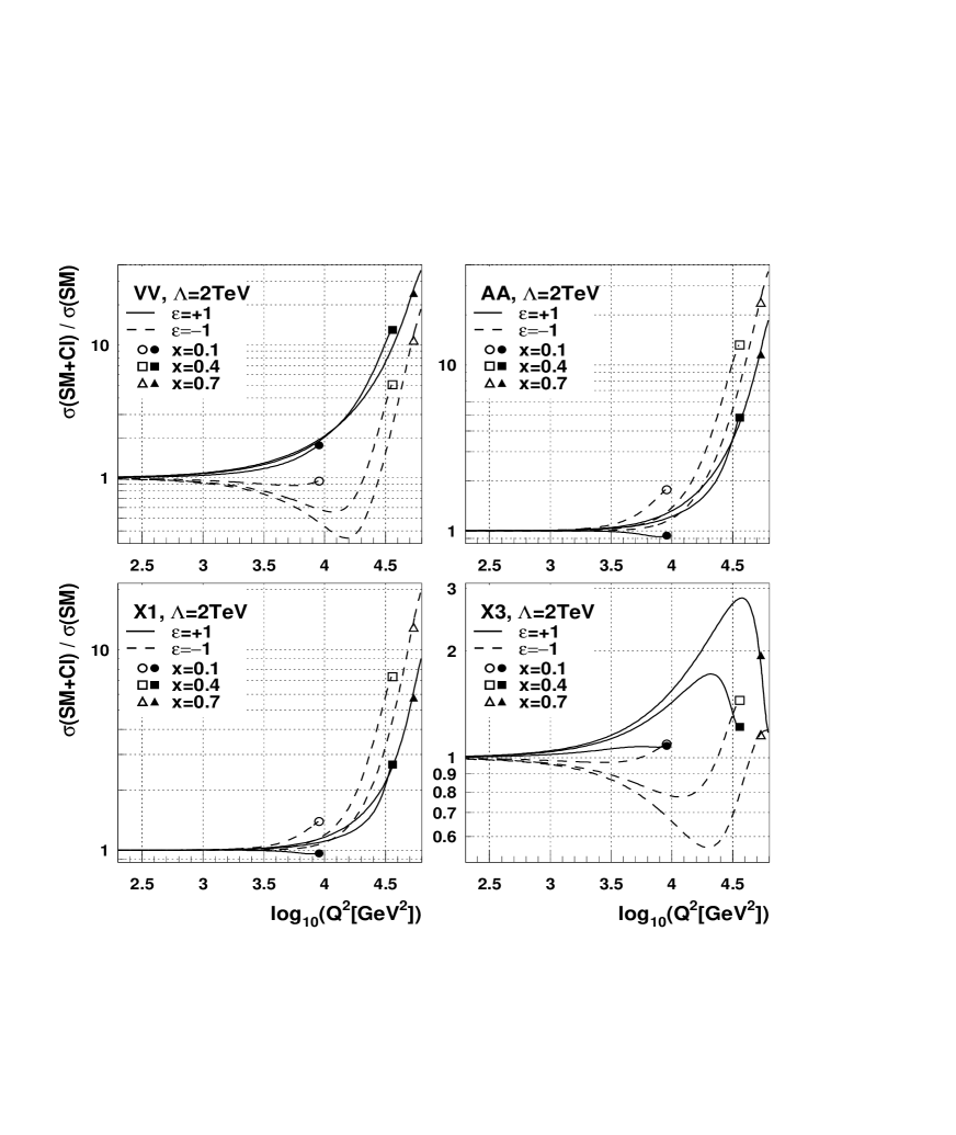
Figure 2: Examples of the relative influence of a CI on the NC DIS cross section $d^{2}\sigma/(dx\,dQ^{2})$ at various fixed values of $x$. The ratio (SM+CI)/SM of differential cross sections for the scenarios VV (top left), AA (top right), X1 (bottom left) and X3 (bottom right) is plotted for $\Lambda=2{\,\text{Te}\kern-0.66666pt\text{V\/}}$. The symbols are used only to label the different curves.

Several examples of modifications of the SM cross sections by CIs are illustrated in Fig. 2. The cross–section modifications for the X1–X6 and the corresponding U1–U6 scenarios are similar, demonstrating that the $d$ quarks have little impact on the CI analysis.

3 Experimental Setup and Data Samples

This analysis uses the data samples, Monte Carlo simulation, event selection, kinematic reconstruction, and assessment of systematic effects used in the NC DIS analysis described in [7]. The data were collected during the years 1994–1997 in $e^{+}p$ collisions with beam energies $E_{e}=27.5{\,\text{Ge}\kern-0.66666pt\text{V\/}}$ and $E_{p}=820{\,\text{Ge}\kern-0.66666pt\text{V\/}}$. The relevant aspects of the experimental setup, event selection, and reconstruction are summarized briefly below. More details can be found in [7].

The ZEUS detector is described in detail elsewhere [27]. The main components used in the present analysis are the central tracking detector (CTD) [28], positioned in a $1.43\,$T solenoidal magnetic field, and the compensating uranium–scintillator sampling calorimeter (CAL) [31], subdivided into forward (FCAL), barrel (BCAL) and rear (RCAL) sections. Under test beam conditions, the CAL energy resolution is $\sigma(E)/E=18\%/\sqrt{E\,[{\text{Ge}\kern-0.66666pt\text{V\/}}]}$ for electrons and $35\%/\sqrt{E\,[{\text{Ge}\kern-0.66666pt\text{V\/}}]}$ for hadrons. A three–level trigger is used to select events online. The trigger decision is based mainly on energies deposited in the calorimeter, specifically on the electromagnetic energy, on the total transverse energy, and on $E-p_{Z}=\sum_{i}E_{i}(1-\cos\theta_{i})$ (the sum running over all calorimeter energy deposits). For fully contained events, the expected value of $E-p_{Z}$ is given by $2E_{e}=55{\,\text{Ge}\kern-0.66666pt\text{V\/}}$. Timing cuts are used to reject beam–gas interactions and cosmic rays.

The luminosity is measured to a precision of $1.6\%$ from the rate of energetic bremsstrahlung photons produced in the process $ep\to ep\gamma$ [35].

The offline event reconstruction applies an algorithm to identify the scattered positron using the topology of its calorimeter signal and the tracking information. The measured energies are corrected for energy loss in inactive material between the interaction point and the calorimeter, for calorimeter inhomogeneities, and for effects caused by redirected hadronic energy from interactions in material between the primary vertex and the calorimeter or by backsplash from the calorimeter (albedo). The kinematic variables for NC DIS candidate events are calculated from the scattering angle of the positron and from an angle representing the direction of the scattered quark. The latter is determined from the transverse momentum and the $E-p_{Z}$ of all energy deposits except those assigned to the scattered positron.

The appropriately corrected experimental quantities are used to make the offline event selection. The major criteria are [7]: (i) the event vertex must be reconstructed from the tracking information, with $|Z_{\rm vtx}|<50\,\text{cm}$; (ii) an isolated scattered positron with energy $E_{e}^{\prime}>10{\,\text{Ge}\kern-0.66666pt\text{V\/}}$ has to be identified; (iii) $38{\,\text{Ge}\kern-0.66666pt\text{V\/}}<E-p_{Z}<65{\,\text{Ge}\kern-0.66666pt\text{V\/}}$; (iv) $y_{e}<0.95$, where $y_{e}$ is the value of $y$ as reconstructed from the measured energy and angle of the scattered $e^{+}$. The requirements (iii) and (iv) reject background events from photoproduction.

Monte Carlo simulations are used to model the expected distributions of the kinematic variables $x$, $y$ and $Q^{2}$ and to estimate the rate of photoproduction background events. NC DIS events including radiative effects are simulated using the heracles 4.5.2 [37] program with the django 6.24 [39] interface to the hadronization programs. In heracles, corrections for initial– and final–state radiation, vertex and propagator corrections, and two–boson exchange are included. The underlying cross sections are calculated in next–to–leading order QCD using the CTEQ4D set [44] of parton distribution functions (PDFs). The NC DIS hadronic final state is simulated using the color–dipole model of ariadne 4.08 [45] and, as a systematic check, the meps option of lepto 6.5 [46] for the QCD cascade. Both programs use the Lund string model of jetset 7.4 [47] for the hadronization. MC samples of photoproduction background events are produced using the herwig 5.8 [50] generator. All MC signal and background events are passed through the detector simulation based on geant [51], incorporating the effects of the trigger. They are subsequently processed with the same reconstruction and analysis programs used for the data. All MC events are weighted to represent the same integrated luminosity as the experimental data.

Good agreement is found in [7] both between the distributions of kinematic variables in data and MC, and between the measured differential cross sections $d\sigma/dQ^{2}$, $d\sigma/dx$ and $d\sigma/dy$ and the respective SM predictions, with the possible exception of the two events at $Q^{2}>35000{\,\text{Ge}\kern-0.66666pt\text{V\/}}^{2}$.

4 Analysis Method

The CI analysis compares the distributions of the measured kinematic variables with the corresponding distributions from a MC simulation of events of the type $e^{+}p\to e^{+}X$, with the weight

$$w=\left.{{d^{2}\sigma\over dx\,dQ^{2}}(\text{SM$+$CI})\over{d^{2}\sigma\over dx\,dQ^{2}}(\text{SM})}\right|_{{\rm true\ }x,y,Q^{2}}$$ (9)

applied to each reconstructed MC event in order to simulate the CI scenarios. The weight $w$ is calculated as the ratio of leading–order cross sections, evaluated at the “true” values of $x$, $y$ and $Q^{2}$ as determined from the four–momentum of the exchanged boson and the beam momenta. In cases where a photon with energy $E_{\gamma}$ is radiated off the incoming positron (initial–state radiation), the $e$ beam energy is reduced by the energy of the radiated photon. The reweighting procedure using eq. (9) accounts correctly for correlations between the effects of a CI signal and the pattern of acceptance losses and migrations.

The simulated background events from photoproduction are added to the selected NC–DIS MC data sets. The photoproduction contamination is highest at high $y$ and is estimated to be less than $0.5\%$ overall and below $3\%$ in any of the bins used for the cross–section measurements in [7].

For each of the CI scenarios, two statistical methods are used. Each incorporates a log–likelihood function

$$L({\epsilon/\Lambda^{2}})=-\sum_{i\in\text{data}}\log{p_{i}({\epsilon/\Lambda^{2}})}\;,$$ (10)

where the $p_{i}$ are appropriately normalized probabilities which are derived from a comparison of measured and simulated event distributions ($i$ runs over individual events in method 1 and over bins of a histogram in method 2, see below). Note that the two CI scenarios corresponding to two sets of $\eta_{mn}^{q}$ values differing only in the overall sign $\epsilon$ are combined into one log–likelihood function. A description of the data samples used for evaluating $L({\epsilon/\Lambda^{2}})$ is given in Table 2 for both methods.

• $\underline{\hbox{Unbinned fit to the $(x,y)$--distribution:\hbox{\vrule height=7.10411pt,depth=2.08818pt,width=0.0pt}}}$

  The available experimental information entering the analysis can be split into two parts, the shape of the $(x,y)$ distribution, $(d^{2}N/dx\,dy)/N_{\rm tot}$, and the total number of events, $N_{\rm tot}$. The latter is related to the total cross section $\sigma_{\rm tot}({\epsilon/\Lambda^{2}})$ in the kinematic region under study by $N_{\rm tot}=\epsilon_{\rm tot}\cdot{\cal L}\cdot\sigma_{\rm tot}$, where $\epsilon_{\rm tot}$ is the average acceptance and ${\cal L}$ denotes the integrated luminosity.

  In the first method, an unbinned log–likelihood technique is applied to calculate $L_{\scriptscriptstyle 1}({\epsilon/\Lambda^{2}})$ from the individual kinematic event coordinates $(x_{i},y_{i})$. This method only makes use of the shape of the $(x,y)$ distribution. The sum in eq. (10) runs over all events in the selected data sample. The MC events are appropriately reweighted to simulate a CI scenario with strength ${\epsilon/\Lambda^{2}}$, as outlined in eq. (9). The probability density $p(x,y;{\epsilon/\Lambda^{2}})$ required to calculate $p_{i}({\epsilon/\Lambda^{2}})=p(x_{i},y_{i};{\epsilon/\Lambda^{2}})$ is determined from the resulting density of MC events in $x$ and $y$ and is normalized to unity, thereby discarding the information on ${\cal L}\cdot\sigma_{\rm tot}({\epsilon/\Lambda^{2}})$. The justification for this deliberate reduction of experimental information is given a posteriori by the fact that $\sigma_{\rm tot}({\epsilon/\Lambda^{2}})$ depends only weakly on $\Lambda$ in the parameter space of interest: for $\Lambda$ values larger than the $95\%$ lower exclusion limits (see Sect. 5), $\sigma_{\rm tot}({\epsilon/\Lambda^{2}})$ deviates from the SM value, $\sigma_{\rm tot}(0)$, by less than $2\%$ for all scenarios except X1 and X6, for which $2.2\%$ and $2.6\%$ are reached, respectively. This sensitivity is smaller than, or of the same order as, the $1.6\%$ systematic luminosity uncertainty quoted in Sect. 3 and is hence not significant.

  Even though $N_{\rm tot}$ is not used in this method, it is important to note that data ($N_{\rm tot}=13243$ events observed) and SM prediction ($13151$ events expected) agree within the luminosity uncertainty and the statistical error. Furthermore, Figs. 4 and 5 demonstrate that the $Q^{2}$ and $x$ distributions agree in shape with the SM expectation. Therefore, a deterioration of the agreement of data and expectation with increasing $|{\epsilon/\Lambda^{2}}|$, indicated by an increase in the log-likelihood function with respect to a minimum close to ${\epsilon/\Lambda^{2}}=0$, can be interpreted in terms of CI exclusion limits on ${\epsilon/\Lambda^{2}}$ or $\Lambda$.

  The sensitivity of the results to systematic effects is studied by repeating the limit setting procedure (see below) for analysis parameters and selection requirements which are varied within admissible ranges. These systematic checks include those which were performed in the underlying cross–section analysis [7]:

  • use of MC samples generated with the meps instead of the ariadne option (as described in Sect. 3);

  • variations of trigger or reconstruction efficiencies and of experimental resolutions within their uncertainties by suitably reweighting the MC events;

  • modifications of the cuts and parameters used for event reconstruction and selection;

  • variation of the calorimeter energy scales in the analysis of the data but not in that of the MC events.

  In addition, systematic uncertainties related to the CI fitting procedure are investigated by

  • use of MC samples which were generated with the following alternatives to the CTEQ4D PDF set: (i) with the PDF set MRSA [52] and (ii) using the results of a recent NLO QCD fit [53] to the 1994 ZEUS [54] and H1 [55] structure function data and to fixed–target data;

  • use of MC samples generated with the PDF sets CTEQ4A2 and CTEQ4A4 [44], corresponding to values of ${\alpha_{s}}(M_{Z}^{2})=0.113$ and $0.119$ (instead of ${\alpha_{s}}(M_{Z}^{2})=0.116$ used for CTEQ4D);

  • changing the amount of photoproduction background in the MC sample by $\pm 100\%$;

  • modifying details of the method used to infer $p(x,y;{\epsilon/\Lambda^{2}})$ from the MC event distributions;

  • calculating the CI cross sections in the following alternative ways:

    • with different parton distribution functions,

    • using NLO instead of LO QCD calculations and parton distributions,

    • with the couplings restricted to first–generation quarks ($\eta_{mn}^{s}\mathchar 61\relax\eta_{mn}^{b}\mathchar 61\relax\eta_{mn}^{c}=0$),

    • with the couplings restricted to first– and second–generation quarks ($\eta_{mn}^{b}\mathchar 61\relax 0$).

  The procedure to determine limits on the CI parameters including the information from the systematic checks is discussed at the end of this section.

• $\underline{\hbox{Binned fit to the $Q^{2}$ distribution:\hbox{\vrule height=7.10411pt,depth=2.08818pt,width=0.0pt}}}$

  In the second method, $L_{\scriptscriptstyle 2}({\epsilon/\Lambda^{2}})$ is determined from the $Q^{2}$ distributions, using Poisson statistics for the numbers of events in each $Q^{2}$ interval. Here, the sum in eq. (10) runs over all $Q^{2}$ bins. For the calculation of $L_{\scriptscriptstyle 2}$, both the shape and the normalization of $dN/dQ^{2}$ are used.

  The systematic uncertainties are included in $L_{\scriptscriptstyle 2}$ using the assumptions that they are fully correlated between bins and that the probability densities for all uncertainties have Gaussian shapes. The effects taken into account are equivalent to those described above for the unbinned method and include in addition a $1.6\%$ uncertainty on the integrated luminosity.

Both methods have been shown to provide unbiased estimates of the CI strength when applied to MC samples. A few examples of comparisons of the resulting log–likelihood functions $L_{\scriptscriptstyle 1}$ and $L_{\scriptscriptstyle 2}$ are shown in Fig. 3. Both functions agree with each other for most of the CI scenarios under study. However, for a few scenarios such as X2^- and X3^-, $L_{\scriptscriptstyle 1}$ rises faster than $L_{\scriptscriptstyle 2}$ with decreasing $\Lambda$. This can be understood as a consequence of the fact that $L_{\scriptscriptstyle 1}$ uses the full two–dimensional information of the $(x,y)$ distribution and is hence more sensitive to those scenarios which imply a marked $x$–dependence of the modification to the cross–section at fixed $Q^{2}$. The two–minimum structure of the log–likelihood functions seen in the AA and X1 scenarios in Fig. 3 is characteristic for several CI scenarios for which the destructive SM$\times$CI interference term cancels approximately the pure CI$\times$CI term in a range of typically $0.1{\,\text{Te}\kern-0.66666pt\text{V\/}}^{-2}\lesssim|{\epsilon/\Lambda^{2}}|\lesssim 0.2{\,\text{Te}\kern-0.66666pt\text{V\/}}^{-2}$. MC studies indicate that the exact shape of $L_{{\scriptscriptstyle 1},{\scriptscriptstyle 2}}$ in the vicinity of these double–minima is dominated by the random pattern of statistical fluctuations of the event distributions, but that the two–dimensional method has a higher probability than the one-dimensional method to assign a larger value of $L$ to the “non–SM minimum” than to the “SM–minimum” (the AA case in Fig. 3 is typical). This is again understood as a consequence of the additional input information for the two–dimensional method. The normalization information, $N_{\rm tot}/({\cal L}\cdot\sigma_{\rm tot}({\epsilon/\Lambda^{2}}))$, cannot distinguish between the minima since the difference of $\sigma_{\rm tot}({\epsilon/\Lambda^{2}})$ between them is much less than the uncertainty of ${\cal L}$.

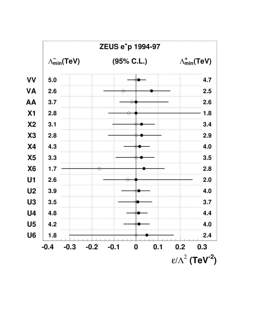
Figure 6: Confidence intervals of $\epsilon/\Lambda^{2}$ at $95\%$ C.L. for all CI scenarios studied in this paper (horizontal bars). The filled (open) circles indicate the positions of the log–likelihood minima, $\epsilon/\Lambda_{\scriptscriptstyle 0}^{2}$, for $\epsilon=+1$ ($\epsilon=-1$). The numbers at the right (left) margin are the lower $\Lambda$ limits for $\epsilon=+1$ ($\epsilon=-1$).

The best estimates, $\Lambda_{\scriptscriptstyle 0}$, for the different CI scenarios are given by the positions of the respective minima of $L_{{\scriptscriptstyle 1},{\scriptscriptstyle 2}}({\epsilon/\Lambda^{2}})$ with $\epsilon=-1$ and $\epsilon=+1$. The values of $\epsilon/\Lambda_{\scriptscriptstyle 0}^{2}$ resulting from the unbinned method are indicated in Fig. 6. Note that $1/\Lambda_{\scriptscriptstyle 0}^{2}=0$ is taken for all cases where $L_{{\scriptscriptstyle 1},{\scriptscriptstyle 2}}({\epsilon/\Lambda^{2}})$ rises monotonically for a given scenario, i.e. for $\epsilon=+1$ or $\epsilon=-1$ (see Fig. 3).

An analysis of the log–likelihood functions (referred to as the “$L$–analysis” in the following) is usually employed to calculate confidence level intervals (i.e. limits) of ${\epsilon/\Lambda^{2}}$. A discussion of some aspects related to the $L$–analysis approach can be found in the Appendix, where polynomial parameterizations for $L_{\scriptscriptstyle 1}({\epsilon/\Lambda^{2}})$ are also provided, which may prove useful for combining our results with those from other experiments. One problem with the $L$–analysis is that its results depend on the choice of the “canonical variable” in terms of which it is performed; for example the $\Lambda$ limits are different if $L$ is evaluated as a function of $\epsilon/\Lambda$ instead of ${\epsilon/\Lambda^{2}}$. In order to avoid this ambiguity, MC experiments (MCE) are used, i.e. statistically independent MC data samples corresponding to the data luminosity. The presence of CIs in the MCEs is simulated by reweighting the events in the MCEs according to eq. (9). For each MCE, the log-likelihood analysis is performed as a function of the assumed “true” value of $\Lambda$, $\Lambda_{\rm true}$, for each of the CI scenarios under study. The lower limit of $\Lambda$ at $95\%$ C.L. for a given CI scenario is determined as the value of $\Lambda_{\rm true}$ at which $95\%$ of the MCEs produce most likely values of $|{\epsilon/\Lambda^{2}}|$ larger than that found in the data. In the cases where $1/\Lambda_{\scriptscriptstyle 0}^{2}\neq 0$, the MCEs are also used to estimate the probability, $p_{\scriptscriptstyle{\rm SM}}$, that a statistical fluctuation in an experiment with the SM cross section would produce a value of $\Lambda_{\scriptscriptstyle 0}$ smaller than that obtained from the data. Note that a high value of $p_{\scriptscriptstyle{\rm SM}}$ does not in itself signify that the SM prediction describes the data well, but indicates that the inclusion of the CI scenario under study does not significantly improve the agreement between data and prediction.

For the two–dimensional fitting method, the above procedure is repeated for each systematic check, using statistically independent MCE sets which reflect the corresponding modifications of the analysis. Each such MCE set consists of $500$ MCEs. The resulting CI limits are scattered around the limits of the central analysis, with deviations in both directions being about equally frequent. The $\Lambda$ limits deviate from their central values by typically less than $15\%$, though by as much as $30\%$ in a few cases. The modification of the underlying SM cross section induced by a variation of ${\alpha_{s}}(M_{Z}^{2})$ and by using different PDF sets (see above) causes variations of the $\Lambda$ limits of typically a few percent and $25\%$ maximally.

Systematic effects are finally taken into account in the CI limit analysis by combining the MCE sets of all systematic checks and determining the values of $\Lambda_{\rm true}$ for which $95\%$ of all MCEs in the combined set produce most likely values of $|{\epsilon/\Lambda^{2}}|$ larger than that found in the data. This procedure is an approximation to averaging over the spectra of systematic effects, assuming that the different checks are uncorrelated and that the ranges of parameter variations (e.g. of the calorimeter energy scales or of ${\alpha_{s}(M_{Z}^{2})}$) reflect the actual uncertainties. The corresponding question defining a $95\%$ C.L. limit is: “which value of $\Lambda_{\rm true}$ causes deviations from the SM prediction which are larger than that observed in the experimental data in $95\%$ of all ZEUS–type experiments exhibiting systematic differences according to the spectra determined in the analysis of systematic effects”.

The $\Lambda$ limits resulting from both log–likelihood methods agree to within $15\%$ in all cases except for the scenarios AA⁺, X2^- and X3^-, for which the two–dimensional method has higher sensitivity and correspondingly yields significantly stronger limits. Therefore, the results of this method are presented in the following.

5 Results

The resulting SM probabilities $p_{\scriptscriptstyle{\rm SM}}$ (see Table 3) do not indicate significant amplitudes for any of the CI scenarios considered. Therefore, we report upper limits on $1/\Lambda^{2}$ and the corresponding lower limits on $\Lambda$.

A selection of plots demonstrating the expected modifications of the $Q^{2}$– and $x$–distributions in the presence of CIs with strengths corresponding to the $95\%$ C.L. exclusion limits is shown in Figs. 4 and 5. As mentioned in Sect. 1, the data show an excess over the SM predictions at $Q^{2}\gtrsim 35000{\,\text{Ge}\kern-0.66666pt\text{V\/}}^{2}$. However, it is apparent that CIs cannot provide an improved description of this excess while simultaneously describing the data well at lower $Q^{2}$, where data and SM expectation are in good agreement. These figures also confirm that the $x$–dependence of the (SM+CI)/SM cross–section ratio differs markedly between different CI scenarios and obviously contributes to the sensitivity of the CI fit, e.g. in the X3 case. This statement is generally true for all cases where the limits derived from the two analysis methods differ significantly.

The lower limits on $\Lambda$ ($\Lambda^{\pm}_{\rm lim}$) and the probabilities $p_{\scriptscriptstyle{\rm SM}}$ are summarized in Table 3 and are displayed in Fig. 6. In none of the cases does the SM probability fall below $16\%$. The $\Lambda$ limits range from $1.7{\,\text{Te}\kern-0.66666pt\text{V\/}}$ to $5{\,\text{Te}\kern-0.66666pt\text{V\/}}$. Those few cases with limits below $2.5{\,\text{Te}\kern-0.66666pt\text{V\/}}$ correspond to log–likelihood functions having a broad minimum, either in the region with $\epsilon=+1$ (X1, U1) or with $\epsilon=-1$ (X6, U6); these minima correspond to parameter combinations for which the pure CI$\times$CI contribution and the CI$\times$SM interference term approximately cancel in the HERA kinematic regime.

Table 4 shows a comparison of the ZEUS CI results with corresponding limits reported recently by other experiments which study $eeqq$ CIs in $e^{+}e^{-}$ scattering at LEP (ALEPH [9], L3 [12], OPAL [15]) or via Drell–Yan pair production in $p\mkern 1.5mu\overline{\mkern-1.5mup\mkern-1.0mu}\mkern 1.0mu$ scattering (CDF [16], DØ [17]). The H1 [8] and DELPHI [10] collaborations report results only for purely chiral CIs which cannot be compared to the results of this paper. All limits shown in Table 4 have been derived assuming flavor symmetry (see eq. (7)), except the LEP limits for the U3 and U4 scenarios which are for first–generation quarks only. Limits for the X2, X5, U1, U2, U5 and U6 scenarios are not included in Table 4 because there exist no previously published results. ZEUS and the other experiments are all sensitive to CIs at mass scales of a few  TeV. The relative sensitivity to different CI scenarios depends on the CI$\times$SM interference sign which is opposite in $e^{+}p$ scattering on the one hand and in $e^{+}e^{-}$ and $p\mkern 1.5mu\overline{\mkern-1.5mup\mkern-1.0mu}\mkern 1.0mu$ scattering on the other. Where available, the LEP limits often exceed the results of this paper, although it should be noted that this depends on the assumption of a flavor–symmetric CI structure. Limits for CIs which couple only to first–generation quarks would differ only by a small amount from those reported here for $ep$ or $p\mkern 1.5mu\overline{\mkern-1.5mup\mkern-1.0mu}\mkern 1.0mu$ scattering, but would be significantly weaker in the case of LEP.

6 Conclusions

We have searched for indications of $eeqq$ contact interactions in $47.7\,\text{pb}^{-1}$ of ZEUS high–$Q^{2}$ $e^{+}p$ neutral–current deep inelastic scattering data. The distributions of the kinematic variables in the data have been compared to predictions derived for 30 scenarios of vector contact interactions which differ in their helicity structure and quark–flavor dependence. In none of the cases has a significant indication of a contact interaction been found and $95\%$ C.L. upper limits on $1/\Lambda^{2}$ have been determined for each of these scenarios. The lower limits on $\Lambda$ range between $1.7{\,\text{Te}\kern-0.66666pt\text{V\/}}$ and $5{\,\text{Te}\kern-0.66666pt\text{V\/}}$ and are found to be largely independent of the statistical method applied.

The results exhibit a sensitivity to contact interactions similar to that recently reported by other experiments; in order to allow full use to be made of the available experimental data, the information needed to combine the results of this analysis with those from other sources is provided. Some of the limits reported here are the most restrictive yet published, and several of the contact–interaction scenarios have been studied in this paper for the first time.

Acknowledgments: We appreciate the contributions to the construction and maintenance of the ZEUS detector by many people who are not listed as authors. We especially thank the DESY computing staff for providing the data analysis environment and the HERA machine group for their outstanding operation of the collider. Finally, we thank the DESY directorate for strong support and encouragement.

This paper was completed shortly after the tragic and untimely death of Prof. Dr. B. H. Wiik, Chairman of the DESY directorate. All members of the ZEUS collaboration wish to acknowledge the remarkable rôle which he played in the success of both the HERA project and of the ZEUS experiment. His inspired scientific leadership, his warm personality and his friendship will be sorely missed by us all.

Appendix: The Log–Likelihood Functions

In this Appendix we summarize some aspects of interpreting the log–likelihood functions $L({\epsilon/\Lambda^{2}})$ using a Bayesian probabilistic approach. The results of the unbinned method described in Sect. 4 have been employed here, but systematic effects have not been taken into account. For simplicity, we will denote the log–likelihood functions by $L$ instead of $L_{\scriptscriptstyle 1}$ in this Appendix.

For ease of calculation, the functions $L({\epsilon/\Lambda^{2}})-L_{\rm min}$ have been parameterized as eighth–order polynomials in the region where $L({\epsilon/\Lambda^{2}})-L_{\rm min}<18$, corresponding approximately to a $\pm 6\sigma$ interval around the minimum of $L$. The polynomial coefficients are summarized in Table 5. The accuracy of the parameterizations is typically better than $0.1$ units in $L$. Note that, neglecting systematic effects, these parameterizations allow one to combine the ZEUS results with those of other experiments by simply adding the $L$ functions and repeating the analysis described below.

The Bayesian approach starts from the relation

$$p({\epsilon/\Lambda^{2}}|{\cal D})\propto p({\cal D}|{\epsilon/\Lambda^{2}})\cdot p_{\scriptscriptstyle 0}({\epsilon/\Lambda^{2}})\;,$$ (11)

where ${\cal D}$ symbolizes the experimental data, $p({\cal D}|{\epsilon/\Lambda^{2}})$ is the conditional probability to observe ${\cal D}$ for a given value of ${\epsilon/\Lambda^{2}}$, and $p_{\scriptscriptstyle 0}({\epsilon/\Lambda^{2}})$ is the prior probability describing the knowledge about ${\epsilon/\Lambda^{2}}$ before the experiment was conducted. The probability $p({\epsilon/\Lambda^{2}}|{\cal D})$ assigned to ${\epsilon/\Lambda^{2}}$ under the condition of having observed ${\cal D}$ is what we actually want to derive.

In the following, we will identify

$$p({\cal D}|{\epsilon/\Lambda^{2}})\propto{\rm exp}\left(-L({\epsilon/\Lambda^{2}})\right)\;,$$ (12)

with the normalization appropriately fixed to unity. In the simplest case of a Gaussian probability distribution, $L({\epsilon/\Lambda^{2}})$ is a parabola, and $\sigma_{{\epsilon/\Lambda^{2}}}$, the RMS width of $p({\cal D}|{\epsilon/\Lambda^{2}})$, corresponds to the width of the Gaussian. Even though some of the $L({\epsilon/\Lambda^{2}})$ functions of the CI analysis are not parabola–like, $\sigma_{{\epsilon/\Lambda^{2}}}$ is still well defined and can be interpreted as a measure of the experimental sensitivity to a given CI scenario. The values of $\sigma_{{\epsilon/\Lambda^{2}}}$ are summarized in Table 3.

Usually, simple assumptions about $p_{\scriptscriptstyle 0}({\epsilon/\Lambda^{2}})$ are made in order to calculate $p({\epsilon/\Lambda^{2}}|{\cal D})$, which only weakly depends on these assumptions provided that the width of $p_{\scriptscriptstyle 0}({\epsilon/\Lambda^{2}})$ is much larger than $\sigma_{{\epsilon/\Lambda^{2}}}$. We have calculated $p({\epsilon/\Lambda^{2}}|{\cal D})$ using a flat prior probability restricted to either $\epsilon\geq 0$ or $\epsilon\leq 0$. One–sided $95\%$ C.L. limits in the Bayesian approach ($\Lambda^{\pm}_{\rm lim,B}$) have been determined by solving

$${\int\limits_{0}^{1/(\Lambda^{+}_{\rm lim,B})^{2}}\;d\xi\,{\rm exp}\left(-L(\xi)\right)\over\int\limits_{0}^{\infty}\;d\xi\,{\rm exp}\left(-L(\xi)\right)}=0.95\quad\text{and}\quad{\int\limits_{-1/(\Lambda^{-}_{\rm lim,B})^{2}}^{0}\;d\xi\,{\rm exp}\left(-L(\xi)\right)\over\int\limits_{-\infty}^{0}\;d\xi\,{\rm exp}\left(-L(\xi)\right)}=0.95\;;$$ (13)

For all CI scenarios, the results deviate by less than $20\%$ from the limits $\Lambda_{\rm lim}$ resulting from the MCE method (see Sect. 4). Note that systematic effects have not been considered for this cross check.

An alternative way to present the results of this search analysis is obtained by considering the ratio of two equations of the type (11) for different values of ${\epsilon/\Lambda^{2}}$, where one is taken as a reference value (chosen to be ${\epsilon/\Lambda^{2}}=0$, i.e. corresponding to the SM). Rearranging the terms yields

$$\left.{p({\epsilon/\Lambda^{2}}|{\cal D})\over p_{\scriptscriptstyle 0}({\epsilon/\Lambda^{2}})}\right/{p({\epsilon/\Lambda^{2}}=0|{\cal D})\over p_{\scriptscriptstyle 0}({\epsilon/\Lambda^{2}}=0)}={p({\cal D}|{\epsilon/\Lambda^{2}})\over p({\cal D}|{\epsilon/\Lambda^{2}}=0)}=R({\epsilon/\Lambda^{2}})\;,$$ (14)

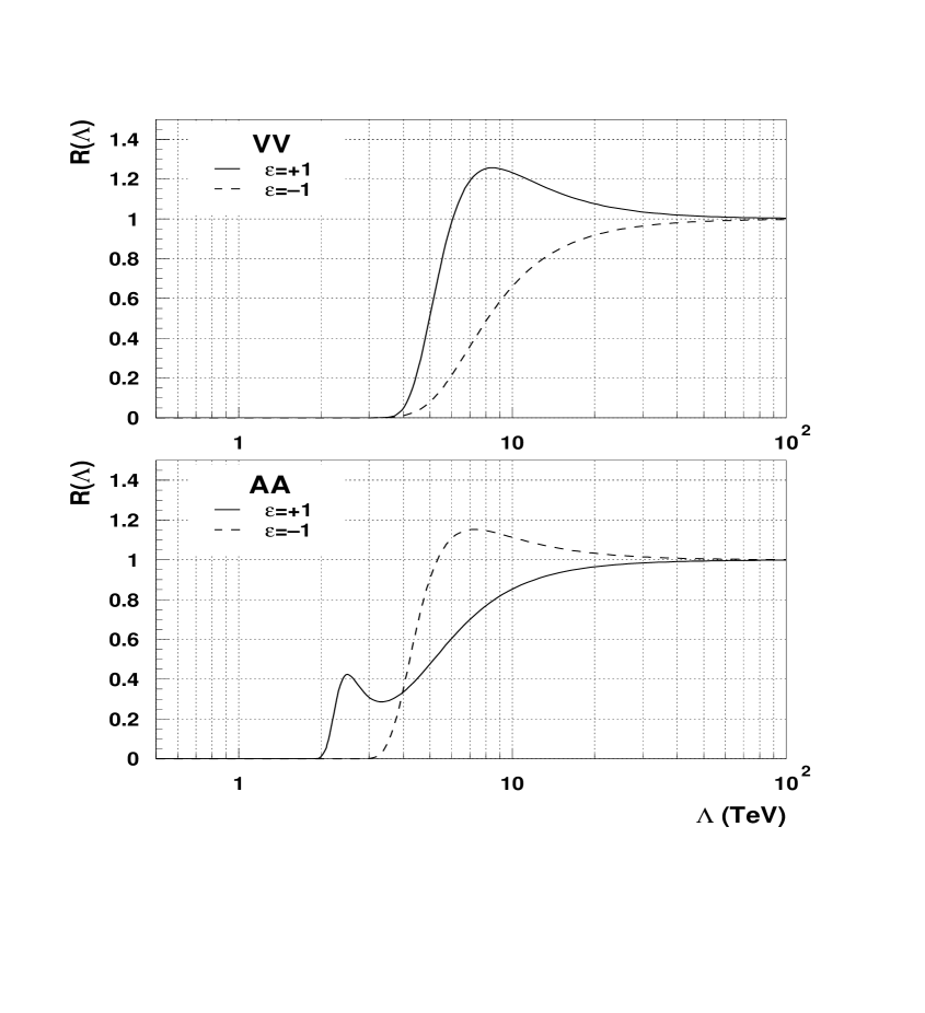
Figure 7: The function $R$ defined in eq. (14) for the VV (top) and the AA (bottom) scenarios, for $\epsilon=+1$ (solid lines), and for $\epsilon=-1$ (dashed lines). The graphs are based on the polynomial parameterizations of Table 5.

where the double ratio on the left–hand side quantifies how the probability assigned to a given value of ${\epsilon/\Lambda^{2}}$ changes due to the experimental data ${\cal D}$, with the reference point, ${\epsilon/\Lambda^{2}}=0$, fixing the normalization. The function $R({\epsilon/\Lambda^{2}})$ has been discussed in detail elsewhere (see e.g. [56] and references therein). The representation of eq. (14) is independent of the prior probability and can be used to combine the results of this analysis with those of other experiments by analyzing the product of corresponding $R$ functions. Note that $R$ does not involve integrations over ${\epsilon/\Lambda^{2}}$ and is hence invariant with respect to the variable transformations mentioned in Sect. 4; in particular, $R$ can be interpreted both as a function of ${\epsilon/\Lambda^{2}}$ and as a function of $\Lambda$. By definition, $R$ asymptotically approaches unity if ${\epsilon/\Lambda^{2}}\to 0$ or $\Lambda\to\infty$, indicating the loss of experimental sensitivity as the CI strength vanishes. Regions where $R$ is close to zero are excluded by ${\cal D}$, whereas $R>1$ indicates “signal–type” regions where the experimental data are better described by a CI scenario than by the SM. Typical $R$ values for significant deviations from the SM are expected to exceed unity by several orders of magnitude (cf. the discussion in [56]). Two representative examples of the functions $R(\Lambda)$ observed in the CI analysis are shown in Fig. 7. In none of the scenarios from Table 2 does $R$ exceed unity by more than $40\%$, corroborating the conclusion that there is no significant indication for the presence of CIs. The threshold–type region of $R(\Lambda)$ indicates the position of the $\Lambda$ limit. Indeed one obtains limits similar to those reported in Sect. 5 by solving the condition $R(\Lambda^{\pm}_{\rm lim,R})=0.05$ for $\Lambda^{\pm}_{\rm lim,R}$.

Label	$\eta^{u}_{LL}$	$\eta^{u}_{LR}$	$\eta^{u}_{RL}$	$\eta^{u}_{RR}$	$\eta^{d}_{LL}$	$\eta^{d}_{LR}$	$\eta^{d}_{RL}$	$\eta^{d}_{RR}$
VV	$+1$	$+1$	$+1$	$+1$	$+1$	$+1$	$+1$	$+1$
AA	$+1$	$-1$	$-1$	$+1$	$+1$	$-1$	$-1$	$+1$
VA	$+1$	$-1$	$+1$	$-1$	$+1$	$-1$	$+1$	$-1$
X1	$+1$	$-1$	$0$	$0$	$+1$	$-1$	$0$	$0$
X2	$+1$	$0$	$+1$	$0$	$+1$	$0$	$+1$	$0$
X3	$+1$	$0$	$0$	$+1$	$+1$	$0$	$0$	$+1$
X4	$0$	$+1$	$+1$	$0$	$0$	$+1$	$+1$	$0$
X5	$0$	$+1$	$0$	$+1$	$0$	$+1$	$0$	$+1$
X6	$0$	$0$	$+1$	$-1$	$0$	$0$	$+1$	$-1$
U1	$+1$	$-1$	$0$	$0$	$0$	$0$	$0$	$0$
U2	$+1$	$0$	$+1$	$0$	$0$	$0$	$0$	$0$
U3	$+1$	$0$	$0$	$+1$	$0$	$0$	$0$	$0$
U4	$0$	$+1$	$+1$	$0$	$0$	$0$	$0$	$0$
U5	$0$	$+1$	$0$	$+1$	$0$	$0$	$0$	$0$
U6	$0$	$0$	$+1$	$-1$	$0$	$0$	$0$	$0$

Table 1: The 30 scenarios for contact interactions considered in this paper. Each row of this table corresponds to two different CI scenarios for overall interference signs $\epsilon=+1$ and $\epsilon=-1$, respectively (see eq. (1) in the text).

quantity	method 1	method 2
$Q^{2}_{\rm min}\;({\text{Ge}\kern-0.66666pt\text{V\/}}^{2})$	${\phantom{00}}500$	${\phantom{00}}400$
$Q^{2}_{\rm max}\;({\text{Ge}\kern-0.66666pt\text{V\/}}^{2})$	$90200$	$51200$
$x_{\rm min}$	$0.04$	—
$x_{\rm max}$	$0.95$	—
$y_{\rm min}$	$0.04$	—
$y_{\rm max}$	$0.95$	—
events	$13243$	$37379$

Table 2: The kinematic regions used for the CI analysis in the two fitting methods. Note that the cuts on $Q^{2}$, $x$, and $y$ indicated in the table are applied in addition to the event selection criteria described in Sect. 3.

$\epsilon=-1$ $\epsilon=+1$ CI $\Lambda^{-}_{\rm lim}$ $p_{\scriptscriptstyle{\rm SM}}$ $\Lambda^{+}_{\rm lim}$ $p_{\scriptscriptstyle{\rm SM}}$ $\sigma_{{\epsilon/\Lambda^{2}}}$ $({\text{Te}\kern-0.66666pt\text{V\/}})$ $({\text{Te}\kern-0.66666pt\text{V\/}})$ ${\text{Te}\kern-0.66666pt\text{V\/}}^{-2}$ VV 5.0 4.7 0.28 0.021 VA 2.6 0.25 2.5 0.25 0.070 AA 3.7 0.28 2.6 0.080 X1 2.8 0.26 1.8 0.113 X2 3.1 3.4 0.28 0.056 X3 2.8 2.9 0.37 0.066 X4 4.3 4.0 0.26 0.034 X5 3.3 3.5 0.28 0.052 X6 1.7 0.16 2.8 0.27 0.105 U1 2.6 0.24 2.0 0.125 U2 3.9 4.0 0.38 0.037 U3 3.5 3.7 0.48 0.046 U4 4.8 4.4 0.32 0.025 U5 4.2 4.0 0.36 0.032 U6 1.8 2.4 0.24 0.118

Table 3: Values of the $95\%$ C.L. limits ($\Lambda^{\pm}_{\rm lim}$) for all CI scenarios, as well as the SM probabilities, $p_{\scriptscriptstyle{\rm SM}}$, for those scenarios with $\epsilon/\Lambda_{\scriptscriptstyle 0}^{2}\neq 0$ (see Sect. 4). In the last column, the RMS width of the probability distribution $p_{L}\propto{\rm exp}(-L({\epsilon/\Lambda^{2}}))$ is indicated (cf. Appendix).

	$\Lambda^{\pm}_{\rm lim}\;({\text{Te}\kern-0.66666pt\text{V\/}})$ ($95\%$ C.L.)
CI	ZEUSa	ALEPH	L3	OPAL	CDF	DØ
	this	[9]	[12]	[15]	[16]	[17]
	study		prelim.
VV$+$	4.7	6.4	3.8	4.1	3.5	4.9
VV$-$	5.0	7.1	5.0	5.7	5.2	6.1
AA$+$	2.6	7.2	5.6	6.3	3.8	4.7
AA$-$	3.7	7.9	3.5	3.8	4.8	5.5
X1$+$	1.8	—	—	—	—	3.9
X1$-$	2.8	—	—	—	—	4.5
X3$+$	2.9	6.7	4.0	4.4	—	4.2
X3$-$	2.8	7.4	3.4	3.8	—	5.1
X4$+$	4.0	2.9	2.9	3.1	—	3.9
X4$-$	4.3	4.5	4.8	5.5	—	4.4
X6$+$	2.8	—	—	—	—	4.0
X6$-$	1.7	—	—	—	—	4.3
U3$+$	3.7	—	6.1	4.1	—	—
U3$-$	3.5	—	4.9	5.8	—	—
U4$+$	4.4	—	2.1	2.3	—	—
U4$-$	4.8	—	2.9	3.2	—	—

^a No comparison is made for scenarios for which only ZEUS sets limits: X2, X5, U1, U2, U5, U6.

Table 4: Lower $\Lambda$ limits at $95\%$ C.L. from this study compared to equivalent results from other experiments. The results of the L3 collaboration are preliminary. The X1, X3/U3, X4/U4, and X6 scenarios are denoted LL–LR, LL+RR or V0, LR+RL or A0, and RL–RR, respectively, by the LEP and Tevatron experiments. Note that CDF also provides limits for $\mu\mu qq$ CI (not shown here) which can be combined with the $eeqq$ limits if one assumes lepton flavor universality.

CI $\lambda_{0}$ $\lambda_{1}$ $\lambda_{2}$ $\lambda_{3}$ $\lambda_{4}$ scenario $\lambda_{5}$ $\lambda_{6}$ $\lambda_{7}$ $\lambda_{8}$ VV 0.219960 –0.317192+2 0.102541+4 0.559212+4 –0.157739+5 –0.171440+6 0.296531+6 0.381829+7 0.604081+7 VA 0.245590 0.137604+1 –0.977350+2 –0.345909+3 0.131860+5 0.684982+4 –0.160571+6 –0.532035+5 0.948424+6 AA 0.241619 0.136626+2 0.255357+3 –0.361006+4 0.477991+4 0.549759+5 –0.700729+5 –0.431092+6 0.831623+6 X1 0.206150 0.700878+1 0.510132+2 –0.102610+4 0.197029+4 0.829875+4 –0.124916+5 –0.338700+5 0.571381+5 X2 0.198413 –0.113778+2 0.181979+3 0.126775+4 0.163454+4 –0.100860+5 –0.147490+5 0.448248+5 0.807606+5 X3 0.082637 –0.608908+1 0.109116+3 0.214284+3 0.131258+3 –0.396591+3 –0.110789+3 0.692834+3 0.517102+3 X4 0.327244 –0.213799+2 0.470532+3 0.356225+4 0.558752+3 –0.519826+5 –0.454742+5 0.362723+6 0.623043+6 X5 0.258595 –0.142310+2 0.218532+3 0.147937+4 0.816187+3 –0.134481+5 –0.960868+4 0.720345+5 0.103106+6 X6 0.143683 –0.486270+1 0.280939+2 0.843126+3 0.235808+4 –0.623902+4 –0.141521+5 0.234297+5 0.505643+5 U1 0.277925 0.822634+1 0.581735+2 –0.708590+3 0.828391+3 0.476597+4 –0.472480+4 –0.158164+5 0.208190+5 U2 0.086540 –0.100733+2 0.350929+3 0.100296+4 0.118597+3 –0.122795+5 –0.957897+4 0.960528+5 0.159882+6 U3 0.016648 –0.397315+1 0.241440+3 0.103296+3 –0.139481+3 –0.115302+2 0.154464+3 –0.851289+2 0.437650+3 U4 0.145224 –0.224785+2 0.824204+3 0.231869+4 –0.154694+5 –0.237649+5 0.454907+6 0.537245+5 –0.486230+7 U5 0.108391 –0.149704+2 0.498695+3 0.981530+3 –0.449846+4 –0.546963+4 0.877442+5 0.215059+3 –0.652759+6 U6 0.174813 –0.417751+1 0.981713+1 0.462709+3 0.134709+4 –0.284097+4 –0.650313+4 0.835725+4 0.172630+5

Table 5: Parameterizations of the functions $L({\epsilon/\Lambda^{2}})-L_{\rm min}$ resulting from the unbinned method. For each CI scenario, the nine coefficients $\lambda_{i}$ define a polynomial $\sum_{i=0}^{8}\lambda_{i}({\epsilon/\Lambda^{2}})^{i}$ which has been fitted to $L({\epsilon/\Lambda^{2}})-L_{\rm min}$ in the range where $L({\epsilon/\Lambda^{2}})-L_{\rm min}<18$. The notation $x\mathchar 43\relax n$ is used as a shorthand for $x\cdot 10^{n}$.

Figure 1: The Feynman diagram for an $eeqq$ contact interaction.

Figure 3: Log–likelihood as a function of $\epsilon/\Lambda^{2}$ as obtained by the two methods described in Sect. 4, for the scenarios VV (top left), AA (top right), X1 (bottom left), and X3 (bottom right). For both methods, the values of $L-L_{\rm min}$ are shown. Note that the two methods use different statistical approaches and, in addition, differ in their treatment of systematic effects. Each figure represents two CI scenarios ($\epsilon=+1$, $\epsilon=-1$).

Figure 4: Exclusion limits on CI strengths in terms of the corresponding modification of the expected distributions of $Q^{2}$ (left) and $x$ (right) in the kinematic region used for method 1 (see Sect. 4 and Table 2). The dots represent the ratios of observed and expected numbers of events and the error bars indicate the statistical uncertainties. The histograms show the modification of this ratio for the VV (top) and AA (bottom) scenarios as obtained with the $\Lambda_{\rm lim}$ values given in Table 3. The solid (dotted) line corresponds to the $95\%$ exclusion limit for $\epsilon=+1$ ($\epsilon=-1$).

Figure 5: Exclusion limits on CI strengths in terms of the corresponding modification of the expected distributions of $Q^{2}$ (left) and $x$ (right) in the kinematic region used for method 1 (see Sect. 4 and Table 2). The dots represent the ratios of observed and expected numbers of events and the error bars indicate the statistical uncertainties. The histograms show the modification of this ratio for the X1 (top) and X3 (bottom) scenarios as obtained with the $\Lambda_{\rm lim}$ values given in Table 3. The solid (dotted) line corresponds to the $95\%$ exclusion limit for $\epsilon=+1$ ($\epsilon=-1$).

References

- [1] ZEUS Collaboration, J. Breitweg et al., Z. Phys. C 74 (1997) 207
- [2] H1 Collaboration, C. Adloff et al., Z. Phys. C 74 (1997) 191
- [3] G. Altarelli et al., Nucl. Phys. B 506 (1997) 3
- [4] V. Barger et al., Phys. Lett. B 404 (1997) 147
- [5] V. Barger et al., Phys. Rev. D 57 (1998) 391
- [6] N. Di Bartolomeo and M. Fabbrichesi, Phys. Lett. B 406 (1997) 237
- [7] ZEUS Collaboration, J. Breitweg et al., Eur. Phys. J. C 11 (1999) 427
- [8] H1 Collaboration, S. Aid et al., Phys. Lett. B 353 (1995) 578
- [9] ALEPH Collaboration, R. Barate et al., Preprint CERN–EP/99–042, CERN (1999), hep-ex/9904011, subm. to Eur. Phys. J
- [10] DELPHI Collaboration, P. Abreu et al., Eur. Phys. J. C 11 (1999) 383
- [11] L3 Collaboration, M. Acciarri et al., Phys. Lett. B 433 (1998) 163
- [12] L3 Collaboration, submitted paper 513 to XXIX International Conference on High Energy Physics, Vancouver, July 23–29, 1998
- [13] D. Bourilkov, Preprint ETHZ–IPP PR–98–02, ETH Zürich (1998), hep-ex/9806027
- [14] D. Bourilkov, private communication
- [15] OPAL Collaboration, G. Abbiendi et al., Eur. Phys. J. C 6 (1999) 1
- [16] CDF Collaboration, F. Abe et al., Phys. Rev. Lett. 79 (1997) 2198
- [17] DØ Collaboration, D. Abbott et al., Phys. Rev. Lett. 82 (1999) 4769
- [18] E. Fermi, Z. Phys. 88 (1934) 161
- [19] E. Fermi, Nuovo Cimento 11 (1934) 1
- [20] P. Haberl, F. Schrempp and H. U. Martyn, in Proc. Workshop Physics at HERA, ed. W. Buchmüller and G. Ingelman, Hamburg, Germany, 1991, p. 1133
- [21] E. Eichten, K. Lane and M. Peskin, Phys. Rev. Lett. 50 (1983) 811
- [22] R. Rückl, Phys. Lett. 129 B (1983) 363
- [23] R. Rückl, Nucl. Phys. B 234 (1984) 91
- [24] C. S. Wood et al., Science 275 (1997) 1759
- [25] A. Deandrea, Phys. Lett. B 409 (1997) 277
- [26] L. Giusti and A. Strumia, Phys. Lett. B 410 (1997) 229
- [27] ZEUS Collaboration, ed. U. Holm, Status Report, 1993
- [28] N. Harnew et al., Nucl. Instrum. Methods A 279 (1989) 290
- [29] B. Foster et al., Nucl. Phys. B (Proc. Suppl.) 32 (1993) 181
- [30] B. Foster et al., Nucl. Instrum. Methods A 338 (1994) 254
- [31] M. Derrick et al., Nucl. Instrum. Methods A 309 (1991) 77
- [32] ZEUS Calorimeter group, A. Andresen et al., Nucl. Instrum. Methods A 309 (1991) 101
- [33] A. Caldwell et al., Nucl. Instrum. Methods A 321 (1992) 356
- [34] A. Bernstein et al., Nucl. Instrum. Methods A 336 (1993) 23
- [35] J. Andruszków et al., Report DESY–92–066, DESY (1992)
- [36] ZEUS Collaboration, M. Derrick et al., Z. Phys. C 63 (1994) 391
- [37] A. Kwiatkowski, H. Spiesberger and H.–J. Möhring, Comp. Phys. Commun. 69 (1992) 155
- [38] H. Spiesberger, heracles. An Event Generator for Interactions at HERA Including Radiative Processes (Version 4.6), 1996, available on WWW: http://www.desy.de/~hspiesb/heracles.html
- [39] K. Charchuła, G. A. Schuler and H. Spiesberger, Comp. Phys. Commun. 81 (1994) 381
- [40] H. Spiesberger, django6 version 2.4 — A Monte Carlo Generator for Deep Inelastic Lepton Proton Scattering Including QED and QCD Radiative Effects, 1996, available on WWW: http://www.desy.de/~hspiesb/django6.html
- [41] CTEQ Collaboration, H.L. Lai et al., Preprint MSU–HEP–903100, Michigan State Univ. (1999), hep–ph/9903282, subm. to Eur. Phys. J
- [42] A. D. Martin et al., Eur. Phys. J. C 4 (1998) 463
- [43] A. D. Martin et al., in Proc. 7th Int. Workshop on Deep Inelastic Scattering (DIS99), Zeuthen, Germany, 1999, hep–ph/9906231
- [44] CTEQ Collaboration, H. L. Lai et al., Phys. Rev. D 55 (1997) 1280
- [45] L. Lönnblad, Comp. Phys. Commun. 71 (1992) 15
- [46] G. Ingelman, A. Edin and J. Rathsman, Comp. Phys. Commun. 101 (1997) 108
- [47] T. Sjöstrand, Comp. Phys. Commun. 39 (1986) 347
- [48] T. Sjöstrand and M. Bengtsson, Comp. Phys. Commun. 43 (1987) 367
- [49] T. Sjöstrand, Comp. Phys. Commun. 82 (1994) 74
- [50] G. Marchesini et al., Comp. Phys. Commun. 67 (1992) 465
- [51] R. Brun et al., Report CERN–DD/EE/84–1, CERN (1987)
- [52] A. D. Martin, W. J. Stirling and R. G. Roberts, Phys. Rev. D 51 (1995) 4756
- [53] M. Botje, Preprint DESY–99–038, DESY (1999), hep-ph/9912439
- [54] ZEUS Collaboration, M. Derrick et al., Z. Phys. C 72 (1996) 399
- [55] H1 Collaboration, S. Aid et al., Nucl. Phys. B 470 (1996) 3
- [56] G. D’Agostini and G. Degrassi, Eur. Phys. J. C 10 (1999) 663.