OUNP-99-05 PDK-730 The Observation of a Shadow of the Moon in the Underground Muon Flux in the Soudan 2 Detector.
The Soudan 2 Collaboration

Abstract

A shadow of the moon, with a statistical significance of $5\sigma$, has been observed in the underground muon flux at a depth of 2090 mwe using the Soudan 2 detector. The angular resolution of the detector is well described by a Gaussian with a sigma $\leq 0.3^{\circ}$. The position of the shadow confirms that the alignment of the detector is known to better than $0.15^{\circ}$ and has remained stable during ten years of data taking.

Submitted to Physical Review D

I Introduction

The Soudan 2 detector is a 963 tonne iron and drift-tube sampling calorimeter, designed to search for nucleon decay [1, 2], situated in the Soudan mine in northern Minnesota, USA. The spatial resolution of the detector is $<1$ cm in three dimensions. Throughgoing muons are typically reconstructed with track lengths of a few metres and the angular resolution for such tracks is expected to be a fraction of a degree. Because of the good angular resolution and the uniform exposure of the detector over the period of ten years from January 1989, the detector is excellently suited to a study of the possible existence of point sources of underground muons.

A prerequisite for such a search is a thorough understanding of the alignment and angular resolution (point spread function or psf) of the detector. The angular diameters of the moon and sun are both $\sim 0.5^{\circ}$. Both objects will occlude the high energy cosmic ray primaries responsible for the underground muon flux. Since their angular sizes are small and comparable with the psf of the detector the observation of shadows in the underground muon flux will confirm both the alignment and the angular resolution of the detector.

The potential observation of moon and sun shadows with high energy cosmic rays was originally suggested by Clark [3]; the observation of the effect of the solar magnetic field on the cosmic ray shadow of the sun has been suggested as a means of determining the composition of primary cosmic rays with energies of $\sim$100 TeV[4]. Shadows of the moon and sun have been observed in large EAS arrays [5, 6, 7, 8]. One experiment, sensitive to primaries with a median energy of 17 TeV, has observed a time-dependent displacement of the shadow of the sun which was attributed to the interplanetary magnetic field[9, 10]. The observation of a moon shadow in the underground muon flux has recently been reported [11, 12]. The data reported here were accumulated over a period of ten years during which the solar and interplanetary magnetic fields varied considerably and results are presented only for the shadow of the moon. The results of an analysis of the data for the shadow of the sun will be presented in a separate publication [13].

A shadow of the moon in the underground muon flux should be observable if the transverse momentum impulse, $\Delta{\vec{p_{t}}}$, imparted to a primary by the geomagnetic field is sufficiently small compared with the momentum of the primary. The Soudan 2 detector is located at a depth of 2090 mwe at latitude $47.82^{\circ}$ N, longitude $92.24^{\circ}$ W in NE Minnesota, USA. The local overburden is flat. The magnitude of the local geomagnetic field is 59 $\mu$Tesla and, because Soudan is close to the geomagnetic pole, the field at the detector is inclined at $14.9^{\circ}$ to the vertical, points down and to the north, and lies almost in the plane of the local meridian. An estimate, based on an impulse approximation and assuming a dipole field, of the transverse momentum imparted to a primary cosmic ray yields $\Delta{\vec{p_{t}}}\sim cR_{\oplus}{\vec{\beta}}\wedge{\vec{B}}$ where $R_{\oplus}=6378$ km is the radius of the earth. When averaged over azimuth for primaries from directions close to the moon, $\Delta{\vec{p_{t}}}$ is estimated to be $\sim 25$ GeV/c to the west. The $p_{t}$ impulses in the n – s and vertical directions average to zero. 10 TeV primaries would therefore suffer mean deflections of $\sim 0.14^{\circ}$ to the west, leading to their mean directions reconstructed in the detector being apparently displaced to the east. The rms value of $\Delta{\vec{p_{t}}}$ is $50$ GeV/c which would produce a broadening of the shadow of the moon of $\sim 0.28^{\circ}$ for 10 TeV primaries. A more precise estimate of geomagnetic effects is described below.

The position of the moon lies within approximately $\pm 5^{\circ}$ of the ecliptic which is itself inclined at an angle of $23.5^{\circ}$ to the equatorial plane. The declination of the moon therefore varies between $\pm 28.5^{\circ}$ throughout the year and its minimum zenith angle at Soudan is $\sim 20^{\circ}$. A muon arriving at the detector from a direction close to the moon must therefore penetrate at least 2200 mwe of rock to reach the detector, corresponding to a minimum surface energy of $\sim 0.8$ TeV. The mean slant depth is $\sim 3000$ mwe and the median surface energy of muons arriving underground from this direction is estimated to be $\sim 1.5$ TeV. Since the energy of a muon in an air shower is approximately one tenth of the energy of the primary, most muons observed in the detector originate from primaries with energies of approximately 6 to 15 TeV or greater when the moon is closer to the horizon. Geomagnetic effects are therefore expected to be small (${\cal{O}}(0.1^{\circ})$), if not entirely negligible, compared with the expected angular resolution of a fraction of a degree.

Two other effects will influence the position and size of any shadow observed in the detector. Multiple Coulomb scattering of the muons in the rock overburden will broaden the psf of the detector and, since an object with fixed celestial coordinates moves in detector coordinates during a day, any misalignment of the detector will also contribute to a broadening of the psf as well as displacing the position of a shadow [14].

The broadening of any shadow depends upon the momentum spectrum of the primaries. The Monte Carlo simulation described in reference [15] has been used to study the contributions to the broadening from geomagnetic deflections and multiple Coulomb scattering. A sample of 14,000 muons from cosmic ray primaries with initial directions within $3^{\circ}$ of the position the moon (uniformly sampled throughout the period of data taking) was generated using the hemas[16] cascade and sibyll[17] hadronic interaction codes. The muons were tracked with geant to the Soudan depth.

The mean energy of the primaries from these directions which resulted in a muon at the detector is 19 TeV. The impulse approximation described above, together with the energy of the primary, is used to estimate the geomagnetic deflection of the primary. The broadening due to multiple scattering (and the shower production mechanism) was determined by calculating the angle between the directions of the primary and the muon underground. The angular distributions ($dN/{d\theta^{2}}$) due to geomagnetic dispersion and multiple scattering are very non-Gaussian, being sharply peaked towards zero and having tails extending beyond 4 degrees squared. The distributions are summarised in table I by the 50-percentile and mean values of $\theta^{2}$. The broadening due the geomagnetic field is small. Multiple scattering gives a mean square broadening of 0.43 degrees squared although the distribution is peaked much more closely towards zero than a Gaussian distribution with $\sigma=0.46^{\circ}$ which has the same $<\theta^{2}>$. The moon itself may be effectively taken as a point object.

The angular size of the moon which will be deduced from the data will be characteristic of the psf of the detector for a point source where the psf folds together the angular dispersion due to detector resolution and alignment, geomagnetic dispersion and multiple Coulomb scattering. The detector angular resolution is expected to be a few tenths of a degree from considerations of track length and spatial resolution.

II Data sample

The Soudan 2 detector is described fully in references [1] and [2]. It is composed of two layers of $1\times 1.1\times 2.5$ m³ modules containing corrugated steel plates interleaved with 1 m long, 15 mm diameter drift-tubes filled with argon/15% carbon dioxide at atmospheric pressure. The three coordinates of a track crossing a tube are obtained from an array of crossed anode wires and cathode pads situated at the ends of the tubes, and drift times. Pulse height, which is proportional to the ionisation deposited, is also recorded for each hit. The electron drift velocity is $\sim 0.6$ cm/$\mu$sec; the maximum electron drift distance is 50 cm. The detector has been surveyed to $0.1^{\circ}$ about all three axes which are the vertical and very close (within $0.3^{\circ}$) to e – w and n – s.

The detector has operated continuously since January 1989. Its size increased steadily to reach its present size of 14 m $\times$ 8 m $\times$ 5 m in late 1993. Data taking has been very stable with down time for maintenance and installation confined to daytimes. Muons are currently accumulated at a rate of approximately 7.5 million per year. A total sample of 58.5 million muons has been accumulated during the ten years until December 1998.

Two complementary software algorithms are used to reconstruct tracks in the detector. The first, ‘fmr’, is a fast algorithm which assembles small, clean, track segments and ignores noisy regions due to catastrophic energy losses from bremsstrahlung or pair production. The second, ‘search’, associates hits in roads to form complete tracks. Both algorithms work with hits in the anode-time and cathode-time projections before a full three-dimensional track is defined. The electron drift velocities used by the two algorithms are independent and are corrected for changes in atmospheric pressure (which can amount to a few percent) and gas composition. In most cases a penetrating track will be reconstructed by both fmr and search. The search algorithm usually reconstructs a greater length of track but has somewhat worse systematics than fmr. The systematic difference between the parameters of tracks reconstructed by both search and fmr is $<0.05^{\circ}$. Both algorithms tend to be unreliable for tracks lying close to the principal planes of the detector.

Stringent cuts are applied to the reconstructed data to ensure a high quality sample. The data are taken in runs which last approximately one hour. Any run which shows an anomalously high trigger rate or rate of reconstructed tracks, or other symptom of detector malfunction, is rejected. These cuts reject approximately 6% of the data runs. The track selection requires either a search track longer than 3 m which lies no closer than $10^{\circ}$ to the principal planes of the detector or, if such a track is not found, an fmr track between 1 m and 5 m long. In either case the selected track is also required to have a pulse height per unit length (i.e. $dE/dX$ ) consistent with a minimum ionising particle and to have reconstructed local angles such that it would have triggered the detector. These cuts reduce the total sample of 58.5 million muons to a sample of 33.5 million for further analysis, with the major loss being the requirement on track length.

Because of its good spatial resolution, and the many (typically $\sim 100$) hits used to form tracks, the inherent angular resolution of the detector is expected to be a small fraction of a degree for tracks a few metres long. The angular resolution can be investigated by examining the distribution of space angle, $\psi$, between pairs of muons observed simultaneously (i.e. belonging to the same parent shower) in the detector. Figure 1 shows the distribution of $\psi^{2}$ for a sample of 1.26 million muon pairs. For a Gaussian psf $dN/d\psi^{2}\propto\exp(-\psi^{2}/4\sigma^{2})$ where $\sigma$ is the angular resolution of the detector. The distribution shown in Figure 1 can be described by a Gaussian with $\sigma=0.32^{\circ}$ for $\psi<1^{\circ}$; the excess beyond $1^{\circ}$ can be attributed to multiple scattering of the muons in the overburden. There is no evidence for any anisotropy in two dimensions.

III Data Analysis

A One dimensional analysis

The time (utc) of each selected event is recorded with a clock synchronised to the wwvb time standard and used to convert the direction of the reconstructed track in detector coordinates to geocentric celestial coordinates (right ascension, $\alpha_{\mu}$, and declination, $\delta_{\mu}$ ). The celestial coordinates of the moon, $\alpha_{m}$ and $\delta_{m}$, at the event time are also calculated. The moon’s position is corrected to topocentric coordinates using the latitude and longitude of the detector to account for the parallax due to the moon’s relative proximity. The routines[18] used to calculate the lunar coordinates are accurate to better than $0.01^{\circ}$ over the entire period of the exposure; the parallax corrections amount to as much as $\pm 0.7^{\circ}$ and $-0.8^{\circ}$ in right ascension and declination respectively.

The space angle, $\theta$, between the direction of the muon track and the direction of the moon is histogrammed. The angular density of muons, $dN_{\mu}/d\theta^{2}$, as a function of $\theta$ is derived from this histogram by dividing the bin contents by the solid angle subtended by each bin. Figure 2 shows $(1/\pi)dN_{\mu}/d\theta^{2}$ versus $\theta$. In the absence of a shadow this distribution should be flat. There is, however, a clear deficit of events in the first few bins which is attributed to the shadowing effect of the moon. The significance of the shadow is tested by comparing the difference in $\chi^{2}$ between the best fit to a flat distribution ($\chi^{2}=82.9$) and the best fit ($\chi^{2}=58.3$) to the form

$${dN_{\mu}\over{d\theta^{2}}}=\pi\lambda\left(1-\pi(R_{m}^{2}/2\sigma^{2})\exp(-\theta^{2}/2\sigma^{2})\right)$$ (1)

where $R_{m}=0.26^{\circ}$ is the mean angular radius of the moon and $\lambda$ and $\sigma$ are free parameters representing the angular density of muons and the detector angular resolution respectively. The fitted function treats the moon as a point object at $\theta=0$ which removes $\lambda\pi R_{m}^{2}$ muons from the sample. Numerical studies indicate the the effect of the finite angular size of the moon is relatively unimportant if the detector angular resolution is of the order of $0.3^{\circ}$. The best fit values of the parameters are $\lambda=607.1\pm 3.48$ muons per square degree and $\sigma=0.333^{\circ}\pm 0.048^{\circ}$. The value of $\lambda$ implies that a total of 128.9 muons (about one per month) are missing from the data sample due to the presence of the moon. The improvement in $\chi^{2}$ between the two fits of 24.6 for two degrees of freedom implies that chance that the observed deficit is a random fluctuation is $<10^{-5}$: a shadow of the moon is observed with a statistical significance of $5\sigma$.

Figure 2 clearly demonstrates the existence of a shadow of the moon in the underground muon flux and indicates that the psf of the detector is the expected small fraction of a degree. There is no evidence for any large misalignment of the detector.

B Two dimensional analysis

The procedure to extend the analysis to two dimensions is straightforward and involves three stages. In the first, maps (two dimensional histograms) of the angular muon density in a region centred on the moon are constructed from the arrival directions of the muons. In the second, the maps are smoothed (rebinned) with a two-dimensional kernel to form a map of the local mean angular density of muons. The expected angular density in the absence of a shadow is estimated at the same time. Finally the expectation is subtracted from the smoothed data and $Z$, a test statistic which represents the normalised excess or deficit at a point, is evaluated.

The celestial coordinates of a muon track are transformed into a coordinate system centred on the moon by first a rotation of $-\alpha_{m}$ about the polar axis followed by a rotation of $-\delta_{m}$ around an axis in the equatorial plane. In this new system the $x$-axis points towards the moon and the $y$-axis lies in the equatorial plane. The $x$ direction cosine, $c_{x}$, is therefore equal to $\cos\psi$ where $\psi$ is the angle between the track and the direction of the moon. To a first approximation $c_{y}\sim(\alpha_{\mu}-\alpha_{m})\cos\delta_{m}$ and $c_{z}\sim\delta_{\mu}-\delta_{m}$. For tracks at small angles ($<10^{\circ}$) to the direction of the moon, $1-c_{x}^{2}=c_{y}^{2}+c_{z}^{2}\sim\psi^{2}$, and the space angle, in degrees, is well approximated by $\psi=({180^{\circ}/\pi})(c_{y}^{2}+c_{z}^{2})^{1\over 2}$. Subsequent analysis is made using the quasi-angular coordinates $\theta_{\rm EW}=({180^{\circ}/\pi})c_{y}$ and $\theta_{\rm NS}=({180^{\circ}/\pi})c_{z}$ which represent the angular distances between the direction of the muon and the moon in the west–east and south–north directions respectively.

Tracks pointing towards the moon, i.e. with $c_{x}>0$, are selected. $2.44\times 10^{5}$ tracks lie within an area of $\pm 10^{\circ}\times\pm 10^{\circ}$ around the moon. The coordinates $\theta_{\rm EW}$ and $\theta_{\rm NS}$ of the muons are used to make low- and high-resolution maps (two-dimensional distributions), covering $20^{\circ}\times 20^{\circ}$ and $8^{\circ}\times 8^{\circ}$ regions with the moon at their centres. The bin sizes used are $\Delta\theta_{\rm EW}\times\Delta\theta_{\rm NS}=0.1^{\circ}\times 0.1^{\circ}$ and $\Delta\theta_{\rm EW}\times\Delta\theta_{\rm NS}=0.04^{\circ}\times 0.04^{\circ}$. The $\theta_{\rm EW}$ and $\theta_{\rm NS}$ projections of the low resolution map are shown in Figure 3. The flatness of the $\theta_{\rm EW}$ distributions is a result of the many cycles of averaging in the east-west (right ascension) direction during the long exposure of the detector. The rise in the number of muons with $\theta_{\rm NS}$ (declination) results from the decreasing overburden for muons with small zenith angles. (The moon is never overhead at the detector latitude of $47.8^{\circ}$.)

The density, $\lambda(\theta_{\rm EW},\theta_{\rm NS})$, of muons in the maps expected in the absence of a shadow is estimated by assuming that $\lambda$ factorises, in other words that the number of events expected in a bin centred at $\theta_{\rm EW},\theta_{\rm NS}$ can be represented by $dN_{\mu}=\lambda d\theta_{\rm EW}d\theta_{\rm NS}=Y(\theta_{\rm EW})\times Z(\theta_{\rm NS})d\theta_{\rm EW}d\theta_{\rm NS}$. The functions $Y(\theta_{\rm EW})$ and $Z(\theta_{\rm NS})$ are obtained by fitting quadratics to the $\theta_{\rm EW}$ and $\theta_{\rm NS}$ projections. The results of the fits for the low resolution map are shown in Figure 3. The fits are good with $\chi^{2}/{\mbox{\rm ndf}}=189.1/198$ for the $\theta_{\rm NS}$ projection and $\chi^{2}/{\mbox{\rm ndf}}=170/199$ for the $\theta_{\rm EW}$ distribution.

The fitted functions $Y(\theta_{\rm EW})$ and $Z(\theta_{\rm NS})$ are used to predict the muon density, $\lambda(\theta_{\rm EW},\theta_{\rm NS})=d^{2}N_{\mu}/d\theta_{\rm EW}d\theta_{\rm NS}$, in the absence of a shadow at any point in the map. As can be seen from Figure 3, $\lambda$ varies by a factor of three over the range of $-10^{\circ}$ to $+10^{\circ}$ in $\theta_{\rm NS}$ direction but can be taken to be flat on a scale of $1^{\circ}$, allowing quantitative predictions to be made for the two-dimensional analysis which is described below. For the both the low- and high-resolution maps, the $\chi^{2}$ between the number of events in any bin, $n_{ij}$, and the prediction, $m_{ij}=Y(\theta_{\rm EW})\times Z(\theta_{\rm NS})\Delta\theta_{\rm EW}\Delta\theta_{\rm NS}$, is satisfactory with $\chi^{2}/{\mbox{\rm ndf}}=40076.6/39994$ for the coarse map and $\chi^{2}/{\mbox{\rm ndf}}=40559.4/39994$ for the fine map.

The predicted angular density of muons at the centre of the low resolution map is $\lambda(0,0)=608.3$ muons per degree squared, consistent with the angular density obtained from the fit to the one-dimensional $dN_{\mu}/d\theta^{2}$ distribution. The method used to estimate $\lambda$, however, includes the central region where there is a known deficit of events (caused by the shadow of the moon) and therefore results in a slight underestimate of the expectation. The underestimate will be greater for the finer binned map; the predicted angular density of muons at the centre of the high resolution map is $\lambda(0,0)=592.1$ muons per degree squared. To avoid any bias caused by this underestimate, the value of $\lambda$ is taken uniquely from the low resolution map in the subsequent stages of analysis.

A two-dimensional Gaussian kernel of angular width $\sigma_{k}$ is used to rebin the data in the maps. The contents, $n_{ij}$, of bin $i,j$ are replaced with $d_{ij}=\sum_{k}\sum_{l}n_{(i+k)(j+l)}w_{kl}$. The weight $w_{kl}=(1/2\sigma_{k}^{2})\exp(-\psi^{2}_{kl}/2\sigma_{k}^{2})\Delta\theta_{\rm EW}\Delta\theta_{\rm NS}$ , where $\psi_{kl}$ is the angular distance between bin $i,j$ and bin $k,l$. The sums over $k$ and $l$ include all bins within $3\sigma_{k}$ of bin $i,j$ and $\sum_{k}\sum_{l}w_{kl}=1$.

The expected number of events, $m_{ij}$, in bin $i,j$ in the absence of a shadow, is predicted from the fits to the projections of the map described above. The resultant map of $m_{ij}$ is then treated identically to the raw data map to obtain the rebinned expected angular density $b_{ij}$. Maps are then made of the normalised statistic $Z_{ij}=(d_{ij}-b_{ij})/\sqrt{\mbox{\rm var}(b_{ij})}$ where $\mbox{\rm var}(b_{ij})=\sum_{k}\sum_{l}m_{(i+k)(j+l)}w_{kl}^{2}$. The value of $\lambda$ is sufficiently large that this procedure, which treats the statistical fluctuations of the background as Gaussian, introduces negligible error despite the inherent Poisson fluctuations of the small number of events (typically eight) in any bin[19].

Since the bin size of the maps is small compared with $\sigma$ (the angular resolution of the detector) and $\sigma_{k}$ (the rebinning kernel), and the background is flat over a region $\gg\sigma$, the expected value of $Z$ for a point source (or sink) of strength $N_{m}$ may be estimated by treating the summations as integrals to yield

$$Z = \left({\sigma_{k}^{2}\over{\sigma_{k}^{2}+\sigma^{2}}}\right){N_{m}\over{\sigma_{k}\sqrt{\pi\lambda}}}$$ (2)

and

$$Z_{m} = -\left({\sigma_{k}^{2}\over{\sigma_{k}^{2}+\sigma^{2}}}\right){R_{m}^{2}{\sqrt{\pi\lambda}}\over{\sigma_{k}}}\,.$$ (3)

$Z$ is maximised when $\sigma_{k}=\sigma$, i.e. when the rebinning kernel is matched to the angular resolution of the detector. Equation (3) predicts $Z_{m}=-4.43$ for the shadow of the moon using $\lambda(0,0)=608.3$ muons per degree squared and matching $\sigma_{k}$ to the value $\sigma=0.333^{\circ}$ found from the fit to the $dN_{\mu}/d\theta^{2}$ distribution described in section III A.

A contour map of normalised deviations, $Z$, made with a kernel size of $\sigma_{k}=0.333^{\circ}$ for a $\pm 7^{\circ}\times\pm 7^{\circ}$ region centred on the moon is shown in Figure 4. To avoid confusing detail, contours are shown only for the regions where $|Z|\geq 2.0$. The shadow of the moon is unambiguously visible as the deep minimum ($Z=-4.69$) at the centre. The 25 extrema with $|Z|\geq 2.0$ in the entire area of 196 square degrees are consistent with the 31 expected from statistical fluctuations[20]; there are no other minima with $Z<-3.0$. The observed value of $Z=-4.69$ for the shadow suggests that the angular resolution is somewhat better than $0.333^{\circ}$ determined from the one-dimensional analysis.

The bin size of $0.1^{\circ}\times 0.1^{\circ}$ is rather too coarse compared with the angular resolution of approximately $0.3^{\circ}$ to allow a precise determination of the position of the shadow to be made. A further analysis is made using the finer binned map with a bin size of $0.04^{\circ}\times 0.04^{\circ}$. Figure 5 shows a contour map of $Z$ for a $\pm 2.8^{\circ}\times\pm 2.8^{\circ}$ region using a kernel size of $\sigma_{k}=0.29^{\circ}$ which was chosen to minimise $Z$ for the shadow. In this map $\lambda$ has been evaluated using the parameters determined from the fits for $Y(\theta_{\rm EW})$ and $Z(\theta_{\rm NS})$ to the coarser map to avoid the underestimate discussed above.

With the finer binning, the minimum, which has a depth $Z=-4.98$, at ($\theta_{\rm EW}=0.1^{\circ},\theta_{\rm NS}=0.1^{\circ}$) is within $0.15^{\circ}$ of the nominal position of the moon. The $Z=-4.5$ contour, which corresponds to $\sim 75$ % cl, encompasses the origin and there is therefore no evidence that the detector is incorrectly aligned. It is not possible to separate what fraction of the small observed displacement of the shadow could be due to misalignment, the statistics of the sample or geomagnetic effects, although the displacement of $0.1^{\circ}$ east is consistent with the estimated geomagnetic displacement of $0.076^{\circ}$ discussed in section I.

IV Long term stability of the Soudan 2 detector

As described in section I the Soudan 2 detector was assembled over a period of five years ending in 1993. Some modules were removed from the detector and refurbished in 1994 and 1995. The detector continued to operate during these periods and was re-surveyed after each movement. The clean shadow of the moon demonstrated in sections III A and III B, and the statistics of the sample allow the data to be subdivided to check the stability of the alignment of the detector.

The data have been divided into two approximately equal samples for the periods of 1989 to 1994 inclusive, and 1995 to 1998. The analysis described in section III B has been repeated for each period. The high resolution maps, made with $\sigma_{k}=0.29^{\circ}$, for both periods are shown in Figure 6. A shadow of the moon is clearly seen in each map. The positions and depths of the shadows are given in table II. The depths of the minima are both close to the expected value of $Z=-4.98/\sqrt{2}=-3.52$ expected for half the total sample. The positions of these shadows confirm that the alignment of the detector has remained stable during the ten year period.

V Conclusions

An shadow of the moon in the underground muon flux has been observed using the Soudan 2 detector with a statistical significance of $5\sigma$. The size and position of the shadow confirm that the alignment of the detector is correct to better than $0.15^{\circ}$ and that the psf of the detector can be adequately described by a Gaussian with $\sigma=0.29^{\circ}$. The geomagnetic deflection of the primaries, which is expected to be of the order of $0.1^{\circ}$ prohibits a more precise statement about the accuracy of the alignment of the detector. The subdivision of the data into two periods confirms that the alignment of the detector has remained stable over the ten years from 1989 to 1998. These data confirm the excellent capabilities of Soudan 2 as a detector of possible astrophysical point sources of underground muons.

Source of broadening	$\theta^{2}_{50}$	$<\theta^{2}>$	$<\theta>$
	(degrees2)	(degrees2)	(degrees)
Moon (flat disc)	0.034	0.034	–
Geomagnetic	0.04	0.32	0.076 west
Multiple scattering	0.095	0.43	0.0
Gaussian ($\sigma=0.46^{\circ}$)	0.3	0.43	–

TABLE I.: Calculated contributions to the broadening of a shadow of the moon. The first column gives the 50-percentile of the distribution; the last row gives the values for a Gaussian distribution for comparison. The last column gives the mean displacement of a particle trajectory; the reconstructed trajectory, and hence any shadow, is displaced in the opposite sense.

Period	$\lambda(0,0)$	$Z_{\min}$	$\theta_{\rm EW}$	$\theta_{\rm NS}$
1989 – 1998	608.3	-4.98	$0.1^{\circ}$	$0.10^{\circ}$
1989 – 1994	295.9	-3.78	$0.1^{\circ}$	$0.02^{\circ}$
1995 – 1998	311.8	-3.39	$0.1^{\circ}$	$0.18^{\circ}$

TABLE II.: Observed positions of the shadow of the moon for the entire data sample, and the periods 1989 – 1994 and 1995 – 1998.

FIG. 1.: The distribution, $dN/d\psi^{2}$, of the square of the space angle between pairs of muons observed simultaneously in the detector. The line is the result of a fit $dN/d\psi^{2}\propto\exp(-\psi^{2}/4\sigma^{2})$ in the region $\psi^{2}<1$ degree². The fitted value of $\sigma$ is $0.32^{\circ}$.

FIG. 2.: The angular density of muons, $(1/\pi)dN_{\mu}/d\theta^{2}$, versus $\theta$, the angular distance between the muon direction and the nominal position of the centre of the moon.

FIG. 3.: The $\theta_{\rm EW}$ and $\theta_{\rm NS}$ projections of the raw data in the $20^{\circ}\times 20^{\circ}$ low resolution map.

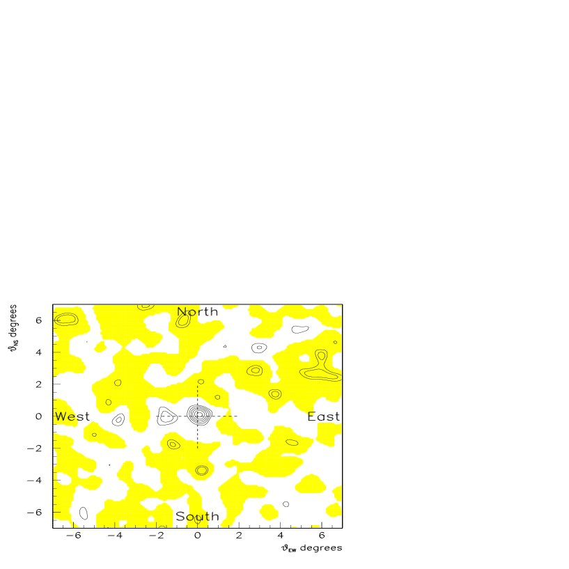
FIG. 4.: Contour map of normalised deviations, $Z$, for a $\pm 7^{\circ}\times\pm 7^{\circ}$ region centred on the moon made with a rebinning kernel with $\sigma_{k}=0.333^{\circ}$. The contour lines are spaced by $\Delta Z=0.5$ and shown only where $|Z|\geq 2.0$. Regions with $Z>0$ are shaded.

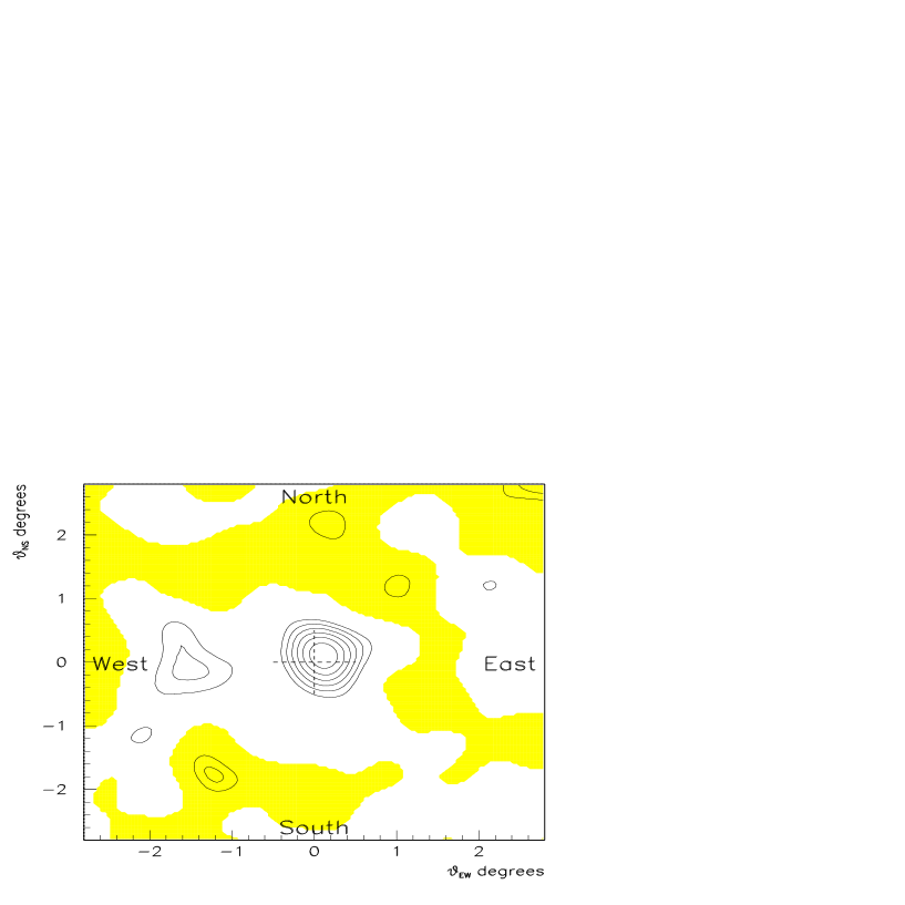
FIG. 5.: Contour map of normalised deviations, $Z$, for a $\pm 2.8^{\circ}\times\pm 2.8^{\circ}$ region centred on the moon made with a rebinning kernel with $\sigma_{k}=0.29^{\circ}$. The contour lines are spaced by $\Delta Z=0.5$ and shown only where $|Z|\geq 2.0$. Regions with $Z>0$ are shaded.

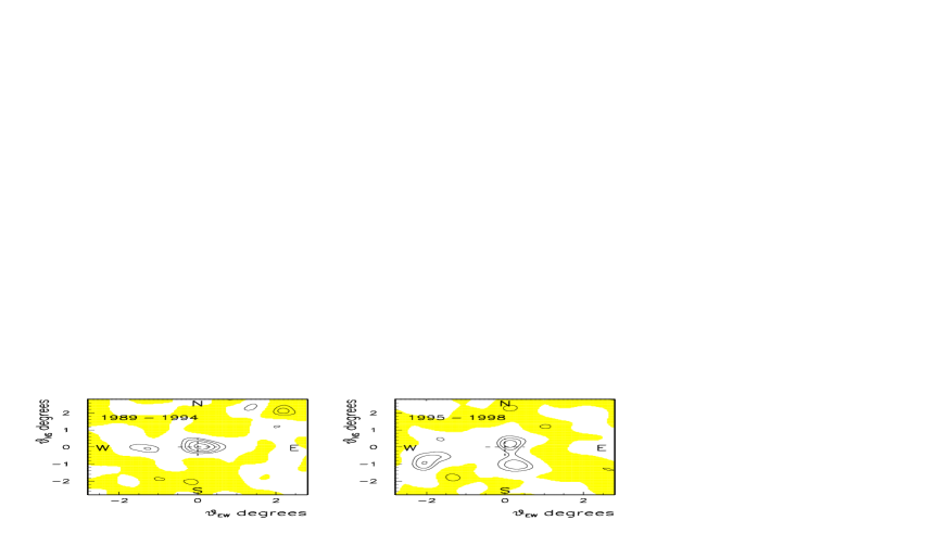
FIG. 6.: Contour maps of normalised deviations, $Z$, for a $\pm 2.8^{\circ}\times\pm 2.8^{\circ}$ region centred on the moon made with $\sigma_{k}=0.29^{\circ}$ for the periods 1989 – 1994 (left) and 1995 – 1998 (right). The contour lines are spaced by $\Delta Z=0.5$ and shown only where $|Z|\geq 2.0$. Regions with $Z>0$ are shaded.

REFERENCES

- [1] W. W. M. Allison et al., Nucl. Instr. and Meth. A 376, 377 (1996).
- [2] W. W. M. Allison et al., Nucl. Instr. and Meth. A 381, 385 (1996).
- [3] G. W. Clark, Phys. Rev. 108, 450 (1957).
- [4] J. Lloyd-Evans, Proceedings of the IXXth ICRC, La Jolla, California (1985).
- [5] D.E. Alexandreas et al., Phys. Rev. D43, 1735 (1991).
- [6] A. Borione et al., Phys. Rev. D49, 1171 (1994).
- [7] M. Merck et al., Astroparticle Phys. 5, 379 (1996).
- [8] M. Amenomori et al., Phys. Rev. D47, 2675 (1993).
- [9] M. Amenomori et al., Astrophys. J, 415, L147 (1994).
- [10] M. Amenomori et al., Astrophys. J, 464, 954 (1996).
- [11] S. Cecchini, for the Macro collaboration, Proceedings of the XXIVth ICRC, Vol. 1, pp 582 – 584, Rome (1995).
- [12] M. Ambrosio et al., Phys. Rev. D59, 012003 (1999).
- [13] W. W. M. Allison et al., in preparation.
- [14] M. A. Thomson, D. Phil Thesis, Oxford University (1991).
- [15] S.M. Kasahara et al., Phys. Rev. D55, No. 9, 5282 (1997).
- [16] C. Forti et al., Phys. Rev. D42, 3668 (1990).
- [17] R. S. Fletcher, T. K. Gaisser, P. Lipari and T. Stanev, Phys. Rev. D50, 5710 (1994)
- [18] P. Duffet-Smith, “Astronomy with your personal computer”, (Cambridge University Press, Cambridge), (1985).
- [19] D. Rabinowitz and D. Siegmund, Statistica Sinica, 7, No. 1, 167 (1997).
- [20] D. Siegmund and K. J. Worsley, Ann. Statist. 23, No. 2, 608 (1995).