In experiments with the CMD-2 detector at the VEPP-2M electron-positron collider at Novosibirsk about 150000 $e^{+}e^{-}\rightarrow\pi^{+}\pi^{-}$ events were recorded in the center-of-mass energy range from 0.61 up to 0.96 GeV. The result of the pion form factor measurement with a 1.4% systematic error is presented. The following values of the $\rho$-meson and $\rho-\omega$ interference parameters were found: $\mathrm{M}_{\rho}=(775.28\pm 0.61\pm 0.20)$ MeV, $\Gamma_{\rho}=(147.70\pm 1.29\pm 0.40)$ MeV, $\Gamma(\rho\rightarrow e^{+}e^{-})=(6.93\pm 0.11\pm 0.10)$ keV, $Br(\omega\rightarrow\pi^{+}\pi^{-})=(1.32\pm 0.23)\%$. © Budker Institute of Nuclear Physics

1 Introduction

The cross-section of the process $e^{+}e^{-}\rightarrow\pi^{+}\pi^{-}$ is given by

$$\sigma=\frac{\pi\alpha^{2}}{3s}\beta^{3}_{\pi}\left|F_{\pi}(s)\right|^{2},$$

where $F_{\pi}(s)$ is the pion form factor at the center-of-mass energy squared $s$ and $\beta_{\pi}$ is the pion velocity.

The pion form factor measurement is important for a number of physics problems. Detailed experimental data in the time-like region allows measurement of the parameters of the $\rho(770)$ meson and its radial excitations. Extrapolation of the energy dependence of the pion form factor to the point $s=0$ gives the value of the pion electromagnetic radius. Exact data on the pion form factor is necessary for precise determination of the ratio

$$R=\sigma(e^{+}e^{-}\rightarrow hadrons)/\sigma(e^{+}e^{-}\rightarrow\mu^{+}\mu^{-}).$$

Knowledge of R with high accuracy is required to evaluate the hadronic contribution $a_{\mu}^{had}$ to the anomalous magnetic moment of the muon $(g-2)_{\mu}$ [1]. About 87% of the hadronic contribution in this case comes from $s<2\;\mathrm{GeV^{2}/c^{2}}$ (VEPP-2M range), and about 72% — from $e^{+}e^{-}\rightarrow\pi^{+}\pi^{-}$ channel with $s<2\;\mathrm{GeV^{2}/c^{2}}$ [2, 3]. The E821 experiment at BNL [4] has collected its first data in 1997 and will ultimately measure $(g-2)_{\mu}$ with a 0.35 ppm accuracy. To calculate the hadronic contribution with the desired precision the systematic error in R should be below 0.5%. Therefore a new measurement of the pion form factor with a low systematic error is required.

Experiments at the VEPP-2M collider[5], which started in the early 70s, yielded a number of important results in $e^{+}e^{-}$ physics at low center-of-mass energies from 360 to 1400 MeV. The high precision measurement of the pion form factor at VEPP-2M was done in the late 70s – early 80s by OLYA and CMD groups [6]. In the CMD experiment, 24 points from 360 to 820 MeV were studied with a systematic uncertainty of about 2%. In the OLYA experiment, the energy range from 640 to 1400 MeV was scanned with small energy steps and the systematic uncertainty varied from 4% at the $\rho$-meson peak to 15% at 1400 MeV.

ID	Date	$2E$, GeV	Number of energy points	$N_{e^{+}e^{-}\rightarrow\pi^{+}\pi^{-}}$
1	Jan–Feb 1994	0.81–1.02	14	35000
2	Nov–Dec 1994	0.78–0.81	10	66000
3	Mar–Jun 1995	0.61–0.79	20	85000
4	Oct–Nov 1996	0.37–0.52	10	4500
5	Feb–Jun 1997	0.98–1.38	37	75000
6	Mar–Jun 1998	0.36–0.97	37	1900000

Table 1: CMD-2 runs dedicated to R measurement

During 1988-92 a new booster was installed to allow higher positron currents and injection of the electron and positron beams directly at the desired energy. During 1991-92 a new detector CMD-2 was installed at VEPP-2M, and in 1992 it started data taking. The pion form factor measurement was one of the major experiments planned at CMD-2. The energy scan of the whole VEPP-2M 0.36-1.38 GeV energy range was performed in six separate runs listed in Table 1. The energy range below the $\phi$ meson was scanned twice (in 94-96 and in 98).

In this article we present results of the analysis of the data from runs 1–3. The data were taken at 43 energy points with the center-of-mass energy from 0.61 GeV up to 0.96 GeV with a 0.01 GeV energy step. The small energy step allows calculation of hadronic contributions in model-independent way. In the narrow energy region near the $\omega$-meson the energy steps were $0.002\div 0.006$ GeV in order to study the $\omega$-meson parameters and the $\rho-\omega$ interference. Since the form factor is changing relatively fast in this energy region, it was important that the beam energy was measured with the help of the resonance depolarization technique at almost all energy points. That allowed a significant decrease of the systematic error coming from the energy uncertainty.

Figure 1: Detector CMD-2. 1 — beam pipe, 2 — drift chamber, 3 — Z-chamber, 4 — main solenoid, 5 — compensating solenoid, 6 — endcap (BGO) calorimeter, 7 — barrel (CsI) calorimeter, 8 — muon range system, 9 — magnet yoke, 10 — storage ring lenses

The CMD-2 (Fig. 1) is a general purpose detector consisting of the drift chamber, the proportional Z-chamber, the barrel (CsI) and the endcap (BGO) electromagnetic calorimeters and the muon range system. The drift chamber, Z-chamber and the endcap calorimeters are installed inside a thin superconducting solenoid with a field of 10 kGs. More details on the detector can be found elsewhere [7, 8, 9]. The data described here was taken before the endcap calorimeter was installed.

Two independent triggers were used during data taking. The first one, charged trigger, analyses information from the drift chamber and the Z-chamber and triggers the detector if at least one track was found. For 0.81–0.96 GeV energy points there was an additional requirement for the total energy deposition in the calorimeter to be greater than a 20–30 MeV threshold. The second one, neutral trigger, triggers the detector according to information from the calorimeter only. Events triggered by the charged trigger were used for analysis, while events triggered by the neutral trigger were used for trigger efficiency monitoring.

2 Data analysis

2.1 Selection of collinear events

Figure 2: Definition of parameters for two track events

The data was collected at 43 energy points. At the beam energy of 405 MeV the data was collected in two different runs with different detector and trigger conditions. Therefore, two independent results for this energy point are presented.

From more than $4\cdot 10^{7}$ triggers about $4\cdot 10^{5}$ were selected as collinear events. The selection criteria were as follows.

1. The event was triggered by the charged trigger. Other triggers may be present as well.

2. Only one vertex with two oppositely charged tracks was found in the drift chamber.

3. Distance from the vertex to the beam axis $\rho$ is less than 0.3 cm.

4. Z-coordinate of the vertex (distance to the interaction point along the beam axis) $|Z|$ is less than 8 cm.

5. Average momentum of two tracks $(p_{1}+p_{2})/2$ is between 200 and 600 MeV/c.

6. Acollinearity of two tracks in the plane transverse to the beam axis $|\Delta\varphi|=|\pi-|\varphi_{1}-\varphi_{2}||$ is less than 0.15 radians.

7. Acollinearity of two tracks in the plane that contains the beam axis $|\Delta\Theta|=|\Theta_{1}-(\pi-\Theta_{2})|$ is less than 0.25 radians.

8. Average polar angle of two tracks $[\Theta_{1}+(\pi-\Theta_{2})]/2$ is between $\Theta_{min}$ and $(\pi-\Theta_{min})$. All analysis was done separately for $\Theta_{min}=1.0$ and $\Theta_{min}=1.1$ radian.

Because of the unfortunate accident the high voltage was off for two neighbouring lines of the CsI calorimeter during the data taking in the 0.61–0.784 GeV energy region. In order to avoid additional calorimeter inefficiency, events with $4.35<\varphi_{+}<4.95$ or $3.90<\varphi_{-}<4.50$ have been removed from analysis for corresponding energy points (angles are measured in radians). Events with $1.05<\varphi_{+}<1.65$ or $0.55<\varphi_{-}<1.15$ were additionally removed for 0.65–0.70 GeV energy points.

Definition of the collinear event parameters, such as $\rho$, $\Theta_{1,2}$, $\varphi_{1,2}$, is illustrated in Fig. 2.

2.2 Event separation

2.2.1 Likelihood function

Figure 3: $E^{+}$ versus $E^{-}$ distribution for collinear events for 0.8 GeV energy point

The selected sample of events consists of collinear events $e^{+}e^{{}_{-}}\rightarrow e^{+}e^{-},$ $e^{+}e^{{}_{-}}\rightarrow\pi^{+}\pi^{-}$, $e^{+}e^{{}_{-}}\rightarrow\mu^{+}\mu^{{}_{-}}$ and background events mainly due to cosmic muons. The energy deposition in the barrel CsI calorimeter by negatively $(E^{-})$ and positively $(E^{+})$ charged particles were used for event separation. The distribution of $E^{+}$ versus $E^{-}$ is shown in Fig. 3. Electrons and positrons usually have large energy deposition since they produce electromagnetic showers. Muons usually have small energy deposition since they are minimum ionising particles. Pions can interact as minimum ionising particles producing small energy deposition or have nuclear interactions inside the calorimeter, resulting in long tails to a higher value of the energy deposition.

The separation was based on the minimization of the following unbinned likelihood function:

$$L=-\sum_{events}\ln\left(\sum_{a}N_{a}\cdot f_{a}(E^{+},E^{-})\right)+\sum_{a}N_{a},$$ (1)

where $a$ is the event type ($a=ee$, $\mu\mu$, $\pi\pi$, $cosmic$), $N_{a}$ is the number of events of the type $a$ and $f_{a}(E^{+},E^{-})$ is the probability density for a type $a$ event to have energy depositions $E^{+}$ and $E^{-}$. It was assumed that $E^{+}$ is uncorrelated with $E^{-}$ for events of the same type, so we can factorize the probability density:

$$f_{a}(E^{+},E^{-})=f_{a}^{+}(E^{+})\cdot f^{-}_{a}(E^{-}).$$

For $e^{+}e^{-}$, $\mu^{+}\mu^{-}$ pairs and cosmic events the energy deposition distribution is the same for negatively and positively charged particles, while these distributions are significantly different for $\pi^{+}$ and $\pi^{-}$. Therefore $f_{a}^{+}\equiv f^{-}_{a}$ for $a=ee,\;\mu\mu$ and $cosmic$, but for pions these functions are different. The probability density functions are described in detail in the following sections.

In minimization the ratio $N_{\mu\mu}/N_{ee}$ was fixed according to the QED calculation

$$\frac{N_{\mu\mu}}{N_{ee}}=\frac{\sigma_{\mu\mu}\cdot(1+\delta_{\mu\mu})\left(1+\alpha_{\mu\mu}\right)\varepsilon_{\mu\mu}}{\sigma_{ee}\cdot(1+\delta_{ee})\left(1+\alpha_{ee}\right)\varepsilon_{ee}},$$

where $\sigma$ is the Born cross-section, $\delta$ is a radiative correction, $\alpha$ is the correction for the experimental resolution of $\Theta$ angle measurement and $\varepsilon$ is the reconstruction efficiency (see sec. 2.3 for details). The likelihood function (1) was rewritten to have the following global fit parameters:

$$(N_{ee}+N_{\mu\mu}),\quad\frac{N_{\pi\pi}}{N_{ee}+N_{\mu\mu}},\quad N_{cosmic}$$

instead of $N_{ee}$, $N_{\mu\mu}$, $N_{\pi\pi}$ and $N_{cosmic}$. The number of cosmic events $N_{cosmic}$ was determined before the fit as described below, and was fixed during the fit.

2.2.2 Rejection of background events

Figure 4: To determination of number of cosmic background events

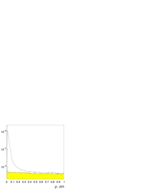
(a) $\rho$-distribution

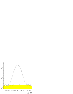
(b) $Z$-distribution

Figure 5: $\rho$- and $Z$-distributions for background and collinear events. Empty histograms correspond to all selected events, filled histograms correspond to background events only

Cosmic background events can be separated from the beam-produced collinear events by the distance $\rho$ from the vertex to beam axis and (or) by the $Z$-coordinate of the vertex. The $\rho$-distribution for collinear events has a narrow peak around 0, while the same distribution for the background events is almost flat (Fig. 5(a)). Similarly, the $Z$-distribution for collinear events is Gaussian like, while it is almost flat for the background events (Fig. 5(b)). Assuming that $\rho$- and $Z$-distributions for cosmic events are not correlated and that all events with $\rho>0.5$ cm or $|Z|>8$ cm are cosmic events, one can calculate the number of background events in the signal region from the number of events out of the signal region.

Let us define $N_{X}$ as the number of cosmic events in the signal region ($\rho<0.3$ cm, $|Z|\leq 8$ cm) and $N_{1,2,3}$ as the number of events in different out-of-signal $\rho-Z$ regions (see Fig. 4):

$$\left\{\begin{array}[]{l}N_{1}=N\bigm{|}_{\rho<0.3;\;8<|Z|<12}\\ N_{2}=N\bigm{|}_{0.5<\rho<1.0;\;|Z|\leq 8}\\ N_{3}=N\bigm{|}_{0.5<\rho<1.0;\;8<|Z|<12}\end{array}\right..$$

Then under assumptions mentioned above we can derive:

$$N_{X}=\frac{N_{2}}{N_{3}}\cdot N_{1}=\frac{N_{1}}{N_{3}}\cdot N_{2}.$$

$N_{X}$ is equal to $N_{cosmic}$ only statistically. The confidence interval for $N_{cosmic}$, corresponding to one standard deviation, is

$$N_{cosmic}\approx N_{X}\pm\sqrt{5N_{X}}.$$

In order to take that into account, the $N_{cosmic}$ value was fixed to the $N_{X}$ value during fit, but $\Delta N_{X}$ was added to $\Delta N_{\pi\pi}$ at the end.

2.2.3 Energy deposition parametrization

In order to construct the likelihood function (1) it is very convenient to have an analytical form for energy deposition distributions. We parametrize all energy depositions by the linear combination of two types of Gaussian-like functions, described below.

Normal distribution

$g(x;x_{0},\sigma)$

$$g(x;x_{0},\sigma)=\frac{1}{\sqrt{2\pi}\sigma}\exp\left[-(x-x_{0})^{2}/2\sigma^{2}\right],$$

where the parameters are the mean value $x_{0}$ and the standard deviation $\sigma$. The Gaussian is normalized at the $(-\infty,+\infty)$ interval, but energy deposition values belong to the $[0,+\infty)$ range. Therefore for parametrization the Gaussian normalized at the $[0,+\infty)$ range is used:

$$g(x;x_{0},\sigma)/\left[1-I\left(-\frac{x_{0}}{\sigma}\right)\right],$$

where

$$I(x)=\frac{1}{\sqrt{2\pi}}\int_{-\infty}^{x}\exp\left(-\frac{t^{2}}{2}\right)dt.$$

Normal logarithmic distribution[10]

$g_{l}(x;x_{0},\sigma,\eta)$

$$g_{l}(x;x_{0},\sigma,\eta)=\frac{1}{\sqrt{2\pi}\sigma}\cdot\frac{\eta}{\sigma_{0}}\cdot\exp\left\{-\frac{1}{2}\left[\frac{\ln^{2}\left(1-\frac{x-x_{0}}{\sigma}\eta\right)}{\sigma_{0}^{2}}+\sigma_{0}^{2}\right]\right\},$$

where

$$\sigma_{0}=\ln\left(\eta\sqrt{2\ln 2}+\sqrt{1+\eta^{2}\cdot 2\ln 2}\right)\left/\sqrt{2\ln 2}\right..$$

Parameters of this function are the most probable energy $x_{0}$, the $\sigma=\mathrm{FWHM}/2.35$ and the asymmetry $\eta$. If $\eta=0$, the logarithmic Gaussian is equal to the plain Gaussian:

$$g_{l}(x;x_{0,}\sigma,\eta)\left|{}_{\eta=0}\equiv g(x;x_{0},\sigma).\right.$$

The function is normalized at the $[-\infty,x_{0}+\sigma/\eta]$ interval:

$$\int_{-\infty}^{x_{0}+\sigma/\eta}g_{l}(x)dx=1,$$

but in our case its integral over the range $(-\infty,0]$ is negligible and it is assumed that this function is normalized at the $[0,x_{0}+\sigma/\eta]$ interval.

Since both functions are normalized, it is easy to construct the normalized energy deposition distribution.

2.2.4 Correction of energy deposition for polar angle

(a) Energy deposition versus $\Theta$ for collinear events before correction

(b) Average energy deposition versus $\Theta$ for electrons and cosmic background events before correction

(c) Energy deposition versus $\Theta$ for collinear events after correction

(d) Average energy deposition versus $\Theta$ for electrons and cosmic background events after correction

Figure 6: Correction of energy deposition for the polar angle of the track

Energy deposition in the calorimeter is correlated with the polar angle $\Theta$ of a track due to the dependence of calorimeter thickness on $\Theta$. So the probability density for an event of type $a$ to have energy deposition $E$ depends not only on $E$, but also on $\Theta$. In order to simplify the likelihood function, the energy deposition was corrected to make dependence of energy deposition on $\Theta$ negligible. In other words, instead of $f_{a}(E,\Theta)$ we are using $f_{a}(\overline{E})$, where $\overline{E}$ is the corrected energy deposition:

$$E\longrightarrow\overline{E}\quad to\;have\quad f_{a}(E,\Theta)\longrightarrow f_{a}(\overline{E}).$$

The correction procedure was performed as follows. First, two groups of events were selected: cosmic events and electrons. Selection criteria for both types of events are described below in sections 2.2.5 and 2.2.6. The scatter-plot of the energy deposition versus $\Theta$ for collinear events is shown in Fig. 6a. The full range of possible $\Theta$ values $\left[1,\pi-1\right]$ was divided into 50 equal bins and for each bin an average energy deposition was calculated for electrons and cosmic events.

The energy deposition of electrons depends on $\Theta$ because the CMD-2 calorimeter has only about $8X_{0}$ and therefore the shower leakage is not negligible. The effective calorimeter thickness increases for incident track angle away from normal. The corresponding small variation of the average energy deposition of electrons was fit to the parabolic function

$$E_{e}(\Theta)=E_{1}\cdot\left[1+\alpha(\Theta-\pi/2)^{2}\right],$$

where $E_{1}$ and $\alpha$ are the fit parameters.

Cosmic events contain minimum ionising particles and their energy deposition is proportional to the length in the calorimeter through which the particle passes. This length is proportional to $1/\sin\Theta$ , and the fit function in this case was

$$E_{c}(\Theta)=E_{0}/\sin\Theta,$$

where $E_{0}$ is a fit parameter. An example of the fit of the average energy depositions for electrons and cosmic tracks is shown in Fig. 6b.

The corrected energy was calculated as

$$\overline{E}(E,\Theta)=E\cdot\left[k_{c}(\Theta)+\frac{k_{e}(\Theta)-k_{c}(\Theta)}{E_{e}(\Theta)-E_{c}(\Theta)}\left(E-E_{c}(\Theta)\right)\right],$$

where $k_{c}(\Theta)=E_{0}/E_{c}(\Theta)$, $k_{e}(\Theta)=E_{1}/E_{e}(\Theta)$, $E_{c}(\Theta)$ and $E_{e}(\Theta)$ are the measured average energy deposition for cosmic and Bhabha events respectively. After such a correction the average energy deposition for both cosmic and Bhabha events does not depend on $\Theta$. In fact, if $E=E_{e}(\Theta)$, then $\overline{E}=E_{1}$; if $E=E_{c}(\Theta)$, then $\overline{E}=E_{0}$.

Since the energy deposition of cosmic events does not depend on the beam energy, the variations of $E_{0}$ reflects residual variations in the calibration of the CsI calorimeter. To correct for these variations, the energy deposition was normalized to have the average energy deposition of the cosmic events equal to 85 MeV (the arbitrary constant close to the experimental value) for all beam energies:

$$\overline{E}\longrightarrow\overline{E}\cdot\frac{85}{E_{0}}.$$

The scatter-plot of the corrected energy deposition versus $\Theta$ for collinear events is shown in Fig. 6c. The average energy deposition for electrons and cosmic events versus $\Theta$ after the correction is shown in Fig. 6d.

The described energy deposition correction was calculated independently for each energy point. In the all following sections $E$ actually means the corrected energy $\overline{E}$.

2.2.5 Energy deposition of cosmic events

As mentioned above, it is possible to select a pure sample of background events from the real data. In this case the selection criteria are the same as standard cuts for the collinear events, except that the distance $\rho$ from the vertex to the beam axis should be from 5 to 10 mm (instead of less than 3 mm). In order to make the selected sample of background events even cleaner, the fact that there are two clusters in the event was used. Analysing the energy deposition of one cluster, the energy deposition of the other one was required to be less than 150 MeV. Since the clusters are independent, the strict limit on one cluster energy does not affect the energy deposition distribution for the other cluster.

The data for all energy points was combined together and the energy deposition of cosmic events was parametrized using the following function:

$$f(E)=p\cdot g_{l}(E;E_{0},\sigma,\eta)+(1-p)\cdot g_{l}(E;E_{0}+\alpha\sigma,\beta\sigma,\gamma\eta).$$ (2)

The fit result is presented in Fig. 7. The obtained function was used as the energy deposition for background events:

$$\begin{array}[]{c}f^{+}_{cosmic}(E)\equiv f^{-}_{cosmic}(E)\equiv f_{cosmic}(E),\vphantom{\Big{/}}\\ \lx@intercol f_{cosmic}(E)=0.69\cdot g_{l}(E;81.2,9.0,-0.175)+\vphantom{\Big{/}}\hfil\lx@intercol\\ \lx@intercol\hfil\qquad\qquad\qquad\qquad\qquad\qquad+0.31\cdot g_{l}(E;91.7,22.8,-0.186).\vphantom{\Big{/}}\lx@intercol\end{array}$$ (3)

In order to check the stability of the energy deposition for cosmic events, all energy points were combined into 4 groups: 0.61–0.70 GeV, 0.71–0.778 GeV, 0.780–0.810 GeV and 0.810–0.960 GeV. The energy deposition of the selected background events for each group was fitted with the function (3). Results of the fit are demonstrated in Fig. 8.

Figure 7: Fit of the energy deposition for cosmic events with the function (2). Fit parameters: P1 – number of events, P2 – $p$, P3 – $E_{0}$, P4 – $\sigma$, P5 – $\eta$, P6 – $\alpha$, P7 – $\beta$, P8 – $\gamma$

(a) Group 0.61–0.70 GeV

(b) Group 0.71–0.778 GeV

(c) Group 0.780–0.810 GeV

(d) Group 0.810–0.960 GeV

Figure 8: Fit of energy deposition of cosmic events with the function (3). Data is combined into 4 groups of energy points. Fit parameter: P1 – number of events

The probability to have no cluster in the calorimeter (zero energy deposition) for cosmic event tracks was also measured and found to be negligible — less than 0.1%.

2.2.6 Energy deposition of electrons and positrons

(a) Fit of the positron energy deposition

(b) Fit of the electron energy deposition

Figure 9: Fit of the energy deposition of electrons and positrons at center-of-mass energy 0.9 GeV. Fit parameters: P1 – $p_{w}$, P2 – $E_{0}$, P3 – $\sigma$, P4 – $\eta$, P5 – number of events, P6 – $\alpha$, P7 – $\beta$, P8 – $\gamma$

The energy deposition for electrons and positrons was obtained from the data. Electrons and positrons can be separated from mesons by their relatively high energy deposition in the calorimeter. If we have one “clean” electron (positron) in the event (a particle with a proper momentum and high energy deposition), then we know that the second particle is a positron (electron), and therefore may be used for the energy deposition study.

The test $e^{+}e^{-}\rightarrow e^{+}e^{-}$ events were selected for the energy deposition study with the same selection criteria as for collinear events except for the following.

1. The distance $\rho$ from the vertex to the beam axis is less than 0.15 cm (instead of 0.3 cm).

2. The average momentum of the particles is within the 10 MeV/c range around the beam energy. This requirement allows to decrease significantly a small admixture of $e^{+}e^{-}\rightarrow\pi^{+}\pi^{-}$ events.

Analysing the energy deposition in one cluster, the energy deposition in the other one is required to be between $0.92E_{B}-100$ MeV and $0.92E_{B}$, where $E_{B}$ is the beam energy. As for cosmic rays since the clusters are independent, the strict limit on one cluster energy does not affect the energy deposition distribution for the other cluster.

For each energy point the energy depositions of the selected electrons and positrons were fitted with the following function:

$$f(E)=(1-p_{w})\cdot g_{l}(E;E_{0},\sigma,\eta)+p_{w}\cdot g_{l}(E;E_{0}+\alpha\sigma,\beta\sigma,\gamma\eta).$$

After analysis of the fit results the following values of the parameters were found:

$$\alpha=-0.8,\quad\beta=3.0,\quad\gamma=1.4.$$

Again, as for cosmic rays, the probability to have no cluster was found to be negligible (less than 0.1%) for all energy points. Finally, the energy deposition of electrons and positrons was parametrized as:

$$\begin{array}[]{c}f^{+}_{ee}(E)\equiv f^{-}_{ee}(E)\equiv f_{ee}(E),\\ \\ f_{ee}(E)=(1-p_{w})\cdot g_{l}(E;E_{0},\sigma,\eta)+p_{w}\cdot g_{l}(E;E_{0}-0.8\sigma,3\sigma,1.4\eta),\end{array}$$ (4)

where $p_{w}$, $E_{0}$, $\sigma$ and $\eta$ are free parameters of the fit. An example of the electron and positron energy depositions is shown in Fig. 9.

2.2.7 Energy deposition of muons

(a) Energy deposition of 375 MeV muons

(b) Energy dependence of $E_{0}$

(c) Energy dependence of $\sigma_{0}$

Figure 10: Simulated energy deposition of muons

In the center-of-mass energy range above 0.6 GeV, muons produced in the reaction $e^{+}e^{-}\rightarrow\mu^{+}\mu^{-}$ interact with the calorimeter as the minimum ionising particles, and therefore their energy deposition can be obtained from the detector simulation. The simulation of the $e^{+}e^{-}\rightarrow\mu^{+}\mu^{-}$ events was performed for center-of-mass energies 0.6, 0.62, 0.64, 0.66, 0.68, 0.70, 0.74, 0.75, 0.76, 0.77, 0.78, 0.79, 0.80, 0.82, 0.85, 0.90, 0.95, 1.0 GeV. 10000 events were simulated for each energy point. Simulated events were processed by the standard offline reconstruction program and the standard selection criteria for collinear events were applied. Then the energy deposition of the simulated muons was corrected as described in sec. 2.2.4.

The resulting energy deposition for each energy point was parametrized by the following function:

$$f^{\mu}_{SIM}(E)=p_{1}\cdot\left[\,p_{2}\cdot g_{l}(E;E_{0},\sigma_{0},\eta)+\right.$$

$$\left.+(1-p_{2})\cdot g_{l}(E;E_{0},\beta\sigma_{0},\gamma\eta)\right]+(1-p_{1})\cdot g(E;E_{1},\sigma_{1}),$$

where $p_{1}$, $p_{2}$, $E_{0}$, $\sigma_{0}$, $E_{1}$, $\sigma_{1}$, $\eta$, $\beta$ and $\gamma$ are the free fit parameters.

In the simulation we have a perfectly calibrated calorimeter while the real data have an additional spread due to the uncertainty of the calibration coefficients. As a result, the real energy distribution is wider than that in the simulation. It could also be slightly shifted. To take that into account, the energy deposition distribution obtained from the simulation was modified to reflect the energy deposition of real muons:

$$\begin{array}[]{c}f_{\mu}^{+}(E)\equiv f_{\mu}^{-}(E)\equiv f_{\mu}(E),\vphantom{\Big{/}}\\ f_{\mu}(E)=f^{\mu}_{MIP}(E;k,\sigma_{x}),\vphantom{\bigg{/}}\\ \lx@intercol f^{\mu}_{MIP}(E;k,\sigma_{x})=p_{1}\cdot\left[\,p_{2}\cdot g_{l}(\tilde{E};E_{0},\tilde{\sigma}_{0},\eta)+\right.\vphantom{\bigg{/}}\hfil\lx@intercol\\ \lx@intercol\hfil\qquad\qquad\qquad\left.+(1-p_{2})\cdot g_{l}(\tilde{E};E_{0},\beta\tilde{\sigma}_{0},\gamma\eta)\right]+(1-p_{1})\cdot g(\tilde{E};E_{1},\tilde{\sigma_{1}}),\vphantom{\bigg{/}}\lx@intercol\\ \tilde{E}=E/k,\quad\tilde{\sigma}_{0}=\sqrt{\sigma_{0}^{2}+\sigma_{x}^{2}},\quad\tilde{\sigma}_{1}=\sqrt{\sigma_{1}^{2}+\sigma_{x}^{2}}.\vphantom{\Big{/}}\end{array}$$

The values of $p_{1}$, $p_{2}$, $E_{0}$, $\sigma_{0}$, $E_{1}$, $\sigma_{1}$, $\eta$, $\beta$ and $\gamma$ are fixed according to the simulation, so this function has only two free parameters: $k$ is the scale coefficient and $\sigma_{x}$ is the additional energy spread.

An example of the fit for one energy point as well as the energy dependence of $E_{0}$ and $\sigma_{0}$ parameters are shown in Fig. 10. The $k$ and $\sigma_{x}$ parameters for all energy points are shown in Fig. 15a and 15b respectively.

2.2.8 Energy deposition of pions

Pions produced in the reaction $e^{+}e^{-}\rightarrow\pi^{+}\pi^{-}$ may interact with the calorimeter in two ways: as minimum ionising particles or through nuclear interaction.

(a) Energy deposition of 400 MeV pions

(b) Energy dependence of $E_{0}$

(c) Energy dependence of $\sigma_{0}$

Figure 11: Simulated energy deposition of minimum ionising pions

The energy deposition of the minimum ionising pions was obtained from the detector simulation in the same way as for muons. The simulation was performed for the center-of-mass energies 0.6, 0.62, 0.64, 0.66, 0.68, 0.70, 0.75, 0.80, 0.85, 0.90, 0.95, 1.0 GeV. 10000 events were simulated for each energy point. Simulated events were processed by the standard offline reconstruction program and the standard selection criteria for collinear events were applied. Then the energy deposition of the simulated pions was corrected as described in sec. 2.2.4.

The resulting energy deposition for each energy point was parametrized by the same function as for muons:

$$f^{\pi}_{SIM}(E)=p_{1}\cdot\left[\,p_{2}\cdot g_{l}(E;E_{0},\sigma_{0},\eta)+\right.$$

$$\left.+(1-p_{2})\cdot g_{l}(E;E_{0},\beta\sigma_{0},\gamma\eta)\right]+(1-p_{1})\cdot g(E;E_{1},\sigma_{1}),$$

where $p_{1}$, $p_{2}$, $E_{0}$, $\sigma_{0}$, $E_{1}$, $\sigma_{1}$, $\eta$, $\beta$ and $\gamma$ are the free fit parameters depending on the beam energy. This function describes well the energy deposition only for those pions that do not stop in the calorimeter.

As was done for muons, the modified simulated energy deposition was used for the parametrization of the energy deposition of real pions:

$$\begin{array}[]{c}\lx@intercol f^{\pi}_{MIP}(E;k,\sigma_{x})=p_{1}\cdot\left[\,p_{2}\cdot g_{l}(\tilde{E};E_{0},\tilde{\sigma}_{0},\eta)+\right.\vphantom{\bigg{/}}\hfil\lx@intercol\\ \lx@intercol\hfil\qquad\qquad\qquad\left.+(1-p_{2})\cdot g_{l}(\tilde{E};E_{0},\beta\tilde{\sigma}_{0},\gamma\eta)\right]+(1-p_{1})\cdot g(\tilde{E};E_{1},\tilde{\sigma_{1}}),\vphantom{\bigg{/}}\lx@intercol\\ \tilde{E}=E/k,\quad\tilde{\sigma}_{0}=\sqrt{\sigma_{0}^{2}+\sigma_{x}^{2}},\quad\tilde{\sigma}_{1}=\sqrt{\sigma_{1}^{2}+\sigma_{x}^{2}}.\vphantom{\Big{/}}\end{array}$$

The values of $p_{1}$, $p_{2}$, $E_{0}$, $\sigma_{0}$, $E_{1}$, $\sigma_{1}$, $\eta$, $\beta$ and $\gamma$ were fixed according to the simulation, so this function has only two free parameters: the scale coefficient $k$ and the additional energy spread $\sigma_{x}$.

An example of the energy deposition of minimum ionising pions and the energy dependence of $E_{0}$ and $\sigma_{0}$ parameters are shown in Fig. 11. The $k$ and $\sigma_{x}$ parameters for all energy points are shown in Fig. 15a and 15b respectively.

The energy deposition of the nuclear interacted pions cannot be simulated well. Therefore, in this case we have chosen to use an empirical parametrization, which fits experimental data well:

$$f^{\pi}_{NI}(E;\sigma,p_{1\ldots N})=\frac{g(E;0,\sigma)+\sum\limits_{i=1}^{N}g(E;\frac{E_{0}}{N+1}i,\sigma)\cdot p_{i}^{2}}{1+\sum\limits_{i=1}^{N}p_{i}^{2}},$$

where $E_{0}$ is the beam energy, N is the number of Gaussian and $\sigma$ and $p_{1\ldots N}$ are the free fit parameters. All Gaussian are normalized at the $[0,+\infty]$, therefore $f^{\pi}_{NI}$ is also normalized. This function appears as a set of equidistant Gaussians of the same width but different area. The parametrization with $N=5$ or $6$ describes well the experimental data.

The energy depositions of the minimum ionising $\pi^{+}$ and $\pi^{-}$ are the same while they are quite different for nuclear interacted $\pi^{+}$ and $\pi^{-}$. Unlike electrons and muons, pions have a significant probability to have no cluster in the calorimeter and this probability is different for $\pi^{+}$ and $\pi^{-}$. According to this, the overall pion energy deposition was parametrized with the following functions:

$$f_{\pi}^{+}(E)=p_{0}^{+}\cdot\delta(E)+(1-p_{0}^{+})\times$$

$$\times\left[\,p^{+}_{MIP}\cdot f^{\pi}_{MIP}(E;k,\sigma_{x})+(1-p^{+}_{MIP})\cdot f^{\pi}_{NI}(E;\sigma^{+},p^{+}_{1\ldots N})\right],\vphantom{\bigg{/}}$$

$$f_{\pi}^{-}(E)=p_{0}^{-}\cdot\delta(E)+(1-p_{0}^{-})\times$$

$$\times\left[\,p^{-}_{MIP}\cdot f^{\pi}_{MIP}(E;k,\sigma_{x})+(1-p^{-}_{MIP})\cdot f^{\pi}_{NI}(E;\sigma^{-},p^{-}_{1\ldots N})\right],\vphantom{\bigg{/}}$$

where $p_{0}^{\pm}$, $p_{MIP}^{\pm}$, $k$, $\sigma_{x}$, $\sigma^{\pm}$, $p^{\pm}_{1\ldots N}$ are free fit parameters.

Pions produced in the $\phi(1020)$ decay to $3\pi$ were used to test whether the functions (2.2.8) and (2.2.8) describe the energy deposition of the real pions well enough. The CMD-2 has collected about 20 pb^-1 in the $\varphi$-meson energy range. About 100000 “clean” $\pi^{+}$ and $\pi^{-}$ were selected from the completely reconstructed $\varphi\rightarrow\pi^{+}\pi^{-}\pi^{0}$ events. The energy deposition of $\pi^{+}$ ($\pi^{-}$) with energies $345<E_{\pi}<355$ MeV and $425<E_{\pi}<435$ MeV together with the fit are shown in Fig. 12a and 12c (12b and 12d).

(a) $\pi^{+}$, $345<E_{\pi}<355$ MeV

(b) $\pi^{-}$, $345<E_{\pi}<355$ MeV

(c) $\pi^{+}$, $425<E_{\pi}<435$ MeV

(d) $\pi^{-}$, $425<E_{\pi}<435$ MeV

Figure 12: An example of the experimental energy deposition for pions of different energy. Pions were extracted from $\varphi\rightarrow\pi^{+}\pi^{-}\pi^{0}$ data. The energy depositions of $\pi^{+}$ and $\pi^{-}$ were fitted with functions (2.2.8) and (2.2.8) respectively

2.2.9 Fit results

The minimization of the likelihood function (1) was carried out for all energy points with the typical number of 10000 events per energy point with the following 27 free fit parameters:

• global parameters

  $$(N_{ee}+N_{\mu\mu}),\quad\frac{N_{\pi\pi}}{N_{ee}+N_{\mu\mu}}$$

• Electron energy deposition parameters

  $$p_{W},\quad E_{0},\quad\sigma,\quad\eta$$

• Muon energy deposition parameters

  $$k_{MIP},\quad\sigma_{x}^{\mu}$$

• Pion energy deposition parameters

  $$\sigma_{x}^{\pi},\quad p_{0}^{+},\quad p_{0}^{-},\quad p_{MIP}^{+},\quad p_{MIP}^{-},$$

  $$\sigma_{NI}^{+},\quad\sigma_{NI}^{-},\quad p^{+}_{1\ldots N},\quad p^{-}_{1\ldots N},\quad N=6$$

The number of background events was fixed during the fit. The scale parameter for minimum ionising muons and pions was the same (listed about as $k_{MIP}$).

The results of the minimization are shown in Fig. 13–15: the global parameters are shown in Fig. 13, the electron energy deposition parameters are shown in Fig. 14 and the muon and pion energy deposition parameters are shown in Fig. 15.

(a) $N_{ee}+N_{\mu\mu}$

(b) $N_{\pi\pi}/(N_{ee}+N_{\mu\mu})$

Figure 13: Results of the minimization of the likelihood function (1). The energy dependences of the global parameters are shown

(a) $E_{0}$

(b) $\sigma$

(c) $p_{W}$

(d) $\eta$

Figure 14: Results of the minimization of the likelihood function (1). The electron energy deposition parameters are shown

(a) $k_{MIP}$

(b) $\sigma_{x}^{\mu}$ and $\sigma_{x}^{\pi}$

(c) $p_{0}^{+}$ and $p_{0}^{-}$

(d) $p_{MIP}^{+}$ and $p_{MIP}^{-}$

Figure 15: Results of the minimization of the likelihood function (1). The muon and pion energy deposition parameters are shown

2.3 Form factor calculation

After the minimization of the likelihood function, the pion form factor was calculated as:

$$\left|F_{\pi}\right|^{2}=\frac{N_{\pi\pi}}{N_{ee}+N_{\mu\mu}}\times$$

$$\times\frac{\sigma^{B}_{ee}\cdot\left(1+\delta_{ee}\right)\left(1+\alpha_{ee}\right)\varepsilon_{ee}+\sigma^{B}_{\mu\mu}\cdot\left(1+\delta_{\mu\mu}\right)\left(1+\alpha_{\mu\mu}\right)\varepsilon_{\mu\mu}}{\sigma^{B}_{\pi\pi}\cdot\left(1+\delta_{\pi\pi}\right)\left(1+\alpha_{\pi\pi}\right)\left(1-\Delta_{H}\right)\left(1-\Delta_{D}\right)\varepsilon_{\pi\pi}}-$$

$$-\Delta_{3\pi},$$

where $N_{\pi\pi}/(N_{ee}+N_{\mu\mu})$ was obtained as a result of minimization, $\sigma^{B}_{a}$ are the Born cross-sections, $\delta_{a}$ are the radiative corrections, $\varepsilon_{a}$ are the efficiencies, including trigger and reconstruction efficiencies, $\alpha_{a}$ are the corrections for the experimental resolution of the $\Theta$ angle measurement, $\Delta_{H}$ is the correction for pion losses due to nuclear interactions, $\Delta_{D}$ is the correction for pion losses due to decays in flight and $\Delta_{3\pi}$ is the correction for the misidentification of $\pi^{+}\pi^{-}\pi^{0}$ events as a $\pi^{+}\pi^{-}$ pair.

Together with the pion form factor, the cross-section of $e^{+}e^{-}$ annihilation to $\pi^{+}\pi^{-}$ was calculated as

$$\sigma_{\pi\pi}=\frac{\pi\alpha^{2}}{3s}\left(1-\frac{4m_{\pi}^{2}}{s}\right)^{3/2}\cdot\left|F_{\pi}\right|^{2},$$

and the luminosity integral as

$$\int Ldt=\frac{N_{ee}+N_{\mu\mu}}{\sigma_{ee}^{B}\cdot(1+\delta_{ee})(1+\alpha_{ee})\varepsilon_{ee}+\sigma_{\mu\mu}^{B}\cdot(1+\delta_{\mu\mu})(1+\alpha_{\mu\mu})\varepsilon_{\mu\mu}}.$$

2.3.1 Radiative corrections

Figure 16: Radiative corrections for $e^{+}e^{-}\rightarrow e^{+}e^{-},\pi^{+}\pi^{-},\mu^{+}\mu^{-}$ events

The radiative corrections are shown in Fig. 16. The calculation of the radiative corrections for $e^{+}e^{-}\rightarrow e^{+}e^{-}$ events was based on [11]. The estimated systematic error is $\sim 1\%$. Radiative corrections for $e^{+}e^{-}\rightarrow\mu^{+}\mu^{-},\pi^{+}\pi^{-}$ were calculated according to [12] and [13]. The estimated systematic error is $0.2-0.5\%$. The contribution from the lepton and hadron vacuum polarization is included in the radiative corrections for $e^{+}e^{-}\rightarrow e^{+}e^{-},\mu^{+}\mu^{-}$, but excluded from the radiative correction for $e^{+}e^{-}\rightarrow\pi^{+}\pi^{-}$. Some details about the radiative correction calculation could be found in [9].

The radiative correction for $e^{+}e^{-}\rightarrow\pi^{+}\pi^{-}$ depends on the energy behaviour of the $e^{+}e^{-}\rightarrow\pi^{+}\pi^{-}$ cross-section itself. In order to take that into account, the calculation of this correction was done via a few iterations. At the first iteration, the existing $\left|F_{\pi}(s)\right|^{2}$ data were used for the calculation of the radiative correction. Using the calculated correction, we obtain $\left|F_{\pi}(s)\right|^{2}$. At subsequent iterations, $\left|F_{\pi}(s)\right|^{2}$ data obtained from the previous step, were used. It was found that after 3 iterations $\left|F_{\pi}(s)\right|^{2}$ values become stable.

2.3.2 Trigger efficiency

The trackfinder (TF) signal, neutral trigger (NT) signal and the calorimeter “OR” (CSI) trigger signal have been used for detector triggering during 1994-1995 runs. The trackfinder uses only the drift chamber and the Z-chamber data for a fast decision whether there is at least one track in the event. The neutral trigger analyses the geometry and energy deposition of the fired calorimeter rows. The calorimeter “OR” signal appears when there is at least one triggered calorimeter row.

Two different trigger settings have been used during 1994-1995 runs. For 810(2)-960 MeV energy points the trigger was “(TF.and.CSI).or.NT” while for other energy points the trigger was “TF.or.NT”. For analysis we use only those events where the trackfinder has found the track. If the trackfinder efficiency is $\varepsilon_{TF}$ and the CSI signal efficiency is $\varepsilon_{CSI}$, the overall trigger efficiency is $\varepsilon_{TF}\cdot\varepsilon_{CSI}$ for 810(2)-960 MeV energy points and $\varepsilon_{TF}$ for 610-810(1) MeV energy points.

For the measurement of the trackfinder efficiency $e^{+}e^{-}\rightarrow e^{+}e^{-}$ events have been selected using only the calorimeter data (see the next section for details). Additionally, the positive decision of the neutral trigger was required. Analysing the probability to have also a positive decision of the trackfinder, its efficiency for $e^{+}e^{-}\rightarrow e^{+}e^{-}$ events can be calculated. The result is shown in Fig. 17(a). All types of collinear events are similar from the trackfinder point of view — they have two collinear tracks and the track momenta are very close for different types of events. It is seen from the picture that the TF efficiency is high enough and that there is no visible energy dependence of the efficiency. Therefore we assume that the trackfinder efficiency is the same for all types of collinear events and hence cancels in (2.3).

For the measurement of the CSI signal efficiency the fact that there are two clusters in the collinear event have been used: the CSI efficiency for a single cluster has been measured and was used for the calculation of the CSI efficiency for the event. The collinear events have been selected using the standard cuts. Then, the probability to trigger the CSI signal was measured for one cluster as a function of its energy. Using the measured probability and our knowledge about the energy deposition of particles of different types, the efficiency to trigger the CSI signal was calculated for different types of events. Results for 810(2)-960 MeV energy points are shown in Fig. 17(b). For simplicity, the values of 99.5% for pions and 99.2% for muons for the CSI efficiency were used for all 810-960 MeV energy points.

(a) Trackfinder efficiency for $e^{+}e^{-}\rightarrow e^{+}e^{-}$ events

(b) CSI signal efficiency for collinear events

Figure 17: Trigger efficiency for collinear events

2.3.3 Reconstruction efficiency

Figure 18: Reconstruction efficiency for all energy points

The reconstruction efficiency was measured for $e^{+}e^{-}\rightarrow e^{+}e^{-}$ events using the experimental data: events were selected using only the calorimeter data, and then the probability to reconstruct two collinear tracks was measured. Since the selection criteria for collinear events are based on tracking data only, the measured probability is the reconstruction efficiency.

The following selection criteria based only on the calorimeter data, were used.

1. There are exactly two clusters in the calorimeter.

2. There is a hit in the Z-chamber near each cluster. This requirement selects the clusters produced by the charged particle.

3. The energy deposition of both clusters is between $(0.82\cdot E_{B}-40)$ and $(0.82\cdot E_{B}+50)$ MeV. This is typical for $e^{+}$ and $e^{-}$, but not for other particles.

4. The clusters are collinear if one takes into account the particle motion in the detector magnetic field:

   $$|\pi-(\Theta_{1}+\Theta_{2})|<0.1,$$

   $$\left|\left|\pi-|\varphi_{1}-\varphi_{2}|\right|-2\arcsin\left(\frac{R\cdot 0.3B}{2\cdot E_{B}\cdot\sin\Theta}\right)\right|<0.1,$$

   where $\Theta$ and $\varphi$ are the polar and azimuthal angles of the cluster, $R$ is the effective calorimeter radius (45 cm) and $B$ is the magnetic field (typically 10 kGs).

5. The event was triggered by the trackfinder. Other triggers may be present.

The selected sample contain only $e^{+}e^{-}\rightarrow e^{+}e^{-}$ events with negligible ($<0.5\%$) background. If the number of selected events is $N_{0}$ and the number of events, which in addition satisfy the standard selection criteria for collinear events is $N_{1}$, then the reconstruction efficiency is

$$\varepsilon_{rec}={N_{1}}/{N_{0}}.$$

The measured reconstruction efficiency is shown in Fig. 18 (filled dots). The efficiency drops down for beam energies below 400 MeV. This additional inefficiency is completely explained by the lower precision of the $\Theta$ angle measurement for these energy points. The empty dots in the same plot represent the reconstruction efficiency for the same selection criteria for collinear events except for $\Delta\Theta$.

As in studying the trigger efficiency, all types of collinear events are very similar from the point of view of the tracking reconstruction code. Therefore we assume that the reconstruction efficiency is the same for all types of collinear events and hence it cancels in (2.3).

2.3.4 Correction for the limited accuracy of the polar angle measurement

There is a special type of correction that arises since there is finite experimental resolution in the measurement of the $\Theta$ angles of tracks. Since we require the measured, rather than real, $\;\Theta_{avr}=[\Theta_{1}+(\pi-\Theta_{2})]/2\;$ to be within $[\Theta_{min},\pi-\Theta_{min}]$ interval, the visible cross-section is slightly different from

$$\int_{\Theta_{min}}^{\pi-\Theta_{min}}\frac{d\sigma}{d\Omega}\cdot 2\pi\sin\Theta\,d\Theta.$$

The corresponding correction, denoted $\alpha$ in (2.3), was calculated as

$$1+\alpha=\int\limits_{\Theta_{min}}^{\pi-\Theta_{min}}d\Theta\int\limits_{0}^{\pi}d\Theta^{\prime}\cdot f(\Theta^{\prime})p(\Theta^{\prime},\Theta)\left/\int\limits_{\Theta_{min}}^{\pi-\Theta_{min}}d\Theta\cdot f(\Theta)\right.,$$

where $f(\Theta)$ is the theoretical $\Theta$-distribution and $p(\Theta^{\prime},\Theta)$ is the detector response function taken as

$$p(\Theta^{\prime},\Theta)=\frac{1}{\sqrt{2\pi}\sigma_{\Theta}}\exp\left[-\frac{(\Theta^{\prime}-\Theta)^{2}}{2\sigma_{\Theta}^{2}}\right]$$

where $\sigma_{\Theta}$ is the experimental resolution of $\Theta_{avr}$ measurement. The resolution and the corresponding corrections for different types of collinear events for all energy points are shown in Fig. 19.

(a) $\Theta$-resolution

(b) Correction to cross-section

Figure 19: The experimental resolution of the average polar angle measurement and the corresponding correction to cross-sections

2.3.5 Correction for pion losses due to nuclear interactions

Figure 20: The probability $\Delta_{H}$ to lose the $e^{+}e^{-}\rightarrow\pi^{+}\pi^{-}$ event from the sample of collinear events due to nuclear interactions of pions with the beam pipe or drift chamber inner support

Unlike electrons and muons, a small fraction of pions has nuclear interactions in the beam pipe and therefore is lost from the selected samples of collinear events. The corresponding correction was calculated under the assumption that the event is lost from the collinear event sample if at least one pion had an inelastic nuclear interaction in the beam pipe or drift chamber inner support. The calculations were done separately for cross-sections obtained from two packages available in GEANT[14] for simulation of nuclear interactions — FLUKA[15] and GHEISHA[16]. The resulting correction is shown in Fig. 20. It has been shown [17] that FLUKA is more successful in describing experimental data about nuclear interactions of pions in our energy range, and therefore the results obtained from FLUKA were used for the cross-section correction while the difference between two calculations was added to the systematic error.

2.3.6 Correction for pion losses due to decays in flight

Figure 21: The probability $\Delta_{D}$ to lose the $e^{+}e^{-}\rightarrow\pi^{+}\pi^{-}$ event from the sample of collinear events due to pion decay in flight

A small fraction of pions decays in flight inside the drift chamber and the corresponding event may not be recognized as collinear if the decay angle between the pion and secondary muon is large enough. Depending on the beam energy 2-4% of the $e^{+}e^{-}\rightarrow\pi^{+}\pi^{-}$ events have a decayed pion. But the maximum decay angle for the analysed energy range is small — 80-150 mrad depending on the pion energy — and therefore more than 90% of such events are reconstructed as a pion pair. The probability to lose a pion pair due to the pion decay in flight was found from simulation and is shown in Fig. 21.

2.3.7 Correction for the background from $\omega\rightarrow 3\pi$

Figure 22: The $\Delta_{3\pi}$ contribution to the pion form factor from $\omega\rightarrow 3\pi$

There is a small probability to identify the $\pi^{+}\pi^{-}\pi^{0}$ final state as a $\pi^{+}\pi^{-}$ pair. Therefore the measured pion form factor is slightly bigger than it should be. This effect is significant only in the narrow energy range near the $\omega$-meson. The corresponding probability was estimated from simulation and was found to be $5\cdot 10^{-3}$ for $\Theta_{min}=1.0$ and $4\cdot 10^{-3}$ for $\Theta_{min}=1.1$ rad. The contribution to the pion form factor $\Delta_{3\pi}$ was calculated assuming the $\omega$-meson parameters from [18] and is presented in Fig. 22.

2.4 Systematic errors

The overall systematic error is estimated to be 1.5% for 0.780 and 0.784 GeV, 1.7% for 0.782, 0.84-0.87 and 0.94 GeV and 1.4% for other energy points. The main sources of systematic error are summarized in Table 2 and discussed in detail below.

Source	Estimated value
Events separation	0.6%
Energy calibration of collider	0.1% (0.5% for 390,392; 1% for 391)
Fiducial volume	0.5%
Trigger efficiency	0.2% (1% for 420-435, 470)
Reconstruction efficiency	0.3%
Hadronic interactions of pions	0.4%
Pions decays in flight	0.1%
Radiative corrections	1%
Total	1.4%
	(1.5% for 390,392)
	(1.7% for 391,420-435,470)

Table 2: Main sources of systematic errors

Event separation.

(a) The relative difference between results of minimization of two different likelihood functions

(b) The relative difference between simulated and reconstructed form factor values for the complete detector simulation of collinear events

Figure 23: Estimation of the systematic error of events separation procedure. The relative difference $\Delta|F_{\pi}|^{2}/|F_{\pi}|^{2}$ is shown with the error bars representing statistical error

Special studies were performed to estimate the systematic error due to event separation.

1. The separation was done by minimization of two independent likelihood functions. The “standard” likelihood function was described in detail in the previous sections. The second likelihood function was different in the following ways: different separation of background events; different energy deposition functions for minimum ionising muons and pions and for the nuclear interactions of pions (a single Gaussian was used instead of the set of Gaussians). The relative difference between two minimizations results is presented in Fig. 23a. The error bars represent the statistical error. It is seen that there is no systematic shift and the difference is well below the statistical error.

2. The complete detector simulation of $e^{+}e^{-}\rightarrow e^{+}e^{-}(\gamma),\mu^{+}\mu^{-},\pi^{+}\pi^{-}$ events in the GEANT environment was done for 10 energy points: 0.61, 0.62, 0.64, 0.66, 0.70, 0.778, 0.782, 0.786, 0.860 and 0.960 GeV. 100000 of $e^{+}e^{-}\rightarrow e^{+}e^{-}(\gamma)$ events and the corresponding number of $e^{+}e^{-}\rightarrow\mu^{+}\mu^{-},\pi^{+}\pi^{-}$ events were simulated for each energy point. The event separation was done by minimization of the same likelihood function as for real events. The relative difference between simulated and reconstructed form factor values is shown in Fig. 23b. There is no systematic shift for all energy points except for the first three (0.61, 0.62 and 0.63 GeV).

3. For some energy points there is a small difference between energy depositions of electrons and positrons, which comes mainly from a difference in the energy calibration of different parts of the calorimeter. The corresponding systematic error was estimated from the simulation. 100000 of $e^{+}e^{-}\rightarrow e^{+}e^{-}$ events and the corresponding number of $e^{+}e^{-}\rightarrow\mu^{+}\mu^{-},\pi^{+}\pi^{-}$ events were simulated for 7 energy points. The energy deposition of particles was generated according to the energy deposition functions described in the previous sections, but with different parameters for $e^{+}$ and $e^{-}$. Then the event separation was done by minimization of the same likelihood function as for the real events. The systematic shift of about $0.5-0.8\%$ was observed between simulated and reconstructed form factor values.

We estimate the average systematic error of event separation to be less than 0.6%. For the first three energy points the systematic error is larger (4%, 2% and 1% for 0.61, 0.62 and 0.63 GeV energy points respectively), but since the statistical error is a few times larger we neglect this fact.

Energy calibration of the collider.

For almost all energy points the beam energy was measured using the resonance depolarization technique [19]. The systematic error in beam energy measurement does not exceed 50 keV. The corresponding systematic error in the pion form factor does not exceed 0.1% for all energy points, except for the narrow $\rho-\omega$ interference energy range, where it is estimated to be less than 0.5% for 390 and 392 MeV energy points and less than 1% for 391 MeV energy point.

Fiducial volume (accuracy of $\Theta_{min}$ measurement).

The Z coordinate of the track intersection with the Z-chamber is measured with better than 1 mm systematic accuracy. That allows, after the calibration of the drift chamber by the data from the Z-chamber [20], to have systematic accuracy in polar angle measurement better than 2.5 mrad. The corresponding systematic error in the pion form factor is 0.5%. Since the pion form factor was measured independently for two $\Theta_{min}$ values , we can estimate this systematic error by the average form factor deviation $\left(1-|F_{\pi}|^{2}\left|{}_{\Theta_{min}=1.0}\right.\left/|F_{\pi}|^{2}\left|{}_{\Theta_{min}=1.1}\right.\right.\right)$. This deviation is shown in Fig. 24. It is equal on the average to $-0.1\%\pm 0.3\%$ and is consistent with the expected statistical fluctuation.

Figure 24: The relative difference in the form factor values, measured for $\Theta_{min}=1.0$ and $\Theta_{min}=1.1$ rad. The errors correspond to statistical fluctuation of the number of events in $1.1<\Theta<1.0$ region. In other words, the errors show the expected statistical difference for the form factor values measured for $\Theta_{min}=1.0$ and $\Theta_{min}=1.1$

Trigger efficiency.

For most energy points the trackfinder efficiency is high ($>98\%$), and as it was discussed above, all types of collinear events are similar from the trackfinder point of view. Therefore it is assumed that the corresponding systematic error is negligible. This statement is questionable for 420-435 and 470 MeV energy points where the TF efficiency is lower than usual. The CsI efficiency is high for all energy points ($>99\%$) and was measured for all types of collinear events. Therefore the corresponding systematic error is negligible. The combined systematic error is estimated to be less than 0.2% for all energy points except 420-435 and 470 MeV, where it is estimated to be less than 1%.

Reconstruction efficiency.

The reconstruction efficiency was measured only for Bhabha events, but it was found that it is uniform over $\varphi$ and $\Theta$ and that it comes mostly from errors in the track recognition algorithm. Therefore it is reasonable to assume that the reconstruction efficiency is the same for all types of collinear events. The efficiency drop for energy points below 800 MeV caused by the lower precision of $\Theta$ angle measurements is also the same for all types of collinear events. The corresponding systematic error is estimated to be less than 0.3%.

Correction for the nuclear interaction of pions.

The estimated accuracy of the correction calculation is about 20%, determined by the cross-sections precision. The estimated contribution to this correction from nuclear interaction of pions inside the drift chamber and from elastic pion scattering by a large angle is about 30% of the correction. Therefore the corresponding systematic error is less than 0.4%.

Correction for the pions decays in flight.

The systematic error of this correction is estimated to be less than 0.1%.

Radiative corrections.

The systematic error in radiative corrections is dominated by the error in radiative corrections for $e^{+}e^{-}\rightarrow e^{+}e^{-}$, where it is estimated to be less than 1%.

3 A fit of the pion form factor

The pion form factor data, obtained from the described analysis, is summarized in Table LABEL:data. Only statistical errors are shown.

It is well known that to describe the pion form factor the higher resonances $\rho(1450)$ and $\rho(1700)$ should be taken into account in addition to leading contribution from $\rho(770)$ and $\omega(782)$ [6, 21]. At the same time it was shown [22] that the experimental data below 1 GeV is well described by the model based on the hidden local symmetry, which predicts a point-like coupling $\gamma\pi^{+}\pi^{-}$. Here we use both approaches to fit the data. Since we fit the pion form factor in the relatively narrow energy region 0.61-0.96 GeV, only one higher resonance $\rho(1450)$ is taken into account.

3.1 The Gounaris-Sakurai (GS) parametrization

This model is based on the Gounaris-Sakurai parametrization of the $\rho$-resonance. Its modifications were used for parametrization of all previous $e^{+}e^{-}$ data [6] and $\tau$ decay data [21]. To describe the data, the $\rho(770)$, $\rho(1450)$ contributions and $\rho-\omega$ interference were taken into account:

$$F_{\pi}(s)=\frac{\mathrm{BW}^{\mathrm{GS}}_{\rho(770)}(s)\cdot\displaystyle\frac{\mathstrut 1+\delta\,\mathrm{BW}_{\omega}(s)}{1+\delta}+\beta\,\mathrm{BW}^{\mathrm{GS}}_{\rho(1450)}(s)}{1+\beta}.$$ (8)

The $\rho(770)$ and $\rho(1450)$ contributions are taken according to the Gounaris-Sakurai model [23]:

$$\mathrm{BW}^{\mathrm{GS}}_{\rho(\mathrm{M}_{\rho})}=\frac{\mathrm{M}_{\rho}^{2}\left(1+d\cdot\Gamma_{\rho}/\mathrm{M}_{\rho}\right)}{\mathrm{M}_{\rho}^{2}-s+f(s)-i\mathrm{M}_{\rho}\Gamma_{\rho}(s)},$$ (9)

where

$$f(s)=\Gamma_{\rho}\frac{\mathrm{M}_{\rho}^{2}}{p_{\pi}^{3}(\mathrm{M}_{\rho}^{2})}\left[p_{\pi}^{2}(s)\left(h(s)-h(\mathrm{M}_{\rho}^{2})\right)+(\mathrm{M}_{\rho}^{2}-s)\,p_{\pi}^{2}(\mathrm{M}_{\rho}^{2})\left.\frac{dh}{ds}\right|_{s=\mathrm{M}_{\rho}^{2}}\right],$$ (10)

$$h(s)=\frac{2}{\pi}\frac{p_{\pi}(s)}{\sqrt{s}}\ln\frac{\sqrt{s}+2p_{\pi}(s)}{2m_{\pi}},$$ (11)

$$\left.\frac{dh}{ds}\right|_{s=\mathrm{M}_{\rho}^{2}}=h(\mathrm{M}_{\rho}^{2})\left[\frac{1}{8p_{\pi}^{2}(\mathrm{M}_{\rho}^{2})}-\frac{1}{2\mathrm{M}_{\rho}^{2}}\right]+\frac{1}{2\pi\mathrm{M}_{\rho}^{2}},$$ (12)

$$p_{\pi}(s)=\frac{1}{2}\sqrt{s-4m_{\pi}^{2}}.$$ (13)

The energy dependent width is

$$\Gamma_{\rho}(s)=\Gamma_{\rho}\left[\frac{p_{\pi}(s)}{p_{\pi}(\mathrm{M}_{\rho}^{2})}\right]^{3}\left[\frac{\mathrm{M}_{\rho}^{2}}{s}\right]^{1/2}.$$ (14)

The normalization $\mathrm{BW}^{\mathrm{GS}}_{\rho(\mathrm{M}_{\rho}^{2})}(0)=1$ fixes the parameter $d$:

$$d=\frac{3}{\pi}\frac{m_{\pi}^{2}}{p_{\pi}^{2}(\mathrm{M}_{\rho}^{2})}\ln\frac{\mathrm{M}_{\rho}+2p_{\pi}(\mathrm{M}_{\rho}^{2})}{2m_{\pi}}+\frac{\mathrm{M}_{\rho}}{2\pi p_{\pi}(\mathrm{M}_{\rho}^{2})}-\frac{m_{\pi}^{2}\mathrm{M}_{\rho}}{\pi p_{\pi}^{3}(\mathrm{M}_{\rho}^{2})}.$$ (15)

The simple Breit-Wigner parametrization (25) is used for the $\omega(782)$ contribution.

In order to extract $\Gamma(\rho\rightarrow e^{+}e^{-})$ we relate the pion form factor at the $\rho$ mass to the VMD form factor:

$$\left.F_{\pi}(s)\right|_{s=\mathrm{M}_{\rho}^{2}}=\frac{g_{\rho\gamma}g_{\rho\pi\pi}}{\mathrm{M}_{\rho}^{2}-s-i\mathrm{M}_{\rho}\Gamma_{\rho}}+\left(\begin{array}[]{c}\mathrm{non-resonant}\\ \mathrm{contribution}\end{array}\right).$$ (16)

From this one can obtain

$$g_{\rho\gamma}g_{\rho\pi\pi}=\frac{\mathrm{M}_{\rho}^{2}\left(1+d\cdot\Gamma_{\rho}/\mathrm{M}_{\rho}\right)}{(1+\delta)(1+\beta)}.$$ (17)

Using well known VMD relations [22]

$$\Gamma_{V\rightarrow e^{+}e^{-}}=\frac{4\pi\alpha^{2}}{3\mathrm{M}_{V}^{3}}g_{V\gamma}^{2},$$ (18)

$$\Gamma_{V\rightarrow\pi^{+}\pi^{-}}=\frac{g_{V\pi\pi}^{2}}{6\pi}\frac{p_{\pi}^{3}\left(\mathrm{M}_{V}^{2}\right)}{\mathrm{M}_{V}^{2}}$$ (19)

and assuming that $\Gamma_{\rho\rightarrow\pi^{+}\pi^{-}}=\Gamma_{\rho}$ one obtains

$$\Gamma_{\rho\rightarrow e^{+}e^{-}}=\frac{2\alpha^{2}p_{\pi}^{3}\left(\mathrm{M}_{\rho}^{2}\right)}{9\mathrm{M}_{\rho}\Gamma_{\rho}}\frac{(1+d\cdot\Gamma_{\rho}/\mathrm{M}_{\rho})^{2}}{(1+\delta)^{2}(1+\beta)^{2}}.$$ (20)

A similar approach is used for the calculation of $Br(\omega\rightarrow\pi^{+}\pi^{-})$. One can relate the pion form factor at the $\omega$ mass to the VMD form factor:

$$\left.F_{\pi}(s)\right|_{s=\mathrm{M}_{\omega}^{2}}=\frac{g_{\omega\gamma}g_{\omega\pi\pi}}{\mathrm{M}_{\omega}^{2}-s-i\mathrm{M}_{\omega}\Gamma_{\omega}}+\left(\begin{array}[]{c}\mathrm{non-resonant}\\ \mathrm{contribution}\end{array}\right).$$ (21)

From this one determines $g_{\omega\pi\pi}$:

$$g_{\omega\gamma}g_{\omega\pi\pi}=\frac{\delta\cdot\mathrm{M}_{\omega}^{2}\cdot|\mathrm{BW}^{\mathrm{GS}}_{\rho(770)}(\mathrm{M}_{\omega}^{2})|}{(1+\delta)(1+\beta)}.$$ (22)

Using (18) and (19) one derives

$$Br(\omega\rightarrow\pi^{+}\pi^{-})=\frac{2\alpha^{2}p_{\pi}^{3}(\mathrm{M}_{\omega}^{2})}{9\mathrm{M}_{\omega}\Gamma_{\omega\rightarrow e^{+}e^{-}}\Gamma_{\omega}}\left|\mathrm{BW}^{\mathrm{GS}}_{\rho(770)}(\mathrm{M}_{\omega}^{2})\right|^{2}\frac{\delta^{2}}{(1+\delta)^{2}(1+\beta)^{2}}.$$ (23)

3.2 The Hidden Local Symmetry (HLS) parametrization

In the Hidden Local Symmetry (HLS) model [22, 24, 25] the $\rho$-meson appears as a dynamical gauge boson of a hidden local symmetry in the non-linear chiral Lagrangian. This model introduces a real parameter $a$ related to the non-resonant coupling $\gamma\pi^{+}\pi^{-}$. The resulting pion form factor for the HLS model is

$$F_{\pi}(s)=-\frac{a}{2}+1+\frac{a}{2}\cdot\mathrm{BW}_{\rho}(s)\cdot\frac{1+\delta\,\mathrm{BW}_{\omega}(s)}{1+\delta},$$ (24)

where

$$\mathrm{BW}_{V}(s)=\frac{\mathrm{M}_{V}^{2}}{\mathrm{M}_{V}^{2}-s-i\mathrm{M}_{V}\Gamma_{V}(s)}.$$ (25)

The energy dependent width $\Gamma_{\rho}(s)$ is the same as for the GS parametrization and is given by (14).

Using the similar approach as for the GS parametrization, we obtain

$$\Gamma_{\rho\rightarrow e^{+}e^{-}}=\frac{2\alpha^{2}p_{\pi}^{3}\left(\mathrm{M}_{\rho}^{2}\right)}{9\mathrm{M}_{\rho}\Gamma_{\rho}}\left[\frac{a}{2(1+\delta)}\right]^{2},$$ (26)

$$Br(\omega\rightarrow\pi^{+}\pi^{-})=\frac{2\alpha^{2}p_{\pi}^{3}(\mathrm{M}_{\omega}^{2})}{9\mathrm{M}_{\omega}\Gamma_{\omega\rightarrow e^{+}e^{-}}\Gamma_{\omega}}\left|\frac{a}{2}\mathrm{BW}_{\rho}(\mathrm{M}_{\omega}^{2})\right|^{2}\frac{\delta^{2}}{(1+\delta)^{2}}.$$ (27)

3.3 Result of fit

The fit to data was done by the minimization of the following $\chi^{2}$ function:

$$\chi^{2}=\sum_{i=1\ldots 44}\frac{\left(|F_{\pi}|^{2}_{exp}(s_{i})-|F_{\pi}|^{2}_{theor}(s_{i})\right)^{2}}{\Delta_{i}^{2}}+\sum_{j=1\ldots N_{p}}\frac{\left(p_{j}-p_{0j}\right)^{2}}{\sigma_{j}^{2}},$$ (28)

where $|F_{\pi}|^{2}_{exp}(s_{i})$ and $|F_{\pi}|^{2}_{theor}(s_{i})$ are the experimental and theoretical values of the pion form factor at the $i$-th energy point, $\Delta_{i}$ is the experimental error at the $i$-th energy point, $N_{p}$ is the number of model parameters, $p_{j}$ is the $j$-th model parameter, $p_{0j}$ is the expected value of $j$-th model parameter and $\sigma_{j}$ is the estimated error of $j$-th model parameter. The model parameters are the following (all values are taken from PDG’98 [18]).

1. The $\omega$ meson mass: $p_{01}=781.94$ MeV, $\sigma_{1}=0.12$ MeV.

2. The $\omega$ meson width: $p_{02}=8.41$ MeV, $\sigma_{2}=0.09$ MeV.

3. The $\omega$ meson leptonic width: $p_{03}=0.60$ keV, $\sigma_{3}=0.02$ keV.

4. The $\rho(1450)$ meson mass: $p_{04}=1465$ MeV, $\sigma_{4}=25$ MeV.

5. The $\rho(1450)$ meson width: $p_{05}=310$ MeV, $\sigma_{5}=60$ MeV.

For the GS fit the number of model parameters is $N_{p}=5$, while for the HLS fit $N_{p}=3$.

The parameter $\beta$ in (8) was assumed to be real. To determine a phase of $\rho-\omega$ mixing, the parameter $\delta$ in (8) and (24) was assumed to be complex during the fit. However, it turns out that the phase was always consistent with zero. Therefore $\delta$ was assumed to be real for the final fit.

The results of the fit of the CMD-2 experimental data are shown in Fig. 25 and are summarized in Table 3. The first error is statistical, the second error is systematic. In order to estimate a systematic error, the fit was repeated with all data points shifted up and down by one systematic error.

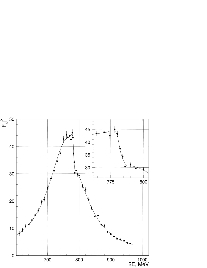
Figure 25: Fit of the CMD-2 (94, 95) pion form factor data according to GS and HLS models. Both theoretical curves are presented, but they are indistinguishable

	GS model	HLS model
$\mathrm{M}_{\rho}$, MeV	$775.28\pm 0.61\pm 0.20$	$774.57\pm 0.60\pm 0.20$
$\Gamma_{\rho}$, MeV	$147.70\pm 1.29\pm 0.40$	$147.65\pm 1.38\pm 0.20$
$Br(\omega\rightarrow\pi^{+}\pi^{-})$, %	$1.31\pm 0.23\pm 0.02$	$1.32\pm 0.23\pm 0.02$
$\Gamma(\rho\rightarrow e^{+}e^{-})$, keV	$6.93\pm 0.11\pm 0.10$	$6.89\pm 0.12\pm 0.10$
$\beta$ (GS)	$-0.0849\pm 0.0053\pm 0.0050$	—
$a$ (HLS)	—	$2.381\pm 0.016\pm 0.016$
$\chi^{2}/n$	0.77	0.78

Table 3: The results of fit of the CMD-2 (94,95) pion form factor data by GS and HLS models

3.4 Hadronic Contribution to (g-2)_μ

We’ll now estimate the implication of our results for the value and uncertainty of $a_{\mu}^{had}$ - the hadronic contribution to (g-2)_μ. To this end we’ll choose the c.m.energy range near the $\rho$-meson peak (from 630 to 810 MeV) which gives the dominant contribution to the muon anomaly and where good data are available from previous measurements by the OLYA and CMD groups [6] as well as by the DM1 detector [26]. Table 4 presents results of our calculations of $a_{\mu}^{had}$ performed by direct integration of the experimental data over the energy range above. The calculation used the following procedure: first we integrated the data of each group over the chosen energy range. Since measurements at different energy points are independent, the squared statistical error of the integral can be obtained by summing statistical errors squared of each energy point. After that the systematic uncertainty which is believed to be an overall normalization uncertainty is added quadratically. Contributions of separate groups are subject to weighted averaging taking into account if necessary a scale factor [18]. Such a procedure implies an assumption that systematical uncertainties are uncorrelated since they refer to different measurements.

Data	a${}_{\mu}^{had}$, 10-10	Total error, 10-10
Old	284.2 $\pm$ 3.8 $\pm$ 7.1	8.1
New	292.5 $\pm$ 2.2 $\pm$ 4.1	4.7
Old+New	290.3 $\pm$ 1.9 $\pm$ 3.6	4.1

Table 4: Hadronic contributions to (g-2)_μ, coming from the c.m.energy range near the $\rho$-meson peak.

The first line gives the average of three independent estimates based on the data of OLYA, CMD and MD1 while the second one presents the corresponding value for the CMD-2 data. The third line of the Table is the average based on the four independent estimates above. For convenience, we list separately the statistical and systematic uncertainties in the second column while the third one gives the total error obtained by adding them quadratically. One can see that the estimate based on the CMD-2 data is in good agreement with that coming from the old data. Note also the significant improvement of both statistical and systematic uncertainties compared to the previous measurements. The combined result (old plus new data) is a factor of two more precise than before.

4 Conclusion

A new measurement of the pion form factor in the center-of-mass energy range $0.61-0.96$ GeV is presented. The statistical error is about the same as for all previous $e^{+}e^{-}$ data, but the systematic error is a few times smaller. The results are based only on part of the experimental data taken by CMD-2. There are several reasons why this data set was treated as independent. First, a different approach in data analysis is required for the data taken in the center-of-mass energy range below $0.6$ GeV and above $1.0$ GeV (runs 4 and 5 in table 1). Second, the data taking conditions were significantly different in 1998 (run 6 in table 1), when the data was taken in the same $0.61-0.96$ GeV energy range. As a result, the systematic errors for these runs will be different than for the data presented here. Therefore we prefer to present separate results for different groups of runs.

The fit of the pion form factor based on the Gounaris-Sakurai and the Hidden Local Symmetry parametrizations was performed. For the final values we prefer the Gounaris-Sakurai parametrization as it was traditionally used for the determination of the $\rho$-meson parameters (see [6] and [21]). The difference between the results of the fit in two models is always smaller than the experimental error (Table 3), therefore the “model” error is not specified. We give as the final results the following, where the first error is statistical and the second one is systematic:

$$\left\{\begin{array}[]{ll}\mathrm{M}_{\rho}\,(\mathrm{MeV})&=775.28\pm 0.61\pm 0.20,\vphantom{\Bigl{(}\Bigr{)}}\\ \Gamma_{\rho}\,(\mathrm{MeV})&=147.70\pm 1.29\pm 0.40,\vphantom{\Bigl{(}\Bigr{)}}\\ \Gamma(\rho\rightarrow e^{+}e^{-})\,(\mathrm{keV})&=6.93\pm 0.11\pm 0.10,\vphantom{\Bigl{(}\Bigr{)}}\\ Br(\omega\rightarrow\pi^{+}\pi^{-})&=(1.31\pm 0.23)\%.\vphantom{\Bigl{(}\Bigr{)}}\end{array}\right.$$ (29)

It has also been shown that the improvement of the experimental precision, particularly of the systematic uncertainties, can be crucial for the high precision calculation of the hadronic contribution to the muon anomaly.

With the progress of analysis of the rest available data we hope to reduce the systematic error for the data presented here by additional factor of two. Important part of this improvement is the development of the new approach to the radiative corrections calculation with the ultimate goal to reduce the corresponding systematic error to $(0.3-0.5)\%$ level. Using the high statistics taken in 1998, it will be possible to perform the detailed analysis of small systematic effects.

The authors are grateful to the staff of VEPP-2M for excellent performance of the collider, to all engineers and technicians who participated in the design, commissioning and operation of CMD-2. We acknowledge the contribution to the experiment at the earlier stages of our colleagues V.A.Monich, A.E.Sher, V.G.Zavarzin and W.A.Worstell. Special thanks are due to N.N.Achasov, A.B.Arbuzov, M.Benayoun, V.L.Chernyak, V.S.Fadin, F.Jegerlehner, E.A.Kuraev, A.I.Milstein and G.N.Shestakov for useful discussions and permanent interest.

This work is supported in part by grants RFBR-98-02-17851, INTAS 96-0624 and DOE DEFG0291ER40646.

References

- [1] T.Kinoshita, B.Niẑić and Y.Okamoto, Phys. Rev. D31 (1985) 2108.
- [2] S.Eidelman and F.Jegerlehner, Z.Phys. C67 (1995) 585.
- [3] D.H.Brown and W.A.Worstell, Phys. Rev. D54 (1996) 3237.
- [4] C.Timmermans et al., Proc. of the International Conference on High Energy Physics (ICHEP), July 1998, Vancouver, Canada.
- [5] V.V.Anashin et al., Preprint INP 84-114, Novosibirsk (1984).
- [6] L.M.Barkov et al., Nucl. Phys. B256 (1985) 365.
- [7] E.V.Anashkin et al., ICFA Instrumentation Bulletin 5 (1988).
- [8] G.A.Aksenov et al., Preprint INP 85-118, Novosibirsk (1985).
- [9] R.R.Akhmetshin et al., Preprint BINP 99-11, Novosibirsk, 1999.
- [10] W.T.Eadie et al., “Statistical methods in experimental physics”, North-Holland publishing company, Amsterdam-London, 1971.
- [11] F.A.Berends and R.Kleiss, Nucl. Phys. B228 (1983) 537.
- [12] E.A.Kuraev, V.S.Fadin, Sov. J. Nucl. Phys. 41 (1985) 466.
- [13] A.B.Arbuzov, E.A.Kuraev et al., Preprint JHEP 10 (1997).
- [14] GEANT — Detector Description and Simulation Tool, CERN, 1994.
- [15] P.A.Aarnio et al., Fluka user’s guide. Technical Report TIS-RP-190, CERN, 1987, 1990.
- [16] H.C.Fesefeldt, Simulation of hadronic showers, physics and applications. Technical report PITHA 85-02, III Physikalisches Institut, RWTH Aachen Physikzentrum, 5100 Aachen, Germany, September 1985.
- [17] P.Krokovny, Bachelor Thesis, Novosibirsk State University, 1998.
- [18] C.Caso et al., Eur. Phys. J. C3 (1998) 1.
- [19] A.Lysenko et al., Nucl. Instr. Meth.A359 (1995) 419.
- [20] E.V.Anashkin et al., Nucl. Instr. Meth.A379 (1996) 432.
- [21] R.Barate et al., Z.Phys. C76 (1997) 15.
- [22] M. Benayoun et al., Eur.Phys.J. C2 (1998) 269.
- [23] G.J.Gounaris and J.J.Sakurai, Phys. Rev. Lett. 21 (1968) 244.
- [24] M.Bando et al., Phys.Rev.Lett. 54 (1985) 1215.
- [25] H.B.O’Connell et al., Prog. Nucl. Part. Phys. 39 (1997) 201.
- [26] A.Quenzer et al., Phys. Lett. 76B (1978) 512.