EUROPEAN ORGANIZATION FOR PARTICLE PHYSICS

CERN–EP/99–042

3 March 1999

Study of Fermion Pair Production
in $\mathrm{e}^{+}e^{-}$ Collisions at 130–183 GeV

The ALEPH Collaboration

Abstract

The cross sections and forward-backward asymmetries of hadronic and leptonic events produced in ${\mathrm{e}}^{+}{\mathrm{e}}^{-}$ collisions at centre-of-mass energies from 130 to 183 GeV are presented. Results for ${\mathrm{e}}^{+}{\mathrm{e}}^{-}$, ${\mu^{+}\mu^{-}}$, ${\tau^{+}\tau^{-}}$, ${\mathrm{q}}\bar{\mathrm{q}}$, ${\mathrm{b}}\bar{\mathrm{b}}$ and ${\mathrm{c}}\bar{\mathrm{c}}$ production show no significant deviation from the Standard Model predictions. This enables constraints to be set upon physics beyond the Standard Model such as four-fermion contact interactions, leptoquarks, $\mathrm{Z}^{\prime}$ bosons and R-parity violating squarks and sneutrinos. Limits on the energy scale $\Lambda$ of ${\mathrm{e}}^{+}{\mathrm{e}}^{-}$${\mathrm{f}}\bar{\mathrm{f}}$ contact interactions are typically in the range from 2 to 10 TeV. Limits on R-parity violating sneutrinos reach masses of a few hundred GeV/$c^{2}$ for large values of their Yukawa couplings.

To be submitted to Euro. Phys. J. C

The ALEPH Collaboration

R. Barate, D. Decamp, P. Ghez, C. Goy, S. Jezequel, J.-P. Lees, F. Martin, E. Merle, M.-N. Minard, B. Pietrzyk

Laboratoire de Physique des Particules (LAPP), IN²P³-CNRS, F-74019 Annecy-le-Vieux Cedex, France

R. Alemany, M.P. Casado, M. Chmeissani, J.M. Crespo, E. Fernandez, M. Fernandez-Bosman, Ll. Garrido,¹⁵ E. Graugès, A. Juste, M. Martinez, G. Merino, R. Miquel, Ll.M. Mir, P. Morawitz, A. Pacheco, I.C. Park, I. Riu

Institut de Física d’Altes Energies, Universitat Autònoma de Barcelona, 08193 Bellaterra (Barcelona), E-Spain⁷

A. Colaleo, D. Creanza, M. de Palma, G. Gelao, G. Iaselli, G. Maggi, M. Maggi, S. Nuzzo, A. Ranieri, G. Raso, F. Ruggieri, G. Selvaggi, L. Silvestris, P. Tempesta, A. Tricomi,³ G. Zito

Dipartimento di Fisica, INFN Sezione di Bari, I-70126 Bari, Italy

X. Huang, J. Lin, Q. Ouyang, T. Wang, Y. Xie, R. Xu, S. Xue, J. Zhang, L. Zhang, W. Zhao

Institute of High-Energy Physics, Academia Sinica, Beijing, The People’s Republic of China⁸

D. Abbaneo, U. Becker,¹⁹ G. Boix,⁶ M. Cattaneo, V. Ciulli, G. Dissertori, H. Drevermann, R.W. Forty, M. Frank, F. Gianotti, A.W. Halley, J.B. Hansen, J. Harvey, P. Janot, B. Jost, I. Lehraus, O. Leroy, C. Loomis, P. Maley, P. Mato, A. Minten, A. Moutoussi, F. Ranjard, L. Rolandi, D. Rousseau, D. Schlatter, M. Schmitt,²⁰ O. Schneider,²³ W. Tejessy, F. Teubert, I.R. Tomalin, E. Tournefier, M. Vreeswijk, A.E. Wright

European Laboratory for Particle Physics (CERN), CH-1211 Geneva 23, Switzerland

Z. Ajaltouni, F. Badaud G. Chazelle, O. Deschamps, S. Dessagne, A. Falvard, C. Ferdi, P. Gay, C. Guicheney, P. Henrard, J. Jousset, B. Michel, S. Monteil, J-C. Montret, D. Pallin, P. Perret, F. Podlyski

Laboratoire de Physique Corpusculaire, Université Blaise Pascal, IN²P³-CNRS, Clermont-Ferrand, F-63177 Aubière, France

J.D. Hansen, J.R. Hansen, P.H. Hansen, B.S. Nilsson, B. Rensch, A. Wäänänen

Niels Bohr Institute, 2100 Copenhagen, DK-Denmark⁹

G. Daskalakis, A. Kyriakis, C. Markou, E. Simopoulou, A. Vayaki

Nuclear Research Center Demokritos (NRCD), GR-15310 Attiki, Greece

A. Blondel, J.-C. Brient, F. Machefert, A. Rougé, M. Swynghedauw, R. Tanaka, A. Valassi,¹² H. Videau

Laboratoire de Physique Nucléaire et des Hautes Energies, Ecole Polytechnique, IN²P³-CNRS, F-91128 Palaiseau Cedex, France

E. Focardi, G. Parrini, K. Zachariadou

Dipartimento di Fisica, Università di Firenze, INFN Sezione di Firenze, I-50125 Firenze, Italy

R. Cavanaugh, M. Corden, C. Georgiopoulos

Supercomputer Computations Research Institute, Florida State University, Tallahassee, FL 32306-4052, USA ^13,14

A. Antonelli, G. Bencivenni, G. Bologna,⁴ F. Bossi, P. Campana, G. Capon, F. Cerutti, V. Chiarella, P. Laurelli, G. Mannocchi,⁵ F. Murtas, G.P. Murtas, L. Passalacqua, M. Pepe-Altarelli¹

Laboratori Nazionali dell’INFN (LNF-INFN), I-00044 Frascati, Italy

M. Chalmers, L. Curtis, J.G. Lynch, P. Negus, V. O’Shea, B. Raeven, C. Raine, D. Smith, P. Teixeira-Dias, A.S. Thompson, J.J. Ward

Department of Physics and Astronomy, University of Glasgow, Glasgow G12 8QQ,United Kingdom¹⁰

O. Buchmüller, S. Dhamotharan, C. Geweniger, P. Hanke, G. Hansper, V. Hepp, E.E. Kluge, A. Putzer, J. Sommer, K. Tittel, S. Werner,¹⁹ M. Wunsch

Institut für Hochenergiephysik, Universität Heidelberg, D-69120 Heidelberg, Germany¹⁶

R. Beuselinck, D.M. Binnie, W. Cameron, P.J. Dornan,¹ M. Girone, S. Goodsir, N. Marinelli, E.B. Martin, J. Nash, J. Nowell, A. Sciabà, J.K. Sedgbeer, P. Spagnolo, E. Thomson, M.D. Williams

Department of Physics, Imperial College, London SW7 2BZ, United Kingdom¹⁰

V.M. Ghete, P. Girtler, E. Kneringer, D. Kuhn, G. Rudolph

Institut für Experimentalphysik, Universität Innsbruck, A-6020 Innsbruck, Austria¹⁸

A.P. Betteridge, C.K. Bowdery, P.G. Buck, P. Colrain, G. Crawford, G. Ellis, A.J. Finch, F. Foster, G. Hughes, R.W.L. Jones, N.A. Robertson, M.I. Williams

Department of Physics, University of Lancaster, Lancaster LA1 4YB, United Kingdom¹⁰

P. van Gemmeren, I. Giehl, F. Hölldorfer, C. Hoffmann, K. Jakobs, K. Kleinknecht, M. Kröcker, H.-A. Nürnberger, G. Quast, B. Renk, E. Rohne, H.-G. Sander, S. Schmeling, H. Wachsmuth C. Zeitnitz, T. Ziegler

Institut für Physik, Universität Mainz, D-55099 Mainz, Germany¹⁶

J.J. Aubert, C. Benchouk, A. Bonissent, J. Carr,¹ P. Coyle, A. Ealet, D. Fouchez, F. Motsch, P. Payre, M. Talby, M. Thulasidas, A. Tilquin

Centre de Physique des Particules, Faculté des Sciences de Luminy, IN²P³-CNRS, F-13288 Marseille, France

M. Aleppo, M. Antonelli, F. Ragusa

Dipartimento di Fisica, Università di Milano e INFN Sezione di Milano, I-20133 Milano, Italy.

R. Berlich, V. Büscher, H. Dietl, G. Ganis, K. Hüttmann, G. Lütjens, C. Mannert, W. Männer, H.-G. Moser, S. Schael, R. Settles, H. Seywerd, H. Stenzel, W. Wiedenmann, G. Wolf

Max-Planck-Institut für Physik, Werner-Heisenberg-Institut, D-80805 München, Germany

P. Azzurri, J. Boucrot, O. Callot, S. Chen, M. Davier, L. Duflot, J.-F. Grivaz, Ph. Heusse, A. Jacholkowska, M. Kado, J. Lefrançois, L. Serin, J.-J. Veillet, I. Videau,¹ J.-B. de Vivie de Régie, D. Zerwas

Laboratoire de l’Accélérateur Linéaire, Université de Paris-Sud, IN²P³-CNRS, F-91898 Orsay Cedex, France

G. Bagliesi, S. Bettarini, T. Boccali, C. Bozzi,²⁴ G. Calderini, R. Dell’Orso, I. Ferrante, A. Giassi, A. Gregorio, F. Ligabue, A. Lusiani, P.S. Marrocchesi, A. Messineo, F. Palla, G. Rizzo, G. Sanguinetti, G. Sguazzoni, R. Tenchini, C. Vannini, A. Venturi, P.G. Verdini

Dipartimento di Fisica dell’Università, INFN Sezione di Pisa, e Scuola Normale Superiore, I-56010 Pisa, Italy

G.A. Blair, J. Coles, G. Cowan, M.G. Green, D.E. Hutchcroft, L.T. Jones, T. Medcalf, J.A. Strong, J.H. von Wimmersperg-Toeller

Department of Physics, Royal Holloway & Bedford New College, University of London, Surrey TW20 OEX, United Kingdom¹⁰

D.R. Botterill, R.W. Clifft, T.R. Edgecock, P.R. Norton, J.C. Thompson

Particle Physics Dept., Rutherford Appleton Laboratory, Chilton, Didcot, Oxon OX11 OQX, United Kingdom¹⁰

B. Bloch-Devaux, P. Colas, B. Fabbro, G. Faïf, E. Lançon, M.-C. Lemaire, E. Locci, P. Perez, H. Przysiezniak, J. Rander, J.-F. Renardy, A. Rosowsky, A. Trabelsi,²¹ B. Tuchming, B. Vallage

CEA, DAPNIA/Service de Physique des Particules, CE-Saclay, F-91191 Gif-sur-Yvette Cedex, France¹⁷

S.N. Black, J.H. Dann, H.Y. Kim, N. Konstantinidis, A.M. Litke, M.A. McNeil, G. Taylor

Institute for Particle Physics, University of California at Santa Cruz, Santa Cruz, CA 95064, USA²²

C.N. Booth, S. Cartwright, F. Combley, P.N. Hodgson, M.S. Kelly, M. Lehto, L.F. Thompson

Department of Physics, University of Sheffield, Sheffield S3 7RH, United Kingdom¹⁰

K. Affholderbach, A. Böhrer, S. Brandt, C. Grupen, A. Misiejuk, G. Prange, U. Sieler

Fachbereich Physik, Universität Siegen, D-57068 Siegen, Germany¹⁶

G. Giannini, B. Gobbo

Dipartimento di Fisica, Università di Trieste e INFN Sezione di Trieste, I-34127 Trieste, Italy

J. Putz, J. Rothberg, S. Wasserbaech, R.W. Williams

Experimental Elementary Particle Physics, University of Washington, WA 98195 Seattle, U.S.A.

S.R. Armstrong, E. Charles, P. Elmer, D.P.S. Ferguson, Y. Gao, S. González, T.C. Greening, O.J. Hayes, H. Hu, S. Jin, P.A. McNamara III, J.M. Nachtman,² J. Nielsen, W. Orejudos, Y.B. Pan, Y. Saadi, I.J. Scott, J. Walsh, Sau Lan Wu, X. Wu, G. Zobernig

Department of Physics, University of Wisconsin, Madison, WI 53706, USA¹¹

1 Introduction

In the period 1995-97, the centre-of-mass energy of the LEP ${\mathrm{e}}^{+}{\mathrm{e}}^{-}$ collider was increased in five energy steps from 130 to 183 GeV, so opening a new energy regime for electroweak cross section and asymmetry measurements. Such measurements provide a test of the Standard Model (SM) and allow one to place limits on possible extensions to it.

This paper begins by providing in Section 2 the definitions of cross section and asymmetry used here. A brief description of the ALEPH detector is given in Section 3 and details of the luminosity measurement and data/Monte Carlo samples in Section 4.

Section 5 describes the measurement of the ${\mathrm{q}}\bar{\mathrm{q}}$ cross section. It also explores heavy quark production, providing measurements of $R_{\mathrm{b}}$ ($R_{\mathrm{c}}$) which are here defined as the ratio of the ${\mathrm{b}}\bar{\mathrm{b}}$ (${\mathrm{c}}\bar{\mathrm{c}}$) cross section to the total ${\mathrm{q}}\bar{\mathrm{q}}$ cross section. Constraints on ${\mathrm{q}}\bar{\mathrm{q}}$ forward-backward asymmetries are obtained using jet charge measurements. In Section 6, cross section and asymmetry results are reported for the three lepton species.

Based on these results, Section 7 gives limits on extensions to the SM involving contact interactions, R-parity violating sneutrinos, leptoquarks, $\mathrm{Z}^{\prime}$ bosons and R-parity violating squarks.

2 Definition of Cross Section and Asymmetry

Cross section results for all fermion species are provided for

1. the inclusive process, comprising all events with $\sqrt{s^{\prime}/s}>0.1$, so including events having hard initial state radiation (ISR).

2. the exclusive process, comprising all events with $\sqrt{s^{\prime}/s}>0.9$, so excluding radiative events, such as those in which a return to the Z resonance occurs.

Here, the variable $s$ is the square of the centre-of-mass energy. For leptonic final states the variable $s^{\prime}$ is defined as the square of the mass of the outgoing lepton pair. For hadronic final states $s^{\prime}$ is defined as the mass squared of the Z/$\gamma^{*}$ propagator. This latter choice is necessary, because as a result of gluon radiation, (which may occur before or after final state photon radiation), the mass of the outgoing quark pair is not well defined.

Interference effects between ISR and final state radiative (FSR) photons affect the exclusive cross sections at the level of a few percent and are not accurately described by existing Monte Carlo (MC) generators. They are particularly prominent when the outgoing fermions make a small angle to the incoming ${\mathrm{e}}^{+}{\mathrm{e}}^{-}$ beams. To reduce uncertainties related to this, the exclusive cross section and asymmetry results presented here are defined so as to include only the polar angle region $|{\cos\theta}|<0.95$, where $\theta$ is the polar angle of the outgoing fermion. This is unnecessary for the inclusive cross sections, since they are relatively insensitive to radiative photons. The inclusive results are therefore defined to include the full angular acceptance.

When selecting events experimentally, the variable $s^{\prime}_{m}$ is used, which provides a good approximation to $s^{\prime}$ when only one ISR photon is present:

$$s^{\prime}_{m}\;=\;\frac{\sin\theta_{1}\;+\;\sin\theta_{2}\;-\;|{\sin(\theta_{1}+\theta_{2})}|}{\sin\theta_{1}\;+\;\sin\theta_{2}\;+\;|{\sin(\theta_{1}+\theta_{2})}|}\;\times\;s~{}.$$ (1)

Here $\theta_{1}$ and $\theta_{2}$ are the angles of the final state fermions f and $\bar{\mathrm{f}}$ measured with respect to the direction of the incoming e^- beam or with respect to the direction of a photon seen in the apparatus and consistent with ISR. If two or more such photons are found, the angles are measured with respect to the sum of their three-momenta. The fermion flight directions are determined in electron and muon pair events simply from the directions of the reconstructed tracks, in tau pair events from the jets reconstructed from the visible tau decay products, and in hadronic events from the jets formed when forcing the event into two jets after removing isolated, high energy photons detected in the apparatus.

If an event contains two or more ISR photons, then unless these photons all go in the same direction, the variable $s^{\prime}_{m}$ ceases to be a good approximation to $s^{\prime}$. Such events can pass the exclusive selection by being reconstructed with $\sqrt{s^{\prime}_{m}/s}>0.9$, but nonetheless have $\sqrt{s^{\prime}/s}<0.9$. They are called ‘radiative background’.

For dilepton events, the differential cross section is measured as a function of the angle $\theta^{*}$, defined by

$$\cos\theta^{*}=\frac{\sin\frac{1}{2}(\theta_{+}-\theta_{-})}{\sin\frac{1}{2}(\theta_{+}+\theta_{-})}~{},$$ (2)

where $\theta_{-}$ and $\theta_{+}$ are the angles of the negatively and positively charged leptons, respectively, with respect to the incoming e^- beam. The angle $\theta^{*}$ corresponds to the scattering angle between the incoming e^- and the outgoing l^-, measured in the ${\mathrm{l}}^{+}{\mathrm{l}}^{-}$ rest frame, provided that no large-angle ISR photons are present.

The forward-backward asymmetries are determined from the formula

$$\mbox{$A_{\mathrm{F}B}^{\mathrm{}}$}=\frac{\sigma_{F}-\sigma_{B}}{\sigma_{F}+\sigma_{B}}~{},$$ (3)

where $\sigma_{F}$ and $\sigma_{B}$ are the cross sections to produce events with the negatively charged lepton in the forward ($\theta_{-}<90^{\circ}$) and backward ($\theta_{-}>90^{\circ}$) hemispheres, respectively, defined in the same limited angular acceptance as given above. Determining the forward-backward asymmetries from this formula avoids any specific assumption about the angular dependence of the differential cross section.

3 The ALEPH Detector

The ALEPH detector and performance are fully described in [1] and [2]. In October 1995, the silicon vertex detector (VDET) described in these papers was replaced by an improved detector [3], which is used for the analyses presented here. A brief description of the ALEPH detector follows.

The main tracking detector is a time projection chamber (TPC) lying between radii of 30 and 180 cm from the beam axis. It provides up to 21 three-dimensional coordinates per track. Inside the TPC is a small drift chamber (ITC) and within this, the new VDET. The latter has two layers of silicon, each providing three-dimensional coordinates. All three tracking detectors contribute coordinates to tracks for polar angles to the beam axis up to $|{\cos\theta}|<0.95$. They are immersed in a 1.5 T axial magnetic field provided by a superconducting solenoid. This allows the momentum $p$ of charged tracks to be measured with a resolution of $\sigma(p)/p=6\times 10^{-4}p_{T}\oplus 0.005$ (where $p_{T}$ is the momentum component perpendicular to the beam axis in GeV/$c$). The three-dimensional impact parameter resolution is measured with an accuracy of $(34+70/p)\times(1+1.6\cos^{4}\theta)$ $\mu$m (where $p$ is measured in GeV/$c$).

Between the tracking detectors and the solenoid is an electromagnetic calorimeter (ECAL), which provides identification of electrons and photons, and measures their energies $E$ with a resolution of $\sigma(E)/E=0.18/\sqrt{E({\mathrm{G}eV})}+0.009$. Outside the solenoid, is a hadron calorimeter (HCAL), which, combined with the ECAL, measures the energy of hadrons with a resolution of $\sigma(E)/E=0.85/\sqrt{E({\mathrm{G}eV})}$. The HCAL is also used for muon identification, together with muon chambers lying outside it. The ECAL and HCAL acceptances extend down to polar angles of 190 and 100 mrad to the beam axis, respectively.

The luminosity is measured with a lead/proportional-chamber electromagnetic calorimeter (LCAL) covering the small angle region between 46 and 122 mrad from the beam axis. A tungsten/silicon electromagnetic calorimeter (SICAL) covering the angular range from 24 to 58 mrad is used to provide a cross-check.

In general, charged tracks are considered good for the analyses presented here if they originate within a cylinder of radius 2 cm and length 10 cm, centered at the interaction point, and whose axis is parallel to the beam axis. They must also have at least four TPC hits, a momentum larger than 0.1 GeV/$c$ and a polar angle to the beam axis satisfying $|{\cos\theta}|<0.95$.

By relating charged tracks to energy deposits found in the calorimeters and using photon, electron and muon identification information, a list of charged and neutral energy flow particles [2] is created for each event and used in the following analyses.

4 Data and Monte Carlo Samples and the Luminosity Measurement

The data used were taken at five centre-of-mass energies which are given in Table 1. This table also shows the integrated luminosity recorded at each energy point, together with its statistical and systematic uncertainties.

Table 1: Centre-of-mass energies and integrated luminosities of the high energy data samples. The two uncertainties quoted on each integrated luminosity correspond to its statistical and systematic uncertainty respectively.

Energy (GeV)	Luminosity (pb-1)
130.2	$~{}6.03\pm 0.03\pm 0.05$
136.2	$~{}6.10\pm 0.03\pm 0.05$
161.3	$11.08\pm 0.04\pm 0.07$
172.1	$10.65\pm 0.05\pm 0.06$
182.7	$56.78\pm 0.11\pm 0.29$

For analyses relying heavily on the VDET, such as the study of ${\mathrm{b}}\bar{\mathrm{b}}$ production, data collected at 130 and 136 GeV in 1995 are discarded, since the new VDET was not fully installed. However, data taken at these two energy points in 1997, corresponding to integrated luminosities of 3.30 and 3.51 $\mathrm{pb}^{-1}$, respectively, are used.

The luminosity is measured using the LCAL calorimeter following the analysis procedure described in Ref. [4], with a slightly reduced acceptance due to the shadowing of the LCAL detector by the SICAL below 59 mrad. The systematic uncertainty on the luminosity, which is assumed to be fully correlated between the different energy points, includes a theoretical uncertainty, estimated to be 0.25% [5] from the BHLUMI [6] Monte Carlo generator. The luminosity measurement is checked by comparison with the luminosity measured independently using the SICAL detector. The two are consistent within the estimated uncertainties.

Samples of Monte Carlo events were produced as follows. The generator BHWIDE v1.01 [7] is used for the electron pair channel and KORALZ v4.2 [8] for the muon and tau pair channels. Simulation of diquark events relies on production of the initial ${\mathrm{q}}\bar{\mathrm{q}}$ system and accompanying ISR photons with either KORALZ or PYTHIA v5.7 [9]. The simulation of FSR and fragmentation is then carried out with the program JETSET v7.4 [9]. The PYTHIA generator is also used for four-fermion processes such as the Z pair and Ze⁺e^- channels. The programs PHOT02 [10], HERWIG v5.9 [11] and PYTHIA are used to generate the two-photon events. Finally, backgrounds from W pair production are studied using the generators KORALW v1.21 [12] and EXCALIBUR [13].

5 Hadronic Final States

Section 5.1 describes the measurement of the ${\mathrm{q}}\bar{\mathrm{q}}$ cross section. Sections 5.2 and 5.3 study heavy quark production, providing measurements of $R_{\mathrm{b}}$ ($R_{\mathrm{c}}$) which are here defined as the ratio of the ${\mathrm{b}}\bar{\mathrm{b}}$ (${\mathrm{c}}\bar{\mathrm{c}}$) cross section to the total ${\mathrm{q}}\bar{\mathrm{q}}$ cross section. The measured values of $R_{\mathrm{b}}$ ($R_{\mathrm{c}}$) are statistically independent of the ${\mathrm{q}}\bar{\mathrm{q}}$ cross section measurement. Furthermore, by measuring these ratios, rather than the ${\mathrm{b}}\bar{\mathrm{b}}$ and ${\mathrm{c}}\bar{\mathrm{c}}$ cross sections, one benefits from the cancellation of some systematic uncertainties. Section 5.4 places constraints upon ${\mathrm{q}}\bar{\mathrm{q}}$ forward-backward asymmetries using a jet charge technique applied to b-enriched and b-depleted event samples.

5.1 The Hadronic Cross Section

The hadronic event selection begins by requiring events to have at least seven good charged tracks. The energy flow particles are then clustered into jets using the JADE algorithm [14] with a clustering parameter $y_{\mathrm{c}ut}$ of 0.008 . Thin, low multiplicity jets with an electromagnetic energy content of at least 90% and an energy of more than 10 GeV are considered to be ISR photon candidates. The visible mass $M_{\mathrm{v}is}$ of the event is then measured using charged and neutral energy flow particles, but excluding these photons and energy flow particles which make an angle of less than $2^{\circ}$ to the beam axis. The distribution of $M_{\mathrm{v}is}$ is shown in Fig. 1 for data taken at 183 GeV. It is required to be more than 50 GeV/$c^{2}$.

The inclusive selection makes the additional requirement that $\sqrt{s^{\prime}_{m}/s}>0.1$. There is actually negligible acceptance for events with $0.1<\sqrt{s^{\prime}/s}<0.3$ as a result of the cut on $M_{\mathrm{v}is}$. The inclusive cross sections are therefore extrapolated down to $\sqrt{s^{\prime}/s}=0.1$ using the KORALZ generator.

The exclusive selection requires $\sqrt{s^{\prime}_{m}/s}>0.9$. Here $s^{\prime}_{m}$ is determined from the reconstructed jet directions, when the event is clustered into two jets, after first removing reconstructed ISR photons. For the exclusive selection, these jets are required to have $|{\cos\theta}|<0.95$ . The $\sqrt{s^{\prime}_{m}/s}$ distributions for centre-of-mass energies of 130, 161, 172 and 183 GeV are displayed in Fig. 2, together with the expected background.

For the exclusive process, two additional cuts are then applied. Firstly, $M_{\mathrm{v}is}$  is required to exceed 70% of the centre-of-mass energy. This suppresses residual events with a radiative return to the Z. Such events can have $\sqrt{s^{\prime}_{m}/s}>0.9$ if they emit two or more ISR photons. Figure 3 shows $M_{\mathrm{v}is}$ for events with $\sqrt{s^{\prime}_{m}/s}>0.9$. The contribution from doubly radiative events is clearly seen at low masses. Secondly, when above the $\mathrm{W}^{+}W^{-}$ threshold, (i.e. $\sqrt{s}\geq 161$ GeV), about 80% of $\mathrm{W}^{+}W^{-}$ background is eliminated by requiring that the thrust of the event exceeds 0.85 . The thrust distribution is shown in Fig. 4.

Figure 1: Visible mass distribution at a centre-of-mass energy of 183 GeV for events having at least seven tracks. The white histogram shows the expected signal, whilst the hashed histograms give the expected contributions of the $\gamma\gamma$ and W pair backgrounds. The arrow indicates the cut used in the inclusive selection.

Figure 2: $\sqrt{s^{\prime}_{m}/s}$ distribution for hadronic events at centre-of-mass energies from 130 to 183 GeV. This is compared to the Monte Carlo expectations shown by the white histograms. The hashed areas correspond to background contributions and are dominated by W pair production. The distribution at 136 GeV is omitted because it closely resembles that at 130 GeV.

Figure 3: Visible mass distribution at 183 GeV centre-of-mass energy for hadronic events with $\sqrt{s^{\prime}_{m}/s}>0.9$. This is compared with Monte Carlo expectations shown by the white histogram. The hashed area represents the expected contribution from events with generated $\sqrt{s^{\prime}/s}<0.9$. The arrow indicates the cut used in the exclusive selection.

Figure 4: Thrust distribution at 183 GeV centre-of-mass energy for hadronic events with $\sqrt{s^{\prime}_{m}/s}>0.9$. The white histogram shows the expected signal and the hashed one corresponds to the W pair background. The arrow indicates the cut used in the exclusive selection.

The selection efficiencies are estimated using the KORALZ Monte Carlo samples. The efficiencies are given for all centre-of-mass energies in Table 2.

Table 2: Selection efficiencies and background fractions. For ${\mathrm{e}}^{+}{\mathrm{e}}^{-}$ production, numbers are given for (1) $-0.9<\cos\theta^{*}<0.9$ and (2) $-0.9<\cos\theta^{*}<0.7$.

$\sqrt{s^{\prime}/s}$	$\mathrm{E}_{cm}$	Event	Efficiency	Background
cut	(GeV)	type	(%)	(%)
0.1	130	${\mathrm{q}}\bar{\mathrm{q}}$	$89.6\pm 0.9$	$~{}2.4\pm 0.3$
		$\mu^{+}\mu^{-}$	$78.8\pm 1.6$	$~{}0.4\pm 0.1$
		$\tau^{+}\tau^{-}$	$55.3\pm 1.1$	$~{}5.7\pm 2.4$
	136	${\mathrm{q}}\bar{\mathrm{q}}$	$89.5\pm 0.7$	$~{}1.6\pm 0.2$
		$\mu^{+}\mu^{-}$	$78.8\pm 1.6$	$~{}0.5\pm 0.1$
		$\tau^{+}\tau^{-}$	$53.9\pm 1.3$	$~{}8.9\pm 4.0$
	161	${\mathrm{q}}\bar{\mathrm{q}}$	$88.4\pm 0.6$	$~{}4.0\pm 0.1$
		$\mu^{+}\mu^{-}$	$76.5\pm 1.5$	$~{}3.3\pm 1.2$
		$\tau^{+}\tau^{-}$	$44.2\pm 1.4$	$~{}8.3\pm 4.0$
	172	${\mathrm{q}}\bar{\mathrm{q}}$	$87.3\pm 0.6$	$10.2\pm 0.1$
		$\mu^{+}\mu^{-}$	$75.6\pm 1.6$	$~{}4.1\pm 1.3$
		$\tau^{+}\tau^{-}$	$44.8\pm 1.0$	$11.3\pm 3.7$
	183	${\mathrm{q}}\bar{\mathrm{q}}$	$83.9\pm 0.7$	$17.8\pm 0.2$
		$\mu^{+}\mu^{-}$	$75.6\pm 1.6$	$~{}5.4\pm 1.2$
		$\tau^{+}\tau^{-}$	$47.4\pm 0.9$	$12.9\pm 2.6$
0.9	130	${\mathrm{q}}\bar{\mathrm{q}}$	$92.2\pm 1.0$	$~{}9.5\pm 0.3$
		${\mathrm{e}}^{+}{\mathrm{e}}^{-}$(1)	$90.0\pm 1.6$	$10.4\pm 0.9$
		${\mathrm{e}}^{+}{\mathrm{e}}^{-}$(2)	$95.5\pm 1.4$	$11.5\pm 1.0$
		$\mu^{+}\mu^{-}$	$95.1\pm 1.8$	$~{}3.3\pm 0.7$
		$\tau^{+}\tau^{-}$	$63.9\pm 1.6$	$11.9\pm 3.2$
	136	${\mathrm{q}}\bar{\mathrm{q}}$	$89.2\pm 0.8$	$~{}8.8\pm 0.4$
		${\mathrm{e}}^{+}{\mathrm{e}}^{-}$(1)	$90.6\pm 1.5$	$10.8\pm 1.0$
		${\mathrm{e}}^{+}{\mathrm{e}}^{-}$(2)	$96.9\pm 1.4$	$14.1\pm 1.6$
		$\mu^{+}\mu^{-}$	$95.1\pm 1.8$	$~{}3.3\pm 0.7$
		$\tau^{+}\tau^{-}$	$63.6\pm 1.5$	$15.9\pm 3.1$
	161	${\mathrm{q}}\bar{\mathrm{q}}$	$89.3\pm 0.7$	$~{}7.7\pm 0.3$
		${\mathrm{e}}^{+}{\mathrm{e}}^{-}$(1)	$89.1\pm 1.5$	$10.0\pm 0.9$
		${\mathrm{e}}^{+}{\mathrm{e}}^{-}$(2)	$94.8\pm 1.3$	$11.0\pm 1.3$
		$\mu^{+}\mu^{-}$	$96.0\pm 1.8$	$~{}4.5\pm 0.9$
		$\tau^{+}\tau^{-}$	$62.3\pm 1.7$	$~{}9.5\pm 2.7$
	172	${\mathrm{q}}\bar{\mathrm{q}}$	$90.2\pm 0.6$	$~{}6.4\pm 0.3$
		${\mathrm{e}}^{+}{\mathrm{e}}^{-}$(1)	$90.7\pm 1.5$	$10.7\pm 1.0$
		${\mathrm{e}}^{+}{\mathrm{e}}^{-}$(2)	$96.3\pm 1.2$	$11.9\pm 1.4$
		$\mu^{+}\mu^{-}$	$96.8\pm 1.8$	$~{}6.0\pm 1.3$
		$\tau^{+}\tau^{-}$	$64.6\pm 1.7$	$13.9\pm 3.8$
	183	${\mathrm{q}}\bar{\mathrm{q}}$	$85.9\pm 0.8$	$~{}9.2\pm 0.1$
		${\mathrm{e}}^{+}{\mathrm{e}}^{-}$(1)	$87.5\pm 1.4$	$10.9\pm 0.7$
		${\mathrm{e}}^{+}{\mathrm{e}}^{-}$(2)	$95.2\pm 1.2$	$12.4\pm 0.9$
		$\mu^{+}\mu^{-}$	$95.9\pm 1.8$	$~{}6.5\pm 1.3$
		$\tau^{+}\tau^{-}$	$67.9\pm 1.8$	$13.3\pm 3.0$

The uncertainties in the efficiencies arise from the statistical uncertainties on the Monte Carlo and also from a number of systematic effects, which are assessed as described below.

1. Uncertainties related to the simulation of ISR are estimated from the difference in the efficiencies determined from KORALZ and PYTHIA. Only the generator KORALZ simulates ISR using YFS exponentiation [8].

2. The overall ECAL energy calibration is determined each year, from Bhabha events recorded when running at the Z peak. Its uncertainty is estimated to be $\pm 0.9\%$, based upon a comparison of the detector response to low energy ($\approx 1$ GeV) electrons in $\gamma\gamma\rightarrow\mathrm{e}^{+}e^{-}$ events, with that to high energy electrons in Bhabha events. The calibration of the HCAL energy scale uses minimum ionizing particles. The statistical uncertainty on this calibration is $\pm 2\%$. These uncertainties on the calorimeter energy scales are considered to be uncorrelated from year to year.

3. The energy response to 45 GeV jets, in data and Monte Carlo events produced at the Z resonance, is compared and the difference parametrized as a function of polar angle to the beam axis. The selection efficiency is corrected using this parametrization. The systematic uncertainty due to the energy response is derived from the change in the measured cross section when this correction is applied. This uncertainty, which is the largest of the detector related ones, is considered to be correlated from year to year.

4. The measured polar angles of jets with respect to the beam axis can suffer from small systematic biases, particularly at low polar angles. These biases are studied using events produced at the Z resonance. Differences between the data and Monte Carlo are taken into account via their effect on $s^{\prime}_{m}$. The associated systematic uncertainty is given by the change in the measured cross section when applying these corrections. It is considered to be correlated from year to year.

The background fractions remaining after the selection are also given in Table 2. The uncertainty in these backgrounds receives contributions from the detector calibration and energy response, estimated as above. Additional uncertainties are studied as follows:

1. The two-photon background is simulated with the PYTHIA, PHOT02 and HERWIG generators. It is normalized to the data in the region $M_{\mathrm{v}is}<50$ GeV/$c^{2}$ (Fig. 1), and the difference between the expected cross section from PHOT02 and the normalized one is used to calculate the uncertainty on the process. This background dominates at centre-of-mass energies of 130 and 136 GeV.

2. Above the W pair production threshold, the $\mathrm{W}^{+}W^{-}$ background is estimated using KORALW. At 161 GeV the input cross section is taken from the theoretical expectation, computed with the GENTLE [15] program for a W mass of $80.39\pm 0.06$ GeV/$c^{2}$[16]. At 172 and 183 GeV the cross sections are taken from the average measurement of the four LEP experiments [16]. Uncertainties in the W pair cross sections are propagated to estimate the associated systematic uncertainties on the ${\mathrm{q}}\bar{\mathrm{q}}$ cross sections.

3. Other four-fermion backgrounds such as ZZ and Ze⁺e^- are estimated using PYTHIA and EXCALIBUR. They introduce only a $\pm 0.1$% systematic uncertainty on the exclusive ${\mathrm{q}}\bar{\mathrm{q}}$ cross section measurement.

4. Events where ISR occurs from the incoming electron and positron remain an important background for the exclusive selection. Systematic uncertainties on this background arise from the simulation of ISR photons and from the energy scale and response of the detector. These are already taken into account as described above.

The cross section measurements at each centre-of-mass energy are listed in Table 3, where they are compared with the SM predictions. These predictions are discussed in Section 7.1. For the exclusive results, the measurements and predictions refer to ${\mathrm{q}}\bar{\mathrm{q}}$ final states with $|{\cos\theta}|<0.95$, where $\theta$ is the polar angle of the quark with respect to the beam axis. A breakdown of contributions to the systematic uncertainties on the cross section measurements is given in Table 4.

Table 3: Measured cross sections with statistical and systematic uncertainties for different channels at centre-of-mass energies from 130 to 183 GeV. The SM predictions are also given, together with the number of selected events (before background subtraction). The exclusive cross sections correspond to the restricted angular range $|\cos\theta|<0.95$. For the Bhabha process, results are given for (1) $-0.9<\cos\theta^{*}<0.9$ and (2) $-0.9<\cos\theta^{*}<0.7$.

$\sqrt{s^{\prime}/s}$	$\mathrm{E}_{cm}$	Event	No.	$\sigma$	SM prediction
cut	(GeV)	type	Events	(pb)	(pb)
0.1	130	${\mathrm{q}}\bar{\mathrm{q}}$	1858	$335.6~{}\pm 7.9~{}\pm 4.5~{}$	327.0
		$\mu^{+}\mu^{-}$	110	$~{}22.5~{}\pm 2.2~{}\pm 0.5~{}$	21.9
		$\tau^{+}\tau^{-}$	94	$~{}25.9~{}\pm 2.9~{}\pm 0.6~{}$	21.9
	136	${\mathrm{q}}\bar{\mathrm{q}}$	1558	$280.8~{}\pm 7.2~{}\pm 3.7~{}$	269.8
		$\mu^{+}\mu^{-}$	103	$~{}20.4~{}\pm 2.1~{}\pm 0.5~{}$	18.7
		$\tau^{+}\tau^{-}$	67	$~{}17.8~{}\pm 2.5~{}\pm 0.5~{}$	18.6
	161	${\mathrm{q}}\bar{\mathrm{q}}$	1520	$149.0~{}\pm 4.0~{}\pm 1.7~{}$	147.6
		$\mu^{+}\mu^{-}$	107	$~{}12.2~{}\pm 1.2~{}\pm 0.3~{}$	11.2
		$\tau^{+}\tau^{-}$	78	$~{}14.6~{}\pm 1.8~{}\pm 0.3~{}$	11.2
	172	${\mathrm{q}}\bar{\mathrm{q}}$	1270	$122.6~{}\pm 3.8~{}\pm 1.2~{}$	122.8
		$\mu^{+}\mu^{-}$	74	$~{}~{}8.8~{}\pm 1.1~{}\pm 0.2~{}$	9.5
		$\tau^{+}\tau^{-}$	51	$~{}~{}9.5~{}\pm 1.5~{}\pm 0.3~{}$	9.5
	183	${\mathrm{q}}\bar{\mathrm{q}}$	6072	$104.8~{}\pm 1.6~{}\pm 0.9~{}$	104.4
		$\mu^{+}\mu^{-}$	406	$~{}~{}8.84\pm 0.47\pm 0.19$	8.22
		$\tau^{+}\tau^{-}$	241	$~{}~{}7.80\pm 0.58\pm 0.17$	8.22
0.9	130	${\mathrm{q}}\bar{\mathrm{q}}$	440	$~{}71.6~{}\pm 3.8~{}\pm 1.1~{}$	70.7
		${\mathrm{e}}^{+}{\mathrm{e}}^{-}$(1)	1186	$191.3~{}\pm 6.2~{}\pm 3.5~{}$	186.7
		${\mathrm{e}}^{+}{\mathrm{e}}^{-}$(2)	274	$~{}41.1~{}\pm 2.8~{}\pm 0.9~{}$	39.0
		$\mu^{+}\mu^{-}$	48	$~{}~{}7.9~{}\pm 1.2~{}\pm 0.2~{}$	7.0
		$\tau^{+}\tau^{-}$	49	$~{}10.9~{}\pm 1.8~{}\pm 0.4~{}$	7.3
	136	${\mathrm{q}}\bar{\mathrm{q}}$	351	$~{}58.8~{}\pm 3.5~{}\pm 0.9~{}$	57.3
		${\mathrm{e}}^{+}{\mathrm{e}}^{-}$(1)	1051	$162.2~{}\pm 5.6~{}\pm 3.5~{}$	167.3
		${\mathrm{e}}^{+}{\mathrm{e}}^{-}$(2)	212	$~{}29.5~{}\pm 2.4~{}\pm 0.7~{}$	33.9
		$\mu^{+}\mu^{-}$	43	$~{}~{}6.9~{}\pm 1.1~{}\pm 0.2~{}$	6.1
		$\tau^{+}\tau^{-}$	27	$~{}~{}5.6~{}\pm 1.3~{}\pm 0.2~{}$	6.3
	161	${\mathrm{q}}\bar{\mathrm{q}}$	321	$~{}29.94\pm 1.8~{}\pm 0.4~{}$	30.7
		${\mathrm{e}}^{+}{\mathrm{e}}^{-}$(1)	1393	$119.7~{}\pm 3.7~{}\pm 2.3~{}$	119.0
		${\mathrm{e}}^{+}{\mathrm{e}}^{-}$(2)	302	$~{}25.6~{}\pm 1.7~{}\pm 0.5~{}$	24.8
		$\mu^{+}\mu^{-}$	50	$~{}~{}4.49\pm 0.69\pm 0.09$	3.88
		$\tau^{+}\tau^{-}$	44	$~{}~{}5.75\pm 0.96\pm 0.23$	4.01
	172	${\mathrm{q}}\bar{\mathrm{q}}$	271	$~{}26.4~{}\pm 1.7~{}\pm 0.4~{}$	25.1
		${\mathrm{e}}^{+}{\mathrm{e}}^{-}$(1)	1166	$107.8~{}\pm 3.5~{}\pm 2.1~{}$	102.5
		${\mathrm{e}}^{+}{\mathrm{e}}^{-}$(2)	268	$~{}23.0~{}\pm 1.6~{}\pm 0.5~{}$	21.5
		$\mu^{+}\mu^{-}$	29	$~{}~{}2.64\pm 0.53\pm 0.06$	3.32
		$\tau^{+}\tau^{-}$	26	$~{}~{}3.26\pm 0.74\pm 0.09$	3.43
	183	${\mathrm{q}}\bar{\mathrm{q}}$	1165	$~{}21.71\pm 0.70\pm 0.23$	21.1
		${\mathrm{e}}^{+}{\mathrm{e}}^{-}$(1)	5063	$~{}90.9~{}\pm 1.4~{}\pm 1.7~{}$	90.9
		${\mathrm{e}}^{+}{\mathrm{e}}^{-}$(2)	1171	$~{}18.99\pm 0.63\pm 0.36$	19.11
		$\mu^{+}\mu^{-}$	175	$~{}~{}2.98\pm 0.24\pm 0.06$	2.89
		$\tau^{+}\tau^{-}$	129	$~{}~{}2.90\pm 0.29\pm 0.09$	2.98

Table 4: Contributions to the systematic uncertainties on the ${\mathrm{q}}\bar{\mathrm{q}}$ cross section measurements, for all energies and for both inclusive and exclusive processes. All quoted values are in percent.

$\sqrt{s^{\prime}/s}$	Description	$\mathrm{E}_{cm}$ (GeV)
cut		130	136	161	172	183
0.1	MC statistics	0.3	0.3	0.3	0.3	0.1
	ISR simulation	0.3	0.3	0.3	0.3	0.3
	Energy scale	0.4	0.5	0.4	0.4	0.3
	Detector response	0.6	0.5	0.5	0.5	0.6
	$\gamma\gamma\rightarrow\mathrm{q}\bar{q}$	0.3	0.2	0.05	0.05	0.04
	$\mathrm{W}^{+}W^{-}$	—	—	0.05	0.05	0.04
	Luminosity	1.0	1.0	0.7	0.7	0.5
0.9	MC statistics	0.4	0.4	0.4	0.4	0.2
	ISR simulation	0.3	0.4	0.4	0.7	0.4
	Energy scale	0.4	0.3	0.3	0.3	0.3
	Detector response	0.9	0.9	0.7	0.7	0.7
	$\mathrm{W}^{+}W^{-}$	—	—	0.02	0.02	0.01
	${\mathrm{Z}}{\mathrm{Z}}$	—	—	0.01	0.01	0.01
	Other four-fermion	—	—	0.03	0.03	0.03
	Luminosity	1.0	1.0	0.7	0.7	0.5

5.2 Measurement of the $\mathrm{b}\bar{b}$ Production Fraction $R_{\mathrm{b}}$

The ratio $R_{\mathrm{b}}$ of the ${\mathrm{b}}\bar{\mathrm{b}}$ to ${\mathrm{q}}\bar{\mathrm{q}}$ production cross sections is measured at centre-of-mass energies in the range 130–183 GeV. Hadronic events are chosen following the exclusive selection described in Section 5.1. The $\rm{b\bar{b}}$ events are separated from the hadronic ones using the relatively long lifetime of b hadrons. From the measured impact parameters of the tracks in an event, the confidence level that all these tracks originate from the primary vertex is calculated [17] and required to be less than a certain cut, which is chosen to minimize the total uncertainty on $\sigma_{\rm{b}\bar{\rm b}}$.

The estimated selection efficiency and background fraction at each centre-of-mass energy are given in Table 5. At low centre-of-mass energies about two thirds of the background is due to radiative events, with the remainder being dominated by ${\mathrm{c}}\bar{\mathrm{c}}$ events. At higher energies, radiative background, ${\mathrm{c}}\bar{\mathrm{c}}$ events and background from four-fermion events contribute in roughly equal proportions.

Table 5: Selection efficiencies and background fractions for the measurement of $R_{\mathrm{b}}$.

$\mathrm{E}_{cm}$	Efficiency	Background
(GeV)	(%)	(%)
130	$40.3\pm 1.0$	$12.1\pm 1.6$
136	$40.8\pm 1.0$	$10.0\pm 1.5$
161	$40.7\pm 1.5$	$10.8\pm 1.2$
172	$38.0\pm 1.4$	$10.6\pm 1.3$
183	$37.8\pm 0.9$	$~{}9.6\pm 1.0$

The largest contribution to the systematic uncertainty arises from the b tagging efficiency. This is evaluated by using the same technique as above to measure the fraction $R_{\mathrm{b}}$ of ${\mathrm{b}}\bar{\mathrm{b}}$ events in Z data taken in the same year. The difference between this measurement and the very precisely known world average measurement of $R_{\mathrm{b}}$ at the Z peak is then taken as the systematic uncertainty. The b tagging efficiency is almost independent of the centre-of-mass energy, because the impact parameters of tracks from a decaying b hadron depend little on its energy. The systematic uncertainties evaluated at the Z peak can therefore be directly translated to higher centre-of-mass energies. The small decrease in tagging efficiency with centre-of-mass energy seen in Table 5 is due to a decay length cut, which the b tag uses to reject tracks from ${\mathrm{K}}^{0}$ decay. This introduces no significant additional uncertainty on the tagging efficiency.

Systematic uncertainties due to the charm and light quark backgrounds are smaller. If one neglects the dependence of the quark production fractions on centre-of-mass energy, they are already taken into account by the study using Z peak data mentioned above. The impact parameter resolution is monitored using tracks with negative impact parameters.

The number of observed events, together with the measured and predicted values of $R_{\mathrm{b}}$ are given in Table 6. Figure 5 summarizes the measurements of $R_{\mathrm{b}}$ as a function of $\sqrt{s}$.

Table 6: Measured values of $R_{\mathrm{b}}$ with statistical and systematic uncertainties for ${\mathrm{b}}\bar{\mathrm{b}}$  production with $\sqrt{s^{\prime}/s}>0.9$ and $|{\cos\theta}|<0.95$, where $\theta$ is the polar angle of the b quark with respect to the beam axis. The SM predictions are also given, together with the number of selected events (before background subtraction).

$\mathrm{E}_{cm}$	No.	$R_{\mathrm{b}}$	SM prediction
(GeV)	Events
130	19	$0.176\pm 0.044\pm 0.004$	0.190
136	20	$0.214\pm 0.050\pm 0.005$	0.186
161	24	$0.159\pm 0.034\pm 0.006$	0.175
172	16	$0.134\pm 0.036\pm 0.007$	0.173
183	91	$0.176\pm 0.019\pm 0.005$	0.171

Figure 5: Measured values of the ratio $R_{\mathrm{b}}$ at various centre-of-mass energies, compared with the SM expectations.

5.3 Measurement of the $\mathrm{c}\bar{c}$ Production Fraction $R_{\mathrm{c}}$

The ratio $R_{\mathrm{c}}$ of the ${\mathrm{c}}\bar{\mathrm{c}}$ to ${\mathrm{q}}\bar{\mathrm{q}}$ production cross sections is measured at a centre-of-mass energy of 183 GeV. Hadronic events are chosen using the exclusive selection described in Section 5.1, and clustered into two jets using the JADE algorithm. An additional acceptance cut requiring that both jets have $|{\cos\theta}|<0.9$ is applied to ensure that the event is well contained inside the VDET.

Background from ${\mathrm{b}}\bar{\mathrm{b}}$  events is suppressed by taking advantage of the relatively long lifetime and high mass of b hadrons. Three algorithms are used sequentially. The first rejects events on the basis of track impact parameter significances [17], the second using the decay length significance of reconstructed secondary vertices [18] and the third relying on a comparison of the total invariant mass of high impact parameter significance tracks with the charm hadron mass [17]. Together the hadronic selection and ${\mathrm{b}}\bar{\mathrm{b}}$  rejection have a 60% efficiency for ${\mathrm{c}}\bar{\mathrm{c}}$  events with $\sqrt{s^{\prime}/s}>0.9$. The residual fraction of ${\mathrm{b}}\bar{\mathrm{b}}$ events in the resulting sample is 4%.

The final ${\mathrm{c}}\bar{\mathrm{c}}$ selection uses a neural network. This was trained to separate ${\mathrm{c}}\bar{\mathrm{c}}$ jets (giving a neural network output close to one) from light quark jets (giving an output close to minus one). This network uses twelve variables per jet. These are listed below, ordered according to decreasing weight.

• The sum of the rapidities with respect to the jet axis of energy flow particles within $40^{\circ}$ of this axis.

• The sphericity of the four most energetic energy flow particles in the jet, calculated in their rest frame.

• The total energy of the four most energetic energy flow objects in the jet.

• The number of identified leptons (electrons or muons) in the jet with momentum larger than 1.5 GeV/$c$.

• The transverse momentum squared $p_{\perp}^{2}$ with respect to the jet axis of the $\pi_{\mathrm{s}oft}$ candidate from ${\mathrm{D}}^{*}\rightarrow\pi_{\mathrm{s}oft}\mathrm{X}$, defined as the charged track in the jet with the smallest value of $p_{\perp}$ and an energy between 1 and 4 GeV.

• The confidence level that all charged tracks in the jet originate from the primary vertex.

• The energy of a subjet of mass 2.1 GeV/$c^{2}$ built around the leading energy flow particle in the jet.

• The momentum of the leading energy flow particle in the jet.

• The number of energy flow objects in a cone of half-angle $40^{\circ}$ around the jet axis.

• The confidence level that all charged tracks in the jet having a rapidity with respect to the jet axis exceeding 4.9, originate from the primary vertex.

• The decay length significance of a reconstructed secondary vertex.

• The energy of a reconstructed D meson (if any). D meson reconstruction is attempted in the charged decay channels ${\mathrm{K\pi}}$, ${\mathrm{K\pi\pi}}$ and ${\mathrm{K\pi\pi\pi}}$.

The distribution of the sum of the neural network outputs for the two jets in each event is shown in Fig. 6. A lower cut is placed on this to reject light quark events. It was also found that an upper cut served to reject a tail of remaining ${\mathrm{b}}\bar{\mathrm{b}}$  events. The final selection efficiencies and event fractions for each flavour are summarized in Table 8.

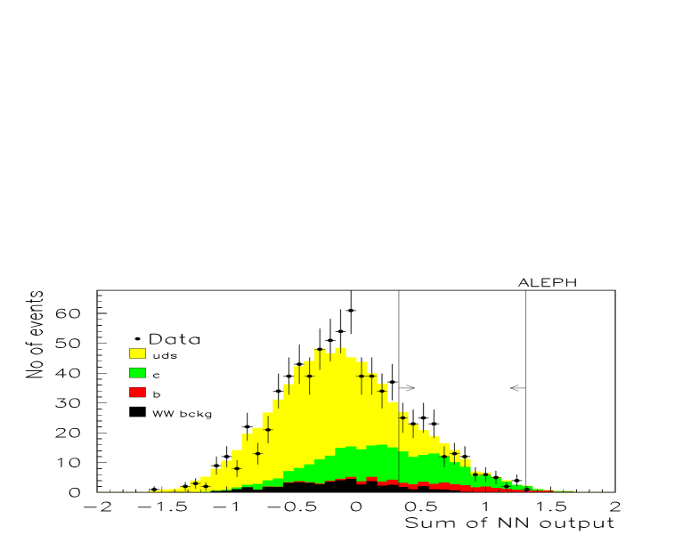
Figure 6: Distribution of the sum of the neural network outputs for hadronic events at 183 GeV centre-of-mass energy after hadronic selection and ${\mathrm{b}}\bar{\mathrm{b}}$  rejection. The lines indicate the chosen cuts.

To evaluate the systematic uncertainty introduced by a given selection variable, the ratio of distributions of this variable in data to Monte Carlo is determined. After smoothing to reduce statistical fluctuations, this ratio is then used to reweight individually ${\mathrm{b}}\bar{\mathrm{b}}$, ${\mathrm{c}}\bar{\mathrm{c}}$  and light quark event flavours in the Monte Carlo. The relative change in the resulting efficiency for each flavour is taken as its systematic uncertainty. A cross-check is performed by measuring $R_{\mathrm{c}}$ on the Z data taken in the same year; the measured value is consistent with the SM prediction. All contributions to the systematic uncertainty are given in Table 8.

Table 7: Selection efficiency for each flavour, and its expected fraction in the final event sample, assuming SM cross sections.

	Efficiency (%)	Fraction (%)
${\mathrm{u}}\bar{\mathrm{u}}$	$6.18\pm 0.25$	$14.8\pm 0.6$
${\mathrm{d}}\bar{\mathrm{d}}$	$6.66\pm 0.33$	$10.3\pm 0.5$
${\mathrm{s}}\bar{\mathrm{s}}$	$6.09\pm 0.31$	$9.7\pm 0.5$
${\mathrm{c}}\bar{\mathrm{c}}$	$22.07\pm 0.48$	$51.8\pm 0.8$
${\mathrm{b}}\bar{\mathrm{b}}$	$8.61\pm 0.37$	$13.4\pm 0.6$

Table 8: Contributions to the systematic uncertainty on the measured value of $R_{\mathrm{c}}$.

Description	Uncertainty
Luminosity	$\pm 0.001$
Efficiency of ${\mathrm{q}}\bar{\mathrm{q}}$ selection	$\pm 0.001$
Background in ${\mathrm{q}}\bar{\mathrm{q}}$ selection	$\pm 0.001$
Performance of ${\mathrm{b}}\bar{\mathrm{b}}$  rejection tag	$\mbox{}^{+0.012}_{-0.003}$
Performance of neural network	$\mbox{}^{+0.006}_{-0.010}$
MC statistics	$\pm 0.007$
Total	$\mbox{}^{+0.016}_{-0.013}$

In the data, 153 events are selected, of which 74.8 are estimated from the Monte Carlo simulation to be background. The value of $R_{\mathrm{c}}$ at $\sqrt{s}=183$ GeV, for $\sqrt{s^{\prime}/s}>0.9$ and $|{\cos\theta}|<0.95$, where $\theta$ is the polar angle of the c quark with respect to the beam axis, is found to be

$$R_{\mathrm{c}}=0.276\pm 0.041({\mathrm{s}tat})\ ^{+0.016}_{-0.013}({\mathrm{s}yst})-0.284\times(R_{\mathrm{u}ds}-0.584)-0.390\times(R_{\mathrm{b}}-0.171)~{},$$ (4)

where the dependence on a possible departure of the light quark or ${\mathrm{b}}\bar{\mathrm{b}}$ fractions from their SM expectations is explicitly given. The measured value of $R_{\mathrm{c}}$ is consistent with its SM expectation of 0.244 .

5.4 Measurement of $A_{\mathrm{F}B}^{\mathrm{q}}$ using Jet Charge

Constraints upon the forward-backward asymmetries $A_{\mathrm{F}B}^{\mathrm{q}}$ of ${\mathrm{q}}\bar{\mathrm{q}}$ events at $\sqrt{s}=183$ GeV are obtained using a jet charge technique. This is performed separately for b-enriched and b-depleted events, which allows the asymmetry in ${\mathrm{b}}\bar{\mathrm{b}}$ events to be well determined.

The analysis uses the hadronic events with $\sqrt{s^{\prime}/s}>0.9$, selected as described in Section 5.1. To ensure that the events are well contained in the tracking chambers, they are also required to satisfy $|{\cos\theta^{*}}|<0.9$. The events are then divided into two samples, according to whether they pass or fail the b lifetime tag of Section 5.2 (here used with looser cuts). This gives a 91% pure sample of ${\mathrm{b}}\bar{\mathrm{b}}$  events plus a sample of predominantly light/charm quark events.

After clustering all the events into two jets, the jet charge $Q_{\mathrm{j}et}$ of each jet is determined, where

$$Q_{\mathrm{j}et}=\left.{\displaystyle\sum_{i=1}^{\mathrm{N}_{track}}p_{\parallel i}^{\kappa}Q_{i}}\right/{\displaystyle\sum_{i=1}^{\mathrm{N}_{track}}p_{\parallel i}^{\kappa}}$$ (5)

and the sums extend over the charged tracks in the jet. The track momentum component parallel to the jet and its charge are $p_{\parallel i}$ and $Q_{i}$, respectively. The parameter $\kappa$ is set to 0.3, because this minimizes the uncertainty on the final result. The mean charge difference between the forward and backward jets $\mbox{$\langle Q_{\mathrm{F}B}\rangle$}=\langle Q_{\mathrm{j}et}^{\mathrm{F}}\rangle-\langle Q_{\mathrm{j}et}^{\mathrm{B}}\rangle$ is then formed. The first row of Table 9 shows the observed value of $\langle Q_{\mathrm{F}B}\rangle$ in the data.

Table 9: Comparison of $\langle Q_{\mathrm{F}B}\rangle$ in data with the prediction of Equation 6 using SM values of $\sigma_{\mathrm{q}}$ and $A_{\mathrm{F}B}^{\mathrm{q}}$. Also shown is the contribution to this prediction from signal and background events.

$\langle Q_{\mathrm{F}B}\rangle$	b tagged events	anti-b tagged events
Data	$-0.029\pm 0.018$	$0.022\pm 0.007$
Expectation in SM	$-0.052$	$0.014$
Contribution from signal	$-0.048$	$0.018$
Contribution from background	$-0.004$	$-0.003$

The expected value of $\langle Q_{\mathrm{F}B}\rangle$ depends on the ${\mathrm{q}}\bar{\mathrm{q}}$ cross sections $\sigma_{\mathrm{q}}$ and asymmetries $A_{\mathrm{F}B}^{\mathrm{q}}$. Defining $\epsilon_{i}$ as the selection efficiency for event type $i$, the prediction is

$$\mbox{$\langle Q_{\mathrm{F}B}\rangle$}=\frac{\displaystyle\sum_{\mathrm{q}}\sigma_{\mathrm{q}}\epsilon_{\mathrm{q}}\mbox{$A_{\mathrm{F}B}^{\mathrm{q}}$}\delta_{\mathrm{q}}D_{\mathrm{q}}+\sum_{\mathrm{x}}\sigma_{\mathrm{x}}\epsilon_{\mathrm{x}}{\mbox{$\langle Q_{\mathrm{F}B}\rangle$}}_{x}}{\displaystyle\sum_{\mathrm{q}}\sigma_{\mathrm{q}}\epsilon_{\mathrm{q}}+\sum_{\mathrm{x}}\sigma_{\mathrm{x}}\epsilon_{\mathrm{x}}}~{},$$ (6)

where the sums extend over the quark flavours q and the various background types x. The parameters $\delta_{\mathrm{q}}=\langle{Q_{\mathrm{j}et}^{\mathrm{q}}}\rangle-\langle{Q_{\mathrm{j}et}^{\mathrm{\bar{}}q}}\rangle$ give the mean charge separation between the jet containing the quark and that containing the antiquark. Table 10 shows the parameters $\delta_{\mathrm{q}}$ for each flavour. They are obtained from Monte Carlo simulation, but with additional corrections based upon a precise analysis at the Z peak [19]. The parameters $\delta_{q}$ vary only slowly with centre-of-mass energy so these corrections are still applicable at LEP2. The most important correction is that to $\delta_{c}$, which amounts to 26%. This is due to an inadequate simulation of charm hadron decay modes. However, even this only alters the predicted value of $\langle Q_{\mathrm{F}B}\rangle$ by about one half of the statistical error in the data. Systematic uncertainties on the $\delta_{q}$ can therefore at present be neglected. The parameters $D_{\mathrm{q}}$ ($\approx 0.98$) give the dilution in ${\mbox{$\langle Q_{\mathrm{F}B}\rangle$}}_{\mathrm{q}}=\mbox{$A_{\mathrm{F}B}^{\mathrm{q}}$}\delta_{\mathrm{q}}D_{\mathrm{q}}$ caused by the small angular dependence of the acceptance efficiency.

Table 10: Mean jet charge separations for each quark flavour.

$\delta_{\mathrm{u}}$	$\delta_{\mathrm{d}}$	$\delta_{\mathrm{s}}$	$\delta_{\mathrm{c}}$	$\delta_{\mathrm{b}}$
$0.205$	$-0.130$	$-0.153$	$0.155$	$-0.108$

Assuming SM values of $\sigma_{\mathrm{q}}$ and $A_{\mathrm{F}B}^{\mathrm{q}}$, the predicted values of $\langle Q_{\mathrm{F}B}\rangle$ are given in the second row of Table 9. They agree with those measured in the data, both for the b-enriched and the b-depleted samples. By comparing the measured value of $\langle Q_{\mathrm{F}B}\rangle$ in each of these two samples with the predictions of Equation 6, two independent constraint equations are obtained for the allowed values of $\sigma_{\mathrm{q}}$ and $A_{\mathrm{F}B}^{\mathrm{q}}$.

Providing that deviations from the SM are small, it is convenient to approximate each of these two constraints by a linear equation. These two linear equations will be used when placing limits on physics beyond the SM in Section 7.

If $\sigma_{\mathrm{q}}$ and $A_{\mathrm{F}B}^{\mathrm{q}}$ differ from their SM predictions by $\Delta\sigma_{\mathrm{q}}$ and $\Delta\mbox{$A_{\mathrm{F}B}^{\mathrm{q}}$}$, respectively, then a Taylor expansion of Equation 6 yields

$$\mbox{$\langle Q_{\mathrm{F}B}\rangle$}-{\mbox{$\langle Q_{\mathrm{F}B}\rangle$}}_{\mathrm{S}M}=\sum_{\mathrm{q}}\frac{\partial\mbox{$\langle Q_{\mathrm{F}B}\rangle$}}{\partial\sigma_{\mathrm{q}}}\Delta\sigma_{\mathrm{q}}+\frac{\partial\mbox{$\langle Q_{\mathrm{F}B}\rangle$}}{\partial\mbox{$A_{\mathrm{F}B}^{\mathrm{q}}$}}\Delta\mbox{$A_{\mathrm{F}B}^{\mathrm{q}}$}~{}.$$ (7)

Dividing this equation throughout by the estimated uncertainty on the measured value of $\langle Q_{\mathrm{F}B}\rangle$ in the data gives an equation of the form

$$\gamma=\sum_{\mathrm{q}}\alpha_{\mathrm{q}}\Delta\sigma_{\mathrm{q}}+\beta_{\mathrm{q}}\Delta\mbox{$A_{\mathrm{F}B}^{\mathrm{q}}$}~{}.$$ (8)

Here $\gamma$ is the difference between the measured value of $\langle Q_{\mathrm{F}B}\rangle$ and that expected in the SM, divided by the measurement uncertainty (such that $\gamma$ has an uncertainty of $\pm 1$). The coefficients $\alpha_{\mathrm{q}}$ and $\beta_{\mathrm{q}}$, defined by this equation, can be expressed in terms of $\epsilon_{i}$, $\delta_{\mathrm{q}}$, $D_{\mathrm{q}}$ and ${\mbox{$\langle Q_{\mathrm{F}B}\rangle$}}_{x}$. The values of $\gamma$, $\alpha_{\mathrm{q}}$ and $\beta_{\mathrm{q}}$ for the b-enriched and b-depleted event samples are given in Table 11. The uncertainties in $\alpha_{\mathrm{q}}$ and $\beta_{\mathrm{q}}$ can be neglected. The equation obtained from the b-enriched sample can be interpreted as a measurement of $A_{\mathrm{F}B}^{\mathrm{b}}$, since $\beta_{b}$ dominates the other coefficients. It gives a measured value of $\mbox{$A_{\mathrm{F}B}^{\mathrm{b}}$}=0.33\pm 0.19$, compared with the SM prediction of 0.57 .

Table 11: Coefficients of the linear constraint Equation 8 derived for the b-enriched and b-depleted data samples. The units of $\alpha$ are pb^-1.

Event Sample	$\gamma$	$\alpha_{u}$	$\alpha_{d}$	$\alpha_{s}$	$\alpha_{c}$	$\alpha_{b}$	$\beta_{u}$	$\beta_{d}$	$\beta_{s}$	$\beta_{c}$	$\beta_{b}$
$b$ tagged	$1.3\pm 1.0$	$0.0$	$0.0$	$0.0$	$0.0$	$-0.1$	$0.0$	$0.0$	$0.0$	$0.4$	$-5.4$
anti-$b$ tagged	$1.2\pm 1.0$	$0.7$	$-0.6$	$-0.7$	$0.5$	$-0.2$	$6.6$	$-2.7$	$-3.4$	$5.1$	$-1.1$

6 Leptonic Final States

6.1 The $\mathrm{e}^{+}e^{-}$ Channel

Electron pair events are selected by requiring the presence of two good tracks of opposite charge with a polar angle to the beam axis of $|{\cos\theta}|<0.9$. The sum of the momenta of the two tracks must exceed 30% of the centre-of-mass energy. The total energy associated with them in the ECAL must be at least 40% of the centre-of-mass energy. When calculating this energy, if one of the tracks passes near a crack in the ECAL, then the associated HCAL energy is included if it matches the track extrapolation within 25 mrad. Furthermore, the energy of bremsstrahlung photons is included when within cones of $20^{\circ}$ around each track.

Only the exclusive cross section is measured, so the requirement $\sqrt{s^{\prime}_{m}/s}>0.9$ is applied. The main background is due to ISR and this is reduced to a level of 10 – 12%, by requiring that the invariant mass of the ${\mathrm{e}}^{+}{\mathrm{e}}^{-}$ final state, determined from the measured track momenta, exceeds 80 GeV/$c^{2}$. The resulting invariant mass distribution is shown in Fig. 7. The discrepancy between data and Monte Carlo seen in this figure arises from an inaccurate simulation of the momentum resolution of tracks at small angles to the beam axis. As the cut applied on the electron pair invariant mass is very loose, this does not lead to a significant systematic uncertainty. The normalization of the radiative background is determined from a fit to Fig. 7, using the expected shapes of the signal and background. The statistical uncertainty on the fit result leads to the systematic uncertainty due to radiative background quoted in Table 12.

The selection efficiencies are determined from BHWIDE Monte Carlo samples at each energy point. They are given, together with the estimated background, in Table 2. The uncertainties on the efficiencies are estimated by varying the calorimeter energy scales as in Section 5.1.

The exclusive cross section is determined in two polar angle ranges: $-0.9<\cos\theta^{*}<0.9$ and $-0.9<\cos\theta^{*}<0.7$. It is dominated by $t$ channel photon exchange, particularly in the forward region. The cross section measurements are given in Table 3. The contributions to the systematic uncertainties on these measurements are given in Table 12. Uncertainties from possible bias in the polar angle measurement of tracks are negligible. They have been assessed by redetermining the cross section without using tracks having $|\cos\theta|>0.9$.

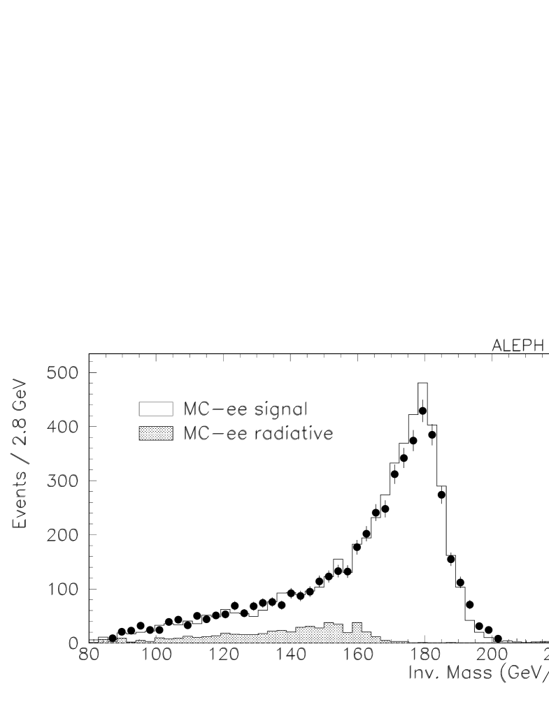
Figure 7: Electron pair invariant mass distribution at 183 GeV centre-of-mass energy. The data, which is shown by points, is compared with the Monte Carlo expectations for the signal and the radiative background.

Table 12: Contributions to the systematic uncertainties on the ${\mathrm{e}}^{+}{\mathrm{e}}^{-}$ exclusive cross section measurements, for both $\cos\theta^{*}$ intervals. All quoted values are in percent.

$\sqrt{s^{\prime}/s}$	$\cos\theta^{*}$ range	Description	$\mathrm{E}_{cm}$ (GeV)
cut			130	136	161	172	183
0.9	$-0.9<\cos\theta^{*}<0.9$	MC statistics	0.4	0.4	0.4	0.4	0.4
		Energy scale	1.7	1.6	1.4	1.6	1.6
		${\tau^{+}\tau^{-}}$	0.01	0.01	0.01	0.01	0.01
		Radiative background	0.9	1.0	0.9	1.0	0.9
		Luminosity	1.0	1.0	0.7	0.7	0.5
0.9	$-0.9<\cos\theta^{*}<0.7$	MC statistics	0.6	0.5	0.6	0.6	0.6
		Energy scale	1.4	1.3	1.2	1.2	1.1
		${\tau^{+}\tau^{-}}$	0.2	0.04	0.03	0.03	0.03
		Radiative background	1.3	1.6	1.3	1.4	1.3
		Luminosity	1.0	1.0	0.7	0.7	0.5

6.2 The $\mu^{+}\mu^{-}$ Channel

The muon pair selection requires events to contain two good, oppositely charged tracks with momenta exceeding 6 GeV/$c$ and angles to the beam axis of $|{\cos\theta}|<0.95$. The scalar sum of the momenta of the two tracks must exceed 60 GeV/$c$. The total number of good charged tracks in the events must be no more than eight. To limit the background from cosmic ray events, both tracks are required to originate near the primary vertex, and to have at least four associated ITC hits, which confirms that they were produced within a few nanoseconds of the LEP beam crossing.

Both tracks must be identified as muons, where muon identification is based either on the digital hit pattern associated with a track in the HCAL or on its energy deposition in the calorimeters:

• The track should fire at least 10 of the 23 drift tube planes in the HCAL. It should also fire at least half of the HCAL planes which the track is expected to cross (taking into account HCAL cracks), and furthermore should fire 3 or more of the outermost 10 planes of the HCAL. Alternatively, the track should have at least one associated hit in the muon chambers.

• The energy deposition must be consistent with that of a minimum ionizing particle, i.e., the sum of the energies associated with the track in the ECAL and HCAL should not exceed $60\%$ of the track momentum. Moreover, the sum of these energies and the track momentum should be smaller than $60\%$ of the centre-of-mass energy. To control a small misidentification background related to calorimeter cracks, tracks are also required to have at least one associated hit in the 10 outermost layers of the HCAL.

In the case of the exclusive selection, $\sqrt{s^{\prime}_{m}/s}>$0.9, it is also required that the muon pair invariant mass exceed 110 GeV/$c^{2}$, reducing background from radiative events by about 40%. The invariant mass distribution is shown in Fig. 8.

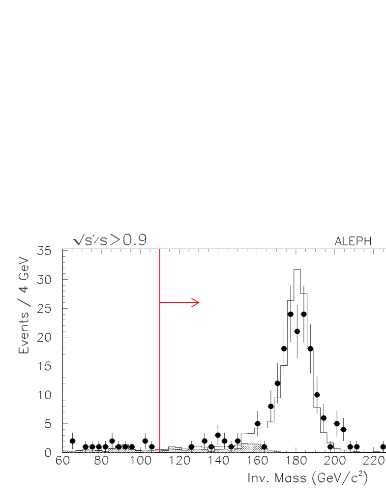
Figure 8: Distribution of the invariant mass of ${\mu^{+}\mu^{-}}$ events at $\sqrt{s}=183$ GeV, with $\sqrt{s^{\prime}_{m}/s}>$ 0.9. The data points are compared to the white histogram of Monte Carlo ${\mu^{+}\mu^{-}}$ events, normalized to the same integrated luminosity. The multi-radiative background is shown as the shaded histogram. The vertical line shows the cut used for the exclusive selection.

The efficiency of the kinematic selection cuts is estimated using KORALZ Monte Carlo events, whilst the muon identification efficiency is measured using muon pair events in data recorded at the Z peak in the same year. This efficiency is typically uncertain by about $\pm 1.6$% as a result of the limited number of Z events.

For the inclusive process, the main background contamination stems from $\gamma\gamma\rightarrow\mu^{+}\mu^{-}$. The systematic uncertainty associated with the normalization of this background is estimated by comparing data and Monte Carlo in the region of ${\mu^{+}\mu^{-}}$ mass below 50 GeV/$c^{2}$, which is shown in Fig. 9.

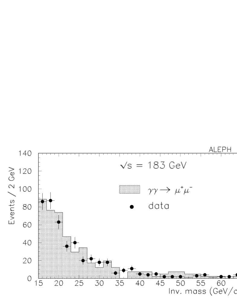
Figure 9: Distribution of the invariant mass of ${\mu^{+}\mu^{-}}$ events at 183 GeV centre-of-mass energy in the low mass region where the process $\gamma\gamma\rightarrow\mu^{+}\mu^{-}$ is dominant. The Monte Carlo prediction is indicated by the shaded histogram.

For the exclusive process, the main background comes from radiative events and is assessed using the mass region below $0.9\sqrt{s}$ of Fig. 8. Residual cosmic ray contamination is estimated by relaxing cuts on track impact parameters, and is found to be less than 0.5%.

Efficiencies and background levels are summarized in Table 2, and the cross section measurements are given in Table 3. The contributions to the systematic uncertainties on the cross sections are given in Table 13.

Table 13: Contributions to the systematic uncertainties on the muon pair cross section measurements, for all energies and for both inclusive and exclusive processes. All quoted values are in percent.

$\sqrt{s^{\prime}/s}$	Description	$\mathrm{E}_{cm}$ (GeV)
cut		130	136	161	172	183
0.1	MC statistics	0.4	0.4	0.4	0.4	0.4
	$\mu$ identification	2.0	2.0	1.9	2.0	1.9
	$\gamma\gamma\rightarrow\mu^{+}\mu^{-}$	0.0	0.0	1.0	1.0	0.7
	${\tau^{+}\tau^{-}}$	0.04	0.05	0.1	0.1	0.1
	$\mathrm{W}^{+}W^{-}$	—	—	0.05	0.2	0.3
	Luminosity	1.0	1.0	0.7	0.7	0.5
0.9	MC statistics	0.4	0.4	0.4	0.3	0.4
	$\mu$ identification	1.9	1.9	1.8	1.8	1.9
	${\tau^{+}\tau^{-}}$	0.00	0.00	0.02	0.1	0.1
	$\mathrm{W}^{+}W^{-}$	—	—	0.0	0.03	0.2
	Radiative background	0.5	0.5	0.6	0.8	0.6
	Luminosity	1.0	1.0	0.7	0.7	0.5

6.3 The $\tau^{+}\tau^{-}$ Channel

The tau pair selection begins by clustering events into jets, using the JADE algorithm with the clustering parameter $y_{\mathrm{c}ut}$ equal to 0.008 . Tau jet candidates must contain between one and eight charged tracks. Events with two tau jet candidates are selected, providing that the invariant mass of the two jets exceeds 25 GeV/$c^{2}$. This requirement removes a large part of the $\gamma\gamma$ background.

Following an approach already used for tau identification at LEP1 [20], each tau jet candidate is analysed and classified as a tau lepton decay into an electron, a muon, charged hadrons or charged hadrons plus one or more $\pi^{0}$. Both tau jets must be classified in this way. Events are required to have at least one tau jet candidate identified as a decay into a muon or into charged hadrons or charged hadrons plus $\pi^{0}$. To suppress background from $\gamma\gamma\rightarrow\mu^{+}\mu^{-}$ or ${\mu^{+}\mu^{-}}$, events with two jets classified as muonic tau decay are discarded.

For the exclusive selection, W pair events in which both W decay leptonically represent an important background. However, most of this background is rejected by requiring that the acoplanarity angle between the two taus be less than 250 mrad.

Estimated selection efficiencies and background levels are given in Table 2. A more detailed breakdown of the selection efficiencies for the various tau decay channels is given in Table 14. The main uncertainty on the selection efficiency arises from the energy scale of the calorimeters and is estimated as in Section 5.1. For the inclusive cross section the dominant background comes from $\gamma\gamma\rightarrow\tau^{+}\tau^{-}$. The systematic uncertainty associated with the normalization of this background is estimated from a comparison of data and Monte Carlo in the low visible mass range of selected tau pair events (15 GeV/$c^{2}$ $<M_{\mathrm{v}is}<$ 50 GeV/$c^{2}$). In the exclusive selection, the dominant background is Bhabha events, which sometimes pass the selection criteria if they enter cracks in the ECAL acceptance.

The cross section measurements are listed in Table 3. The contributions to the systematic uncertainties are given in Table 15.

Table 14: Percentage efficiency of the ${\tau^{+}\tau^{-}}$ selection for the various tau decay channels at a centre-of-mass energy of 183 GeV.

$\tau_{1}$ decay	/	$\tau_{2}$ decay	$\sqrt{{\rm s}^{\prime}{\rm/s}}\,>\,$0.1	$\sqrt{{\rm s}^{\prime}{\rm/s}}\,>\,$0.9
$\mu\nu_{\mu}\nu_{\tau}$	/	$\mu\nu_{\mu}\nu_{\tau}$	0.8 $\pm$ 0.5	1.1 $\pm$ 1.1
$\mu\nu_{\mu}\nu_{\tau}$	/	hadrons$\,\nu_{\tau}$	56.3 $\pm$ 1.8	77.1 $\pm$ 2.5
$\mu\nu_{\mu}\nu_{\tau}$	/	hadrons$\,\pi^{0}\,\nu_{\tau}$	61.7 $\pm$ 1.3	87.3 $\pm$ 1.5
$\mu\nu_{\mu}\nu_{\tau}$	/	e$\nu_{\mathrm{e}}\nu_{\tau}$	49.2 $\pm$ 2.1	74.9 $\pm$ 2.9
hadrons$\,\nu_{\tau}$	/	hadrons$\,\nu_{\tau}$	48.0 $\pm$ 2.2	67.5 $\pm$ 3.3
hadrons$\,\nu_{\tau}$	/	hadrons$\,\pi^{0}\,\nu_{\tau}$	53.6 $\pm$ 1.2	77.9 $\pm$ 1.6
hadrons$\,\nu_{\tau}$	/	e$\nu_{\mathrm{e}}\nu_{\tau}$	31.6 $\pm$ 1.7	50.2 $\pm$ 2.9
hadrons$\,\pi^{0}\,\nu_{\tau}$	/	hadrons$\,\pi^{0}\,\nu_{\tau}$	58.7 $\pm$ 1.2	79.9 $\pm$ 1.6
hadrons$\,\pi^{0}\,\nu_{\tau}$	/	e$\nu_{\mathrm{e}}\nu_{\tau}$	35.2 $\pm$ 1.3	48.5 $\pm$ 2.1
e$\nu_{\mathrm{e}}\nu_{\tau}$	/	e$\nu_{\mathrm{e}}\nu_{\tau}$	0.0	0.0

Table 15: Contributions to the systematic uncertainties on the ditau cross section measurements, for all energies and for both inclusive and exclusive processes. All quoted values are in percent.

$\sqrt{s^{\prime}/s}$	Description	$\mathrm{E}_{cm}$ (GeV)
cut		130	136	161	172	183
0.1	MC statistics	0.9	0.9	1.1	1.1	1.0
	Energy scale	1.6	1.7	1.6	1.6	1.5
	$\gamma\gamma\rightarrow\tau^{+}\tau^{-}$	0.5	0.6	0.7	1.2	0.5
	$\gamma\gamma\rightarrow\mu^{+}\mu^{-}$	0.8	0.9	0.8	0.9	0.1
	${\mathrm{q}}\bar{\mathrm{q}}$	0.4	0.4	0.1	0.3	0.3
	${\mathrm{e}}^{+}{\mathrm{e}}^{-}$	0.7	0.7	0.5	1.0	0.6
	$\mathrm{W}^{+}W^{-}$	—	—	—	0.4	0.7
	Luminosity	1.0	1.0	0.7	0.7	0.5
0.9	MC statistics	1.4	1.3	1.4	1.2	1.2
	Energy scale	2.0	2.0	2.2	2.1	2.3
	$\gamma\gamma\rightarrow\tau^{+}\tau^{-}$	0.5	0.8	0.6	1.0	0.4
	${\mathrm{q}}\bar{\mathrm{q}}$	0.4	0.6	0.7	0.3	0.3
	${\mathrm{e}}^{+}{\mathrm{e}}^{-}$	1.3	0.9	1.0	0.8	0.9
	${\mu^{+}\mu^{-}}$	0.1	0.1	0.1	0.1	0.1
	$\mathrm{W}^{+}W^{-}$	—	—	—	0.2	0.4
	Radiative background	1.0	1.4	2.7	0.5	0.7
	Luminosity	1.0	1.0	0.7	0.7	0.5

6.4 Measurement of the Lepton Asymmetries

Figures 10, 11 and 12 show the observed $\cos\theta^{*}$ distributions for electron, muon and tau pair events passing the exclusive selections at a centre-of-mass energy of 183 GeV.

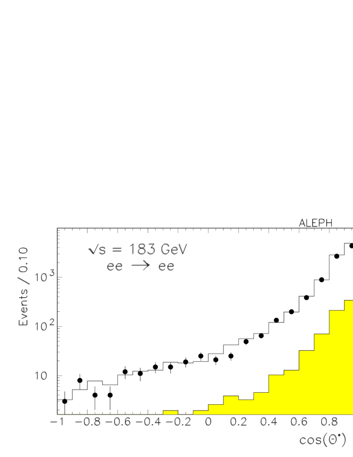
Figure 10: Distribution of $\cos\theta^{*}$ in Bhabha events at 183 GeV with $\sqrt{s^{\prime}_{m}/s}>0.9$. The data are represented by points, whilst the Monte Carlo expectation, normalized to the same integrated luminosity, is shown by the white histogram. The expected background is indicated by the shaded histogram.

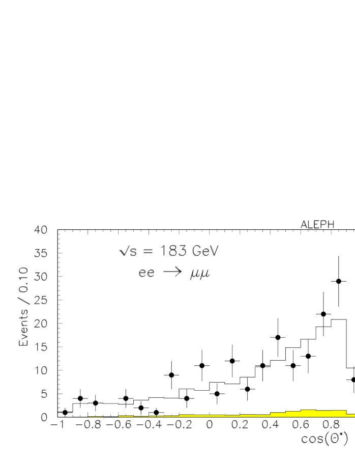
Figure 11: Distribution of $\cos\theta^{*}$ in ${\mu^{+}\mu^{-}}$ events at 183 GeV with $\sqrt{s^{\prime}_{m}/s}>0.9$. The data are represented by points, whilst the Monte Carlo expectation, normalized to the same integrated luminosity, is shown by the white histogram. The expected background is indicated by the shaded histogram.

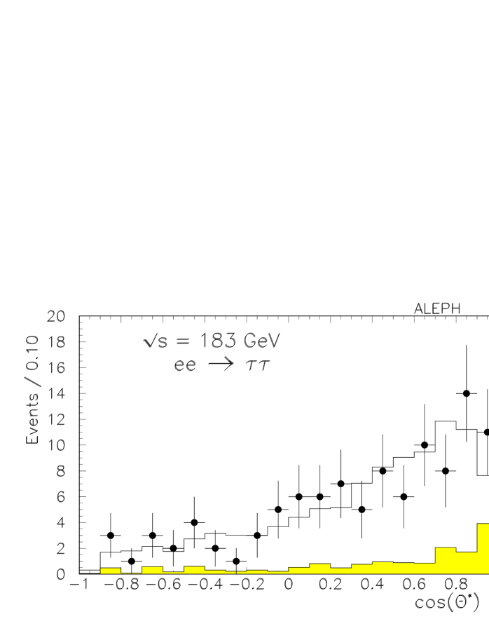
Figure 12: Distribution of $\cos\theta^{*}$ in ditau events at 183 GeV with $\sqrt{s^{\prime}_{m}/s}>0.9$. The data are represented by points, whilst the Monte Carlo expectation, normalized to the same integrated luminosity, is shown by the white histogram. The expected background is indicated by the shaded histogram.

As discussed in Section 2, the dilepton asymmetries are determined from the fraction of events in which the negatively charged lepton enters the forward/backward hemispheres with respect to the incoming electron. They are measured only for the exclusive process and defined in the range $|{\cos\theta}|<0.95$, where $\theta$ is the polar angle of the outgoing lepton. To ensure that the lepton charges are well measured, only events with $|{\cos\theta^{*}}|<0.9$ are used. Furthermore, only unambiguously charged events are kept, i.e., the product of the charge of the two leptons must be $-1$. This requirement removes about 0.5% of the muon pairs and 6% of the tau pairs. The remaining charge misidentification level is estimated using simulated events to be 0.002% for muon pairs and 0.05% for tau pairs. The asymmetries are corrected for backgrounds and acceptance, using the appropriate Monte Carlo samples. This includes the effect of extrapolating from $|{\cos\theta^{*}}|<0.9$ to $|{\cos\theta}|<0.95$.

The measured ${\mu^{+}\mu^{-}}$ and ${\tau^{+}\tau^{-}}$ asymmetries are shown in Table 16. For the Bhabha channel, rather than quoting an asymmetry, it is preferred to give the differential cross section with respect to $\theta^{*}$, because the reaction is dominated by $t$ channel photon exchange. This is given in Table 17.

A major contribution to the systematic uncertainties on the asymmetries is the background subtraction. The ditau channel is particularly sensitive to the Bhabha background since this is very peaked in the forward direction. For the tau pair asymmetry, this gives a correction of 1.3–3.8% for centre-of-mass energies of 130–183 GeV, respectively. The Monte Carlo statistical error on this correction enters as a part of the systematic uncertainty of the ditau asymmetry. Several other sources of systematic uncertainty are considered. The correction for event acceptance related to the extrapolation in polar angle introduces a significant uncertainty related to the finite Monte Carlo statistics. It also leads to a theoretical uncertainty due to ISR/FSR interference. This is assessed using ZFITTER. Systematic uncertainties from charge misidentification are negligible.

Table 16: Lepton forward-backward asymmetries with statistical and systematic uncertainties, calculated for $\sqrt{s^{\prime}/s}\,>\,$0.9 in the range $|{\cos\theta}|<0.95$.

$\mathrm{E}_{cm}$	Lepton	AFB	SM prediction
(GeV)	Type
130	$\mu^{+}\mu^{-}$	0.83 $\pm$ 0.08 $\pm$ 0.03	0.70
	$\tau^{+}\tau^{-}$	0.56 $\pm$ 0.12 $\pm$ 0.05	0.70
136	$\mu^{+}\mu^{-}$	0.63 $\pm$ 0.12 $\pm$ 0.03	0.68
	$\tau^{+}\tau^{-}$	0.65 $\pm$ 0.15 $\pm$ 0.04	0.68
161	$\mu^{+}\mu^{-}$	0.63 $\pm$ 0.11 $\pm$ 0.03	0.61
	$\tau^{+}\tau^{-}$	0.48 $\pm$ 0.14 $\pm$ 0.04	0.61
172	$\mu^{+}\mu^{-}$	0.72 $\pm$ 0.13 $\pm$ 0.04	0.59
	$\tau^{+}\tau^{-}$	0.44 $\pm$ 0.20 $\pm$ 0.04	0.59
183	$\mu^{+}\mu^{-}$	0.54 $\pm$ 0.06 $\pm$ 0.03	0.58
	$\tau^{+}\tau^{-}$	0.52 $\pm$ 0.08 $\pm$ 0.04	0.58

Table 17: Cross sections to produce electron pairs with $\sqrt{s^{\prime}/s}>0.9$ and $\cos\theta^{*}$ in the quoted ranges. The quoted uncertainties include statistical and systematic components.

$\mathrm{E}_{cm}$ (GeV)	$\cos\theta^{*}_{\mathrm{m}in},\cos\theta^{*}_{\mathrm{m}ax}$		$\sigma$ (pb)		SM prediction
130	$-0.9$,	$-0.7$	0.19$\,\;\pm\;\,$	0.34	0.37
	$-0.7$,	$-0.5$	1.41$\,\;\pm\;\,$	0.35	0.55
	$-0.5$,	$-0.3$	1.36$\,\;\pm\;\,$	0.45	1.09
	$-0.3$,	$-0.1$	1.23$\,\;\pm\;\,$	0.48	1.19
	$-0.1$,	$0.1$	2.60$\,\;\pm\;\,$	0.69	2.45
	$0.1$,	$0.3$	3.78$\,\;\pm\;\,$	0.83	3.82
	$0.3$,	$0.5$	8.88$\,\;\pm\;\,$	1.18	7.36
	$0.5$,	$0.7$	21.63$\,\;\pm\;\,$	2.12	22.20
	$0.7$,	$0.9$	149.61$\,\;\pm\;\,$	6.22	148.00
136	$-0.9$,	$-0.7$	0.73$\,\;\pm\;\,$	0.20	0.22
	$-0.7$,	$-0.5$	1.16$\,\;\pm\;\,$	0.36	0.62
	$-0.5$,	$-0.3$	0.54$\,\;\pm\;\,$	0.35	0.49
	$-0.3$,	$-0.1$	0.52$\,\;\pm\;\,$	0.41	0.89
	$-0.1$,	$0.1$	1.46$\,\;\pm\;\,$	0.62	2.09
	$0.1$,	$0.3$	2.09$\,\;\pm\;\,$	0.74	2.96
	$0.3$,	$0.5$	6.68$\,\;\pm\;\,$	1.08	6.13
	$0.5$,	$0.7$	16.58$\,\;\pm\;\,$	1.97	20.50
	$0.7$,	$0.9$	132.55$\,\;\pm\;\,$	5.85	133.00
161	$-0.9$,	$-0.7$	0.46$\,\;\pm\;\,$	0.21	0.37
	$-0.7$,	$-0.5$	0.88$\,\;\pm\;\,$	0.21	0.44
	$-0.5$,	$-0.3$	0.55$\,\;\pm\;\,$	0.28	0.79
	$-0.3$,	$-0.1$	0.39$\,\;\pm\;\,$	0.26	0.62
	$-0.1$,	$0.1$	1.24$\,\;\pm\;\,$	0.40	1.43
	$0.1$,	$0.3$	2.37$\,\;\pm\;\,$	0.47	2.07
	$0.3$,	$0.5$	5.35$\,\;\pm\;\,$	0.73	4.95
	$0.5$,	$0.7$	14.38$\,\;\pm\;\,$	1.27	14.10
	$0.7$,	$0.9$	93.76$\,\;\pm\;\,$	3.76	94.20
172	$-0.9$,	$-0.7$	0.32$\,\;\pm\;\,$	0.19	0.28
	$-0.7$,	$-0.5$	0.88$\,\;\pm\;\,$	0.19	0.34
	$-0.5$,	$-0.3$	0.66$\,\;\pm\;\,$	0.24	0.58
	$-0.3$,	$-0.1$	0.61$\,\;\pm\;\,$	0.23	0.44
	$-0.1$,	$0.1$	0.95$\,\;\pm\;\,$	0.36	1.23
	$0.1$,	$0.3$	1.80$\,\;\pm\;\,$	0.47	1.93
	$0.3$,	$0.5$	4.92$\,\;\pm\;\,$	0.71	4.24
	$0.5$,	$0.7$	13.07$\,\;\pm\;\,$	1.20	12.40
	$0.7$,	$0.9$	84.61$\,\;\pm\;\,$	3.51	81.10
183	$-0.9$,	$-0.7$	0.24$\,\;\pm\;\,$	0.07	0.21
	$-0.7$,	$-0.5$	0.29$\,\;\pm\;\,$	0.07	0.25
	$-0.5$,	$-0.3$	0.46$\,\;\pm\;\,$	0.10	0.51
	$-0.3$,	$-0.1$	0.71$\,\;\pm\;\,$	0.12	0.64
	$-0.1$,	$0.1$	0.83$\,\;\pm\;\,$	0.14	0.90
	$0.1$,	$0.3$	1.42$\,\;\pm\;\,$	0.20	1.83
	$0.3$,	$0.5$	3.90$\,\;\pm\;\,$	0.29	3.66
	$0.5$,	$0.7$	12.47$\,\;\pm\;\,$	0.56	11.10
	$0.7$,	$0.9$	71.90$\,\;\pm\;\,$	1.86	71.80

7 Interpretation in Terms of New Physics

7.1 Comparison with Standard Model Predictions

The measured cross sections and asymmetries from Tables 3 and 16 are plotted as a function of centre-of-mass energy in Figs. 13 and 14, respectively. The results are compared with SM predictions based on BHWIDE [7] for electron pair production and ZFITTER [21] for all other processes. The ZFITTER predictions are computed from the input values $m_{\mathrm{Z}}=91.1867$ GeV/$c^{2}$, $m_{\mathrm{t}}=174.1$ GeV/$c^{2}$, $m_{\mathrm{H}}=127.0$ GeV/$c^{2}$, $\alpha_{\mathrm{e}m}(M_{\mathrm{Z}})=1/128.896$ and $\alpha_{s}(M_{\mathrm{Z}})=0.120$. The exclusive cross sections and asymmetries are given in the restricted angular range for the outgoing fermion direction, $|{\cos\theta}|<0.95$. The inclusive cross sections correspond to the full angular range.

Figure 13: Measured cross sections for fermion pair production. The curves indicate the predictions obtained from BHWIDE for the Bhabha process and from ZFITTER for the other channels. (Some of the points are shifted slightly along the horizontal axis to prevent them overlapping).

Figure 14: Measured asymmetries for muon and tau pair production. The curves indicate the predictions obtained from ZFITTER. (Some of the points are shifted slightly along the horizontal axis to prevent them overlapping).

Because of the poor knowledge of the contribution of ISR/FSR interference, the ZFITTER predictions are assigned a systematic uncertainty equal to the difference in the predictions with and without interference. This amounts to 1.5% for the hadronic cross section and 2% for the ${\mu^{+}\mu^{-}}$, ${\tau^{+}\tau^{-}}$, ${\mathrm{b}}\bar{\mathrm{b}}$  and ${\mathrm{c}}\bar{\mathrm{c}}$  cross sections. These uncertainties would almost double if one attempted to extrapolate the results to the full angular range. The Bhabha cross section is assumed to be uncertain by 3%, based on a study of different event generators. These uncertainties are taken into account in the calculation of limits on physics beyond the SM given in the following sections.

The measured cross sections and asymmetries are consistent with SM predictions. Similar results have been published by the OPAL Collaboration [22]. The L3 Collaboration has published results covering centre-of-mass energies up to 172 GeV [23].

7.2 Limits on Four-Fermion Contact Interactions

Comparing the measured exclusive difermion cross sections and angular distributions with SM predictions allows one to place limits upon many possible extensions to the SM. One convenient parametrization of such effects is given by the addition of four-fermion contact interactions [24] to the known SM processes. Such contact interactions are characterized by a scale $\Lambda$, interpreted as the mass of a new heavy particle exchanged between the incoming and outgoing fermion pairs, and a coupling $g$ giving the strength of the interaction. Contact interactions are, for example, expected to occur if fermions are composite.

Following the notation of Ref. [25], the effective Lagrangian for the four-fermion contact interaction in the process $\mbox{${\mathrm{e}}^{+}{\mathrm{e}}^{-}$}\rightarrow\mbox{${\mathrm{f}}\bar{\mathrm{f}}$}$ is given by

$${\cal L}^{CI}=\frac{g^{2}\eta_{\mathrm{s}ign}}{(1+\delta)\mbox{$\Lambda$}^{2}}\sum_{i,j=L,R}\eta_{ij}[\bar{\mathrm{e}}_{i}\gamma^{\mu}{\mathrm{e}}_{i}][\bar{\mathrm{f}}_{j}\gamma_{\mu}{\mathrm{f}}_{j}]~{},$$ (9)

with $\delta=1$ if $\mathrm{f}=e$, or 0 otherwise. The fields ${\mathrm{e}}_{L,R}$ (${\mathrm{f}}_{L,R}$) are the left- and right-handed chirality projections of electron (fermion) spinors. The coefficients $\eta_{ij}$, which take a value between $-1$ and $+1$, indicate the relative contribution of the different chirality combinations to the Lagrangian. The sign of $\eta_{\mathrm{s}ign}$ determines whether the contact interaction interferes constructively or destructively with the SM amplitude. Several different models are considered in this analysis, corresponding to the choices of the $\eta_{\mathrm{s}ign}$ and $\eta_{ij}$ given in Table 18.

Table 18: Four-fermion interaction models.

Model	$\eta_{\mathrm{s}ign}$	$\eta_{\mathrm{LL}}$	$\eta_{\mathrm{RR}}$	$\eta_{\mathrm{LR}}$	$\eta_{\mathrm{RL}}$
LL±	$\pm 1$	1	0	0	0
RR±	$\pm 1$	0	1	0	0
VV±	$\pm 1$	1	1	1	1
AA±	$\pm 1$	1	1	$-1$	$-1$
LR±	$\pm 1$	0	0	1	0
RL±	$\pm 1$	0	0	0	1
LL+RR±	$\pm 1$	1	1	0	0
LR+RL±	$\pm 1$	0	0	1	1

In the presence of contact interactions the differential cross section for $\mbox{${\mathrm{e}}^{+}{\mathrm{e}}^{-}$}\rightarrow\mbox{${\mathrm{f}}\bar{\mathrm{f}}$}$ as a function of the polar angle $\theta$ of the outgoing fermion with respect to the $\mathrm{e}^{-}$ beam line can be written as

$$\frac{{d}\sigma}{{d}\cos\theta}=F_{\mathrm{S}M}(s,t)\left[1+\mbox{$\epsilon$}\frac{F_{\mathrm{I}F}^{\mathrm{B}orn}(s,t)}{F_{\mathrm{S}M}^{\mathrm{B}orn}(s,t)}+\mbox{$\epsilon$}^{2}\frac{F_{\mathrm{C}I}^{\mathrm{B}orn}(s,t)}{F_{\mathrm{S}M}^{\mathrm{B}orn}(s,t)}\right]$$ (10)

with $s$ and $t$ being the Mandelstam variables and $\mbox{$\epsilon$}=g^{2}\eta_{\mathrm{s}ign}/(4\pi\mbox{$\Lambda$}^{2})$. The SM cross section $F_{\mathrm{S}M}$ is computed as described in Section 7.1. The contributions to the cross section from the SM – contact interaction interference and from the pure contact interaction are denoted by $F_{\mathrm{I}F}^{\mathrm{B}orn}$ and $F_{\mathrm{C}I}^{\mathrm{B}orn}$, respectively. They are calculated in the improved Born approximation. The Born level formulae can be found in Ref. [25] and these are corrected for ISR according to Ref. [26]. Because no higher order calculations are available for the contact interactions, the ratios of these with the improved Born predictions for the SM cross sections are taken, to allow for a partial cancellation of higher order effects.

The predictions of Equation 10 are fitted to the data using a binned maximum likelihood method. For contact interactions affecting the dilepton channels, the likelihood function ${\cal L}$ is defined by

$${\cal L}=G(\alpha^{\mathrm{c}orr};1)\,\prod_{i}\,G(\alpha^{\mathrm{u}ncorr}_{i};1)\,\prod_{k}\,{\cal P}\left(\,N_{ik}^{\mathrm{d}ata},\left[N_{ik}^{\mathrm{p}red}(\mbox{$\epsilon$})+\alpha^{\mathrm{c}orr}\Delta n^{\mathrm{c}orr}_{ik}+\alpha^{\mathrm{u}ncorr}_{i}\Delta n^{\mathrm{u}ncorr}_{ik}\right]\,\right)~{}.$$ (11)

The indices $i$ and $k$ run over the centre-of-mass energy points and angular bins in $\cos\theta^{*}$, respectively. The function ${\cal P}$ gives the Poisson probability to observe $N_{ik}^{\mathrm{d}ata}$ events in the data if $N_{ik}^{\mathrm{p}red}$ are expected. The systematic uncertainties on the expected number of events which are (un)correlated between the centre-of-mass energy points are represented by ($\Delta n^{\mathrm{u}ncorr}$) $\Delta n^{\mathrm{c}orr}$, respectively. These uncertainties are taken into account using the parameters $\alpha^{\mathrm{c}orr}$ and $\alpha^{\mathrm{u}ncorr}_{i}$, which are constrained using Gaussian distributions $G$ with zero mean and unit standard deviation. These parameters are fitted together with the parameter $\epsilon$. The fit range in the angular distribution is chosen to be $|{\cos\theta^{*}}|<0.9$ for the Bhabha channel and $|{\cos\theta^{*}}|<0.95$ for the muon and tau pair channels.

For contact interactions affecting hadronic events, the sum over angular bins is dropped, and instead two additional terms are added to the likelihood function to take into account the constraints from the measurement of the jet charge asymmetries, given by Equation 8 and Table 11. The contact interaction can be assumed to couple to all quark flavours with equal strength. In this case, the jet charge asymmetry measurements improve the limits for some models by up to 70%, primarily because of their sensitivity to the relative cross sections of up- and down-type quarks. Alternatively, one can assume that contact interactions only affect the ${\mathrm{b}}\bar{\mathrm{b}}$ final state. Such interactions are strongly constrained using the measurement of $R_{\mathrm{b}}$ from Section 5.2 and the jet charge asymmetry in b-enriched events of Section 5.4.

Because of the quadratic dependence of the theoretical cross sections upon $\epsilon$, the likelihood function can have two maxima. The 68% confidence level limits ($\epsilon$⁺ and $\epsilon$^-) on $\epsilon$ are therefore estimated as follows:

$$\int_{-\infty}^{\mbox{$\epsilon$}^{-}}{\cal L}(\mbox{$\epsilon$}^{\prime})d\mbox{$\epsilon$}^{\prime}=\int_{\mbox{$\epsilon$}^{+}}^{\infty}{\cal L}(\mbox{$\epsilon$}^{\prime})d\mbox{$\epsilon$}^{\prime}=0.16\,\int_{-\infty}^{\infty}{\cal L}(\mbox{$\epsilon$}^{\prime})d\mbox{$\epsilon$}^{\prime}~{},$$ (12)

where for each value of $\mbox{$\epsilon$}^{\prime}$ the parameters $\alpha_{c}$ and $\alpha_{i}$ are chosen which maximize the likelihood. The results for contact interaction affecting leptonic final states are listed in Table 19. Table 20 gives the results obtained for contact interactions affecting both hadronic events and all difermion events.

Table 19: Limits on contact interactions coupling to dilepton final states. The 68% confidence level range is given for $\epsilon$ whilst the 95% confidence level limits are given for $\Lambda$. The results presented for ${\mathrm{l}}^{+}{\mathrm{l}}^{-}$  assume lepton universality.

Model	[$\mbox{$\epsilon$}^{-}$,$\mbox{$\epsilon$}^{+}$] (TeV-2)	$\Lambda^{-}$ (TeV)	$\Lambda^{+}$ (TeV)
$\mbox{${\mathrm{e}}^{+}{\mathrm{e}}^{-}$}\rightarrow\mbox{${\mathrm{e}}^{+}{\mathrm{e}}^{-}$}$
LL	[$-0.067,+0.021$]	3.2	3.5
RR	[$-0.067,+0.022$]	3.2	3.4
VV	[$-0.017,+0.003$]	6.4	8.0
AA	[$-0.018,+0.019$]	4.2	5.5
LR	[$-0.042,+0.015$]	4.0	4.2
LL+RR	[$-0.038,+0.009$]	4.2	5.0
LR+RL	[$-0.022,+0.006$]	5.5	6.5
$\mbox{${\mathrm{e}}^{+}{\mathrm{e}}^{-}$}\rightarrow\mbox{${\mu^{+}\mu^{-}}$}$
LL	[$-0.014,+0.040$]	4.7	4.0
RR	[$-0.016,+0.043$]	4.4	3.8
VV	[$-0.005,+0.016$]	7.7	6.3
AA	[$-0.009,+0.015$]	6.8	6.2
LR	[$-0.270,+0.025$]	1.8	3.8
LL+RR	[$-0.007,+0.022$]	6.6	5.4
LR+RL	[$-0.260,+0.019$]	1.9	5.1
$\mbox{${\mathrm{e}}^{+}{\mathrm{e}}^{-}$}\rightarrow\tau^{+}\tau^{-}$
LL	[$-0.039,+0.032$]	3.7	3.9
RR	[$-0.046,+0.034$]	3.4	3.7
VV	[$-0.012,+0.016$]	6.2	5.9
AA	[$-0.022,+0.013$]	5.2	5.6
LR	[$-0.275,+0.033$]	1.8	3.3
LL+RR	[$-0.020,+0.018$]	5.2	5.2
LR+RL	[$-0.265,+0.025$]	1.8	4.3
$\mbox{${\mathrm{e}}^{+}{\mathrm{e}}^{-}$}\rightarrow\mbox{${\mathrm{l}}^{+}{\mathrm{l}}^{-}$}$
LL	[$-0.014,+0.020$]	5.5	5.3
RR	[$-0.016,+0.021$]	5.3	5.1
VV	[$-0.005,+0.006$]	9.5	9.3
AA	[$-0.007,+0.010$]	8.0	7.5
LR	[$-0.023,+0.019$]	4.8	5.0
LL+RR	[$-0.008,+0.010$]	7.7	7.3
LR+RL	[$-0.011,+0.009$]	7.1	7.2

Table 20: Limits on contact interactions coupling to hadronic or to all difermion final states. The 68% confidence level range is given for $\epsilon$ whilst the 95% confidence level limits are given for $\Lambda$. The results presented for ${\mathrm{f}}\bar{\mathrm{f}}$  assume that the contact interaction couples to all the outgoing fermion types equally.

Model	[$\mbox{$\epsilon$}^{-}$,$\mbox{$\epsilon$}^{+}$] (TeV-2)	$\Lambda^{-}$ (TeV)	$\Lambda^{+}$ (TeV)
$\mbox{${\mathrm{e}}^{+}{\mathrm{e}}^{-}$}\rightarrow\mbox{${\mathrm{b}}\bar{\mathrm{b}}$}$
LL	[$-0.024,+0.013$]	4.9	5.6
RR	[$-0.232,-0.004$]	1.9	3.9
VV	[$-0.029,+0.007$]	4.6	6.5
AA	[$-0.016,+0.009$]	5.9	7.0
LR	[$-0.143,+0.054$]	2.3	3.0
RL	[$-0.028,+0.232$]	3.6	1.9
LL+RR	[$-0.018,+0.009$]	5.7	6.6
LR+RL	[$-0.036,+0.101$]	3.6	2.8
$\mbox{${\mathrm{e}}^{+}{\mathrm{e}}^{-}$}\rightarrow\mbox{${\mathrm{q}}\bar{\mathrm{q}}$}$
LL	[$-0.008,+0.022$]	6.2	5.4
RR	[$-0.025,+0.036$]	4.4	3.9
VV	[$-0.010,+0.013$]	7.1	6.4
AA	[$-0.004,+0.013$]	7.9	7.2
LR	[$-0.055,+0.079$]	3.3	3.0
RL	[$-0.045,+0.076$]	4.0	2.4
LL+RR	[$-0.007,+0.014$]	7.4	6.7
LR+RL	[$-0.029,+0.099$]	4.5	2.9
$\mbox{${\mathrm{e}}^{+}{\mathrm{e}}^{-}$}\rightarrow\mbox{${\mathrm{f}}\bar{\mathrm{f}}$}$
LL	[$-0.006,+0.016$]	7.2	6.2
RR	[$-0.013,+0.019$]	5.8	5.4
VV	[$-0.005,+0.005$]	10.1	9.8
AA	[$-0.003,+0.009$]	9.8	8.4
LR	[$-0.024,+0.020$]	4.8	4.9
RL	[$-0.029,+0.006$]	4.9	5.7
LL+RR	[$-0.004,+0.009$]	9.2	8.1
LR+RL	[$-0.014,+0.006$]	6.8	7.6

Although all the physics content is described by the well-defined parameter $\epsilon$, it is conventional to extract limits on the energy scale $\Lambda$, assuming $g^{2}=4\pi$. The $95\%$ confidence level limits $\mbox{$\epsilon$}_{95}^{\pm}$ are computed according to

$$\int_{0}^{\mbox{$\epsilon$}_{95}^{+}}{\cal L}(\mbox{$\epsilon$}^{\prime})d\mbox{$\epsilon$}^{\prime}=0.95\,\int_{0}^{\infty}{\cal L}(\mbox{$\epsilon$}^{\prime})d\mbox{$\epsilon$}^{\prime}~{},\qquad\int_{\mbox{$\epsilon$}_{95}^{-}}^{0}{\cal L}(\mbox{$\epsilon$}^{\prime})d\mbox{$\epsilon$}^{\prime}=0.95\,\int_{-\infty}^{0}{\cal L}(\mbox{$\epsilon$}^{\prime})d\mbox{$\epsilon$}^{\prime}~{},$$ (13)

which are then used to obtain

$$\mbox{$\Lambda$}^{\pm}=1\left/\sqrt{|\mbox{$\epsilon$}_{95}^{\pm}|}\right.~{}.$$ (14)

Limits on the energy scale are listed in Tables 19 and 20. One can drop the assumption $g^{2}=4\pi$, in which case these results become limits on $\sqrt{4\pi}\mbox{$\Lambda$}/g$.

These results are competitive with previous analyses of contact interactions already performed at LEP [22, 27], at the Tevatron [28] and at HERA [29]. However, models of ${\mathrm{e}}^{+}{\mathrm{e}}^{-}$${\mathrm{u}}\bar{\mathrm{u}}$ and ${\mathrm{e}}^{+}{\mathrm{e}}^{-}$${\mathrm{d}}\bar{\mathrm{d}}$ contact interactions which violate parity (LL, RR, LR and RL) are already severely constrained by atomic physics parity violation experiments, which quote limits of the order of $15$ TeV [30]. The LEP limits for the fully leptonic couplings or those involving b quarks are of particular interest since they are inaccessible at $\mathrm{p}\bar{p}$ or $\mathrm{e}p$ colliders.

7.3 Limits on R-parity Violating Sneutrinos

Supersymmetric theories with R-parity violation have terms in the Lagrangian of the form $\lambda_{ijk}{\mathrm{L}}_{i}{\mathrm{L}}_{j}\bar{\mathrm{E}}_{k}$, where $\mathrm{L}$ denotes a lepton doublet superfield and $\bar{\mathrm{E}}$ denotes a lepton singlet superfield. The parameter $\lambda$ is a Yukawa coupling, and $i$, $j$, $k=1$, 2, 3 are generation indices. The $\lambda_{ijk}$, which for the purposes of this analysis are assumed to be real, are non-vanishing only for $i<j$. These terms allow for single production of sleptons at ${\mathrm{e}}^{+}{\mathrm{e}}^{-}$ collider experiments.

At LEP, dilepton production cross sections could then differ from their SM expectations as a result of the exchange of R-parity violating sneutrinos in the $s$ or $t$ channels [31]. Table 21 shows the most interesting possibilities. Those involving $s$ channel sneutrino exchange lead to a resonance. For the results presented here, this resonance is assumed to have a width of 1 GeV/$c^{2}$, which can occur if the sneutrino also has R-parity conserving decay modes [31]. For a sneutrino only having the R-parity violating decay mode into lepton pairs, the width would be much less than this, leading to slightly better limits.

Table 21: For each dilepton channel, the table shows the coupling amplitude, the sneutrino type exchanged, and an indication of whether the exchange occurs in the $s$ or $t$ channel.

$\lambda^{2}$	${\mathrm{e}}^{+}{\mathrm{e}}^{-}$	$\mu^{+}\mu^{-}$	$\tau^{+}\tau^{-}$
$\lambda_{121}^{2}$	$\tilde{\nu}_{\mu}$ (s,t)	$\tilde{\nu}_{e}$ (t)	—
$\lambda_{131}^{2}$	$\tilde{\nu}_{\tau}$ (s,t)	—	$\tilde{\nu}_{e}$ (t)
$\lambda_{121}\lambda_{233}$	—	—	$\tilde{\nu}_{\mu}$ (s)
$\lambda_{131}\lambda_{232}$	—	$\tilde{\nu}_{\tau}$ (s)	—

Direct searches for R-parity violating sneutrinos at LEP have led to lower limits on their masses of 72 GeV/$c^{2}$ for $\tilde{\nu}_{e}$ and 49 GeV/$c^{2}$ for $\tilde{\nu}_{\mu}$ and $\tilde{\nu}_{\tau}$ [32]. Indirect limits based upon lepton universality and leptonic tau decays imply that the couplings in Table 21 must approximately satisfy $\lambda<0.1(m_{\tilde{l}_{R}}/200)$ GeV/$c^{2}$, where $m_{\tilde{l}_{R}}$ is the mass of the appropriate right-handed charged slepton [31]. These limits can be improved using the dilepton cross section and asymmetry data presented in this paper.

Limits on the couplings are obtained by comparing the measured dilepton differential cross sections with respect to the polar angle with the theoretical cross sections in reference [31]. The likelihood function used in the fit and the corrections for ISR, etc. follow the procedure of Section 7.2. The fit is performed in terms of the parameter $\lambda^{2}$. Since the likelihood function can have two minima, limits are again determined by integrating the likelihood function with respect to $\lambda^{2}$. A one-sided limit is used when $\lambda^{2}$ is positive definite, which occurs when $\lambda^{2}=\lambda_{121}^{2}$ or $\lambda_{131}^{2}$, but not when $\lambda^{2}=\lambda_{121}\lambda_{233}$ or $\lambda_{131}\lambda_{232}$.

Figures 15, 16 and 17 show the results for those processes involving sneutrino exchange in the $s$ channel. Similar results have been obtained by the OPAL Collaboration [22] and for $\tilde{\nu}_{\tau}$ by the L3 Collaboration [33].

Limits on $\lambda_{121}$ and $\lambda_{131}$ from $t$ channel exchange of $\tilde{\nu}_{e}$ in muon and tau pair production, respectively, give much weaker limits. These rise from $|\lambda_{1j1}|<0.5$ at $\tilde{\nu}_{e}=$ 100 GeV/$c^{2}$ to $|\lambda_{1j1}|<0.9$ at $\tilde{\nu}_{e}=$ 300 GeV/$c^{2}$.

Figure 15: 95% confidence level upper limits, obtained from the Bhabha cross sections, on $|\lambda_{121}|$ versus the assumed $\tilde{\nu}_{\mu}$ mass and on $|\lambda_{131}|$ versus the assumed $\tilde{\nu}_{\tau}$ mass.

Figure 16: 95% confidence level upper limits, obtained from the ${\mu^{+}\mu^{-}}$ cross sections, on $\sqrt{|\lambda_{131}\lambda_{232}|}$ versus the assumed $\tilde{\nu}_{\tau}$ mass.

Figure 17: 95% confidence level upper limits, obtained from the ditau cross sections, on $\sqrt{|\lambda_{121}\lambda_{233}|}$ versus the assumed $\tilde{\nu}_{\mu}$ mass.

7.4 Limits on Leptoquarks and R-Parity Violating Squarks

At LEP, the $t$ channel exchange of a leptoquark can modify the ${\mathrm{q}}\bar{\mathrm{q}}$ cross section and jet charge asymmetry, as described by the Born level equations given in Ref. [34]. A comparison of the measurements with these equations allows upper limits to be set on the leptoquark’s couplings $g$ as a function of its mass $M_{\mathrm{L}Q}$, using the same fit technique and corrections for ISR, etc. as employed in Section 7.2. Although the leptoquark $t$ channel exchange alters the angular distribution of the outgoing ${\mathrm{q}}\bar{\mathrm{q}}$ system, this has negligible effect on the ${\mathrm{q}}\bar{\mathrm{q}}$ selection efficiency. Limits are obtained for each possible leptoquark species. The allowed species can be classified according to their spin, weak isospin $I$ and hypercharge. Scalar and vector leptoquarks are denoted by symbols ${\mathrm{S}}_{I}$ and ${\mathrm{V}}_{I}$ respectively, and isomultiplets with different hypercharges are distinguished by a tilde. An indication “(L)” or “(R)” after the name indicates if the leptoquark couples to left- or right-handed leptons. Where both chirality couplings are possible, limits are set for the two cases independently, assuming that left- and right-handed couplings are not present simultaneously. It is also assumed that leptoquarks within a given isomultiplet are mass degenerate [34].

The $\mathrm{\tilde{}}S_{\mbox{$\scriptscriptstyle\frac{1}{2}$}}~{}(L)$ and $\mathrm{S}_{0}~{}(L)$ leptoquarks are equivalent to up-type anti-squarks and down-type squarks, respectively, in supersymmetric theories with an R-parity breaking term $\lambda^{\prime}_{1jk}{\mathrm{L}}_{1}{\mathrm{Q}}_{j}\bar{\mathrm{D}}_{k}$ $(j,k=1,2,3)$. Limits in terms of the leptoquark coupling are then exactly equivalent to limits in terms of $\lambda^{\prime}_{1jk}$.

Table 22 gives for each leptoquark type, the 95% confidence level lower limits on its mass $M_{\mathrm{L}Q}$, assuming that it has a coupling strength equal to the electromagnetic coupling $g=e$. The limits are given separately, assuming that (i) the leptoquark couples to only $1^{\mathrm{s}t}$ or only $2^{\mathrm{n}d}$ generation quarks, or (ii) to only $3^{\mathrm{r}d}$ generation quarks. The former limits are derived using the measured hadronic cross section and jet charge asymmetries, whilst the latter uses the ${\mathrm{b}}\bar{\mathrm{b}}$ cross section and jet charge asymmetries. For $g\not=e$, the mass limit scales approximately in proportion to the coupling if it exceeds about 200 GeV/$c^{2}$. (This is the contact term limit.)

Table 22: 95% confidence level lower limits on the leptoquark mass for each species. Limits are given separately according to the quark generation to which the leptoquark is assumed to couple. A dash indicates that no limit can be set and “N.A.” denotes leptoquarks coupling only to top quarks and hence not visible at LEP.

Quark	Limit on scalar leptoquark mass (GeV/$c^{2}$)
Generation	$\mathrm{S}_{0}~{}(L)$	$\mathrm{S}_{0}~{}(R)$	$\mathrm{\tilde{}}S_{0}~{}(R)$	$\mathrm{S}_{1}~{}(L)$	$\mathrm{S}_{\mbox{$\scriptscriptstyle\frac{1}{2}$}}~{}(R)$	$\mathrm{S}_{\mbox{$\scriptscriptstyle\frac{1}{2}$}}~{}(L)$	$\mathrm{\tilde{}}S_{\mbox{$\scriptscriptstyle\frac{1}{2}$}}~{}(L)$
$1^{\mathrm{s}t}$ or $2^{\mathrm{n}d}$	200	—	70	240	—	20	—
$3^{\mathrm{r}d}$	N.A.	N.A.	180	450	—	N.A.	50
Quark	Limit on vector leptoquark mass (GeV/$c^{2}$)
Generation	$\mathrm{V}_{\mbox{$\scriptscriptstyle\frac{1}{2}$}}~{}(R)$	$\mathrm{V}_{\mbox{$\scriptscriptstyle\frac{1}{2}$}}~{}(L)$	$\mathrm{\tilde{}}V_{\mbox{$\scriptscriptstyle\frac{1}{2}$}}~{}(L)$	$\mathrm{V}_{0}~{}(L)$	$\mathrm{V}_{0}~{}(R)$	$\mathrm{\tilde{}}V_{0}~{}(R)$	$\mathrm{V}_{1}~{}(L)$
$1^{\mathrm{s}t}$ or $2^{\mathrm{n}d}$	150	130	90	340	120	280	470
$3^{\mathrm{r}d}$	260	160	N.A.	400	140	N.A.	400

Similar limits have been obtained by OPAL and L3 [22, 27]. Limits from the Tevatron [35, 36] depend upon the assumed branching ratio of the charged leptonic decay mode. However, if this is 100%, then the Tevatron excludes leptoquark masses below $\sim$ 225 GeV/$c^{2}$. Other experiments can place limits on leptoquarks which couple to first generation quarks. In particular, low energy data such as atomic parity violation and rare decays give very stringent limits, usually as a function of the ratio $g/M_{\mathrm{L}Q}$. If $g=e$, they imply a lower limit on the leptoquark mass in the range 430–1500 GeV/$c^{2}$ [37], depending on the leptoquark species. Preliminary results from HERA [38] exclude scalar leptoquarks with masses below $\approx 250$ GeV/$c^{2}$ if $g=e$.

7.5 Limits on Extra Z Bosons

To unify the strong and electroweak interactions, Grand Unification Theories (GUT) extend the SM gauge group to a group of higher rank, predicting therefore the presence of at least one extra neutral gauge boson $\mathrm{Z}^{\prime}$. The theories which are considered in this section are the $E_{6}$ [39] and the Left-Right (LR) models [39]. In the $E_{6}$ model, the unification group $E_{6}$ can break into the SM $SU_{C}(3)\otimes SU_{L}(2)\otimes U_{Y}(1)$ in different ways. Each symmetry breaking pattern leads to the presence of at least one extra U(1) symmetry and therefore one extra gauge boson. This is characterized by a parameter $\theta_{E_{6}}$ ($-\pi/2\leq$ $\theta_{E_{6}}$$\leq\pi/2$) which entirely defines its couplings to conventional fermions. Contributions from exotic particles predicted by $E_{6}$ or supersymmetric particles are ignored in this analysis. Four models derived from $E_{6}$ are studied here, the $E_{6}(\chi)$, $E_{6}(\psi)$, $E_{6}(\eta)$ and $E_{6}(I)$ defined by $\theta_{E_{6}}$$=0$, $\pi/2$, $-\arctan{\sqrt{5/3}}$ and $\arctan{\sqrt{3/5}}$, respectively [39]. In the LR model, the SM group is extended to $SU_{C}(3)\otimes SU_{L}(2)\otimes SU_{R}(2)\otimes U_{B-L}(1)$, where B and L are the baryon and lepton number, respectively. The SM $U_{Y}(1)$ symmetry is recovered by a linear combination of the generator of $U_{B-L}(1)$ and the third component of $SU_{R}(2)$. This model, which can arise from symmetry breaking of the GUT group SO(10), leads to the presence of one extra neutral gauge boson. Contributions from the extra ${\mathrm{W}}_{R}$ of $SU(2)_{R}$ are neglected in this analysis. Couplings to conventional fermions depend only on one parameter $\alpha_{LR}$, where $\sqrt{2/3}\leq\alpha_{LR}\leq\sqrt{(1-2\sin^{2}{\theta}_{W})/\sin^{2}{\theta}_{W}}$, which is function of the coupling constants $g_{L,R}$ of $SU_{L,R}(2)$ and $\sin^{2}{\theta}_{W}$. Only the Left-Right Symmetric Model (LRS) will be studied here, which has $g_{L}=g_{R}$, implying that if $\sin^{2}{\theta}_{W}=0.23$ then $\mbox{$\alpha_{LR}$}=1.53$ .

Outside the context of GUT, a limit is derived on the mass of the non-gauge-invariant sequential SM (SSM) $\mathrm{Z}^{\prime}$ boson, having the same couplings as the SM Z, but with a higher mass. Limits are also placed upon the axial and vector couplings of an arbitrary $\mathrm{Z}^{\prime}$ as a function of its mass.

In all the models mentioned above, the symmetry eigenstate $\mathrm{Z}^{\prime 0}$ of the extra U(1) or $SU_{R}(2)$ can mix with the symmetry eigenstate $\mathrm{Z}^{0}$ of $SU_{L}(2)\otimes U_{Y}(1)$ with a mixing angle $\theta_{\mathrm{m}ix}$. In such a case, the Z resonance observed at LEP I must be identified as one of the mass eigenstates of the $\mathrm{Z}^{\prime 0}$–$\mathrm{Z}^{0}$ system while the second mass eigenstate $\mathrm{Z}^{\prime}$ of mass $m_{\mathrm{Z}^{\prime}}$ is a free parameter [40, 41].

To obtain the 95% confidence level exclusion limits on the various free parameters, least squares fits are performed using the set of ALEPH measurements given in Table 23, taking into account the correlations between them. The LEP1 measurements are taken from Ref. [42], whilst the LEP2 measurements are presented in Tables 3, 6 and 16.

Table 23: Set of observables used in the $\mathrm{Z}^{\prime}$ analyses and the corresponding SM $\chi^{2}$ values per degree of freedom.

	Observables	$\chi^{2}_{\mathrm{S}M}$/NDF.
LEP1	$\sigma^{\mathrm{l}^{+}l^{-}}$, $A^{\mathrm{l}^{+}l^{-}}_{FB}$, $\sigma^{{\mathrm{q}}\bar{\mathrm{q}}}$, $l=\mu,\tau$	130.9/120
LEP2	$\sigma^{\mathrm{l}^{+}l^{-}}$, $A^{\mathrm{l}^{+}l^{-}}_{FB}$, $\sigma^{{\mathrm{q}}\bar{\mathrm{q}}}$, $R_{\mathrm{b}}$	19.4/29
130–183 GeV	$l=\mu,\tau$, $\sqrt{s^{\prime}/s}>0.9$, $|{\cos\theta}|<0.95$

Theoretical predictions for difermion cross sections and asymmetries are obtained from the program ZEFIT 5.0 [41], which is an extension of ZFITTER 5.0 [21] including the one extra neutral gauge boson of the $E_{6}$, LR or SSM models. Theoretical uncertainties on the SM predictions are taken into account as described in Section 7.1. For all models, the minimum $\chi^{2}$ is found to occur when no $\mathrm{Z}^{\prime}$ boson is present.

For the five models $E_{6}(\chi)$, $E_{6}(\psi)$, $E_{6}(\eta)$, $E_{6}(I)$ and LRS, Fig. 18 shows the 95% confidence level limits obtained in the plane of $\mathrm{Z}^{\prime}$ mass versus mixing angle $\theta_{\mathrm{m}ix}$. Both parameters are treated as independent, so these limits correspond to a $\chi^{2}$ increase of 5.99 . The LEP1 data mainly constrain the mixing angle, whilst the LEP2 data mainly constrain the $\mathrm{Z}^{\prime}$ mass at small mixing angles.

Alternatively, assuming $\mbox{$\theta_{\mathrm{m}ix}$}=0$, lower limits on the $\mathrm{Z}^{\prime}$ mass can be obtained using a one-sided, one-parameter fit ($\Delta\chi^{2}=2.71$). The resulting limits are given in Table 24, where they are compared with those from direct $\mathrm{Z}^{\prime}$ searches performed by the CDF Collaboration [43]. This table also gives the mass limit for the SSM $\mathrm{Z}^{\prime}$, which is superior to the limit from CDF.

Table 24: Comparison of 95% confidence level lower limits on $m_{\mathrm{Z}^{\prime}}$ (GeV/$c^{2}$) from one parameter electroweak fits (ALEPH) and direct searches (CDF) for $\mbox{$\theta_{\mathrm{m}ix}$}=0$.

Model	ALEPH	CDF direct
$E_{6}(\chi)$	533	595
$E_{6}(\psi)$	294	590
$E_{6}(\eta)$	329	620
$E_{6}(I)$	472	565
LRS	436	630
Sequential SM	898	690

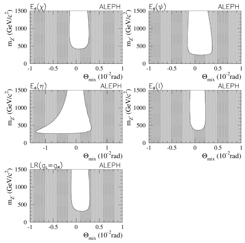
Figure 18: 95% confidence level limits in the $m_{\mathrm{Z}^{\prime}}$ vs. $\theta_{\mathrm{m}ix}$ plane for the $E_{6}(\chi)$, $E_{6}(\psi)$, $E_{6}(\eta)$, $E_{6}(I)$ and LRS models. The shaded regions are excluded.

Limits can also be placed on the vector and axial couplings of an arbitrary $\mathrm{Z}^{\prime}$, as a function of its mass. To simplify, such limits will only be given here for the leptonic couplings (assuming lepton universality) and also only for the case $\mbox{$\theta_{\mathrm{m}ix}$}=0$. Limits are placed on the two couplings simultaneously ($\Delta\chi^{2}=5.99$). The excluded region is found to be approximately rectangular in shape and its size is given as a function of $\mathrm{Z}^{\prime}$ mass in Table 25.

Table 25: 95% confidence level limits on the axial $g_{a}^{\prime}$ and vector $g_{v}^{\prime}$ couplings of a $\mathrm{Z}^{\prime}$ boson of mass $m_{\mathrm{Z}^{\prime}}$ to a lepton pair.

$m_{\mathrm{Z}^{\prime}}$ (GeV/$c^{2}$)	$|g_{a}^{\prime}|$	$|g_{v}^{\prime}|$
300	$\leq 0.36$	$\leq 0.28$
600	$\leq 0.81$	$\leq 0.64$
1000	$\leq 1.39$	$\leq 1.11$

8 Conclusions

Measurements of the hadronic and leptonic cross sections and asymmetries at $\sqrt{s}=\mbox{130--183}$ GeV have been presented. The ratios of the ${\mathrm{b}}\bar{\mathrm{b}}$ to ${\mathrm{q}}\bar{\mathrm{q}}$  production cross sections at $\sqrt{s}=130$–183 GeV and of the ${\mathrm{c}}\bar{\mathrm{c}}$ to ${\mathrm{q}}\bar{\mathrm{q}}$  production cross sections at $\sqrt{s}=183$ GeV have been shown, as well as jet charge asymmetries. The results agree with the predictions of the Standard Model and allow limits to be placed on four-fermion contact interactions, R-parity violating sneutrinos and squarks, leptoquarks and $\mathrm{Z}^{\prime}$ bosons. The limits on the energy scale $\Lambda$ of ${\mathrm{e}}^{+}{\mathrm{e}}^{-}$${\mathrm{f}}\bar{\mathrm{f}}$ contact interactions are typically in the range from 2–10 TeV. Those for ${\mathrm{e}}^{+}{\mathrm{e}}^{-}$${\mathrm{l}}^{+}{\mathrm{l}}^{-}$ and ${\mathrm{e}}^{+}{\mathrm{e}}^{-}$${\mathrm{b}}\bar{\mathrm{b}}$ interactions are of particular interest, since they are inaccessible at colliders using proton beams. The new ALEPH limits on R-parity violating sneutrinos reach masses of a few hundred GeV/$c^{2}$ for large values of their Yukawa couplings.

References

- [1] ALEPH Collaboration, “ALEPH: A detector for annihilations at LEP”, Nucl. Instrum. Methods A294 (1990) 121.
- [2] ALEPH Collaboration, “Performance of the ALEPH detector at LEP”, Nucl. Instrum. Methods A360 (1995) 481.
- [3] D. Creanza et al., “The new ALEPH silicon vertex detector”, Nucl. Instrum. Methods A409 (1998) 157.
- [4] ALEPH Collaboration, “Measurement of the absolute luminosity with the ALEPH detector”, Z. Phys. C53 (1992) 375.
- [5] A. Arbuzov et al., “The present theoretical error on the Bhabha scattering cross section in the luminosity region at LEP”, Phys. Lett. B383 (1996) 238.
- [6] S. Jadach et al., “Upgrade of the Monte Carlo program BHLUMI for Bhabha scattering at low angles to version 4.04”, Comp. Phys. Commun. 102 (1997) 229.
- [7] S. Jadach, W. Placzek and B.F.L. Ward, “BHWIDE 1.00: O(alpha) YFS exponentiated Monte Carlo for Bhabha scattering at wide angles for LEP-1 / SLC and LEP-2”, Phys. Lett. B390 (1997) 298.
- [8] S. Jadach, B.F.L. Ward and Z. Was, “The Monte Carlo program KORALZ, version 4.0, for lepton or quark pair production at LEP / SLC energies”, Comp. Phys. Comm. 79 (1994) 503.
- [9] T. Sjostrand, “High-energy physics event generation with PYTHIA 5.7 and JETSET 7.4”, Comp. Phys. Comm. 82 (1994) 74.
- [10] ALEPH Collaboration, “An experimental study of at LEP”, Phys. Lett. B313 (1993) 509.
- [11] G. Marchesini et al., “HERWIG: A Monte Carlo event generator for simulating hadron emission reactions with interfering gluons, version 5.1”, Comp. Phys. Comm. 67 (1992) 465.
- [12] M. Skrzypek et al., “Monte Carlo program KORALW-1.02 for W pair production at LEP-2 / NLC energies with Yennie-Frautschi-Suura exponentiation”, Comp. Phys. Comm. 94 (1996) 216.
- [13] F. Berends, R. Pittau and R. Kleiss, “Excalibur: A Monte Carlo program to evaluate all four fermion processes at LEP-200 and beyond”, Comp. Phys. Comm. 85 (1995) 437.
- [14] JADE Collaboration, “Experimental studies on multi-jet production in annihilation at PETRA energies”, Z. Phys. C33 (1986) 23.
- [15] D. Bardin, A. Leike and T. Riemann, “The process at LEP and NLC”, Phys. Lett. B344 (1995) 383.
- [16] The LEP Electroweak Working group, “A Combination of Preliminary Electroweak Measurements and Constraints on the Standard Model”, CERN-EP/99-015 (1999).
- [17] ALEPH Collaboration, “A measurement of using a lifetime-mass tag”, Phys. Lett. B401 (1997) 150.
- [18] ALEPH Collaboration, “Limit on oscillation using a jet charge method”, Phys. Lett. B356 (1995) 409.
- [19] ALEPH Collaboration, “Determination of using jet charge measurements in hadronic Z decays”, Z. Phys. C71 (1996) 357; “Determination of using jet charge measurements in Z decays”, Phys. Lett. B426 (1998) 217.
- [20] ALEPH Collaboration, “Tau leptonic branching ratios”, Z. Phys. C70 (1996) 561; “Tau leptonic branching ratios”, Z. Phys. C70 (1996) 579.
- [21] D. Bardin et al., “ZFITTER: An analytical program for fermion pair production in e+ e- annihilation”, CERN-TH 6443/92 (1992).
- [22] OPAL Collaboration, “Tests of the Standard Model and constraints on new physics from measurements of fermion pair production at 183 GeV at LEP”, Euro. Phys. J. C6 (1999) 1.
- [23] L3 Collaboration, “Measurement of hadron and lepton-pair production at GeV at LEP ”, Phys. Lett. B407 (1997) 361.
- [24] E. Eichten, K. Lane and M. Peskin, “New tests for quark and lepton substructure”, Phys. Rev. Lett. 50 (1983) 811.
- [25] H. Kroha, “Compositeness limits from annihilation reexamined”, Phys. Rev. D46 (1992) 58.
- [26] M. Martinez et al., “Model independent fitting to the Z line shape”, Z. Phys. C49 (1991) 645.
- [27] L3 Collaboration, “Search for new physics phenomena in fermion pair production at LEP”, Phys. Lett. B433 (1998) 163.
- [28] CDF Collaboration, “Limits on quark-lepton compositeness scales from dileptons produced in 1.8 TeV collisions”, Phys. Rev. Lett. 79 (1997) 2198.
- [29] H1 Collaboration, “Leptoquarks and compositeness scales from a contact interaction analysis of deep inelastic scattering at HERA”, Phys. Lett. B353 (1995) 578.
- [30] A. Deandrea, “Atomic parity violation in cesium and implications for new physics”, Phys. Lett. B409 (1997) 277.
- [31] J. Kalinowski et al., “Supersymmetry with R-parity breaking: contact interactions and resonance formation in leptonic processes at LEP2”, Phys. Lett. B406 (1997) 314.
- [32] ALEPH Collaboration, “Search for Supersymmetry with a dominant R-parity violating coupling in collisions at centre-of-mass energies of 130 GeV to 172 GeV”, Euro. Phys. J. C4 (1998) 433.
- [33] L3 Collaboration, “Search for R-parity breaking sneutrino exchange at LEP”, Phys. Lett. B414 (1997) 373.
- [34] J. Kalinoswki et al., “Leptoquark/Squark Interpretation of HERA Events: Virtual Effects in Annihilation to Hadrons”, Z. Phys. C74 (1997) 595.
-
[35]
CDF Collaboration, “A Search for first generation leptoquarks in
collisions at TeV”,
Phys. Rev. D48 (1993) 3939;
D0 Collaboration, “Search for scalar leptoquark pairs decaying to electrons and jets in collisions”, Phys. Rev. Lett. 79 (1997) 4321. - [36] D0 Collaboration, “A search for first generation vector leptoquarks”, contributed paper #594 to XXIX International Conference on High Energy Physics, Vancouver, Canada (1998).
- [37] M. Leurer, “A comprehensive study of leptoquark bounds”, Phys. Rev. D49 (1994) 333; “Bounds on vector leptoquarks”, D50 (1994) 536.
- [38] H1 Collaboration, “A Search for Leptoquark Bosons in DIS at High at HERA”, contributed paper #579 to XXIX International Conference on High Energy Physics, Vancouver, Canada (1998).
- [39] J.L. Hewett and T.G. Rizzo, “Low-energy phenomenology of superstring inspired E(6) models”, Phys. Rep. 183 (1989) 193; P. Langacker, M. Luo and A.K. Mann, “High precision electroweak experiments: A Global search for new physics beyond the Standard Model”, Rev. Mod. Phys. 64 (1992) 87; M.E. Peskin, “Theory of Collisions at Very High Energy”, SLAC-PUB-4601 (1988).
- [40] P. Langacker and M. Luo, “Constraints on additional Z bosons”, Phys. Rev. D45 (1992) 278.
- [41] A. Leike, S. Riemann and T. Riemann, “ mixing and radiative corrections at LEP-1”, Phys. Lett. B291 (1992) 187.
- [42] ALEPH Collaboration, “Final results of Z resonance parameters and lepton foward-backward asymmetries at LEP1”, contributed paper #284 to XXIX International Conference on High Energy Physics, Vancouver, Canada (1998), ALEPH-CONF 98-038 (to be published).
- [43] CDF Collaboration, “Search for new gauge bosons decaying into dileptons in collisions at TeV”, Phys. Rev. Lett. 79 (1997) 2192.