Abstract

The CLEO collaboration has studied two-body charmless hadronic decays of $B$ mesons into final states containing two pseudo-scalar mesons, or a pseudo-scalar and a vector meson. We summarize and discuss results presented during the winter/spring 1999 conference season, and provide a brief outlook towards future attractions to come.

In particular, CLEO presented preliminary results on the decays $B^{\pm}\rightarrow\pi^{\pm}\rho^{0}$ ($Br(B^{\pm}\rightarrow\pi^{\pm}\rho^{0})=(1.5\pm 0.5\pm 0.4)\times 10^{-5}$), $B\rightarrow\pi^{\pm}\rho^{\mp}$ ($Br(B\rightarrow\pi^{\pm}\rho^{\mp})=(3.5^{+1.1}_{-1.0}\pm 0.5)\times 10^{-5}$), $B\rightarrow\pi^{\pm}K^{\star\mp}$ ($Br(B\rightarrow\pi^{\pm}K^{\star\mp})=(2.2^{+0.8+0.4}_{-0.6-0.5})\times 10^{-5}$), and $B^{\pm}\rightarrow K^{\pm}\pi^{0}$ ($Br(B^{\pm}\rightarrow K^{\pm}\pi^{0})=(1.5\pm 0.4\pm 0.3)\times 10^{-5}$) at DPF99, APS99, APS99, and ICHEP98 respectively. None of these decays had been observed previously. The first two of these constitute the first observation of hadronic $b\to u$ transitions. In addition, CLEO presented preliminary updates on a large number of previously published branching fractions and upper limits.

I Introduction and Overview

The phenomenon of $CP$ violation, so far observed only in the neutral kaon system, can be accommodated by a complex phase in the Cabibbo-Kobayashi-Maskawa (CKM) quark-mixing matrix [1]. Whether this phase is the correct, or only, source of $CP$ violation awaits experimental confirmation. $B$ meson decays, in particular charmless $B$ meson decays, will play an important role in verifying this picture.

The decays $B\rightarrow\pi^{+}\pi^{-}$ and $B\rightarrow\rho^{+}\pi^{-}$, dominated by the $b\rightarrow u$ tree diagram (Fig. 1(a)), can be used to measure $CP$ violation due the interference between $B^{0}-\bar{B}^{0}$ mixing and decay. However, theoretical uncertainties due to the presence of the $b\to dg$ penguin diagram (Fig. 1(b)) (“Penguin Pollution”) make it difficult to extract the angle $\alpha$ of the unitarity triangle from $B\rightarrow\pi^{+}\pi^{-}$ alone. Additional measurements of $B^{\pm}\rightarrow\pi^{\pm}\pi^{0}$, $B,\bar{B}\rightarrow\pi^{0}\pi^{0}$, or a flavor tagged proper-time dependent full Dalitz plot fit for $B\to\pi^{+}\pi^{-}\pi^{0}$ and the use of isospin symmetry may resolve these uncertainties [2][3][4]. Alternatively, measurement of $CP$ violation due to the interference of $B\to\pi^{\pm}\chi_{c0}$ and $B\to\pi^{\pm}\rho^{0}$ in $B^{\pm}\rightarrow\pi^{+}\pi^{-}\pi^{\pm}$ [5] may provide information about the angle $\gamma$ of the unitarity triangle. Neither flavor tagging nor a measurement of the proper-time before decay of the $B$ meson is required in this case. Extraction of the angle $\gamma$ from this measurement is subject to theoretical uncertainties due to Penguin Pollution. However, factorization predicts this to be less severe here than in $B\to\pi^{+}\pi^{-}$ due to at least partial cancelation of the gluonic penguin contribution among short distance operators with different chirality.

$B\to K\pi$ decays are dominated by the $b\rightarrow sg$ gluonic penguin diagram, with additional contributions from $b\rightarrow u$ tree and color-allowed electroweak penguin (Fig. 1(d)) processes. Interference between the penguin (Fig. 1(b),(d)) and spectator (Fig. 1(a),(c)) amplitudes can lead to direct $CP$ violation, which would manifest itself as a rate asymmetry for decays of $B$ and $\bar{B}$ mesons. Several methods of measuring the angle $\gamma$ using only decay rates of $B\to K\pi,~{}\pi\pi$ processes were also proposed [6]. This is particularly important, as $\gamma$ is the least known parameter of the unitarity triangle and is likely to remain the most difficult to determine experimentally. The ratios $R={\cal B}(B\to K^{\pm}\pi^{\mp})/{\cal B}(B^{\pm}\to K^{0}\pi^{\pm})$  [7], and $R_{\star}={\cal B}(B^{\pm}\to K^{0}\pi^{\pm})/2{\cal B}(B^{\pm}\to K^{\pm}\pi^{0})$  [8], were recently suggested as a way to constrain $\gamma$. Electroweak penguins and final state interactions (FSI) in $B\to K\pi$ decays can significantly affect the former method [9], whereas the latter method requires knowledge of the ratio $|(T+C)/P|_{s}$ of spectator to penguin amplitudes in $b\to s$ transitions. Uncertainties due to FSI and electroweak penguins are eliminated using isospin and fierz-equivalence of certain short distance operators. Studies of $B$ decays to $KK$ final states can provide useful limits on FSI effects [10].

FIG. 1.: The dominant decay processes are expected to be (a) external W-emission, (b) gluonic penguin, (c) internal W-emission, (d) external electroweak penguin.

$B$ decays to $\eta^{\prime}K^{0}_{s}$, $\rho^{0}K^{0}_{s}$, and $\phi K^{0}_{s}$ may allow for future measurements of $\sin 2\beta$, $\beta$ being the third angle of the unitarity triangle. This is of interest because one probes the interference between the amplitudes for $b\to s$ penguin and $B^{0}-\bar{B}^{0}$ mixing, rather than $b\to c$ tree and $B^{0}-\bar{B}^{0}$ mixing, as done in the more ubiquitous $B\to\psi K^{0}_{s}$ decay. It has been argued [11] that a variety of new physics scenarios would affect the CP violating phase of the $b\to s$ penguin only, leaving the phases of $B^{0}-\bar{B}^{0}$ mixing and $b\to u$ tree amplitudes unchanged. Such new physics scenarios would thus lead to a difference between proper-time dependent $CP$ violation as measured for example in $B$ decays to $\eta^{\prime}K^{0}_{s}$ as compared to $B\to\psi K^{0}_{s}$.

The present paper presents preliminary CLEO results on two-body charmless hadronic decays of $B$ mesons into final states containing two pseudo-scalar mesons ($B\to PP$), or a pseudo-scalar and a vector meson ($B\to PV$). Section II discusses the analysis technique that is common to all of these analyses. Results on $B\to PP$ and $B\to PV$ are presented in Sections III. Section IV discusses possible implications of some of the measurements presented.

II Data Analysis Technique

The data set used in this analysis is collected with the CLEO II and CLEO II.5 detectors at the Cornell Electron Storage Ring (CESR). Roughly $2/3$ of the data is taken at the $\Upsilon$(4S) (on-resonance) while the remaining $1/3$ is taken just below $B\bar{B}$ threshold. The below-threshold sample is used for continuum background studies. The on-resonance sample contains 5.8 million $B\bar{B}$ pairs for all final states except $\rho^{+}h^{-},K^{\star+}h^{-}$ ($h^{+}$ being a charged kaon or pion), and $\rho^{0}K^{0}_{s}$. For those final states a total of 7.0 million $B\bar{B}$ pairs was used. This is an $80\%$ increase in the number of $B\bar{B}$ pairs over the published analyses [12]. In addition, we have re-analyzed the CLEO II data set with improved calibration constants and track-fitting algorithm allowing us to extend our geometric acceptance and track quality requirements. This has lead to an overall increase in reconstruction efficiency of $10-20$ $\%$ as compared to the previously published analyses. The CLEO detector has been decommissioned for a major detector and accelerator upgrade. Preliminary results based on the full data set of roughly 10 million $B\bar{B}$ pairs are expected to be ready for the summer conferences in 1999.

CLEO II and CLEO II.5 are general purpose solenoidal magnet detectors, described in detail elsewhere [13]. In CLEO II, the momenta of charged particles are measured in a tracking system consisting of a 6-layer straw tube chamber, a 10-layer precision drift chamber, and a 51-layer main drift chamber, all operating inside a 1.5 T superconducting solenoid. The main drift chamber also provides a measurement of the specific ionization loss, $dE/dx$, used for particle identification. For CLEO II.5 the 6-layer straw tube chamber was replaced by a 3-layer double sided silicon vertex detector, and the gas in the main drift chamber was changed from an argon-ethane to a helium-propane mixture. Photons are detected using a 7800-crystal CsI(Tl) electromagnetic calorimeter. Muons are identified using proportional counters placed at various depths in the steel return yoke of the magnet.

Charged tracks are required to pass track quality cuts based on the average hit residual and the impact parameters in both the $r-\phi$ and $r-z$ planes. Candidate $K^{0}_{S}$ are selected from pairs of tracks forming well measured displaced vertices. Furthermore, we require the $K^{0}_{S}$ momentum vector to point back to the beam spot and the $\pi^{+}\pi^{-}$ invariant mass to be within $10$ MeV, two standard deviations ($\sigma$), of the $K^{0}_{S}$ mass. Isolated showers with energies greater than $40$ MeV in the central region of the CsI calorimeter and greater than $50$ MeV elsewhere, are defined to be photons. Pairs of photons with an invariant mass within $25$ MeV ($\sim 2.5\sigma$) of the nominal $\pi^{0}$ mass are kinematically fitted with the mass constrained to the $\pi^{0}$ mass. To reduce combinatoric backgrounds we require the lateral shapes of the showers to be consistent with those from photons. To suppress further low energy showers from charged particle interactions in the calorimeter we apply a shower energy dependent isolation cut.

Charged particles are identified as kaons or pions using $dE/dx$. Electrons are rejected based on $dE/dx$ and the ratio of the track momentum to the associated shower energy in the CsI calorimeter. We reject muons by requiring that the tracks do not penetrate the steel absorber to a depth greater than seven nuclear interaction lengths. We have studied the $dE/dx$ separation between kaons and pions for momenta $p\sim 2.6$ GeV$/c$ in data using $D^{*+}$-tagged $D^{0}\rightarrow K^{-}\pi^{+}$ decays; we find a separation of $(1.7\pm 0.1)~{}\sigma$ for CLEO II and $(2.0\pm 0.1)~{}\sigma$ for CLEO II.5.

We calculate a beam-constrained $B$ mass $M=\sqrt{E_{\rm b}^{2}-p_{B}^{2}}$, where $p_{B}$ is the $B$ candidate momentum and $E_{\rm b}$ is the beam energy. The resolution in $M$ ranges from 2.5 to 3.0 ${\rm MeV}/{\it c}^{2}$, where the larger resolution corresponds to decay modes with a high momentum $\pi^{0}$. We define $\Delta E=\sum_{i}E_{i}-E_{\rm b}$, where $E_{i}$ are the energies of the daughters of the $B$ meson candidate. The resolution on $\Delta E$ is mode-dependent. For final states without $\pi^{0}$’s the $\Delta E$ resolution for CLEO II(II.5) is $\sim$ 20$-$26(17$-$22)MeV. For final states with a high momentum $\pi^{0}$ the $\Delta E$ resolution is worse approximately by a factor of two and becomes asymmetric because of energy loss out of the back of the CsI crystals. The energy constraint also helps to distinguish between modes of the same topology. For example, $\Delta E$ for $B\rightarrow K^{+}\pi^{-}$, calculated assuming $B\rightarrow\pi^{+}\pi^{-}$, has a distribution that is centered at $-42$ MeV, giving a separation of $1.6(1.9)\sigma$ between $B\rightarrow K^{+}\pi^{-}$ and $B\rightarrow\pi^{+}\pi^{-}$ for CLEO II(II.5). In addition, $\Delta E$ is very powerful in distinguishing $B\to K^{\star 0}\pi^{+}$ from $B\to\rho^{0}\pi^{+}$, especially if the positive track from the vector meson is of low momentum.

We accept events with $M$ within $5.2-5.3$ $\rm{GeV/c^{2}}$. The fiducial region in $\Delta E$ depends on the final state. For $B\to PP$ we use $|\Delta E|<200(300)$ MeV for decay modes without (with) a $\pi^{0}$ in the final state. The selection criteria for $B\to PV$ are listed in Table II. This fiducial region includes the signal region, and a sideband for background determination.

We have studied backgrounds from $b\to c$ decays and other $b\to u$ and $b\to s$ decays and find that all are negligible for $B$ decays to two pseudo-scalar mesons. In contrast, some of the $B$ decays to a pseudo-scalar and a vector meson have significant backgrounds from $b\to c$ as well as other charmless $B$ decays. We discuss these in more detail below in Section III. However, the main background in all analyses arises from $e^{+}e^{-}\to q\bar{q}$ (where $q=u,d,s,c$). Such events typically exhibit a two-jet structure and can produce high momentum back-to-back tracks in the fiducial region. To reduce contamination from these events, we calculate the angle $\theta_{S}$ between the sphericity axis[14] of the candidate tracks and showers and the sphericity axis of the rest of the event. The distribution of $\cos\theta_{S}$ is strongly peaked at $\pm 1$ for $q\bar{q}$ events and is nearly flat for $B\bar{B}$ events. We require $|\cos\theta_{S}|<0.8$ which eliminates $83\%$ of the background for all final states except those including $\eta^{\prime}$ or $\phi$. For the latter final states a looser cut of $|\cos\theta_{S}|<0.9$ is used.

Using a detailed GEANT-based Monte-Carlo simulation [15] we determine overall detection efficiencies (${\cal E}$) ranging from a few $\%$ to $53\%$ in $B\to K^{+}\pi^{-}$. Efficiencies are listed for all decay modes in the tables in Section III. We estimate systematic errors on the efficiencies using independent data samples.

Additional discrimination between signal and $q\bar{q}$ background is provided by a Fisher discriminant technique as described in detail in Ref. [16]. The Fisher discriminant is a linear combination ${\cal F}\equiv\sum_{i=1}^{N}\alpha_{i}y_{i}$ where the coefficients $\alpha_{i}$ are chosen to maximize the separation between the signal and background Monte-Carlo samples. The 11 inputs, $y_{i}$, are $|\cos\theta_{cand}|$ (the cosine of the angle between the candidate sphericity axis and beam axis), the ratio of Fox-Wolfram moments $H_{2}/H_{0}$ [17], and nine variables that measure the scalar sum of the momenta of tracks and showers from the rest of the event in nine angular bins, each of $10^{\circ}$, centered about the candidate’s sphericity axis. Some of the analyses (final states including $\eta^{\prime}$ or $\phi$) use $|\cos\theta_{B}|$ (the angle between the $B$ meson momentum and beam axis) instead of $H_{2}/H_{0}$ as one of the inputs to the Fisher discriminant.

We perform unbinned maximum-likelihood (ML) fits using $\Delta E$, $M$, ${\cal F}$, $|\cos\theta_{B}|$ (if not used as input to ${\cal F}$) and $dE/dx$ (where applicable) as input information for each candidate event to determine the signal yields. Resonance masses ($\eta^{\prime}$ and vector resonances) and helicity angle of the vector meson are also used as input information in the fit where applicable. In each of these fits the likelihood of the event is parameterized by the sum of probabilities for all relevant signal and background hypotheses, with relative weights determined by maximizing the likelihood function ($\cal L$). The probability of a particular hypothesis is calculated as a product of the probability density functions (PDFs) for each of the input variables. Further details about the likelihood fit can be found in Ref. [16]. The parameters for the PDFs are determined from independent data and high-statistics Monte-Carlo samples. We estimate a systematic error on the fitted yield by varying the PDFs used in the fit within their uncertainties. These uncertainties are dominated by the limited statistics in the independent data samples we used to determine the PDFs. The systematic errors on the measured branching fractions are obtained by adding this fit systematic in quadrature with the systematic error on the efficiency.

In decay modes for which we do not see statistically significant yields, we calculate $90\%$ confidence level (C.L.) upper limit yields by integrating the likelihood function

$${\int_{0}^{N^{UL}}{\cal L}_{\rm max}(N)dN\over\int_{0}^{\infty}{\cal L}_{\rm max}(N)dN}=0.90$$ (1)

where ${\cal L}_{\rm max}(N)$ is the maximum $\cal L$ at fixed $N$ to conservatively account for possible correlations among the free parameters in the fit. We then increase upper limit yields by their systematic errors and reduce detection efficiencies by their systematic errors to calculate branching fraction upper limits given in Table I and IV.

III Results

Given the enormous number of results to summarize in this Section, we choose to show figures only for those decay modes for which we observe statistically significant yields, and no branching fraction measurements have previously been published. Additional figures for preliminary updates on previously published branching fraction measurements can be found elsewhere. [18]

The figures we show are contour plots of $-2\ln{\cal L}$ for the ML fit as well as projection plots for some of the fit inputs. The curves in the contour plots represent the $n\sigma$ contours , which correspond to the increase in $-2\ln{\cal L}$ by $n^{2}$. Contour plots do not have systematic errors included. The statistical significance of a given signal yield is determined by repeating the fit with the signal yield fixed to be zero and recording the change in $-2\ln{\cal L}$. For the projection plots we apply additional cuts on all variables used in the fit except the one displayed. These additional cuts suppress backgrounds by an order of magnitude at signal efficiencies of roughly $50\%$. Overlaid on these plots are the projections of the PDFs used in the fit, normalized according to the fit results multiplied by the efficiency of the additional cuts. All results shown are preliminary. Not all published analyses [12] have been updated yet.

A $B$ Decays to Two Pseudo-scalar Mesons

Table I lists the preliminary CLEO results for $B$ decays to two pseudo-scalar mesons. Not all possible final states with two pseudo-scalar mesons have been updated yet. For published results please refer to Ref. [12].

Figure 2 illustrates a contour plot for the ML fit to the signal yield ($N$) in the track $\pi^{0}$ final state. The dashed curve marks the $3\sigma$ contour. To further illustrate the fit, Figure 3 shows $M$ ($\Delta E$) projections as defined above. Events in Figure 3 are required to be more likely to be kaons than pions according to $dE/dx$. We find statistically significant signals for the decays $B\to K^{\pm}\pi^{\mp}$, $B^{\pm}\to K^{\pm}\pi^{0}$, $B^{\pm}\to K^{0}_{S}\pi^{\pm}$, as well as the two $B\to\eta^{\prime}K$ decays. The corresponding branching fractions are listed in Table I. Table I also shows $90\%$ confidence level upper limits for all the decay modes where we do not measure statistically significant yields.

TABLE I.: Summary of preliminary CLEO results for $B$ decays to two pseudo-scalar mesons. Yield and efficiencies in decay modes including $\eta^{\prime}$ refer to $\eta^{\prime}\to\eta\pi^{+}\pi^{-},\eta\to\gamma\gamma$ ($\eta^{\prime}\to\rho\gamma$) decays.

Mode	Eff (%)	Yield	Signif	BR/UL ($10^{-5}$)
$K^{\pm}\pi^{\mp}$	$53\pm 5$	$43.1_{-8.2}^{+9.0}$	$>6\sigma$	$1.4\pm 0.3\pm 0.2$
$K^{\pm}\pi^{0}$	$42\pm 4$	$38.1_{-8.7}^{+9.7}$	$>6\sigma$	$1.5\pm 0.4\pm 0.3$
$K^{0}\pi^{\pm}$	$15\pm 2$	$12.3_{-3.9}^{+4.7}$	$>5\sigma$	$1.4\pm 0.5\pm 0.2$
$\eta^{\prime}K^{\pm}$	$5(11)$	$18.4(50.2)$	$>6\sigma$	$7.4^{+0.8}_{-1.3}\pm 1.0$
$\eta^{\prime}K^{0}$	$1.6(3.4)$	$5.4(12.7)$	$>5\sigma$	$5.9^{+1.8}_{-1.6}\pm 0.9$
$\pi^{\pm}\pi^{\mp}$	$53\pm 5$	$11.5^{+6.3}_{-5.2}$	$<3\sigma$	$<0.84$
$\pi^{\pm}\pi^{0}$	$42\pm 4$	$14.9^{+8.1}_{-6.9}$	$<3\sigma$	$<1.6$
$\eta^{\prime}\pi^{\pm}$	$5(11)$	$1.0(0.0)$		$<1.2$
$K^{\pm}K^{\mp}$	$53\pm 5$	$0.0_{-0.0}^{+1.6}$		$<0.23$
$K^{\pm}K^{0}$	$15\pm 2$	$1.8_{-1.4}^{+2.6}$		$<0.93$

FIG. 2.: Contour of the $-2\ln{\cal L}$ for the ML fit to $N_{K^{\pm}\pi^{0}}$ and $N_{\pi^{\pm}\pi^{0}}$ for $B^{\pm}\rightarrow K^{\pm}\pi^{0}$ and $B^{\pm}\rightarrow\pi^{\pm}\pi^{0}$.

FIG. 3.: Projection plots in $B^{\pm}\to K^{\pm}\pi^{0}$. $\Delta E$ for $B^{\pm}\to K^{\pm}\pi^{0}$ is centered around $-42$MeV because we use pion mass when calculating the energy of a track. Only events for which the candidate track is more likely to be a kaon than a pion according to $dE/dx$ enter these figures.

B $B$ Decays to a Pseudo-scalar and a Vector Meson

Helicity conservation dictates that the polarization of the vector in $B\to PV$ is purely longitudinal (helicity = 0 state). The kinematics of these decays (assuming two-body decay of the vector) therefore results in a final state with two energetic particles and one soft particle. The pseudo-scalar $P$ is always very energetic, with a momentum range from 2.3 to 2.8 GeV. On the other hand the decay daughters from the vector meson have a very wide momentum range. While the more energetic particle has momentum between 1.0 and 2.8 GeV, the soft particle can have momentum as low as 200 MeV.

The backgrounds from $B\bar{B}$ events are potentially dangerous as they may peak in either or both of the $M$ and $\Delta E$ distributions. There are two types of $B\bar{B}$ backgrounds that can contribute to $PV$: $b\rightarrow c$ processes and other rare b processes.

Among the $B\rightarrow PV$ modes we are searching for, $B\rightarrow\pi^{\pm}V$ and $B\rightarrow K^{\pm}V$ can be well separated, using the dE/dx information of the very energetic $\pi^{+}$ or $K^{+}$ and the separation in $\Delta E$, just like the $B\rightarrow PP$ modes.

Crosstalk of two kinds exist among $PV$ modes. First, $\rho\leftrightarrow K^{\star}$ misidentification is possible for track $\pi^{0}$ as well as two track decays of the $\rho$ or $K^{\star}$ if the fast particle is misidentified due to the limited particle ID for fast tracks. Crosstalk among $B^{+}\rightarrow h^{+}\rho^{0}$ and $B^{+}\rightarrow h^{+}K^{*0}$ can be controlled to a level of 20$\%$ or less just by requirements on dE/dx (2 $\sigma$) of the decay daughters of the vector meson. Further separation is achieved by using $\Delta E$ and resonance mass of the vector as inputs to the likelihood fit. Second, it is possible to swap a slow momentum pion from the vector with a slow momentum pion from the other $B$. This is particularly severe for slow momentum $\pi^{0}$, as the fake/real $\pi^{0}$ ratio is about a factor 20 worse for the slow pions than the fast pions from the vector. In such cases we impose helicity requirement to remove the region with soft $\pi^{0}$. Using data (doubly charged vector candidates) and Monte Carlo we determine the remaining backgrounds from other rare b processes to be small effects that we correct for.

The dominant $b\rightarrow c$ background for $PV(h^{+}h^{+}h^{-})$ is $B^{+}\rightarrow\bar{D}^{0}\pi^{+}$, where $\bar{D}^{0}\rightarrow\pi^{+}\pi^{-}$ or $\bar{D}^{0}\rightarrow K^{+}\pi^{-}$. This particular background has exactly the same final state particles as the $PV(h^{+}h^{+}h^{-})$ signal and therefore peaks both in $M$ at 5.28 GeV and in $\Delta E$ at 0.0 GeV. Other $b\rightarrow c$ processes $B^{+}\rightarrow\bar{D}^{0}\rho^{+}$ and $B^{0}\rightarrow D^{*-}\pi^{+}$ will have peak structure in $M$, but not in $\Delta E$ due to the missing soft particle. Because of the large $b\rightarrow c$ branching ratio, the contribution from these processes needs to be highly suppressed. We apply a $\bar{D}^{0}$ (30MeV) veto to all possible $h^{+}h^{-}$ combinations in $PV(h^{+}h^{+}h^{-})$ modes.

Similarly the $b\rightarrow c$ background for $PV(h^{+}h^{-}\pi^{0}$) are $B^{0}\rightarrow D^{-}\pi^{+}$ where $D^{-}\rightarrow\pi^{-}\pi^{0}$ or $B^{0}\rightarrow D^{0}\pi^{0}$ where $D^{0}\rightarrow K^{-}\pi^{+}$. However, their contribution is negligible due to the branching ratios involved.

Finally, there are potentially backgrounds from non-resonant $B$ decays to three-body final states. We test for such backgrounds in data by allowing a non-resonant signal contribution in the fit, as well as by determining the fit yield in bins of helicity angle. Neither of these tests shows any evidence of non-resonant contributions to any of our final states. The increase of the error on the fitted yield due to possible non-resonance contributions is accounted for as part of our systematic errors.

1 First Observation of $B^{\pm}\rightarrow\pi^{\pm}\rho^{0}$

We select separate $h^{+}\rho^{0}$ and $h^{+}K^{\star 0}$ samples as discussed above and in Table II. We then fit for the $B^{+}\rightarrow\pi^{+}\rho^{0}$ and $B^{+}\rightarrow K^{+}\rho^{0}$ components in this $h^{+}\rho^{0}$ sample, as well as a $B\to\pi^{+}K^{\star 0}$ reflection, averaging over charge conjugate modes. Similarly we select a $h^{+}K^{*0}$ sample and fit for the $B^{+}\rightarrow\pi^{+}K^{*0}$ and $B^{+}\rightarrow K^{+}K^{*0}$, as well as a $B^{+}\rightarrow\pi^{+}\rho^{0}$ reflection. We do not attempt a simultaneous fit to the $h^{+}\rho^{0}$ and $h^{+}K^{\star 0}$ samples at this point as this would require us to model the full momentum dependence of $\Delta E$, $dE/dx$, and resonance mass in order to separate $\rho$ and $K^{*}$ contributions.

The variables $M$, ${\cal F}$, E($\pi\pi\pi$) $-$ E_b (E($\pi K\pi$) $-$ E_b), dE/dx of $h$ in $B\rightarrow h\rho^{0}$ ($B\rightarrow hK^{*0}$), Mass of $\rho^{0}$ ($K^{*0}$) candidate and cos($\rho^{0}$ ($K^{*0}$) helicity angle) are used to form probability density function (PDF) to perform the ML fit for $B^{\pm}\rightarrow h^{\pm}\rho^{0}$ ($B^{\pm}\rightarrow h^{\pm}K^{*0}$) sample. We do not use $dE/dx$ for the daughters of the vector meson in the fit.

Efficiencies and results are summarized in Table IV. A significant signal in $B^{\pm}\rightarrow\pi^{\pm}\rho^{0}$ is observed. The contour and projection plots are shown in Fig. 4.

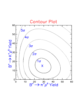
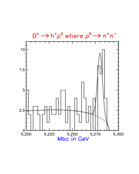
FIG. 4.: Contour and projection plot for $B^{\pm}\rightarrow\pi^{\pm}\rho^{0}$.

TABLE II.: Event Selection for $B\to PV$ decays

Sample	E $-$ Ebeam	Resonance Mass Window	Cos(Resonance Helicity Angle)
$h^{\pm}\rho^{0}$	$|$E($\pi\pi\pi$)$-$Ebeam$|<$100MeV	200MeV	$-$0.9 $-$ 0.9
$h^{\pm}K^{*0}$	$|$E($\pi K\pi$)$-$Ebeam$|<$100MeV	75MeV	$-$0.9 $-$ 0.9
$h^{\pm}\rho^{\mp}$	$|$E($\pi\pi\pi^{0}$)$-$Ebeam$|<$150MeV	200MeV	0.0 $-$ 0.9
$h^{\pm}K^{*\mp}(K^{\mp}\pi^{0})$	$|$E($\pi K\pi^{0}$)$-$Ebeam$|<$300MeV	200MeV	0.1 $-$ 1.0
$h^{\pm}K^{*\mp}(K^{0}_{s}\pi^{\mp})$	$|$E($\pi K\pi^{0}$)$-$Ebeam$|<$200MeV	200MeV	$-$0.86 $-$ 1.0

The contribution of $b\rightarrow c$ and other related rare $B$ processes are small but not negligible. They are evaluated using about 25 million generic b$\bar{\mbox{b}}$ Monte Carlo events, and specific Monte Carlo samples for all the rare $B$ processes mentioned in this paper. The dominant contributions are listed in Table III. All other contributions are negligible.

TABLE III.: Contributions to the $B^{\pm}\rightarrow\pi^{\pm}\rho^{0}$ Yield from Non-continuum physics backgrounds

Decay Process	Contribution to $B^{\pm}\rightarrow\pi^{\pm}\rho^{0}$ Yield
b $\rightarrow$ c	0.9$\pm$0.7
$B^{0}\rightarrow\pi^{+}\rho^{-}$	0.7$\pm$0.3
$B^{0}\rightarrow K^{+}\rho^{-}$	0.1$\pm$0.1
$B^{0}\rightarrow\pi^{+}K^{*0}$	0.3$\pm$0.2
TOTAL	2.0$\pm$0.8

The final $B^{\pm}\rightarrow\pi^{\pm}\rho^{0}$ yield after background subtraction is: 26.1${}^{+9.1}_{-8.0}$ events, leading to a branching fraction measurement of ${\cal B}(B^{+}\to\pi^{+}\rho^{0})=(1.5\pm 0.5\pm 0.4)\times 10^{-5}$. This is the first observed hadronic $b\rightarrow u$ transition.

2 First Observation of $B^{0}\rightarrow\pi^{\pm}\rho^{\mp}$

As discussed above, the $\pi^{0}$ daughter of the $\rho$ has a bi-modal momentum distribution due to the longitudinal polarization (helicity = 0) of the $\rho$. The ratio of real to fake $\pi^{0}$ is roughly $1/2$ for the low and $10/1$ for the high momentum $\pi^{0}$ region. This leads to largely increased backgrounds from all sources as well as multiple entries per event in the low momentum $\pi^{0}$ region. In addition, the charged pion tends to be fast for the slow $\pi^{0}$ region, thus leading to increased $K^{\star+}\leftrightarrow\rho^{+}$ misidentification.

In contrast, the only drawback of the fast $\pi^{0}$ region over the three track sample is a factor two degraded $\Delta E$ resolution. We therefore choose to use only the half of the sample that has a high momentum $\pi^{0}$ in our fits in the two track $\pi^{0}$ final state at this point. Besides this, the same likelihood fits are made as described for the three track final state.

Efficiencies and results are summarized in Table IV. The crossfeed rates from other $PV$ modes as well as $b\to c$ decay backgrounds are negligible. A significant signal in $B^{0}\rightarrow\pi^{\pm}\rho^{\mp}$ is observed at a branching fraction of ${\cal B}(B^{0}\to\pi^{\mp}\rho^{\pm})=(3.5^{+1.1}_{-1.0}\pm 0.5)\times 10^{-5}$. Note that we do not tag the flavor of the $B$ in the present analysis. The measured branching fraction is therefore the sum of $B^{0}\to\rho^{+}\pi^{-}$ and $B^{0}\to\rho^{-}\pi^{+}$. In addition, averaging over charge conjugate states is as always implied.

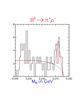
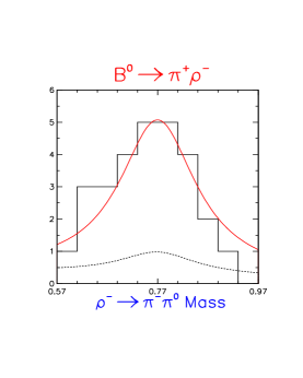
FIG. 5.: Contour and projection plot $B^{0}\rightarrow\pi^{\pm}\rho^{\mp}$.

3 Evidence for $B^{0}\rightarrow\pi^{-}K^{*+}$

We search for $B^{0}\rightarrow\pi^{-}K^{*+}$ with submodes $K^{*+}\rightarrow K^{0}_{S}\pi^{+}$ and $K^{*+}\rightarrow K^{+}\pi^{0}$. Due to the large combinatoric and physics backgrounds in the soft $\pi^{0}$ region, we only select the hard $\pi^{0}$ region for the $K^{+}\pi^{0}$ decay of the $K^{*}$. Backgrounds other than those from continuum are negligible. Event selections are presented in Table II. Efficiencies and results are summarized in Table IV.

The individual branching ratios obtained in the two $K^{*+}$ submodes are consistent, and we combine the two submodes to arrive at an average branching ratio of ${\cal B}(B^{0}\rightarrow\pi^{-}K^{*+})$ = (2.2 ${}^{+0.8\ +0.4}_{-0.6\ -0.5}$) $\times$ 10^-5 which is 5.9$\sigma$ from zero. We note that the statistical significance depends largely on the two track $K^{0}_{s}$ final state, which has less background and larger efficiency than the two track $\pi^{0}$ final state. In contrast to the two observed $B\to\rho\pi$ decays, the one dimensional projections of the fit (see Fig. 6) are somewhat less than inspiring, and a simple event count in the mass plot does result in an excess of only $2.4\sigma$. However, goodness of fit ($21\%CL$), and likelihood per event distributions are perfectly consistent with expectations from Monte Carlo. The most likely signal events have signal likelihoods consistent with what one may expect from signal Monte Carlo, rather than the background data taken below $B\bar{B}$ threshold.

In addition, we generated 25000 distinct Monte Carlo background samples in the $K^{0}_{s}\pi^{+}\pi^{-}$ final state. Each of these samples has the same number of events as our actual data in this final state. We perform a likelihood fit to each of these 25000 samples and record signal yield and significance as reported by each fit. We find that none of these background samples leads to a reported yield or significance as large as found in data. We therefore conclude that our result is exceedingly unlikely to be due to a background fluctuation.

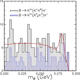
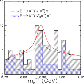
FIG. 6.: Contour and projection plot $B^{0}\rightarrow\pi^{\pm}K^{*\mp}$.

TABLE IV.: Summary of CLEO results for $B$ decays to a pseudo-scalar and a vector mesons ($PV$ modes)

Mode	Eff (%)	Yield	Signif	BR/UL ($10^{-5}$)
$\pi^{\pm}\rho^{0}$	$30\pm 3$	$26.1^{+9.1}_{-8.0}$	5.2$\sigma$	$1.5\pm 0.5\pm 0.4$
$\pi^{\pm}\rho^{\mp}$	$12\pm 1$	$28.5^{+8.9}_{-7.9}$	5.6$\sigma$	$3.5^{+1.1}_{-1.0}\pm 0.5$
$\pi^{\pm}K^{*\mp}(K^{0}_{S}\pi^{\mp})$	$7\pm 1$	$10.8^{+4.3}_{-3.5}$	5.2$\sigma$	$2.3^{+0.9}_{-0.7}\pm 0.3$
$\pi^{\pm}K^{*\mp}(K^{\mp}\pi^{0})$	$4.1\pm 0.4$	$5.7^{+4.3}_{-3.2}$	2.5$\sigma$	$2.0^{+1.5\ +0.3}_{-1.1\ -0.4}$
$\pi^{\pm}K^{*\mp}$			5.9$\sigma$	$2.2^{+0.8\ +0.4}_{-0.6\ -0.5}$
$\pi^{\pm}K^{\star 0}(K^{+}\pi^{-})$	$18\pm 2$	$12.3^{+5.7}_{-4.7}$	$<$ 3$\sigma$	$<$ 2.7
$K^{\pm}\rho^{0}$	$28\pm 2$	$14.8^{+8.8}_{-7.7}$	$<$ 3$\sigma$	$<$ 2.2
$K^{0}\rho^{0}$	$10\pm 1$	$8.2^{+4.9}_{-3.9}$	$<$ 3$\sigma$	$<$ 2.7
$K^{\pm}\rho^{\mp}$	$11\pm 1$	$8.3^{+6.3}_{-5.0}$	$<$ 3$\sigma$	$<$ 2.5
$K^{\pm}\phi$	$26\pm 3$			$<$ 0.59
$K^{0}\phi$	$7\pm 1$			$<$ 2.8
$\pi^{\pm}\phi$	$26\pm 3$			$<$ 0.40
$\pi^{0}\phi$	$17\pm 2$			$<$ 0.54
$K^{\pm}K^{*\mp}(K^{0}_{S}\pi^{\mp})$	$7\pm 1$	$0.0^{+0.9}_{-0.0}$		$<$ 0.8
$K^{\pm}K^{*\mp}(K^{\mp}\pi^{0})$	$4.1\pm 0.4$	$0.0^{+1.3}_{-0.0}$		$<$ 1.7
$K^{\pm}K^{*\mp}$				$<$ 0.6
$K^{+}K^{*0}(K^{+}\pi^{-})$	$18\pm 2$	$0.0^{+2.1}_{-0.0}$		$<$ 1.2

IV Discussion of our Results

Let us start by summarizing some of the more striking features seen in the data. First of all, we see no evidence for $B\to K\bar{K}$ decays in either $B\to PP$ or $B\to PV$. Such decays would proceed either via highly suppressed $W-$exchange (e.g. $B\to K^{+}K^{-}$) and $b\to d$ penguin diagrams (e.g. $B\to K^{0}_{s}K^{\pm}$, $B\to K^{0}_{s}K^{0}_{s}$) or via final state rescattering (FSI). Given that our upper limits for some of these decays are an order of magnitude smaller than at least some of the branching fractions we measure it seems fair to neglect FSI when trying to understand the dominant contributions to charmless hadronic $B$ decays.

Second, we see no evidence for $B\to\pi\pi$ decays while we observe both $B\to K\pi$ as well as $B\to\rho\pi$ decays. We try to make sense out of this in Section IV A in the context of isospin and factorization.

Third, we are so far unable to measure the branching fraction for any of the $B\to\rho K$ decay modes, despite the fact that we have measured $B\to\rho\pi$ and $B\to K\pi$, and at least one of the $B\to K^{\star}\pi$ decay modes. This is in full agreement with factorization predictions. Factorization predicts destructive (constructive) interference between penguin operators of opposite chirality for $B\to\rho K$ ($B\to K\pi$), leading to a rather small (large) penguin contribution in these decays. In addition, factorization and CVC predict that only the left-handed penguin operator contributes in $B\to K^{\star+}\pi^{-}$. Destructive interference of penguin operators is therefore not expected in this decay mode.

Fourth, we want to note that the measured ratio $R_{\rho}={\cal B}(B^{0}\to\rho^{\pm}\pi^{\mp})/{\cal B}(B^{+}\to\rho^{0}\pi^{+})$ is much smaller than naively expected. In $B\to\rho\pi$ decays the $\rho$ can either come from the upper or lower vertex, and it is generally believed that upper vertex $\rho$ production clearly dominates due to favorable form factors as well as decay constants. In addition, $B^{+}\to\rho^{0}\pi^{+}$ is further suppressed by a factor two because only the $u\bar{u}$ part of the $\rho^{0}$ wave function contributes. The present CLEO measurement of ${\cal B}(B^{0}\to\rho^{\pm}\pi^{\mp})$ is the sum of upper and lower vertex $\rho$ production. It is therefore rather surprising that the measured $R_{\rho}=2.3\pm 1.3$ is not significantly larger than two. Measurements of $B\to\rho^{+}\pi^{0}$ as well as a flavor tagged measurement of $B\to\rho^{+}\pi^{-}$ would help to clarify the situation in $B\to\rho\pi$ decays. It remains to be seen whether or not such measurements are within reach using the full CLEO data set.

Finally, maybe the most striking observation in our data are the large branching fractions measured for charged as well as neutral $B$ decays to $\eta^{\prime}K$. Violation of a sum-rule proposed by Lipkin [19] seems to indicate that a significant flavor singlet contribution is needed to explain these rates. The literature is full [20] of attempts to explain this apparent discrepancy, the most interesting of which is the suggestion that R-parity violating couplings may explain the large $\eta^{\prime}K$ as well as the stringent limit on $\phi K$ [21]. The latter is particularly amusing as one of the relevant couplings ($\lambda^{\prime}_{323}$) would also be present in $B_{s}-$mixing [22] and could therefore lead to a different value for $\gamma$ as inferred from $B\to K\pi$ decays and the limit on $\Delta m_{s}/\Delta m_{d}$ in the context of the usual analysis of the $\rho-\eta$ plane  [30].

A Understanding the non-observation of $B\to\pi\pi$

Most theoretical predictions lead us to expect a branching fraction for $B\to\pi^{+}\pi^{-}$ at a level of $1-2\times 10^{-5}$. [23] Instead, the central value and 90$\%$ confidence level upper limit presented here are $4$ and $8\times 10^{-6}$. With results like this a natural question to ask is “How small can ${\cal B}(B\to\pi^{+}\pi^{-})$ be?”.

Let us start our answer by describing a data based factorization prediction. Assuming factorization, and neglecting W-exchange, penguin annihilation, and electroweak penguin diagrams one may expect the following expressions for the decay amplitudes: [24]

$$\begin{array}[]{ccccc}\sqrt{2}A^{\pm 0}&=&-(T+C)\\ A^{+-}&=&-(T+P)&=&-|T|e^{i\gamma}\times(1-|P/T|e^{i\alpha})\\ \sqrt{2}A^{00}&=&P-C\\ \end{array}$$ (2)

Superscripts $+,-,0$ indicate the charge of the final state pions, and $T,C,P$ stand for external and internal W-emission, and gluonic penguin diagrams respectively (Fig. 1(a), Fig. 1(c), and Fig. 1(b)).

We can arrive at “data based factorization estimates” of these amplitudes if we identify $C=a_{2}/a_{1}\times T$ and use $a_{2}/a_{1}=0.21\pm 0.14$ from measurements in $B\to D$ decays [25]. We then estimate $T$ using factorization and the CLEO measurement ${\cal B}(B\to\pi l\nu)=(1.8\pm 0.5)\times 10^{-4}$ [26] as follows:

$$\begin{array}[]{ccccccccc}T&\sim&\sqrt{6}\pi f_{\pi}&\times&a_{1}&\times&\sqrt{d\Gamma(B\to\pi l\nu)/dq^{2}|_{q^{2}=m_{\pi}^{2}}\over\Gamma(B\to\pi l\nu)}&\times&\sqrt{{\cal B}(B\to\pi l\nu)}\\ &\sim&1.0\mathrm{GeV}&\times&(1.0\pm 0.1)&\times&(0.27\pm 0.05)/\mathrm{GeV}&\times&(0.0135\pm 0.0022)\\ &\sim&\lx@intercol(3.6\pm 0.9)\times 10^{-3}\hfil\lx@intercol\\ \end{array}$$ (3)

The dominant error here is due to the spread among a variety of theoretical models for the $q^{2}$ dependence of the form factor [27]. We do not assign any error due to a possible breakdown of the factorization hypothesis. Throughout this paper we express the absolute size of amplitudes in units of $\sqrt{\mathrm{Branching\ Fraction}}$.

The decay $B^{+}\to K^{0}_{s}\pi^{+}$ has three down type quarks in the final state. Inspection of Figure 1 shows that this final state can only be reached via penguin diagrams, or final state rescattering. Furthermore, the electroweak penguin contribution to this decay is color suppressed, rather than the color allowed one shown in Figure 1(d). It is therefore reasonable to estimate $P$ from the measured ${\cal B}(B\to K^{0}\pi^{\pm})$ corrected by CKM and SU(3) breaking factors.

Using these numbers we arrive at $|T/P|_{d}=5.0\pm 2.3$. This leads to the factorization predictions ${\cal B}(B^{0}\to\pi^{+}\pi^{-})=(8\pm 5)\times 10^{-6}$, ${\cal B}(B^{+}\to\pi^{+}\pi^{0})=(10\pm 5)\times 10^{-6}$, and ${\cal B}(B^{0}\to\pi^{0}\pi^{0})\sim$ few $\times 10^{-6}$. The last of these three estimates is not very meaningful given the errors on the quantities that enter. We assume maximum destructive interference ($\cos\alpha=1$). Ignoring the penguin contribution (i.e. $\cos\alpha=0$) leads to a prediction of ${\cal B}(B^{0}\to\pi^{+}\pi^{-})=(13.0\pm 6.5)\times 10^{-6}$.

As an aside, we can calculate $|T/P|_{s}=0.26\pm 0.08$. This means that CP violating rate asymmetries as large as $50\%$ are in principle possible for decays like $B\to K^{+}\pi^{-}$ if the relevant weak and strong phases are close to $\pm\pi/2$.

In addition to these factorization estimates, it is quite illustrative to look at the isospin decomposition of $B\to\pi\pi$: [2]

$$\begin{array}[]{ccc}\sqrt{2}A^{\pm 0}&=&3A_{3/2}^{\gamma}\times e^{i\delta}\\ A^{+-}&=&{A_{3/2}^{\gamma}\times e^{i\delta}+A_{1/2}^{\gamma}}+{A_{1/2}^{\beta}}\\ \sqrt{2}A^{00}&=&{2A_{3/2}^{\gamma}\times e^{i\delta}-A_{1/2}^{\gamma}}-{A_{1/2}^{\beta}}\\ \end{array}$$ (4)

Here the subscripts $1/2,3/2$ indicate the two different isospin amplitudes. Note that only the $A_{1/2}$ amplitude has any contribution from $b\to d$ penguins, whereas the $A_{3/2}$ amplitude is a pure $b\to u$ transition. We indicate this by making the dependence on weak ($\beta,\ \gamma$) and strong interaction phases ($\delta$) explicit. Using the factorization estimates above, it is easy to show that $|A_{1/2}^{\gamma}|,\ |A_{3/2}^{\gamma}|$, and $|A_{1/2}^{\beta}|$ are of the same order of magnitude.

Equation 4 shows that ${\cal B}(B\to\pi^{\pm}\pi^{0})$ can be estimated without making any assumptions about strong or weak phases. However very little can be said about the relative size of $B\to\pi^{0}\pi^{0}$ versus $B\to\pi^{+}\pi^{-}$ without making such assumptions about relative phases. Common prejudice assumes $\delta<<1$ and therefore $B\to\pi^{+}\pi^{-}\ >>\ B\to\pi^{0}\pi^{0}$ due to the destructive interference between $A_{3/2}$ and $A_{1/2}$ in $B\to\pi^{0}\pi^{0}$. However, as we allow for $\delta$ to increase towards $\pi$ we not only decrease (increase) $B\to\pi^{+}\pi^{-}(\pi^{0}\pi^{0})$ but also increase the size of the “penguin pollution” in any future attempt of measuring $\sin 2\alpha$ via time dependent CP violation in $B\to\pi^{+}\pi^{-}$.

We are thus in the amusing situation that we would like $B\to\pi^{0}\pi^{0}$ to be large to make the Gronau, London isospin decomposition [2] experimentally feasible. Though at the same time, we can only hope for $\delta<<1$ (i.e. vanishingly small $B\to\pi^{0}\pi^{0}$) to avoid destructive interference between the two $b\to u$ pieces in the amplitude for $B\to\pi^{+}\pi^{-}$.

We conclude that our present data is still consistent with factorization predictions for $B\to\pi^{+}\pi^{-}$. However, $B\to\pi^{+}\pi^{-}$ could be significantly smaller than predicted by factorization if the strong interaction phase between isospin amplitudes is non-zero.

B Comment on Neubert-Rosner bound on $\gamma$

As previously mentioned, the ratio $R_{\star}={\cal B}(B^{\pm}\to K^{0}\pi^{\pm})/2{\cal B}(B^{\pm}\to K^{\pm}\pi^{0})$  [8], may be used to constrain $\cos\gamma$ if $R_{\star}\neq 1$. Our measurement of this ratio is $R_{\star}=0.47\pm 0.24$. The relevant equation for bounding $\cos\gamma$ out of the paper by Neubert and Rosner [8] is:

$$\cos\gamma=\delta_{EW}-((1-\sqrt{R_{\star}})/\epsilon_{3/2})/\cos\phi+O(\epsilon_{3/2}^{2})$$ (5)

The parameter $\epsilon_{3/2}$ is defined in terms of experimentally measurable quantities below. It is essentially given by the ratio of $b\to u$ tree and $b\to s$ gluonic penguin amplitudes. The $O(\epsilon_{3/2}^{2})$ terms were shown to be small in Ref. [28]. Here, $\delta_{EW}=0.63\pm 0.15$ is the theoretically calculated contribution from electroweak penguin operators [8].

The dominant uncertainty in Equation 5 is the unknown strong phase $\cos\phi$. Taking the extreme values of $0$ and $\pi$ for this phase we thus arrive at an excluded region for $\cos\gamma$ rather than an actual measurement. To be conservative, one may choose values for $\delta_{EW}$ such as to minimize this excluded region:

$$0.48+|1-\sqrt{R_{\star}}|/\epsilon_{3/2}\geq\cos\gamma\geq 0.78-|1-\sqrt{R_{\star}}|/\epsilon_{3/2}$$ (6)

The structure of this is obviously to exclude values for $\cos\gamma$ near $\cos\gamma=\delta_{EW}$ if $X\equiv|1-\sqrt{R_{\star}}|/\epsilon_{3/2}>0.15$. The size of the exclusion region is determined by the central value of $X$ as well as its error. The variable $X$ defined here is given in terms of measurable quantities up to small uncertainties due to non-factorizable SU(3) breaking:

$$\begin{array}[]{ccc}X\equiv|1-\sqrt{R_{\star}}|/\epsilon_{3/2})&=&|1-a/b|\times a/c\\ a&=:&\sqrt{{\cal B}(B\to K^{0}\pi^{+})}\\ &=&(3.74\pm 0.72)\times 10^{-3}\\ b&=:&\sqrt{2\times{\cal B}(B\to K^{+}\pi^{0})}\\ &=&(5.48\pm 0.91)\times 10^{-3}\\ c&=:&|V_{us}/V_{ud}|f_{K}/f_{\pi}\times\sqrt{2\times{\cal B}(B\to\pi^{+}\pi^{0})}\\ &=&(0.95\pm 0.31\ (0.91\pm 0.18))\times 10^{-3}\\ \end{array}$$ (7)

The two different values for $c$ are obtained using either the most likely value for ${\cal B}(B\to\pi^{+}\pi^{0})$ based on the preliminary CLEO results (including statistical and systematic errors added in quadrature), or a weighted average of the latter with theoretical predictions based on factorization [8]. When calculating $X$ from these numbers we additionaly increase $c$ to conservatively account for theoretical uncertainties due to non-factorizable SU(3) breaking ($``f_{K}/f_{\pi}^{\prime\prime}\equiv 1.33$ rather than the experimental value of $1.2$). The resulting values for $X$ are $1.15\pm 0.62$ and $1.20\pm 0.56$ respectively for the two different values for $c$. In the following we will use $X=1.20\pm 0.56$. A number of comments are in order at this point.

First, the central value for $X$ leads to a physical value for $\cos\gamma$ via Equation 5 only if the strong phase $\phi\sim 0$. In that case, the measured $X$ then prefers rather large values of $|\gamma|\sim 120^{\circ}$. Such values of $\gamma$ are generally not the favored ones as they would tend to imply $B_{s}$ mixing to be smaller than the present limits and/or $f_{B_{s}}\sqrt{B_{B_{s}}}/f_{B_{d}}\sqrt{B_{B_{d}}}$ to be at the large end of the generally assumed range. It was pointed out by He, Hou, and Yang [29] that a number of other charmless hadronic $B$ decay results from CLEO also suggest $|\gamma|>90^{\circ}$.

Second, only $10-15\%$ of a Gaussian with mean $0.48+X$ and $\sigma=\sigma_{X}$ ly within the physically allowed region for $\cos\gamma$. Calculating a bound in this case isn’t all that meaningful. Instead one may consider $\cos\phi<0$ to be ruled out at $\sim 90\%$ confidence level. Using the usual procedure of calculating one-sided confidence levels based on the area inside the physical region only, results in the bound $\cos\gamma\leq 0.33\ @\ 90\%$ confidence level.

Third, the experimental errors on $X$ are large, roughly 1/4 of the physically allowed region total. It is fair to say that the only reason why we may deduce a non-zero exclusion region for $\cos\gamma$ from present measurements is because our present central value for $X$ indicates a prefered value for $\cos\gamma$ that is far away from $\cos\gamma=\delta_{EW}$. This is in contrast to some of the recent analyses of the $\rho-\eta$ plane [30] which tend to favor $\cos\gamma\sim\delta_{EW}$.

V Conclusion

In summary, we have measured branching fractions for three of the four exclusive $B\to K\pi$ decays, as well as the two $B\to\eta^{\prime}K$ decays, while only upper limits could be established for all other $B$ decays to two pseudo-scalar mesons. In addition, we have observed two of the four $B\to\rho\pi$ decays, as well as one of the four $B\to K^{\star}\pi$ decays. We do not observe significant yields for $B$ decays to $\rho K$, $K^{\star}K$, $\phi\pi$ or $\phi K$.

The pattern of observed decays is broadly consistent with expectations from factorization. We see significant contributions from both $b\to u$ as well as $b\to s$ transitions.

In addition, the Neubert-Rosner bound derived from present CLEO data on charmless hadronic $B$ decays indicates $\cos\gamma<0.33\ @\ 90\%$ confidence level. This is in slight disagreement with some of the more aggressive analyses of the $\rho-\eta$ plane found in the literature which prefer larger values of $\cos\gamma$.

Many thanks to our colleagues at CLEO for many stimulating discussions as well as the experimental work that made this paper possible. Further thanks go to A. Ali, J.-M. Gérard, M. Gronau, W.-S. Hou, M. Neubert, J. L. Rosner, and H. Yamamoto for discussions on topics related to Section IV. We gratefully acknowledge the effort of the CESR staff in providing us with excellent luminosity and running conditions.

REFERENCES

- [1] M. Kobayashi and K. Maskawa, Prog. Theor. Phys. 49, 652 (1973).
- [2] M. Gronau and D. London, Phys. Rev. Lett. 65, 3381 (1990).
- [3] Y. Grossman, H. R. Quinn, Phys. Rev. D 56, 7259 (1997).
- [4] A. E. Snyder, H. R. Quinn, Phys. Rev. D 48, 2139 (1993).
- [5] I. Bediaga, R.E. Blanco, C. Gobel, and R. Mendez–Galain, hep-ph/9804222.
- [6] M. Gronau, J. L. Rosner, and D. London, Phys. Rev. Lett. 73, 21 (1994); R. Fleischer, Phys. Lett. B 365, 399 (1996).
- [7] R. Fleischer and T. Mannel, Phys. Rev. D 57, 2752 (1998).
- [8] M. Neubert and J. L. Rosner, Phys. Lett. B 441, 403 (1998).
- [9] J.-M. Gérard and J. Weyers, Université Catholique de Louvain preprint UCL-IPT-97-18(1997), hep-ph/9711469 (unpublished); M. Neubert, Phys. Lett. B 424, 152 (1998). A. F. Falk, A. L. Kagan, Y. Nir, and A. A. Petrov , Phys. Rev. D 57, 4290 (1998)
- [10] R. Fleischer, CERN-TH/98-128, hep-ph/9804319 (unpublished); M. Gronau and J. Rosner, EFI-98-23(1998), hep-ph/9806348 (unpublished); A. F. Falk, A. L. Kagan, Y. Nir, and A. A. Petrov , Phys. Rev. D 57, 4290 (1998).
- [11] M. P. Worah hep-ph/9711265; D. Guetta, Phys. Rev. D58 116008 (1998); G. Barenboim et al., Phys. Rev. Lett. 80, 4625 (1998); A. Masiero, L. Silvestrini hep-ph/9711401.
- [12] R. Godang et al. (CLEO Collaboration), Phys. Rev. Lett. 80, 3456 (1998); B. H. Behrens et al. (CLEO Collaboration), Phys. Rev. Lett. 80, 3710 (1998); D. M. Asner et al. (CLEO Collaboration), Phys. Rev. D 53, 1039 (1996).
- [13] Y. Kubota et al. (CLEO Collaboration), Nucl. Instrum. Methods Phys. Res., Sec. A320, 66 (1992); T. Hill, 6th International Workshop on Vertex Detectors, VERTEX 97, Rio de Janeiro, Brazil.
- [14] S. L. Wu, Phys. Rep. C 107, 59 (1984).
- [15] R. Brun et al., GEANT 3.15, CERN DD/EE/84-1.
- [16] P. Gaidarev, Ph.D. Thesis Cornell University, August 1997; F. Würthwein, Ph.D. Thesis Cornell University, January 1995.
- [17] G. Fox and S. Wolfram, Phys. Rev. Lett. 41, 1581 (1978).
-
[18]
CLEO conference reports 98-09 (ICHEP98 860) and 98-20 (ICHEP98 858)
may be found at http://www.lns.cornell.edu/public/CONF/1998/CONF98-09/
and http://www.lns.cornell.edu/public/CONF/1998/CONF98-20/ respectively. - [19] Harry J. Lipkin, Phys. Lett. B 445, 403 (1999)
- [20] The following is a very incomplete list: Mohammad R. Ahmady, Emi Kou, hep-ph/9903335; F. Araki, M. Musakhanov, H. Toki, Phys. Rev. D59:037501,1999; T. Feldmann, P. Kroll, B. Stech, Phys. Rev. D58:114006,1998; D. Choudhury, B. Dutta, A. Kundu, hep-ph/9812209; Alexander L. Kagan, Alexey A. Petrov, hep-ph/9707354; Hai-Yang Cheng, B. Tseng, hep-ph/9707316; Igor Halperin, Ariel Zhitnitsky, hep-ph/9704412; A. Datta, X.-G. He, S. Pakvasa, hep-ph/9707259.
- [21] D. Choudhury, B. Dutta, A. Kundu, hep-ph/9812209
- [22] See for example V. Bednyakov, A. Faessler, S. Kovalenko, p.43 hep-ph/990414 .
- [23] N. G. Deshpande and J. Trampetic, Phys. Rev. D 41, 895 (1990); L.-L. Chau et al., Phys. Rev. D 43, 2176 (1991); A. Deandrea et al., Phys. Lett. B 318, 549 (1993); A. Deandrea et al., Phys. Lett. B 320, 170 (1994); G. Kramer and W. F. Palmer, Phys. Rev. D 52, 6411 (1995); D. Ebert, R. N. Faustov, and V. O. Galkin, Phys. Rev. D 56, 312 (1997); D. Du and L. Guo, Zeit. Phys. C 75, 9 (1997); N.G. Deshpande, B. Dutta, and S. Oh, hep-ph/9712445; H. Cheng and B. Tseng, Phys. Rev. D 58 (1998) 094005 ; A. Ali, G. Kramer, and C. Lü, Phys. Rev. D 58, (1998) 094009.
- [24] D. Zeppenfeld, Z. Phys. C, 77 (1981); M. Savage and M. Wise, Phys. Rev. D 39, 3346 (1989), ibid D 40, Erratum, 3127 (1989).
- [25] J. Rodriguez, in Proceedings of the Conference on Physics and Violation, Honolulu, 1997.
- [26] J. Alexander et al. (CLEO Collaboration), Phys. Rev. Lett. 77, 5000 (1996).
- [27] Lawrence Gibbons (private communications).
- [28] M. Neubert, hep-ph/9812396.
- [29] Xiao-Gang He, Wei-Shu Hou, and Kwei-Chou Yang, hep-ph/9902256.
- [30] A. Ali, and D. London, hep-ph/9903535; F. Parodi, P. Roudeau, and A. Stocchi, hep-ph/9903063.