Inclusive Jet and Dijet Production at the Tevatron

Abstract

High energy jet distributions measured since 1992 at the Fermilab Tevatron proton–antiproton collider are presented and compared to theoretical predictions. The statistical uncertainties on these measurements are significantly reduced relative to previous results. The systematic uncertainties are comparable in size to the uncertainty in the theoretical predictions. Although some discrepancies between theory and measurements are noted, the inclusive jet and dijet cross sections can be described by quantum chromodynamics. Prospects for reducing the uncertainty in the theoretical predictions by incorporating Tevatron measurements into the proton parton distributions are discussed. Dijet distributions, in excellent agreement with quantum chromodynamics, set a 2.5 TeV limit on the mass of quark constituents.

1 INTRODUCTION

In the past seven years, quantum chromodynamics (QCD), the accepted theory of quark and gluon interactions, has been confronted with a set of precise and varied measurements of jet production from the Fermi National Accelerator Laboratory proton–antiproton collider. In $p\bar{p}$ collisions, jet production can be understood as a point–like collision of a quark or gluon from the proton and a quark or gluon from the antiproton. After colliding, these scattered partons manifest themselves as sprays of particles or “jets”. The extremely high energy of these interactions provides an excellent opportunity to test our understanding of perturbative QCD (pQCD). In particular, differences between QCD calculations and measured jet processes reveal information about both the partonic content of the proton and the nature of the strong interaction. Further, unexpected deviations may signal the existence of new particles or interactions down to distance scales of $10^{-19}$ meters or less.

Historically, jet measurements have involved tests of QCD at the highest energies and searches for new physics. Prior to 1992, the inclusive jet cross section, one of the most important hadron collider results, had been measured at the ISR $pp$ collider at a center–of–mass energy of $\mbox{$\sqrt{\rm s}$}=63$ GeV [1], the CERN $p\bar{p}$ collider at 546 and 630 GeV [2, 3], and the Fermilab Tevatron $p\bar{p}$ collider at 1800 GeV  [4, 5]. These data span a factor of twenty in beam energy and a factor of two hundred in jet energy transverse to the proton beam ($E_{T}$) and, in general, are reasonably well described by QCD.

Studies of the correlations between the leading two jets of an interaction also test QCD and provide opportunities to search for new physics. Measurements of dijet distributions prior to 1992, such as the invariant mass of the leading two jets or the angular separation between the jets, are also in good agreement with QCD [6, 7, 8, 9, 10]. Using the model of Eichten, Lane, and Peskin  [11] these data are used to search for composite quarks  [2, 3, 4, 5, 8, 9, 10], with the best limits coming from an inclusive jet cross section measurement [5]. In this model excess jet production at large $E_{T}$ relative to QCD is interpreted as the product of quark constituent scattering. Because these data sets are relatively small all searches are limited by statistical precision rather than systematic uncertainties at the highest $E_{T}$. A summary of these inclusive jet and dijet results can be found in the review of QCD by Huth and Mangano  [12].

In 1992, with the advent of high luminosity data collection at the Tevatron, a new era of precise $p\bar{p}$ jet physics began. From 1992–1993 (Run 1A) each of the two collider experiments accumulated $\approx$ 20 $pb^{-1}$ of data and from 1994–1996 (Run 1B) each accumulated $\approx$ 100 $pb^{-1}$. Both data sets were taken at $\mbox{$\sqrt{\rm s}$}=$ 1800 GeV. At the end of Run 1B a small portion of data ( $\approx$ 600 $nb^{-1}$) was taken at $\mbox{$\sqrt{\rm s}$}=$ 630 GeV. The two runs together represent a data set $\approx$ 50 times larger than any preceding data set.

In contrast to previous tests of QCD, the Run 1 jet measurements have statistical uncertainties significantly smaller than experimental or theoretical systematic uncertainties. In fact, the inclusive jet analysis from the Run 1A sample yielded a significant discrepancy between data and contemporaneous theoretical predictions as well as good agreement with previous measurements [13]. In addition to stimulating great excitement over the possibility of departures from QCD, the result motivated a re–evaluation of the uncertainties associated with inclusive jet cross section calculations [14, 15, 16]. Later measurements of the inclusive jet cross section using the Run 1B samples stimulated further discussions since one confirmed [17] the Run 1A measurement while the other was well described by QCD. In addition, subsequent studies have indicated that QCD can describe the observed Run 1A cross section through adjustments to the parton distribution functions (PDFs), which represent the fraction of proton momentum carried by the constituent quarks and gluons.

Independent of the actual high $E_{T}$ behavior of the inclusive jet cross section, the Run 1A and 1B results have revealed large uncertainties in the theoretical predictions. In particular, the PDFs are derived from fits to data from many different experiments, all of which are collected at low energy and extrapolated to Tevatron jet energies. Representation of the uncertainties in the resulting PDFs is a complex issue and has never been precisely resolved. Consequently, the Tevatron collaborations have taken an interest in derivation of the PDFs from information collected at the Tevatron. Measurements of dijet mass distributions and dijet cross sections at a variety of scattering angles provide information on the momentum distributions of the partons. By comparing the different measurements, constraints on the PDFs can be established, and sensitivity to the presence of new physics should ultimately be improved.

This review opens with a description of the theoretical framework behind perturbative QCD and a discussion of the uncertainties associated with predictions. Descriptions of the two detectors in which these measurements were performed and jet reconstruction algorithms are also provided. The review then devotes a section each to the Run 1 measurements of the inclusive jet cross section, the ratio of inclusive cross sections at different beam energies, dijet differential cross sections, and dijet mass and angular distributions. As will be seen, these measurements offer a detailed look into the composition of the proton and the nature of the strong interaction. A conclusion summarizes the results and suggests future avenues of research.

2 PERTURBATIVE QUANTUM CHROMODYNAMICS

2.1 Leading Order and Next–to–Leading Order QCD

The proton–antiproton interaction, a fairly general scattering process, nicely introduces the concepts of leading order and next–to–leading order pQCD. As illustrated in Fig. 1, inelastic scattering between a proton and an antiproton can be described as an elastic collision between a single proton constituent and single antiproton constituent. These constituents are collectively referred to as partons and in QCD are quarks and gluons. The non–colliding constituents of the incoming proton and anti–proton are called beam fragments or spectators. Predictions for jet production are given by folding experimentally determined parton distribution functions $f$ with perturbatively calculated two–body scattering cross sections $\hat{\sigma}$ . See, for example, reference [19] for a detailed discussion. The two ingredients can be formally combined to calculate any cross section of interest:

$\sigma=\sum_{i,j}\int dx_{1}dx_{2}f_{i}(x_{1},\mu^{2}_{F})f_{j}(x_{2},\mu^{2}_{F})\hat{\sigma}[x_{1}P,x_{2}P,\alpha_{s}(\mu^{2}_{R}),Q^{2}/\mu^{2}_{F},Q^{2}/\mu^{2}_{R}]$.

The parton distribution functions $f_{k}(x,\mu^{2}_{F})$ describe the momentum fraction $x$ of the incident hadron momentum $P$ carried by a parton of type $k$ (gluons or quarks). The PDF is defined in terms of the factorization scale $\mu_{F}$. The hard two–body cross section is a function of the momentum carried by each of the incident partons $xP$, the strong coupling parameter $\alpha_{s}$, the scale $Q$ characterizing the energy of the hard interaction, and the renormalization scale $\mu_{R}$. Final state partons manifest themselves as collimated streams or “jets” of particles. This formal description includes no explicit hadronization or fragmentation functions to describe the transition from partons to jets. For most high $E_{T}$ measurements these effects are small and jets are identified as partons.

The two–body scattering has been illustrated in Fig. 1 with a leading order (LO) graph. The cross section for this process is proportional to two powers of the strong coupling parameter, $\alpha_{s}$, which come from the two vertices. Although useful, the LO picture is too simple and has large normalization uncertainties. Next–to–leading order (NLO) or O$(\alpha^{3}_{s})$ calculations include one additional parton emission. A schematic example is shown in the second illustration of Fig. 1. Here a final state quark has radiated an additional gluon and the entire scattering process is proportional to $\alpha^{3}_{s}$. Depending on the proximity of the other partons, a “jet” could result from one or two (combined) partons. This in turn results in parton level predictions for the shape of jets, and for the effects of clustering parameters.

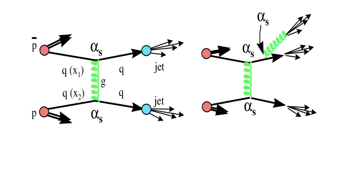
Figure 1: Factorization of the scattering process: In this example incoming quarks with momentum fraction $x_{1}$ and $x_{2}$ of the incident hadrons scatter through gluon exchange and fragment into final state jets.

A complete theoretical prediction of jet production should not depend on internal calculational details; however, this is not the case for fixed order perturbative QCD, which depends on the choice of factorization and renormalization scales. The factorization scale, a free parameter, determines how the contributions of initial state radiation are factorized between the PDFs and $\hat{\sigma}$. The renormalization scale is also arbitrary and is related to choices in the theoretical calculations designed to control or renormalize ultraviolet singularities. Typically, as in this report, $\mu_{R}$ and $\mu_{F}$ are set equal to each other, $\mu_{R}=\mu_{F}=\mu$, and $\mu$ is chosen to be of the same order as $Q$. The sensitivity of the theoretical predictions to $\mu$ is often taken as a measure of the uncertainty from the contributions of higher order terms.

Predictions for jet production at NLO have been derived by Ellis, Kunszt, and Soper [20]; Aversa et al. [21]; and Giele, Glover, and Kosower [22]. The NLO predictions are much less sensitive to the choice of $\mu$ [20]. The “EKS” program by Ellis, Kunszt, and Soper [23] can generate analytic predictions for jet cross sections as a function of final state parameters. The “JETRAD” program by Giele, Glover, and Kosower [24] generates weighted “events” with final state partons. Cross sections are calculated by generating a large number of events as a function of final state parameters. All predictions in this document have been generated either with EKS or JETRAD. The two programs agree within a few percent[16].

2.2 Theoretical Choices

A NLO QCD calculation requires selection of several input parameters including specification of a parton clustering algorithm, a perturbative scale, and PDFs. Taken together these choices can result in approximately 30% variations in the theoretical predictions. The single largest uncertainty is due to the PDFs. These input choices and the resultant changes in the predictions are discussed in the following paragraphs. The variations are illustrated by comparing predictions for the inclusive jet cross section. As in the experimental results to follow, the cross section is reported as a function of jet $E_{T}$ and pseudorapidity $\eta=-{\rm ln}({\rm tan}(\theta/2))$ where $\theta$ is the angle between the jet and the proton beam, and is summed over $\phi$, the azimuthal angle around the beam. For reference, $\eta=0$ for jet production at 90 degrees relative to the proton beam.

2.2.1 PARTON CLUSTERING

The NLO predictions may include two or three final state partons. To convert the partons to the equivalent of jets measured in a detector, a clustering algorithm is employed. The Snowmass cone algorithm [25] was proposed as a way to minimize the difference between theoretical predictions and experimental measurements. In theory calculations, two partons which fall within a cone of radius R in $\eta$–$\phi$ space (R = $\sqrt{\Delta\eta^{2}+\Delta\phi^{2}}$ and $\Delta\eta$ and $\Delta\phi$ are the separation of the partons in pseudorapidity and azimuthal angle) are combined into a “jet”. A standard cone radius of $R=$ 0.7 is used by both collider experiments for most measurements. A consequence of this algorithm is that partons have to be at least a distance of 2R apart to be considered as separate jets.

Subsequent studies indicated that the experimental clustering algorithms (described in later sections) were more efficient at separating nearby jets [26, 27] than the idealized Snowmass algorithm. In other words, two jets would be identified even though they were separated by less than 2R. An additional parameter, $R_{sep}$, was introduced in the QCD predictions to mimic the experimental effects of cluster merging and separation. Partons within $R_{sep}\times R$ were merged into a jet, while partons separated by more than $R_{sep}\times R$ were identified as two individual jets. As described in detail in the references, a value of $R_{sep}$ = 1.3 was found to give the best agreement with the data for cross section and jet shape measurements [26]. This corresponds in the data to the 50% efficiency point in jet separation [27], i.e. two jets within $R_{sep}$=1.3 of one another are merged 50% of the time and identified as two individual jets 50% of the time. At separations of 1.0R the algorithms nearly always merge the two jets and at values of 1.6R they nearly always identify two separate jets. The top panel of Figure 2 shows the change in the prediction for the inclusive jet cross section using the EKS program when $R_{sep}$ is decreased from 2 to 1.3. The result is primarily a normalization change of 5 to 7%.

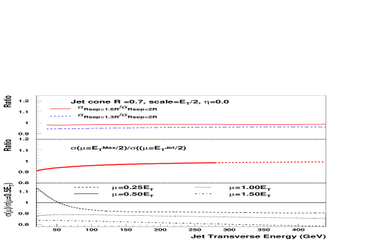
Figure 2: NLO theoretical predictions for the inclusive jet cross section. Each prediction is normalized relative to the NLO EKS calculation with CTEQ4M, $\mu=\mbox{$E_{T}$}^{jet}/2$, $R_{sep}=1.3$.

2.2.2 THE SCALE

Because a NLO calculation is truncated at order $\alpha_{s}^{3}$ there is some residual dependence on the scale $\mu$ at which the calculation is performed. The scale is usually taken to be proportional to $\mbox{$E_{T}$}^{jet}$ (or just $E_{T}$), maximum transverse jet energy $\mbox{$E_{T}$}^{max}$ in a given event, or the total center–of–mass energy. Other choices for the scale are possible. To study the scale dependence of the predictions, the magnitude of the scale is varied by a multiplicative coefficient, common choices are $\mu=0.5\mbox{$E_{T}$}^{jet}$ and $0.5\mbox{$E_{T}$}^{max}$. The middle panel of Fig. 2 shows a mild $E_{T}$ dependence at the 2–9% level on the definition of the scale. The lowest panel shows that typical variations of the multiplicative coefficient lead to 5–20% shifts in the cross section with only small changes in shape above 100 GeV.

2.2.3 PARTON DISTRIBUTION FUNCTIONS

Parton distribution functions are derived from global fits to data primarily from deep inelastic scattering (DIS) fixed target and electron–proton collider experiments. In DIS, a lepton probe is used to sample the partonic structure of the target hadrons. For use at the Tevatron, the resulting distributions must be evolved from the low energy DIS results to the high energy range of jet measurements.

As the data from DIS experiments increases and improves, new parton distribution functions are derived. Some recent PDFs also incorporate data from the Tevatron. The result is a plethora of PDFs, each with its own specific list of data included in the fit, assumptions as to the value of $\alpha_{s}$, functional forms for the quark and gluon momentum distributions, and assumptions concerning the contributions of the gluons, which are not constrained by the DIS results. The most recent PDFs include the most precise data and combined knowledge, and supplant the previous PDFs.

Several groups have analyzed the available data and produced families of candidate PDFs. Within a family, the individual PDFs represent the range of predictions resulting from changes in one of the input assumptions such as the value of $\alpha_{s}$. Additional variations come from differences in the input data sets or the relative weighting between the data sets. The CTEQ2M [28], CTEQ3M [29] and MRSA^′ [30] families of PDFs incorporate data published before 1994 and do not include Tevatron jet data. The CTEQ4M PDFs [31] include data published before 1996; CTEQ4HJ [31] additionally has a high $x$ gluon adjustment designed to accommodate the Run 1A high $E_{T}$ jet cross section measurements. The MRST [32] PDF family utilizes data published before 1998 and adds a contribution for a putative initial transverse momentum of the partons.

Comparison between observed cross sections and NLO predictions with alternate PDFs provide some insight into the quark and gluon composition of the proton. As shown in the Fig. 3 the PDFs can result in $\approx$ 20% variations in jet cross sections; typical variations within a set are on the order of 5–10%. Although the quark distributions were thought to be well known and the contribution of the gluons was expected to be small, investigations [33, 34] have shown that there are uncertainties at high $x$, which were ignored in the derivation of early PDFs. In addition, studies[31] revealed that the gluon distribution could be adjusted to give a significant increase in the jet cross section at high $E_{T}$, while maintaining reasonable agreement with the low energy data sets.

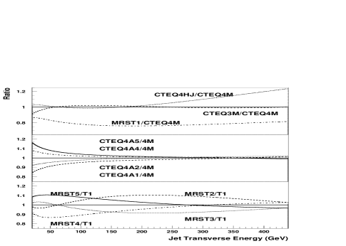
Figure 3: NLO theoretical predictions for the inclusive jet cross section using different PDFs. Each prediction is normalized relative to the NLO EKS calculation with CTEQ4M. All used $\mu=\mbox{$E_{T}$}/2$ and $R_{sep}=1.3$

3 DETECTORS AND JET DEFINITIONS

3.1 The CDF and D0 Detectors

The Collider Detector at Fermilab (CDF) [35] and the D0 Detector [36] at the Fermi National Accelerator Laboratory Tevatron $p\bar{p}$ collider are complementary general purpose detectors designed to study a broad range of particle physics topics. The Tevatron is designed with six locations at which the counter–rotating proton and antiproton beams can collide. The CDF and D0 detectors each occupy one of these interaction regions; D0 takes its name from the alphanumeric designation of its interaction region. Each detector is comprised of a series of concentric sub–systems, which surround the $p\bar{p}$ interaction region. Immediately outside the Tevatron beam pipe each detector has a tracking system designed to detect charged particles. The tracking systems are surrounded by calorimeters, which measure the energy and direction of electrons, photons, and jets. Finally, the calorimeters are covered with muon tracking systems.

Luminosity monitors at each detector measure the beam exposure. These monitors are located near the beam lines and detect particles from the $p\bar{p}$ collisions. The luminosity at a given site is given by dividing the luminosity monitor event rate by that portion of the total $p\bar{p}$ cross section to which the luminosity monitors have acceptance. A direct comparison of jet cross sections at the two experiments is complicated by the fact that the collaborations adopt slightly different values for the total $p\bar{p}$ cross section [37, 38, 39]. As a result, the CDF jet cross section measurements are 2.7% higher than the corresponding D0 jet cross section measurements [37].

In the following sections we mention primarily the central tracking systems and the calorimeters since these systems are the most important for jet identification and reconstruction. As will be seen, CDF has a high resolution particle tracking system, which makes a crucial contribution to jet energy calibration. On the other hand, and in a complementary fashion, D0 has highly segmented, uniform, and thick calorimetry well suited to in–situ jet energy measurements.

Both calorimeters are segmented into projective towers. Each tower points back to the center of the nominal interaction region and is identified by its pseudorapidity and azimuth. The polar angle $\theta$ in spherical coordinates is measured from the proton beam axis, and the azimuthal angle $\phi$ from the plane of the Tevatron. The towers are further segmented longitudinally into individual readout cells. The energy of a calorimeter tower is obtained by summing the energy in all the cells of the same pseudorapidity and azimuth. The transverse energy or $E_{T}$ of a tower is the sum of the $E_{T}$ components of the cells. These components are calculated by assigning each cell of a tower a massless four–vector with magnitude equal to the energy deposited and with the direction defined by the unit vector pointing from the event origin to the center of the tower segment.

3.1.1 D0 in Run 1

The central tracking volume ($\mbox{$|\eta|$}\approx 2$) of D0 includes the vertex chamber, transition radiation detector, and central drift chamber, arranged in three cylinders concentric with the beamline, and two forward drift chambers. The non–magnetic tracker is compact, with an outer radius of 75 cm and an overall length of 270 cm centered on $z=0$. Without the need to measure momenta of charged particles, the prime considerations for tracking were good two track resolving power, high efficiency, and good ionization energy measurement. For jet physics the central tracker is used to find event vertices.

Jet detection in the D0 detector primarily utilizes liquid argon–uranium
calorimeters which are hermetic, finely segmented, thick, uniform and have unit gain. These sampling calorimeters are composed of alternating layers of liquid argon and absorber. The particles in a jet interact with the absorber, and the resulting particle shower ionizes the liquid argon. This ionization is detected as a measure of the jet energy. The calorimeter is enclosed in three cryostats: the central calorimeter (CC) covers $\mbox{$|\eta|$}\leq 1.2$, and the end calorimeters (ECs) extend the coverage to $\mbox{$|\eta|$}\leq 4.4$. The calorimeters have complete $2\pi$ azimuthal coverage. Between the cryostats the calorimeter sampling is augmented by scintillator tiles with segmentation matching the argon calorimeters. Fig. 4 is a graphical representation of the calorimeter modules described below.

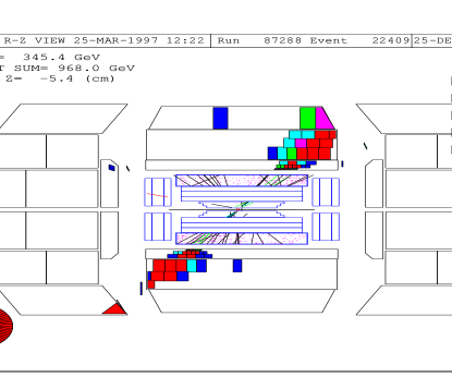
Figure 4: The distribution of energy in a dijet event in the D0 detector.

The CC includes three concentric rings of calorimeter modules. There are 32 electromagnetic calorimeter modules (CCEM) in the inner ring, 16 fine hadronic modules (CCFH) in the middle ring, and 16 coarse hadronic modules (CCCH) in the outer ring. The CCEM and CCFH calorimeters have uranium absorber plates, and the CCCH has copper absorber plates. Longitudinal segmentation includes seven samples: four in the CCEM, three in the CCFH, and one in the CCCH. At $\eta=0$ the CC has a thickness of 7.2 nuclear absorption lengths. The calorimeter cells are segmented into $\Delta\eta\times\Delta\phi=0.1\times 0.1$ except at shower maximum in the third layer of the CCEM where the segmentation is $0.05\times 0.05$. The calorimeter segmentation is designed to form projective towers of size $\Delta\eta\times\Delta\phi=0.1\times 0.1$ geometry which point to $z=0$. In the CC because of the finer resolution in the third layer of the CCEM each tower is comprised of eleven cells.

The two mirror–image ECs contain four module types. An electromagnetic module (ECEM) surrounding the beam pipe is backed by an inner hadronic module (ECIH) which also surrounds the pipe. Outside the ECEM and ECIH are concentric rings of 16 middle and outer hadronic modules (ECMH and ECOH). The ECEM and ECIH have uranium absorber plates and four longitudinal segments. The ECMH has four uranium absorber segments nearest the interaction point and one stainless steel absorber segment behind. The ECOH employs stainless steel plates and includes three longitudinal segments. At $|\eta|$= 2.0 a jet encounters 8–9 longitudinal segments and a nuclear interaction thickness of $\approx 10\lambda_{o}$. The transverse segmentation is similar to that of the CC. The CC(EC) electron energy resolution is $14.8(15.7)\%/\sqrt{E}$ plus 0.3(0.3)% added in quadrature and for hadrons $47.0(44.6)\%/\sqrt{E}$ plus 4.5(3.9)% added in quadrature.

The calorimeter response to the different types of particles is the most important aspect of the D0 jet energy calibration. Electromagnetically interacting particles, like photons ($\gamma$) and electrons deposit most of their energy in the electromagnetic sections of the calorimeters. Hadrons, by contrast, lose energy primarily through nuclear interactions and extend over the full interaction length of the calorimeter. In general, the calorimeter response to the electromagnetic ($e$) and nuclear or hadronic components ($h$) of hadron showers is not the same. Non–compensating calorimeters have a response ratio $e/h$ greater than one and suffer from non-Gaussian event–to–event fluctuations in the fraction of energy lost through electromagnetic production. Such calorimeters give a non-Gaussian signal distribution for hadrons and jets. The D0 calorimeter is nearly compensating and the hadronic and jet response are well described by a Gaussian distribution [40]. In fact, single jet resolution as measured with dijet events has a Gaussian line–shape and is approximately 7% at 100 GeV and 5% at 300 GeV  [41].

The D0 jet calibration requires correction for the hadronic response of the jet; showering of energy outside the cone; and subtraction of an offset which can be attributed to instrumental effects, pile–up from previous beam–beam crossings, additional interactions, and spectator energy. These corrections are derived primarily in–situ [40]. The correction for hadronic response begins with the electromagnetic calibration of the calorimeter which is performed with dielectron and diphoton decays of the $Z$ and $\pi^{0}$ resonances since electrons and photons deposit their energy in the electromagnetic calorimeters. The hadronic response for centrally produced $\gamma$–jet events is derived from data using $E_{T}$ balance between the photon and jet. Because of the rapidly falling $\gamma$–jet cross section the central calorimeter balance technique is limited to jet energies below 150 GeV. Balancing central, well measured photons against high rapidity jets permits the energy calibration to exceed 300 GeV. The response calibration is extended above 300 GeV using simulated $\gamma$–jets events. For a R=0.7, 100 GeV jet at $\eta=0$ the hadronic response is about $0.85\pm 0.01$. The showering correction for this jet is about $1\pm 1$% and is derived from a study of jet profiles. The total offset correction for a R=0.7 jet at $\eta=0$ as determined from a study of data sets with various triggering and luminosity conditions is about $2.6\pm 0.3$ GeV. The contribution from the underlying event or spectator energy alone is roughly $0.9\pm 0.1$ GeV. At $\eta=0$ the mean total energy correction for a R=0.7, 100 GeV jet is $15.0\pm 1.7$% and decreases slowly with energy.

3.1.2 CDF in Run 1

The CDF central ($\mbox{$|\eta|$}\approx 1$) tracking system has three sub–systems located within a 1.5 T magnetic field, that is provided by a superconducting solenoid coaxial with the beam. Nearest the beam, a four–layer silicon microstrip vertex (SVX) detector [42] occupies the radial region between 3.0 and 7.9 cm from the beamline and provides precision $r-\phi$ measurements. Outside the SVX a vertex drift chamber (VTX) provides $r$–$z$ tracking information and is used to locate the position of the $p\bar{p}$ interaction (event vertex) in $z$, along the beam line. Both the SVX and the VTX are mounted inside a 3.2 m long drift chamber called the central tracking chamber (CTC). The radial coverage of the CTC is from 31 to 132 cm. The momentum resolution [35] of the SVX–CTC system is $\delta P_{T}/P_{T}^{2}=[(0.0009P_{T})^{2}+(0.0066)^{2}]^{1/2}$ where $P_{T}$ has units of GeV/c. The CTC provides in–situ measurement of the calibration and response of the calorimeter to low energy particles (where test beam information is not available) along with measurements of jet fragmentation properties.

The solenoid and tracking volumes of CDF are surrounded by calorimeters, which cover $2\pi$ in azimuth and $\mbox{$|\eta|$}\leq 4.2$. The central electromagnetic (CEM) calorimeter covers $\mbox{$|\eta|$}\leq 1.1$ and is followed at larger radius by the central hadronic calorimeters (CHA and WHA) which cover $\mbox{$|\eta|$}\leq 1.3$. These calorimeters use scintillator as the active medium. The CEM absorber is lead and the CHA/WHA absorber is iron. The calorimeters are segmented into units of 15 degrees in azimuth and 0.1 pseudorapidity. Two phototubes bracket each tower in $\phi$ and the average of the energy in the two tubes is used to determine the $\phi$ position of energy deposited in a tower. The interaction length of both the CHA and WHA is $4.5\lambda_{o}$. Electron energy resolution in the CEM is $13.7\%/\sqrt{E}$ plus 2% added in quadrature. For hadrons the single particle resolution depends on angle and varies from roughly $50\%/\sqrt{E}$ plus 3% added in quadrature in the CHA to $75\%/\sqrt{E}$ plus 4% added in quadrature in the WHA. In the forward regions ($1.1<\mbox{$|\eta|$}<4.2$) calorimetric coverage is provided by gas proportional chambers. The plug electromagnetic (PEM) and hadronic calorimeters (PHA) cover the region from $1.1<\mbox{$|\eta|$}<2.4$. The forward electromagnetic (FEM) and hadronic calorimeters (FHA) cover the region from $2.2<\mbox{$|\eta|$}<4.2$. The segmentation of these detectors is roughly 0.1 in $\eta$ and 5 degrees in $\phi$.

Figure 5 shows a 3–jet event in the CDF calorimeter. In this “lego” plot the calorimeter is “rolled out” onto the $\eta$–$\phi$ plane. The tower height is proportional to the $E_{T}$ deposited in the tower. The darker and lighter shading of each tower corresponds to the $E_{T}$ of the electromagnetic and hadronic cells of the tower respectively. The oval around each clump of energy indicates the jet clustering cone described in the next section.

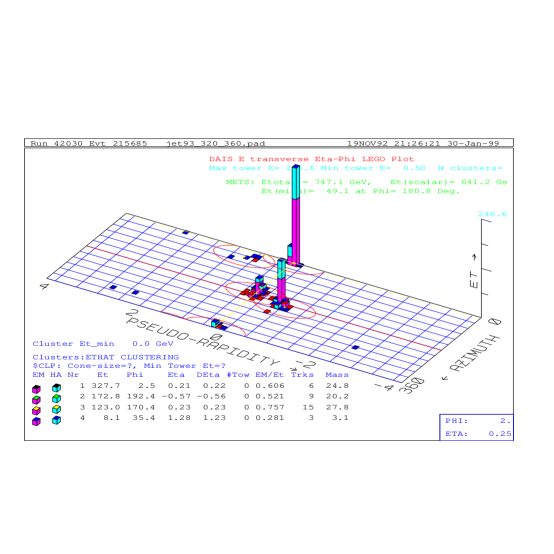
Figure 5: A 3–jet event in the CDF detector. A jet clustering cone of radius 0.7 is shown around each jet.

Observed jet energies are corrected for a number of effects including the calibration and response of the detectors and the background energy from the remnants of the $p\bar{p}$ interaction. In the central detectors corrections associated with detector response are obtained from a Monte Carlo program, which is tuned to give good agreement with the data from electron and hadron test beams ($E_{beam}$ ranged from 10 to 227 GeV), and to data from an in–situ study using CTC track momenta and isolated hadrons with 400 MeV/c$<P_{T}<$ 10 GeV/c. In addition, the Monte Carlo jet fragmentation parameters were tuned to agree with both the number and momenta of particles observed in jets. The resulting simulation was then used to determine “response functions”, which represent the response of the calorimeter to jets as a function of jet $E_{T}$. The width of the response functions represents the jet energy resolution and can be expressed as $\sigma$ = 0.1$E_{T}$ + 1 GeV [5]. Calibration of the plug and forward detectors is achieved through a dijet balancing technique [43]. The $E_{T}$ of jets in the plug and forward detectors is balanced against jets in the central region whose calibration is pinned by the tracking information. The energy left in a jet cone from the hard interaction spectators is called the “underlying event energy”. A precise theoretical definition of this quantity does not exist. Experimentally, it has been estimated from events in which there is no hard scattering, and from the energy in cones perpendicular to the jet axis in dijet events. For a cone of radius 0.7 the contribution to the jet $E_{T}$ is of order 1 GeV. An uncertainty of 30% is assigned to this quantity to cover reasonable variations in the definition of this quantity. The magnitude of the total jet energy corrections and the corresponding uncertainty depend on the $E_{T}$ of the jets and their location in the detector, and on the specific analysis. Typically, the jet $E_{T}$ correction factor is in the range of 1.0 to 1.2.

3.1.3 CDF and D0 in Run 2

The Fermilab Tevatron is undergoing major improvements for Run 2, which is slated to begin in the year 2000. The energy of the proton and antiproton beams will increase from 900 to 1000 GeV and the instantaneous luminosity will increase by at least a factor of 5. The expected Run 2 data sample is 2$fb^{-1}$ in the first 2 years of operation.

Both the CDF and D0 collaborations are improving their detectors for Run 2 operations. Among other things, CDF is replacing the gas calorimeters with scintillating tiles and is closing gaps between calorimeters. CDF is also extending the tracking such that calibration of the new plug detector can be accomplished using tracks, as in the central detector. D0 is also upgrading a number of detector components. For jet measurements the most important upgrade is the replacement of the nonmagnetic tracking system with a magnetic tracker. The tracker (including a high resolution silicon strip detector, a scintillating fiber tracker, and electron/photon preshower detectors) will enable calibration of the calorimeter with single particles. Thus, in Run 2 the detectors will be more similar than in Run 1: CDF will have more uniform calorimetry and D0 will have magnetic tracking. The result of these improvements should be an overall reduction of jet measurement uncertainties.

3.2 The Experimental and Theoretical Definitions of a Jet

From the experimental point of view, jets are the manifestation of partons as showers of electromagnetic and hadronic matter. Jets are observed as clusters of energy located in adjacent detector towers. Typically, a jet contains tens of neutral and charged pions (and to a lesser extent kaons), each of which showers into multiple cells. A single jet illuminates roughly 20 towers (this corresponds to approximately 40 calorimeter cells in the CDF detector and over one hundred detector cells in the D0 detector). Fig. 4 illustrates the energy distribution of a two–jet event in the D0 detector. Each rectangular outline represents the energy deposited in calorimeter cells at fixed $\eta$ and depth. The eye quite naturally clusters the energy into two jet–like objects. However, for the purposes of jet cross section measurements a more quantitative definition of the jet is required.

For high $E_{T}$ measurements at CDF and D0, cone algorithms are used to identify jets in the calorimeters. Cone algorithms operate on objects in pseudorapidity and azimuth space, such as particles, partons, calorimeter cells, or calorimeter towers. For the sake of simplicity towers will be used in the following discussions. The CDF and D0 algorithms are both based on the Snowmass algorithm [25]. This algorithm defines a jet as those towers within a cone of radius $\Delta R=\sqrt{\Delta\phi^{2}+\Delta\eta^{2}}$ = 0.7. The jet $E_{T}$ is the sum of the transverse energies of the towers in the cone, and the location of the jet is defined by the $E_{T}$ weighted $\eta$ and $\phi$ centroids:

$$E_{T}^{jet}=\sum_{i}\mbox{$E_{T}$}^{i}$$

$$\eta_{jet}=(\sum_{i}\mbox{$E_{T}$}^{i}\eta_{i})/\mbox{$E_{T}$}^{jet}$$

$$\phi_{jet}=(\sum_{i}\mbox{$E_{T}$}^{i}\phi_{i})/\mbox{$E_{T}$}^{jet}.$$

The sum over $i$ is over all towers that are within the jet radius $R$.

In Figure 5 the clustering cone is shown by the oval around each jet and is centered on the cluster centroid. The two overlapping cones in this event indicate that the two nearby clusters have been identified as two separate jets. The Snowmass algorithm doesn’t specify cell thresholds or the handling of such overlapping jet cones. These details must be dealt with according to the needs of individual experiments, and led to the introduction of the $R_{sep}$ parameter in the theoretical calculations.

In the D0 experiment, jets are defined in two stages  [27]. In the first or clustering stage, all the energy that belongs to a jet is accumulated, and in the second stage, the $\eta,$ $\phi$ and $E_{T}$ of the jet are defined. The clustering consists of the following steps: 1) Calorimeter towers with $E_{T}$ $\geq$ 1 GeV are enumerated. Starting with the highest $E_{T}$ tower, preclusters are formed by adding neighboring towers within a radius of R=0.3. 2) The jet direction is calculated for each precluster using the sums defined for the Snowmass algorithm. 3) All the energy in the towers in a cone of radius R=0.7 around each precluster is accumulated and used to recalculate $\eta$ and $\phi$. 4) Steps 2 and 3 are repeated until the jet direction is stable. Finally, in the second stage, the jet energy and directions are calculated according to the equations:

$$E^{jet}=\sum_{i}E^{i},~{}~{}~{}\mbox{$E_{T}$}^{jet}=\sum_{i}E_{T}^{i}$$

$$\tan\theta_{jet}=\frac{\sqrt{(\sum_{i}E^{i}_{x})^{2}+(\sum_{i}E^{i}_{y})^{2}}}{\sum_{i}E^{i}_{z}}$$

$$\phi_{jet}=\tan^{-1}[\sum_{i}E^{i}_{y}/\sum_{i}E^{i}_{x}]^{2}$$

where $E^{i}_{x}=E_{i}\sin(\theta_{i})\cos(\phi_{i})$, $E^{i}_{y}=E_{i}\sin(\theta_{i})\sin(\phi_{i})$, and $E^{i}_{z}=E_{i}\cos(\theta_{i})$. Studies have shown that for $\eta\leq\sim 1$ the final D0 jet directions are, within experimental errors, equal to the Snowmass directions. Overlapping jets are merged if more than 50% of the smaller jet $E_{T}$ is contained in the overlap region. If less than 50% of the energy is contained in the overlap region, the jets are split into two jets and the energy in the overlap region is assigned to the nearest jet. After merging or splitting the jet directions are recalculated.

The CDF cluster algorithm [44] has two stages of jet identification similar to the D0 algorithm. The first stage consists of the following steps: 1) a list of towers with $E_{T}>$1.0 GeV is created; 2) preclusters are formed from an unbroken chain of contiguous seed towers with continuously decreasing tower $E_{T}$; if a tower is outside a window of $7\times 7$ towers surrounding the seed it is used to form a new precluster; 3) the preclusters are grown into clusters by finding the $E_{T}$ weighted centroid and collecting the energy from all towers with more than 100 MeV within R=0.7 of the centroid; 4) a new centroid is calculated from the set of towers within the cone and a new cone drawn about this position; steps 3 and 4 are repeated until the set of towers contributing to the jet remains unchanged; 5) overlapping jets are merged if they share $\geq$75% of the smaller jet’s energy; if they share less, the towers in the overlap region are assigned to the nearest jet. In the second stage, the final jet parameters are computed. The angles and energy are calculated as in the D0 algorithm, however the jet $E_{T}$ is given by:

$$\mbox{$E_{T}$}=E\sin\theta_{jet}.$$

One philosophical difference between the CDF and Snowmass algorithms is that the CDF jets have mass ($E_{T}\neq P_{T}$). Studies [25] found that the CDF clustering algorithm and the Snowmass algorithm were numerically very similar.

Both the CDF and D0 algorithms are based on the Snowmass algorithm, but the reality of jets of hadrons measured by a finitely segmented calorimeter necessitates the introduction of additional steps and cuts. Apart from small definitional details, the most significant difference between the Snowmass algorithm and its experimental implementations is the handling of cluster merging and separation. To simulate these effects in the NLO calculations the $R_{sep}$ parameter was introduced. Considering the complexity of the hadronic showers is it remarkable that a NLO calculation, with only 2 or 3 partons in the final state and a single additional parameter can provide a good description of the observed jet shapes and cross sections [26].

4 THE INCLUSIVE JET CROSS SECTION AT 1800 GEV

4.1 Introduction

The inclusive jet cross section represents one of the most basic tests of QCD at a hadron–hadron collider. It reflects the probability of observing a hadronic jet of a given $E_{T}$ and rapidity in a $p\bar{p}$ collision. The term inclusive indicates that all the jets in an event are included in the cross section measurement and that the presence of additional non–jet objects (for example electrons or muons) is irrelevant. Theoretical calculations are normally expressed in terms of the invariant cross section:

$Ed^{3}\sigma/dp^{3}$

where $E$ and $p$ are the jet energy and momentum. In terms of the natural experimental variables, the cross section is given by

$d^{2}\sigma/d\mbox{$E_{T}$}d\eta$

which is related to the first expression by,

$Ed^{3}\sigma/dp^{3}=(1/2\pi E_{T})d^{2}\sigma/d\mbox{$E_{T}$}d\eta.$

Massless jets have been assumed ($P_{T}$ = $E_{T}$); the $2\pi$ comes from the integration over the azimuthal angle $\phi$. The measured cross section is simply the number of jets $N$ observed in an $\eta$ and $E_{T}$ interval normalized by the total luminosity exposure, $\cal{L}$:

$d^{2}\sigma/d\mbox{$E_{T}$}d\eta=N/(\Delta\mbox{$E_{T}$}\Delta\eta\cal{L})$.

The CDF and D0 inclusive jet analyses place similar requirements on the events and jets selected for calculation of the cross sections. Both collaborations eliminate poorly measured events by requiring the event vertices to be near the center of the detector. Backgrounds (such as cosmic rays) are eliminated by rejecting events with large missing $E_{T}$. Spurious jets from cosmic ray or instrumental backgrounds are eliminated with quality cuts based on jet shapes. Corrections are made to the measured cross sections to account for the event and jet detection inefficiencies, mismeasurement of the jet energies, and for energy falling in a jet cone from other sources (such as remnants of the $p\bar{p}$ collision, or additional $p\bar{p}$ interactions). No corrections are made for partons showering outside the jet cone as this should be included in the NLO theoretical calculations.

We begin our discussion of the inclusive jet cross section with measurements by the CDF collaboration. The Run 1A measurement stimulated interest due to a discrepancy with QCD predictions at high $E_{T}$. A subsequent measurement by the D0 collaboration with Run 1B data is well described by theoretical predictions, while the preliminary CDF Run 1B result is in good agreement with the 1A measurement. In the next sections, the CDF and D0 measurements are each described in some detail and then comparisons of the two results are presented.

4.2 The CDF Cross Section

In 1996 CDF published the inclusive jet cross section measured from the Run 1A data sample [13] for jet $E_{T}$ from 15 to 440 GeV in the central rapidity range 0.1$\leq|\eta|\leq$ 0.7. This analysis followed the same procedures as previous measurements [4, 5] for correcting the cross section and for estimating the systematic uncertainties. This process will be described briefly below. More detail is available in references [4, 5, 13, 45].

The measured jet $E_{T}$ spectrum requires corrections for energy mismeasurement and for smearing effects caused by finite $E_{T}$ resolution. This is accomplished with the “unsmearing procedure” described in [45]. As mentioned earlier, a Monte Carlo simulation program [5] tuned to the CDF data is used to determine detector response functions. A trial true (unsmeared) spectrum is smeared using these response functions and compared to the raw data. The parameters of the trial spectrum are iterated to obtain the best match between the smeared trial spectrum and the raw data. The corresponding unsmeared curve is referred to as the “standard curve”, and is used to correct the measured spectrum. The simultaneous correction for response and resolution produces a result which is independent of the $E_{T}$ binning used in the measurement while preserving the statistical uncertainty on the measured cross section. For jet $E_{T}$ between 50 and about 300 GeV these corrections increase both the $E_{T}$ and the cross section by $\approx$10%. At lower and higher $E_{T}$ the cross section corrections are larger due to the steepening of the spectrum.

Figure 6 shows the CDF measurement of the inclusive jet cross section from the 20 $pb^{-1}$ Run 1A data sample compared to a NLO prediction from the EKS program with $\mu=E_{T}/2$, $R_{sep}$ = 2.0 and MRSD0’ PDFs. The inset shows the cross section on a logarithmic scale. There is good agreement between data and theory over eleven orders of magnitude. The main figure shows the percentage difference between the data (points) and theory. The bars on the points represent the statistical uncertainty. While excellent agreement is observed below 200 GeV, an excess of events over these theoretical predictions is observed at high $E_{T}$. Predictions with other PDFs which were available at the time are shown by the additional curves. For these predictions the percentage from the default theory (MRSD0’) is shown. As can be seen from the figure, the best agreement below 200 GeV is with the MRSD0’ PDF. Other PDFs agree less well, and none show the rise at high $E_{T}$ observed in the data.

Figure 6: Inclusive jet cross section measured by CDF using the Run 1A data sample compared to predictions from the EKS program with $\mu=E_{T}^{jet}/2$, $R_{sep}$ = 2.0 and MRSD0’. The error bars represent the statistical uncertainty on the cross section. The shaded band represents the quadrature sum of the correlated systematic uncertainties. Also shown is the percentage difference between the predictions using other PDFs and the prediction with MRSD0’.

The systematic uncertainties on the Run 1A cross section were evaluated using the procedures in reference [45]. In short, new parameter sets are derived for $\pm 1$ standard deviation shifts in the unsmearing function for each source of systematic uncertainty. The parameters for the Run 1A cross section are given in Reference [13]. Figures 7(a–h) show, for the Run 1A data sample, the percentage change from the standard curve as a function of $E_{T}$ for the seven largest systematic uncertainties: (a) charged hadron response at high $P_{T}$; (b) the calorimeter response to low–$P_{T}$ hadrons; (c) $\pm 1\%$ on the jet energy for the stability of the calibration of the calorimeter; (d) jet fragmentation functions used in the simulation; (e) $\pm 30\%$ on the underlying event energy in a jet cone; (f) detector response to electrons and photons and (g) modeling of the detector jet energy resolution. An eighth uncertainty, an overall normalization uncertainty of $\pm$3.8%, was derived from the uncertainty in the luminosity measurement[46] ($\pm$3.5%) and the efficiency of the acceptance cuts ($\pm$1.5%). The eight uncertainties arise from different sources and are not correlated with each other. The 1$\sigma$ shifts are evaluated by changing only one item at a time in the Monte Carlo simulation, such as high $p_{T}$ hadron response. The resulting uncertainty in the unsmeared cross section is thus 100% correlated from bin to bin, but independent of the other seven uncertainties.

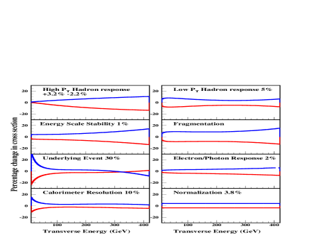
Figure 7: The percentage change in the Run 1A inclusive jet cross section when various sources of systematic uncertainty are changed by $\pm$1 standard deviation from their nominal value.

To analyze the significance of the Run 1A result, the CDF collaboration used four normalization–independent, shape–dependent statistical tests [13]. The eight sources of systematic uncertainty are treated individually to include the $E_{T}$ dependence of each uncertainty. The effect of finite binning and systematic uncertainties are modeled by a Monte Carlo calculation. Between 40 and 160 GeV, the agreement between data and theory is $>$80% for all four tests. Above 160 GeV, however, each of the four methods yields a probability of 1% that the excess is due to a fluctuation. If the test is performed for other PDFs, agreement at low $E_{T}$ is reduced, as is the significance of the excess at high $E_{T}$. The best agreement at high $E_{T}$ for the curves shown is with CTEQ2M[28] which gives 8%, but the low $E_{T}$ agreement is reduced to 23%. The excess of events observed at high $E_{T}$ initiated a re–evaluation of the uncertainties in the PDFs, particularly at high $x$. One outcome of this re–examination was CTEQ4HJ. This PDF incorporates the same low energy DIS data as in CTEQ4M, but the high $E_{T}$ jet data is weighted to accentuate its contribution to the global parton distribution fit in the high $Q$ and $x$ region.

Figure 8 shows the preliminary Run 1B result [47] compared to the Run 1A results and to CTEQ4M (a more modern PDF than the ones in Figure 6). The Run 1A and 1B data sets are in excellent agreement. Only statistical uncertainties are shown. The greatly reduced statistical error bars on the Run 1B data are due to the five–fold increase of luminosity between the two runs. Analysis of the Run 1B data follows exactly the sequence of the Run 1A data with some additional corrections specific to the Run 1B running conditions. The Run 1B systematic uncertainties are very similar to the uncertainties derived for the Run 1A sample. Figure 9 shows the Run 1B result compared to predictions with other recent PDFs. Although CTEQ4HJ is a bit contrived the good agreement with the data demonstrates the flexibility of the PDFs and the ability of the QCD calculations to describe these Run 1A and Run 1B inclusive jet cross sections. Quantitative comparisons between the Run 1B data and theoretical predictions are underway.

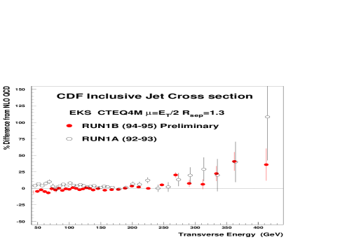
Figure 8: The preliminary Run 1B inclusive jet cross section compared to the published Run 1A data and to a QCD prediction from the EKS program with $\mu$= $E_{T}^{jet}/2$, $R_{sep}$, = 1.3 and CTEQ4M.

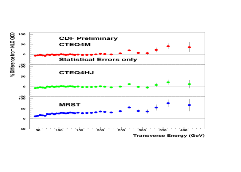
Figure 9: The percent difference between the preliminary Run 1B inclusive jet cross section and QCD predictions from the EKS program with $\mu$= $E_{T}^{jet}/2$, $R_{sep}$ = 1.3, and a variety of current PDFs.

4.3 The D0 Cross Section

In 1998 the D0 collaboration finalized a 92 $pb^{-1}$ measurement of the inclusive jet cross section [18]. The D0 analysis differs from the CDF analysis in that the spectrum is corrected independently for energy calibration and then for distortion by finite jet energy resolution. After passing the various jet and event selection criteria each jet is corrected individually for the average response of the calorimeter. As mentioned in Section 3 the jet response was determined with well measured photon–jet events. However, the background free, energy corrected $E_{T}$ spectrum still remains distorted by jet energy resolution. The distortion is corrected by first assuming that an ansatz function $(A\mbox{$E_{T}$}^{-B})\cdot(1-2\mbox{$E_{T}$}/\sqrt{s})^{C}$ will describe the actual $E_{T}$ spectrum, then smearing it with the measured resolution, and finally comparing the smeared result with the measured cross section. The procedure is repeated by varying parameters $A,B,$ and $C$ until the best fit is found between the observed cross section and the smeared trial spectrum. At all $E_{T}$, the resolution (measured by balancing $E_{T}$ in jet events) is well described by a Gaussian distribution; at 100 GeV the standard deviation is 7 GeV. The ratio of the initial ansatz to the smeared ansatz is used to correct the cross section on a bin–by–bin basis [41]. The resolution correction reduces the observed cross section by (13$\pm$3)% [(8$\pm$2)%] at 60 GeV [400 GeV].

Fig. 10 shows the final inclusive jet cross section as measured by the DO collaboration in the rapidity region $\mbox{$|\eta|$}\leq 0.5$ [18]. This rapidity interval was chosen since the detector is uniformly thick (seven or more interaction lengths with no gaps) and both jet resolution and calibration are precise. The figure shows a theoretical prediction for the cross section from JETRAD . There is good agreement over seven orders of magnitude. For the calculation shown here $\mu=0.5E_{T}^{\rm max}$, the PDF is CTEQ3M, and $\cal{R}_{\rm{sep}}$=$1.3$.

Fig. 11 shows the cross section uncertainties. Each curve represents the average of nearly symmetric upper and lower uncertainties. The energy scale uncertainty which varies from 8% at low $E_{T}$ to 22% at 400 GeV dominates all other sources of uncertainty, except at low $E_{T}$, where the 6.1% luminosity uncertainty is of comparable magnitude. The total systematic error is 10% at 100 GeV and 23% at 400 GeV. Although the individual errors are independent of one another each error is either 100% or nearly 100% correlated point–to–point, and the overall systematic uncertainty is highly correlated. Table 1 shows that the bin–to–bin correlations in the full uncertainty for representative $E_{T}$ bins are greater than 40% and positive. The high degree of correlation will prove a powerful constraint on data–theory comparisons.

Table 1: D0 Inclusive jet cross section total uncertainty correlations.

$E_{T}$ (GeV)	64.6	104.7	204.8	303.9	461.1
64.6	1.00	0.96	0.85	0.71	0.40
104.7	0.96	1.00	0.92	0.79	0.46
204.8	0.85	0.92	1.00	0.91	0.61
303.9	0.71	0.79	0.91	1.00	0.67
461.1	0.40	0.46	0.61	0.67	1.00

Figure 12 shows the ratios $(D-T)/T$ for the D0 data ($D$) and JETRAD NLO theoretical predictions ($T$) based on the CTEQ3M, CTEQ4M and CTEQ4HJ for the region $\mbox{$|\eta|$}\leq 0.5$. Figure 13 shows the same ratios for the $0.1\leq\mbox{$|\eta|$}\leq 0.7$ data. Given the experimental and theoretical uncertainties, the predictions are in agreement with the data; in particular, the data above 350 GeV show no indication of a discrepancy relative to QCD. The D0 collaboration has quantitatively compared the data and theory with a $\chi^{2}$ test incorporating the uncertainty covariance matrix. The matrix elements are constructed by analyzing the mutual correlation of the uncertainties in Fig. 11 at each pair of $E_{T}$ values. Table 2 lists $\chi^{2}$ values for several JETRAD predictions incorporating various PDFs. Each comparison has 24 degrees of freedom. The JETRAD predictions have been fit to a smooth function of $E_{T}$. All five predictions describe the $\mbox{$|\eta|$}\leq 0.5$ cross section very well (the probabilities for $\chi^{2}$ to exceed the listed values are between 47 and 90%). A similar measurement in the $0.1\leq\mbox{$|\eta|$}\leq 0.7$ interval is also well described (probabilities between 24 and 72%). The probabilities calculated by comparing the data to EKS predictions for $\mu=(0.25,0.5,1.0)\times E_{T}^{\rm max}$ and $\mu=(0.25,0.5,1.0)\times E_{T}^{\rm jet}$ are all greater than 57% . Perturbative QCD is in good agreement with the data with or without large $x$ enhancements to the PDFs.

Table 2: $\chi^{2}$ comparisons between JETRAD and DO , $\mbox{$|\eta|$}\leq 0.5$ and $0.1\leq\mbox{$|\eta|$}\leq 0.7$ data for $\mu=0.5E_{T}^{\rm max}$, $\cal{R}_{\rm{sep}}$=$1.3\cal{R}$, and various PDFs. There are 24 degrees of freedom.

PDF	$\mbox{$|\eta|$}\leq 0.5$	$0.1\leq\mbox{$|\eta|$}\leq 0.7$
CTEQ3M	23.9	28.4
CTEQ4M	17.6	23.3
CTEQ4HJ	15.7	20.5
MRSA´	20.0	27.8
MRST	17.0	19.5

Figure 10: The D0 1800 GeV, $\mbox{$|\eta|$}\leq 0.5$ inclusive cross section. Statistical uncertainties are invisible on this scale. The solid curves represent the $\pm 1\sigma$ systematic uncertainty band on the data.

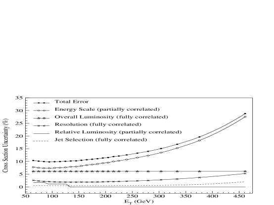
Figure 11: Contributions to the D0 , $\mbox{$|\eta|$}\leq 0.5$ cross section uncertainty plotted by component.

Figure 12: Difference between D0 data and JETRAD QCD predictions with $R_{sep}$ = 1.3 and $\mu=E_{T}^{max}/2$ normalized to predictions for the range $|\eta|<$0.5. The bands represent the total experimental uncertainty.

Figure 13: Difference between D0 data and JETRAD QCD predictions with $R_{sep}$ = 1.3 and $\mu=E_{T}^{max}/2$ normalized to predictions for the range 0.1$<|\eta|<$0.7. The bands represent the total experimental uncertainty.

4.4 Comparison of the CDF and D0 Measurements

The two inclusive jet analyses differ in an important but complementary way. The CDF analysis utilizes a Monte–Carlo program carefully tuned to collider and test beam data, to correct for detector response. In contrast, D0 corrects for calorimeter response by direct utilization of collider data. It is worth mentioning that both collaborations invested years of time and effort developing these procedures. The CDF technique capitalizes on the excellent tracking capabilities of the detector. The tracking is used to directly measure the jet fragmentation functions as well as verify test beam calibrations of the calorimeter modules. Additional checks of the Monte Carlo simulation come from comparisons to collider jet $E_{T}$ balancing data. The uniformity of the D0 calorimetry permits a precise collider data–based measurement of jet response and resolution at all energies and rapidities. This uniformity permits transfer of the jet energy calibration at low to moderate jet energies in the central calorimeter to all pseudorapidity with a missing $E_{T}$ technique. The forward calorimetry provides an opportunity for direct calibration of high energy jets relative to these central photons. The uniformity, linearity and depth of the detector also assures that resolution functions are relatively narrow and Gaussian.

The top half of Fig. 14 shows $(D-T)/T$ for the Run 1B D0 and CDF data sets in the $0.1\leq\mbox{$|\eta|$}\leq 0.7$ region relative to a JETRAD calculation using CTEQ4HJ, $\mu=0.5E_{T}^{\rm max}$, and $\cal{R}_{\rm{sep}}$=$1.3$. Note that there is outstanding agreement between the nominal values for $E_{T}$ $\leq$ 350 GeV. At higher $E_{T}$ the two results diverge but not significantly, given the statistical and systematic errors. This impression is fortified by a direct comparison of the magnitude of the DØ and CDF uncertainties as shown in the second half of the figure. To quantify the degree of agreement, the D0 collaboration has carried out a $\chi^{2}$ comparison between their data and the nominal curve describing the central values of the CDF 1B data. The nominal curve is used instead of the data points because each of the measurements report the cross section at different values of jet $E_{T}$. Comparison of the D0 data to the nominal Run 1B curve, as though it were theory yields a $\chi^{2}$ of 41.5 for 24 degrees of freedom. A ”statistical-error-only” comparison of the D0 and CDF data is approximated by calculating the value of the CDF curve at the D0 $E_{T}$ points and assuming the statistical uncertainty on the CDF and D0 data are equivalent (the D0 statistical errors are multiplied by $\sqrt{2}$.) When the 2.7% relative normalization difference [37] is removed, this statistical-error-only $\chi^{2}$ is 35.1 for 24 degrees of freedom, a probability of 5.4%. When the systematic uncertainties in the covariance matrix are expanded to include both the D0 and CDF uncertainties and the D0 statistical errors are increased by $\sqrt{2}$ the $\chi^{2}$ equals 13.1 corresponding to a probability of $96$%.

Considering the complexities of these analyses, the overall agreement is remarkable! Given the present flexibility of the PDFs and the mixed agreement between the data and theory at the highest $x$ and $Q$, no clear indication of a high $E_{T}$ deviation with QCD can be inferred. By using the high $E_{T}$ jet data, PDFs can be derived which describe both data sets. An unambiguous search for deviations, however, requires an independent measure of the PDFs. Prospects for improvements to the PDFs will be covered in later sections. First we turn our attention to inclusive jet measurements at a different beam energy.

Figure 14: Top: comparisons of D0 and CDF data to JETRAD in the region 0.1$<|\eta|<$0.7. Bottom: the quadrature sums of the DØ and CDF uncertainties.

5 RATIO OF JET CROSS SECTIONS AT TWO BEAM ENERGIES

5.1 Inclusive Jet Cross Sections, Scaling, and the Ratio of Dimensionless Cross Sections

An alternative way to test QCD is to compare the inclusive jet cross sections measured at widely separated center–of–mass energies. The hypothesis of “scaling” predicts that the dimensionless, scaled jet cross section,

$E_{T}^{4}(Ed^{3}\sigma/dp^{3})$,

will be independent of $\sqrt{\rm s}$ as a function of the dimensionless variable $x_{T}=2E_{T}/\sqrt{s}$. This can be written in terms of the experimentally measured quantities as,

$\sigma_{d}=(E_{T}^{3}/2\pi)d^{2}\sigma/d\mbox{$E_{T}$}d\eta$.

QCD predictions depend on the energy scale, or $Q^{2}$, of the interactions and thus suggest that the cross sections should not “scale”. The running of the strong coupling and the evolution of the PDFs are manifestations of this energy (or scale) dependence of the predictions.

Measurement of the ratio of the scaled jet cross sections from two different center–of–mass energies but in the same experimental apparatus, provides a test of QCD in which many theoretical and experimental uncertainties cancel. Figure 15 shows the ratio of the scaled cross sections, $\sigma_{d}^{630}/\sigma_{d}^{1800}$, calculated with JETRAD. The top two panels in the figure show a 10% variation in the ratio below $x_{T}$ = 0.4 (jet $E_{T}$ = 360 GeV at $\sqrt{\rm s}$=1800 GeV) due to the choice of scale. The bottom two panels of Fig. 15 demonstrate that PDF choices produce variations below 10%.

5.2 Jet Production at 630 GeV

In Dec. 1995 CDF and D0 each collected $\approx$600 nb^-1 at $\sqrt{s}$=630 GeV (beam energies of 315 GeV). A primary motivation for this data run was the hope that the inclusive jet cross section at this reduced energy and the ratio relative to 1800 GeV would shed light on the deviations seen with the Run 1A 1800 GeV cross section. The analysis of the 630 GeV data follows an identical path to the analysis described above for the 1800 GeV data. The preliminary measurements from CDF [48] and D0 [49] of the inclusive cross section at $\sqrt{s}=$630 GeV are shown in Fig. 16. The CDF measurement is for the region $0.1\leq\mbox{$|\eta|$}\leq 0.7$ while the D0 result is for the region $\mbox{$|\eta|$}\leq 0.5$. The figure shows the percent difference between the data and the associated theory prediction. The NLO theoretical predictions used the MRSA’  PDF and $\mu=0.5E_{T}^{jet}$. The two measurements are in agreement above 80 GeV, but some discrepancy exists near and below 60 GeV. The discrepancies are within the 20-30% systematic uncertainties reported by DØ and represented by the shaded boxes. With regards to theory, the QCD prediction is larger, though not significantly, than the data for $E_{T}$ less than 80 GeV. Note that in this $E_{T}$ range, results at $\sqrt{s}$=1800 GeV show good agreement between data and theoretical predictions.

5.3 The Scaled Cross Sections

Figure 17 shows the preliminary ratio of the scaled cross sections [48] from CDF, $\sigma_{d}^{630}/\sigma_{d}^{1800}$ along with the previous CDF result [45] for $\sigma_{d}^{546}/\sigma_{d}^{1800}$ from much smaller data samples. The shaded band indicates the systematic uncertainty on the 546/1800 ratio; the systematics on the 630/1800 GeV ratio are similar, but not yet final. Good agreement between the results is observed. The 546 GeV result ruled out “scaling” at the 95% confidence level and a disagreement with QCD predictions was observed at low $E_{T}$.

Fig. 18 shows the preliminary cross section ratios from D0 [49] and CDF compared to a variety of theoretical predictions. Many of the energy scale and luminosity uncertainties cancel in the ratio. The uncertainty on the D0 ratio, shown by the shaded boxes, is about 7%, much less than the 15-30% uncertainty on the cross sections, and about a factor of two better than previous ratio measurements. The CDF and D0 ratios are consistent with each other for $x_{T}\geq 0.1$, but some difference may exist for $x_{T}\leq 0.1$. The discrepancy between the two measured ratios is a reflection of the discrepancy in Fig. 16. The significance of the difference must await completion of the CDF systematic uncertainties. The theory is roughly 20% higher than the ratio measured by D0. Figure 18 also shows three NLO QCD JETRAD predictions for the ratio using $\mu=0.5E_{T}^{\rm max}$, $\cal{R}_{\rm{sep}}$=$1.3$ and different PDFs. In addition, two NLO predictions from the EKS program using CTEQ3M and MRSA´and $\mu=0.5E_{T}$ are shown. Notice that the variation in the predicted ratios is very small.

The preliminary inclusive jet cross sections at $\sqrt{s}=$630 GeV are not well described by NLO QCD calculations. Quantitative results on these comparisons await determination of final experimental uncertainties. The ratio of inclusive cross sections is also in mild disagreement with the theory. With a larger data sample these measurements could place constraints on the high $x$ behavior of the PDFs while using relatively low $E_{T}$ jets. An additional run at a similar beam energy should be considered for Run 2. We now turn to a discussion of a different technique of probing high $x$ behavior: the study of the correlations between the leading two jets resulting from a $p\bar{p}$ collision.

Figure 15: The difference between alternative predictions and the reference prediction ($\mu=0.5E^{max}_{T}$, CTEQ3M) of the ratio of inclusive jet cross sections at $\sqrt{\rm s}$= 630 and 1800 GeV for $\eta_{jet}\leq 0.5$. The alternative predictions are for the choices (a) $\mu$ = 0.25, 0.75, 1.0 and 2.0 $\times E^{max}_{T}$, (b) $\mu$ = 0.25, 0.5, and 1.0 $\times\mbox{$\sqrt{\rm s}$}$, (c) CTEQ4M, CTEQ4HJ, MRS(A)́, and MRST, and (d) calculations with the CTEQ4A series of PDFs (which vary $\alpha_{s}$) compared with the calculation using CTEQ4M.

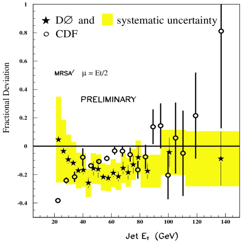
Figure 16: Preliminary DØ and CDF $\mbox{$\sqrt{\rm s}$}=\mbox{630 GeV}$ cross sections compared to NLO QCD predictions. The shaded boxes represent the DØ systematic errors.

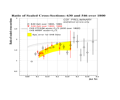
Figure 17: CDF scaling result from Tevatron runs at $\sqrt{\rm s}$= 546 and 1800 GeV in 1989, compared to the preliminary result from the Run 1B runs at 630 GeV and 1800 GeV.

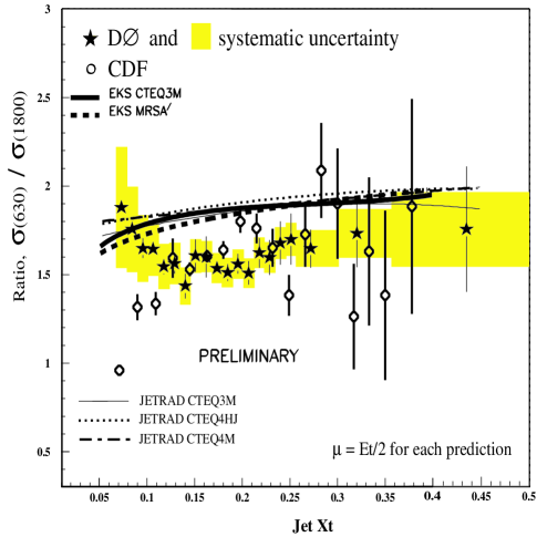
Figure 18: Preliminary DØ and CDF cross section ratios for $\mbox{$\sqrt{\rm s}$}=\mbox{630 GeV}$ to $\mbox{$\sqrt{\rm s}$}=\mbox{1800 TeV}$ compared to NLO QCD predictions. The shaded boxes represent the DØ systematic errors.

6 DIJET DIFFERENTIAL CROSS SECTIONS AT LARGE RAPIDITY

6.1 Introduction

Measurements of the dijet differential cross sections in different rapidity regions can provide additional information and constraints on the QCD predictions. By restricting the $E_{T}$ and rapidity of the leading two jets in the events, different regions of $x$ and $Q^{2}$ can be probed. This may permit a more direct measure of the proton PDFs at Tevatron energies. For instance at LO, an $E_{T}$ = 90 GeV, $\eta=0$ ($\theta$=90^o) jet must be balanced by a second $E_{T}$ = 90 GeV jet. If the second jet is at $\eta=0$, both jet energies equal 90 GeV and so $x_{1}=x_{2}=0.10$. However if the second jet is more forward, since $E_{T}=E\sin\theta$ and $\sin\theta$ is smaller, the jet energy and its fraction of the initial hadronic momentum must increase to maintain $E_{T}$ = 90 GeV. At LO the parton momentum fraction $x$ is related to the $E_{T}$ and $\eta$ of the two jets by the equations:

$$x_{1}=\frac{E_{T}}{\sqrt{s}}({\rm e}^{\eta_{1}}+{\rm e}^{\eta_{2}}),\;\;\;\;x_{2}=\frac{E_{T}}{\sqrt{s}}({\rm e}^{-\eta_{1}}+{\rm e}^{-\eta_{2}}).$$

For $E_{T}$ = 90 GeV jets at $\eta=0$ and $2$, $x=0.06$ and $0.42$. For multi–jet production the calculations of $x$ are generalized to

$$x_{1}=\frac{1}{\sqrt{s}}\sum_{i}E_{Ti}{\rm e}^{\eta_{i}},\;\;\;\;x_{2}=\frac{1}{\sqrt{s}}\sum_{i}E_{Ti}{\rm e}^{-\eta_{i}}.$$

where “$i$” runs over all jets in an event.

Experimentally, the differential dijet cross sections are most conveniently given by

$$\frac{d^{3}\sigma}{d\mbox{$E_{T}$}d\eta_{1}d\eta_{2}},$$

where $\eta_{1}$ and $\eta_{2}$ are the pseudorapidities of the leading two jets. As with the inclusive cross section, the dijet differential cross sections are integrated over a range of pseudorapidity. The cross sections are also integrated over a range of $E_{T}$, but here there is even more freedom in the definition of $E_{T}$: the leading jet $E_{T}$ , the average of the leading two jet $E_{T}$’s, or both leading jet $E_{T}$’s (two entries into the cross section, one for the $E_{T}$ of each of the leading two jets). The specific choice depends upon the experimental conditions. Although they are still preliminary we present the dijet differential cross sections here in order to demonstrate the potential and strength of these measurements. Once the systematic uncertainties are well understood these measurements will strongly constrain the PDFs.

6.2 The CDF Measurement

In the CDF Run 1B measurement, the two highest $E_{T}$ jets are identified and one is required to be in the central (0.1$\leq|\eta|\leq$0.7) region. Because the central region has the smallest energy scale uncertainty, the central jet is used to measure the $E_{T}$ of the event. The other jet, called the “probe” jet, is required to have $E_{T}>$10 GeV and to fall in one of the $\eta$ bins: 0.1$\leq|\eta|\leq$0.7, 0.7$\leq|\eta|\leq$1.4, 1.4$\leq|\eta|\leq$2.1, 2.1$\leq|\eta|\leq$3.0. There are no restrictions on the presence of additional jets. Figure 19 shows the preliminary cross section [47] in the individual $\eta$ bins as a function of the central jet $E_{T}$. JETRAD is used for the theoretical predictions with scale $\mu$ = 0.5 $E_{T}^{max}$ and $R_{sep}$=1.3. The data are compared to the predictions using three parton distribution functions, CTEQ4HJ, MRST and CTEQ4M. The statistical uncertainty is shown on the points. Figure 20 shows the percent difference between the data and theory (CTEQ4M) as a function of the central jet $E_{T}$ for each rapidity bin. The additional curves represent the percent difference from the prediction using CTEQ4M for predictions using MRST and CTEQ4HJ. The systematic uncertainty on the measurement is evaluated in a manner similar to the inclusive jet cross section. The quadrature sum of the systematic uncertainties is shown in the box below the points. The high rapidity bins reach $x$ of roughly 0.6–0.7, while the $E_{T}$ of the jets is in the 100 – 200 GeV range. The excess over predictions using CTEQ4M observed in the inclusive cross section at high $E_{T}$ is seen in all four rapidity bins. This suggests that it is not a function of the jet $E_{T}$, but rather a function of $x$ and is thus related to inadequacies in the PDFs. The improved agreement in all bins when CTEQ4HJ is used is similarly suggestive.

Figure 19: CDF cross sections for central jets with the second jet in different rapidity intervals.

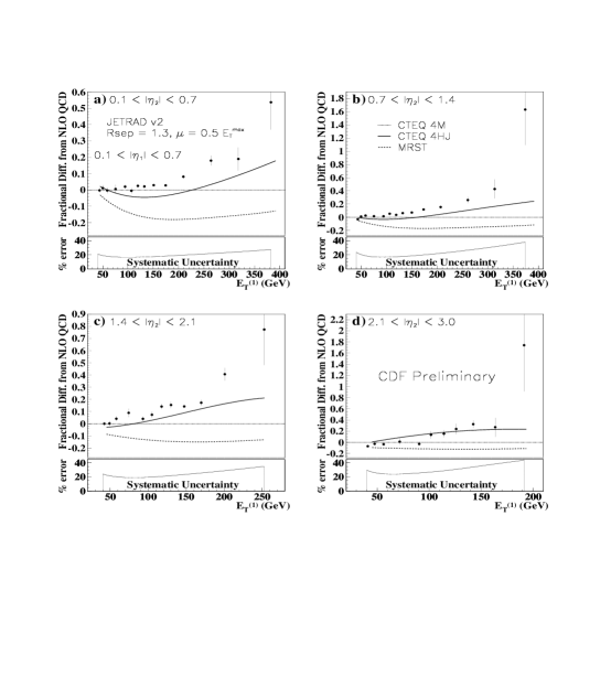
Figure 20: Percent difference between preliminary CDF data (points) and a NLO QCD prediction using the JETRAD program, CTEQ4M, $R_{sep}$=1.3 and $\mu$=$E_{T}^{max}/2$. The percent difference between predictions using CTEQ4M and predictions using MRST and CTEQ4HJ are also shown. The four plots represent the cross section as a function of the central jet $E_{T}$ when the rapidity of the second jet is restricted to different ranges. The curve in the lower box represents the quadrature sum of the correlated systematic uncertainties.

6.3 The D0 Measurement

The D0 Run 1B (92 $pb^{-1}$) measurement organizes the dijet differential cross section according to the rapidity of both leading jets. The rapidities are divided into four same–side (SS) bins where $\eta_{1}\sim\eta_{2}$ and four opposite–side (OS) bins where $\eta_{1}\sim-\eta_{2}$. The bins and approximated $x$ ranges sampled (assuming a L0 process and the observed $E_{T}$ ranges in each bin) are listed in Table 3. The eight cross sections are all plotted versus jet $E_{T}$. Here each event has two entries, one for the $E_{T}$ of each of the leading two jets. As indicated in the table, the low rapidity measurements can provide confirmation of previous PDF measurements extrapolated from low $Q^{2}$. On the other hand, the large rapidity, SS events probe much larger $x$ values.

Table 3: $x$ ranges of SS and OS dijet differential cross sections.

$\eta$ bin	Topology	$x_{min}$	$x_{max}$
0.0-0.5	SS	0.04	0.53
0.0-0.5	OS	0.07	0.42
0.5-1.0	SS	0.03	0.73
0.5-1.0	OS	0.08	0.45
1.0-1.5	SS	0.02	0.81
1.0-1.5	OS	0.10	0.44
1.5-2.0	SS	0.01	0.80
1.5-2.0	OS	0.16	0.46

The D0 analysis follows the inclusive analysis very closely. Jet and event selection, energy correction, and resolution unsmearing are all quite similar. An additional correction for vertex resolution is also important in the very forward–backward rapidity bins. The cross section uncertainties are quite similar to the inclusive cross section for the four rapidity bins limited by $\eta=1.0$. In the high $\eta$ bins the systematic errors are approximately doubled. Figs. 21 and 22 show the fractional difference between data and theory for all eight bins [47, 50]. The theoretical prediction is from JETRAD with CTEQ3M and $\mu=0.5E_{T}^{max}$. The bars on the data represent the statistical uncertainty and the outer symbols the total uncertainty. Note there is good agreement over all rapidity for $x=0.01$ to $0.80$. Significantly, this PDF includes no collider jet data. Although not shown, the agreement with CTEQ4M is also reasonable.

Figure 21: D0 same–side and opposite–side cross sections compared to JETRAD with $R_{sep}$=1.3, $\mu=E_{T}^{max}/2$ and CTEQ3M. The two leading jets are restricted to different $\eta$ regions. See the text for details.

Figure 22: D0 same–side and opposite–side cross sections compared to JETRAD with $R_{sep}$=1.3, $\mu=E_{T}^{max}/2$ and CTEQ3M. The two leading jets are restricted to different $\eta$ regions. See the text for details.

6.4 Prospects

The differential cross sections show great promise for constraining the PDFs. In all rapidity bins the CDF data appears to prefer CTEQ4HJ over CTEQ4M or MRST, while the D0 data seems to be good agreement with the predictions using CTEQ3M. This apparent disagreement mirrors the situation in the inclusive cross sections. However, a firm statement on the agreement or disagreement of the two data sets is obscured by the different techniques and the current lack of quantitative comparisons between data and theory.

7 DIJET MASS AND ANGULAR DISTRIBUTIONS AT 1800 TEV

7.1 Introduction

The LO cross section for $p\bar{p}\rightarrow$ $jet_{1}$ + $jet_{2}$ + $X$ events (where $jet_{1}$ and $jet_{2}$ are the leading two jets) can be completely described in terms of three orthogonal center–of–mass variables. These are cos $\theta^{*}$, where $\theta^{*}$ is the center–of–mass scattering angle between the two leading jets, the boost of the dijet system $\eta_{boost}=(\eta_{1}+\eta_{2})/2$, and the dijet mass, $M_{jj}$ as follows [51]:

$$\frac{d^{3}\sigma}{d\eta_{boost}dM_{jj}dcos\theta^{*}}=\frac{\pi\alpha_{s}^{2}(Q^{2})}{2s^{2}}(2M_{jj})\sum_{1,2}\frac{f(x_{1},Q^{2})}{x_{1}}\frac{f(x_{2},Q^{2})}{x_{2}}|m_{12}|^{2},$$

where $\alpha_{s}^{2}(Q^{2})$ is the strong coupling strength, $|m_{12}|^{2}$ is the hard scattering matrix element, $x_{1}$ ($x_{2}$) is the fraction of the proton (antiproton) momentum carried by the parton and $f(x_{1},Q^{2})$ is the parton momentum distribution. Typically the dijet mass is derived from measured variables such as $E_{T}$ , $\eta_{jet}$, and $\phi_{jet}$. In the case of higher order processes, where more than two jets are produced, the mass is calculated using the two highest $E_{T}$ jets in the event and additional jets are ignored.

Integration of the general dijet cross section over boost and production angle leads to the dijet mass spectrum. The spectrum is a useful test of QCD sensitive to the PDFs. On the other hand integration over mass and boost leads to the dijet angular distribution – a marvelous test of the hard scattering matrix elements almost totally insensitive to the PDFs. Comparisons of the angular distributions and certain mass spectra ratios to theoretical predictions can establish stringent limits on the presence of conjectured quark constituents. We turn now to a discussion of the these spectra and compositeness limits.

7.2 The Mass Distributions

At LO, where only two jets are produced, the dijet invariant mass is given by

$$M_{jj}^{2}=\hat{s}=x_{1}x_{2}s$$

where $\hat{s}$ is the center of mass energy of the interacting partons and $s$ the total center–of–mass energy. Since the dijet mass represents the center–of–mass energy of the interaction it directly probes the parton distribution functions. Experimentally, the dijet mass cross section is given by

$$\frac{d^{3}\sigma}{dM_{jj}d\eta_{1}d\eta_{2}},$$

where $\eta_{1}$ and $\eta_{2}$ are the pseudorapidities of the jets. As with the inclusive jet cross section the dijet mass cross section is integrated over a range of pseudorapidity. For example, Fig. 23 shows NLO QCD dijet predictions for $|\eta_{jet}|\leq 1.0$ relative to a reference prediction. There are 20–30% variations due to the scale and to the PDFs.

Figure 23: The difference between alternative predictions and the reference prediction ($\mu=0.5E^{max}_{T}$, CTEQ3M) for the inclusive dijet mass cross section at $\sqrt{\rm s}$= 1800 GeV for $\eta_{jet}\leq 1.0$. The alternative predictions are for (a) $\mu$ = 0.25, 0.75, 1.0 and 2.0 $\times E^{max}_{T}$, (b) $\mu$ = 0.25, 0.5, and 1.0 $\times\mbox{$\sqrt{\rm s}$}$, (c) CTEQ4M, CTEQ4HJ, MRS(A)́, and MRST, and (d) calculations with the CTEQ4A series of PDFs (which vary $\alpha_{s}$) compared with the calculation using CTEQ4M.

The D0 and CDF collaborations have both measured the dijet mass spectrum with Run 1B data samples. The CDF measurement uses the four–vector definition for the dijet mass $M_{jj}=\sqrt{(E_{1}+E_{2})^{2}-(P_{1}+P_{2})^{2}}$ where $E$ and $P$ are the energy and momentum of a jet and allows the rapidity of the jets to extend to $|\eta_{jet}|<2.0$. To ensure good acceptance, the CDF analysis also imposes a cut on $|cos\theta^{*}|<2/3$, where $\theta^{*}$ is the scattering angle in the center–of–mass frame. Figure 24 shows the CDF preliminary data compared to JETRAD predictions [47]. The error bars represent the quadrature sum of the statistical and systematic uncertainties. The data and JETRAD predictions using CTEQ4M, $\mu=0.5E_{T}^{jet}$ and $R_{sep}=1.3$ are in good agreement. Figure 25 shows the percent difference between the data and the theoretical prediction. The shaded band shows the preliminary estimate of the systematic uncertainties. These uncertainties are derived in a manner similar to the inclusive jet cross section measurement with additional contributions for jets outside the central region. The percent difference between the default prediction and those using other PDFs are also shown and are all consistent with the data given the systematic errors. However, as with the inclusive and dijet cross section measurements, CTEQ4HJ seems to provide the best agreement with the data in the high $E_{T}$ region.

Figure 24: Dijet mass as measured by CDF compared to the NLO prediction from JETRAD with CTEQ4M and $\mu=E_{T}^{max}/2$ and $R_{sep}$=1.3. The error bars indicate the quadrature sum of the statistical and systematic uncertainties

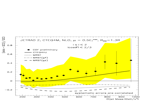
Figure 25: CDF data compared to predictions from the JETRAD program for CTEQ4M and $\mu=E_{T}^{max}/2$ and $R_{sep}$=1.3 (full circles). Predictions using other PDFs and $\mu=E_{T}^{max}/2$ are also compared to CTEQ4M: MRST (dotted), CTEQ4M with $\mu=E_{T}^{max}$ (dashed), and CTEQ4HJ (solid). The error bars indicate the statistical errors. The shaded area represents the combined systematic uncertainty.

D0 has performed the dijet mass measurement in two rapidity regions: central, $|\eta_{jet}|<0.5$, and more forward, $|\eta_{jet}|<1.0$, $|\Delta\eta_{jet}|<1.6$ [52]. The dijet mass at D0 is defined assuming massless jets: $M_{jj}=\sqrt{2E_{T}^{1}E_{T}^{2}(cosh(\Delta\eta)-cos(\Delta\phi))}$, where $\Delta\eta$ and $\Delta\phi$ are the rapidity and azimuthal separation of the two jets. Figure 26 shows the difference between the data and theory divided by the theory. As with the D0 inclusive jet measurement there is good agreement with theory, well within systematic uncertainties. At larger rapidity the data shows a tendency to be slightly above the predictions at high $E_{T}$. Data–theory $\chi^{2}$ comparisons similar to those described in Section 4 yield large probabilities. As Fig. 27 illustrates there is sensitivity to the PDF choice but unfortunately its significance is obscured by the systematic uncertainties. As with the inclusive jet cross section these uncertainties are highly correlated. In Fig. 28, the D0 $\mbox{$|\eta|$}\leq 1.0$ result is compared to the CDF result and to predictions with CTEQ4M. The kinematic cuts of the two analyses have a significant overlap; 59% of the CDF sample has the two leading jets within $\mbox{$|\eta|$}\leq 1.0$. There is remarkable agreement between these data samples over the full $E_{T}$ range.

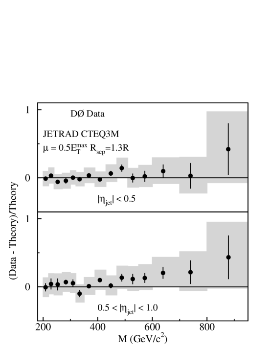
Figure 26: The difference between the D0 dijet mass data and the prediction (JETRAD ) divided by the prediction for $|\eta_{jet}|\leq 0.5$ and $0.5<|\eta_{jet}|<1.0$. The solid circles represent the comparison to the calculation using CTEQ3M with $\mu=0.5\mbox{$E_{T}$}^{max}$. The shaded region represents the $\pm$$1\sigma$ systematic uncertainties.

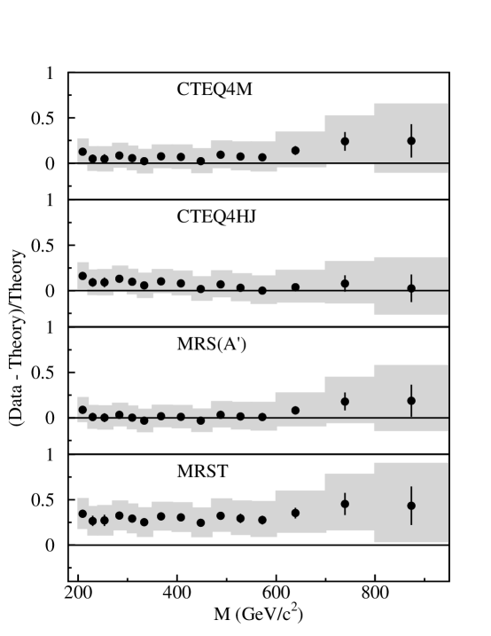
Figure 27: For $|\eta_{jet}|<$1.0, the difference between the D0 dijet mass data and JETRAD predictions divided by the predictions. The calculations used $\mu=0.5\mbox{$E_{T}$}^{max}$, $R_{sep}$=1.3 and CTEQ4M, CTEQ4HJ, MRS(A^′), and MRST. The error bars represent the statistical uncertainty on the data. The shaded region represents the $\pm 1\sigma$ systematic uncertainties

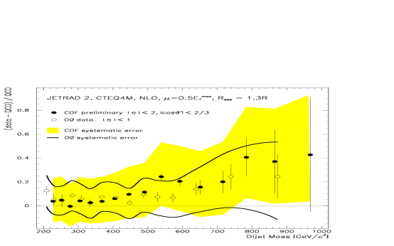
Figure 28: D0 (open circles) and preliminary CDF (full circles) dijet mass results compared to predictions from the JETRAD program for CTEQ4M and $\mu=E_{T}/2$.

7.3 The Dijet Angular Distributions

The dijet angular distribution measured in the center–of–mass is sensitive primarily to the hard scattering matrix elements. In fact, the distribution is unique among high $E_{T}$ measurements in that it is almost independent of the PDFs. The shape of the angular distribution is dominated by t–channel exchange and is nearly identical for all dominant scattering subprocesses (e.g. $gg\rightarrow gg$, $qg\rightarrow qg$, and $qq\rightarrow qq$). The dijet angular distribution predicted by LO QCD (two jets only) is proportional to the Rutherford cross section

$$\frac{d\sigma}{dcos\theta^{*}}\propto\frac{1}{sin^{4}(\theta^{*}/2)}.$$

To flatten out the distribution and facilitate the comparison to theory, the variable transformation $\chi=\frac{1+|cos\theta^{*}|}{1-|cos\theta^{*}|}$ is used giving

$$\frac{d^{3}\sigma}{dM_{jj}d\chi d\eta_{boost}}.$$

For measurement of the dijet angular spectra this quantity is integrated over pseudorapidity and mass regions and normalized to the total number of events N in those regions. The normalization reduces both experimental and theoretical uncertainties. Figure 29 shows the $\frac{1}{N}\frac{dN}{d\chi}$ distributions from the D0 collaboration for four mass ranges [53]. In all cases the jets are limited to regions of full acceptance. The NLO predictions from JETRAD with $\mu=E_{T}^{max}$ provide the best agreement with the shape of the data. The large $\chi$ acceptance of the measurement allows discrimination between LO and NLO predictions. Figure 30 shows CDF data compared to QCD predictions (JETRAD ) for different mass bins [54]. In this case both LO and NLO QCD are in good agreement with the distribution.

Figure 29: Dijet angular distribution as measured by D0 for different mass ranges compared to LO and NLO QCD predictions.

Figure 30: Dijet angular distribution as measured by CDF for different mass ranges compared to LO and NLO QCD predictions.

7.4 Compositeness and New Physics Limits

The dijet mass and angular distributions are sensitive to new physics such as quark compositeness. In QCD parton–parton scattering, the dominant exchange involves the t–channel. This produces distributions peaked at small center–of–mass scattering angles (near the beam axis in the lab) e.g. large $\eta$ and $\chi$. In contrast, the compositeness model [11] predicts a more isotropic angular distribution. Thus, relative to QCD predictions, the contributions of composite quarks would be most noticeable in the central region, near $\eta=0$ and $\chi$ = 1.

Compositeness signals may be parameterized by a mass scale $\Lambda$ which characterizes the quark–substructure coupling. Limits on $\Lambda$ are set assuming that $\Lambda\gg\sqrt{\rm\hat{s}}$, such that the dominant force is still QCD. The substructure coupling is approximated by a four–Fermi contact interaction giving rise to an effective Lagrangian [11]. The Lagrangian contains eight terms describing the coupling of left and right handed quarks and antiquarks. Currently only the term describing the left handed coupling of quarks and anti–quarks has been calculated, and this term has an unknown phase. Limits are reported for the case where specific quarks or all quarks are composite with either constructive interference ($\Lambda^{-}$) or destructive interference ($\Lambda^{+}$). To set compositeness limits CDF and D0 both use the NLO JETRAD prediction times a “k–factor” from LO QCD + compositeness  [54]. NLO calculations with compositeness are not available. Figure 30 includes a curve with a compositeness signal added. The additional contribution at low $\chi$ is most pronounced in the highest dijet mass bins.

Both CDF and D0 set compositeness limits based on the ratio of number of events at low $\chi$ to those in the high $\chi$ region. Figure 31 shows the CDF result for the ratio of the number of events below $\chi$=2.5 and between $\chi$= 2.5 and 5.0 as a function of the dijet mass, along with curves which correspond to the different values of $\Lambda$. Using this ratio, the CDF data excludes at the 95% C.L. a contact interaction scale of $\Lambda^{+}_{ud}\leq 1.6$ TeV and $\Lambda^{-}_{ud}\leq 1.4$ TeV. For a model where all quarks are composite $\Lambda^{+}\leq 1.8$ TeV and $\Lambda^{-}\leq 1.6$ TeV. Figure 32 shows the angular distribution as measured by D0 for very high dijet masses (greater than 635 GeV/c²) compared to predictions which include composite quarks. Compositeness limits in this analysis are derived from the ratio of the number of events above and below $\chi$=4. The data excludes (at the 95% CL) contact interaction scales with $\mu=1.0E_{T}^{max}$: $\Lambda^{-}_{ud}\leq 2.0$ TeV, $\Lambda^{-}\leq 2.2$ TeV, $\Lambda^{+}\leq 2.1$ TeV, and with $\mu=0.5E_{T}^{max}$: $\Lambda^{-}_{ud}\leq 2.2$ TeV, $\Lambda^{-}\leq 2.4$ TeV, $\Lambda^{+}\leq 2.3$ TeV.

Figure 31: Dijet angular distribution as measured by CDF compared to QCD and to QCD plus a term for composite quarks. Limits on compositeness are derived from the dijet angular distribution ratio of the number events below $\chi$=2.5 to the number between 2.5 and 5.

Figure 32: Dijet angular distribution as measured by D0 compared to predictions with additional contributions from composite quarks.

The best limits on compositeness now come from recent dijet mass measurements from the D0 collaboration [52] which combine the sensitivity of the dijet mass distributions with the PDF independence of the angular distributions. In much the same way jet production from a composite interaction increases the $\chi$ spectrum at low values of $\chi$, the dijet mass spectrum will increase at central rapidities relative to forward rapidities. Thus the ratio of the central and forward dijet mass spectra will be sensitive to $\Lambda$. In addition, both theoretical and experimental uncertainty are reduced in the ratio. Fig. 33 shows the ratio of cross–sections for $|\eta_{jet}|\leq 0.5$ and $0.5\leq|\eta_{jet}|\leq 1.0$ as a function of dijet mass. As indicated by the family of curves, the compositeness model predicts changes in shape to this ratio at high mass. The spectrum rules out quark compositeness at the 95% confidence level for $\Lambda^{+}$ below $2.7$ TeV and $\Lambda^{-}$ below $2.5$ TeV.

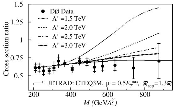
Figure 33: The ratio of D0 dijet mass cross sections for $|\eta_{jet}|<0.5$ and $0.5<|\eta_{jet}|<1.0$ for data (solid circles) and theory (various lines). The error bars show the statistical and systematic uncertainties added in quadrature, and the crossbar shows the size of the statistical error.

8 CONCLUSIONS

The inclusive jet and dijet cross sections provide fundamental tests of QCD predictions at the highest jet $E_{T}$ and thus are the deepest probes into the structure of the proton. With the increased luminosity performance of the Tevatron, measurements of these cross sections are no longer limited by statistical uncertainties. In fact, the systematic uncertainties from the experimental measurements and from the theoretical predictions are comparable in size and are significantly larger than the statistical uncertainty on all but the highest $E_{T}$ data points. Uncertainties in the PDFs dominate the theoretical uncertainty, while uncertainties in the jet energy scale dominate the experimental measurements.

The inclusive jet cross sections from the Tevatron have proved a particularly interesting test of QCD. The Run 1A inclusive jet measurement showed disagreement with concurrent pQCD predictions at the highest $x$ and $Q$. Two subsequent measurements, each using five times the data, show mixed agreement between the data and theory at high $E_{T}$. One measurement is consistent with the Run 1A measurement, and can be described by QCD if the PDFs are suitably modified. The second Run 1B measurement is well described by QCD with PDFs that either do or do not include high $E_{T}$ jet data. Further, within statistical and systematic errors, the three measurements are compatible. The preliminary measurements of the inclusive jet cross section at $\sqrt{s}$=630 GeV and the ratio of the cross sections show good agreement with previous results and marginal agreement with QCD predictions. Derivation of quantitative results is in progress. Unfortunately this sample is too statistically limited to provide a constraint on the high $E_{T}$ behavior of the cross section at 1800 GeV.

The apparent excess of events at high $E_{T}$ observed in the inclusive jet cross section from Run 1A created intense scrutiny of the theoretical predictions. As a result, there is now a better understanding of the uncertainty in the theoretical predictions, particularly for the parton distribution functions. The dijet mass distributions and differential cross sections reflect a story similar to the inclusive jet measurements. The results are generally consistent with each other and with QCD, but with hints that moderately forward regions indicate some high $x$ modifications of the PDFs might be appropriate. Incorporation of this information into the global fitting procedures used to derive the PDFs should be particularly helpful in reducing the uncertainty associated with extrapolation from low energy DIS data to the kinematic region covered by the Tevatron jet measurements.

Until the uncertainty in the PDFs is reduced, or a method of analytically evaluating their uncertainties is available, the best limits on compositeness will come from measurements insensitive to the PDFs, and in particular, measurements that rely on angular information. These angular distributions show the partonic hard scattering to be well described by NLO theoretical calculations. Comparisons of the angular and mass data to jet production models augmented by quark compositeness show no preference for deviations from standard QCD predictions. In fact, the analyses now show that the compositeness scale must be greater than 2.5 TeV if it exists at all.

The high precision Tevatron jet data has fostered a period of great progress in QCD. Due to the flexibility of theoretical predictions, pQCD can describe nearly all inclusive jet and dijet observations. Limits on quark substructure from Run 1 have nearly doubled from the previous measurements. However, more stringent tests will require improved PDFs and reduced theoretical uncertainties. Looking forward, expectations are high that the experimental measurements of jets and their properties will continue to improve in Run 2 with a 20–fold increase in data sample size, increased beam energy, and reduced systematic uncertainties from the upgraded detectors.

ACKNOWLEDGMENTS

We wish to thank the members of the CDF and D0 Collaborations for permitting us to include their results; in particular we would like to thank Iain Bertrum, Anwar Bhatti, Frank Chlebana, Bjoern Hinrichsen, Bob Hirosky and John Krane for helpful discussions during preparation of this review and for providing excellent illustrations.

References

- 1. T. Akesson et al., (AFS Collaboration), Phys. Lett. B123, 133 (1983).
- 2. J. Appel et al., (UA2 Collaboration), Phys. Lett. B160, 349 (1985); J. Alitti et al. (UA2 Collaboration), Phys. Lett. B257, 232 (1991)
- 3. G. Arnison et al., (UA1 Collaboration), Phys. Lett. B172, 461 (1986).
- 4. F. Abe et al., (CDF Collaboration), Phys. Rev. Lett. 62, 613 (1989).
- 5. F. Abe et al., (CDF Collaboration), Phys. Rev. Lett. 68, 1104 (1992).
- 6. C. Albajar et al., (UA1 Collaboration), Phys. Lett. B209, 127 (1988).
- 7. J. Alitti et al., (UA2 Collaboration), Zeit. Phys.. B49, 17 (1991).
- 8. F. Abe et al., (CDF Collaboration), Phys. Rev. Lett. 71, 2542 (1993).
- 9. F. Abe et al., (CDF Collaboration), Phys. Rev. Lett. 62, 3020 (1989).
- 10. F. Abe et al., (CDF Collaboration), Phys. Rev. Lett. 69, 2896 (1992).
- 11. E. Eichten, K. Lane and M. Peskin, Phys. Rev. Lett 50, 811 (1983).
- 12. E. Huth and M. .L Mangano, ”QCD Tests in Proton–Antiproton Collisions”, Annu. Rev. Nucl. Part. Sci. 43 585 (1993).
- 13. F. Abe et al., (CDF Collaboration), Phys. Rev. Lett. 77, 438 (1996).
- 14. D. Soper, Talk given at the 28th International Conference on High Energy Physics, Warsaw, Poland, Jul 1996, hep–ph/9610434, OITS–619.
- 15. W. J. Stirling, in Proceedings of the 17th International Conference on Physics in Collision, Bristol, England, 1997. p243.
- 16. B. Abbott et al., Eur. Phys. J. C 5, 687 (1998).
- 17. See for example J. Huston (for the CDF Collaboration) FERMILAB–CONF–99–006–E, to be published in the proceedings of 29th International Conference on High–Energy Physics (ICHEP 98), Vancouver, Canada, 23–29 Jul 1998.
- 18. B. Abbott et al., (D0 Collaboration), Accepted by Phys. Rev. Lett. Preprint hep–ph/9807018.
- 19. R. K. Ellis, W. J. Stirling, and B. R. Webber, QCD and Collider Physics; Cambridge Univ. Press (1996); p238.
- 20. S. D. Ellis, Z. Kunszt, and D. E. Soper, Phys. Rev. Lett. 64, 2121 (1990).
- 21. F. Aversa et al., Phys. Rev. Lett. 65, 401 (1990).
- 22. W. T. Giele, E. W. N. Glover, and D. A. Kosower, Phys. Rev. Lett. 73,2019 (1994).
- 23. See http://zebu.uoregon.edu/ soper/EKSJets/jet.html.
- 24. See http://www-theory.fnal.gov/people/giele/giele.html.
- 25. J. Huth et al. “Proceedings 1990 Summer Study on High Energy Physics, ed. E Berger. Singapore: World Scientific, 134 (1992).
- 26. S.K. Ellis, Z. Kunszt, D. Soper, Phys. Rev. Lett. 69 3615 (1992) and S. Ellis CERN–TH–6861–93, Jun 1993. 13pp. Presented at 28th Rencontres de Moriond: QCD and High Energy Hadronic Interactions, Les Arcs, France, 20–27 Mar 1993. Published in Moriond 1993: Hadronic:235–244; hep–ph/9306280.
- 27. B. Abbott et al., Fermilab–Pub–97–242–E (1997).
- 28. J. Botts et al., CTEQ Collaboration, Phys. Lett. B304 159 (1993).
- 29. H. L. Lai et al., Phys. Rev. D 51, 4763 (1995).
- 30. A. D. Martin, R. G. Roberts and W. J. Stirling, Phys. Lett. B354, 154 (1995).
- 31. H. L. Lai et al., Phys. Rev. D 55, 1280 (1997).
- 32. A. D. Martin et al., hep–ph/9803445, Eur. Phys. J. C C 4, 463 (1998)
- 33. J. Huston et al. Phys.Rev. D58 114034 (1998), hep–ph/9801444.
- 34. U.K Yang, A. Bodek, Talk given at 29th International Conference on High–Energy Physics (ICHEP 98), Vancouver, Canada, 23–29 Jul (1998), hep–ph/9809480.
- 35. F. Abe et al. (CDF Collaboration) NIM Res., Sect. A271, 387 (1988) and references therein. F. Abe et al. (CDF Collaboration) Phys.Rev.D50 2966 (1994).
- 36. S. Abachi et al. (DØCollaboration), “The D0 Detector”, NIM A338 185 (1994).
- 37. M. Albrow, et al. CDF NOTE 4844, FERMILAB-TM-2071 (1999).
- 38. F. Abe et al. (CDF Collaboration) Phys. Rev. D50 5550, (1994).
- 39. J. Bantly, et al. FERMILAB–TM–1930, Mar. (1996).
- 40. B. Abbott et al., Accepted by Nucl. Instr. and Meth. A, hep–ex/9805009 (1998).
- 41. M. Bhattacharjee, Ph. D. Thesis, University of Delhi, India, unpublished(1996).
- 42. C. Haber et al. Nucl.Instrum.Meth. A289 388 (1990).
- 43. F. Abe et al. (CDF Collaboration) Phys.Rev.D47 4857 (1993).
- 44. F. Abe et al., (CDF Collaboration), Phys. Rev. D 45, 1448 (1992).
- 45. F. Abe (CDF Collaboration) et el., Phys. Rev. Lett. 70 1376 (1993) .
- 46. F. Abe et al. (CDF Collaboration) FERMILAB–PUB–98/280–E, submitted to PRD.
- 47. B. Hirosky and F. Bedeschi in the Proceedings of the Hadron Collider Physics Workshop XIII, Jan. 14–20, 1999, Bombay, India.
- 48. J. Huston in the Proceedings of the 29th International Conference on High–Energy Physics (ICHEP 98), Vancouver, Canada, 23–29 July 1998. MSUHEP–90119, hep–ph/9901352.
- 49. G. Blazey in the Proceedings of the 29th International Conference on High–Energy Physics (ICHEP 98), Vancouver, Canada, 23–29 July 1998. FNAL–98–367–E. J. Krane, unpublished theses University of Nebraska, Lincoln (1998).
- 50. G. DiLoretto, Ph. D. Thesis, Michigan State University, East Lansing, Michigan, unpublished (1998).
- 51. R.K. Ellis and J. Sexton, Nucl., Phys. B269 445 (1986).
- 52. B. Abbott et al. (D0 Coll.), Phys. Rev. Lett. Accepted for publication (1999).
- 53. B. Abbott et al. (D0 Coll.), Phys. Rev. Lett. 80, 666 (1998).
- 54. CDF Collaboration, F. Abe et el., Phys. Rev. Lett. 77 5336(1996); Erratum–ibid.78 4307 (1997).