DESY 99-010                                                                           ISSN 0418-9833
February 1999

Elastic Electroproduction of $\rho$ Mesons
at HERA

H1 Collaboration

The elastic electroproduction of $\rho$ mesons is studied at HERA with the H1 detector for a photon virtuality in the range $1<Q^{2}<60~{}{\rm GeV^{2}}$ and for a hadronic centre of mass energy in the range $30<W<140$ GeV. The shape of the ($\pi\pi$) mass distribution in the $\rho$ resonance region is measured as a function of $Q^{2}$. The full set of $\rho$ spin density matrix elements is determined, and evidence is found for a helicity flip amplitude at the level of $8\pm 3\%$ of the non-flip amplitudes. Measurements are presented of the dependence of the cross section on $Q^{2}$, $W$ and $t$ (the four-momentum transfer squared to the proton). They suggest that, especially at large $Q^{2}$, the $\gamma^{*}p$ cross section develops a stronger $W$ dependence than that expected from the behaviour of elastic and total hadron$-$hadron cross sections.

To be submitted to Eur. Phys. J. C.

C. Adloff³⁴, V. Andreev²⁵, B. Andrieu²⁸, V. Arkadov³⁵, A. Astvatsatourov³⁵, I. Ayyaz²⁹, A. Babaev²⁴, J. Bähr³⁵, P. Baranov²⁵, E. Barrelet²⁹, W. Bartel¹¹, U. Bassler²⁹, P. Bate²², A. Beglarian^11,40, O. Behnke¹¹, H.-J. Behrend¹¹, C. Beier¹⁵, A. Belousov²⁵, Ch. Berger¹, G. Bernardi²⁹, T. Berndt¹⁵, G. Bertrand-Coremans⁴, P. Biddulph²², J.C. Bizot²⁷, V. Boudry²⁸, W. Braunschweig¹, V. Brisson²⁷, D.P. Brown²², W. Brückner¹³, P. Bruel²⁸, D. Bruncko¹⁷, J. Bürger¹¹, F.W. Büsser¹², A. Buniatian³², S. Burke¹⁸, A. Burrage¹⁹, G. Buschhorn²⁶, D. Calvet²³, A.J. Campbell¹¹, T. Carli²⁶, E. Chabert²³, M. Charlet⁴, D. Clarke⁵, B. Clerbaux⁴, J.G. Contreras^8,43, C. Cormack¹⁹, J.A. Coughlan⁵, M.-C. Cousinou²³, B.E. Cox²², G. Cozzika¹⁰, J. Cvach³⁰, J.B. Dainton¹⁹, W.D. Dau¹⁶, K. Daum³⁹, M. David¹⁰, M. Davidsson²¹, A. De Roeck¹¹, E.A. De Wolf⁴, B. Delcourt²⁷, R. Demirchyan^11,40, C. Diaconu²³, M. Dirkmann⁸, P. Dixon²⁰, W. Dlugosz⁷, K.T. Donovan²⁰, J.D. Dowell³, A. Droutskoi²⁴, J. Ebert³⁴, G. Eckerlin¹¹, D. Eckstein³⁵, V. Efremenko²⁴, S. Egli³⁷, R. Eichler³⁶, F. Eisele¹⁴, E. Eisenhandler²⁰, E. Elsen¹¹, M. Enzenberger²⁶, M. Erdmann^14,42,f, A.B. Fahr¹², P.J.W. Faulkner³, L. Favart⁴, A. Fedotov²⁴, R. Felst¹¹, J. Feltesse¹⁰, J. Ferencei¹⁷, F. Ferrarotto³², M. Fleischer⁸, G. Flügge², A. Fomenko²⁵, J. Formánek³¹, J.M. Foster²², G. Franke¹¹, E. Gabathuler¹⁹, K. Gabathuler³³, F. Gaede²⁶, J. Garvey³, J. Gassner³³, J. Gayler¹¹, R. Gerhards¹¹, S. Ghazaryan^11,40, A. Glazov³⁵, L. Goerlich⁶, N. Gogitidze²⁵, M. Goldberg²⁹, I. Gorelov²⁴, C. Grab³⁶, H. Grässler², T. Greenshaw¹⁹, R.K. Griffiths²⁰, G. Grindhammer²⁶, T. Hadig¹, D. Haidt¹¹, L. Hajduk⁶, M. Hampel¹, V. Haustein³⁴, W.J. Haynes⁵, B. Heinemann¹¹, G. Heinzelmann¹², R.C.W. Henderson¹⁸, S. Hengstmann³⁷, H. Henschel³⁵, R. Heremans⁴, I. Herynek³⁰, K. Hewitt³, K.H. Hiller³⁵, C.D. Hilton²², J. Hladký³⁰, D. Hoffmann¹¹, R. Horisberger³³, S. Hurling¹¹, M. Ibbotson²², Ç. İşsever⁸, M. Jacquet²⁷, M. Jaffre²⁷, L. Janauschek²⁶, D.M. Jansen¹³, L. Jönsson²¹, D.P. Johnson⁴, M. Jones¹⁹, H. Jung²¹, H.K. Kästli³⁶, M. Kander¹¹, D. Kant²⁰, M. Kapichine⁹, M. Karlsson²¹, O. Karschnik¹², J. Katzy¹¹, O. Kaufmann¹⁴, M. Kausch¹¹, N. Keller¹⁴, I.R. Kenyon³, S. Kermiche²³, C. Keuker¹, C. Kiesling²⁶, M. Klein³⁵, C. Kleinwort¹¹, G. Knies¹¹, J.H. Köhne²⁶, H. Kolanoski³⁸, S.D. Kolya²², V. Korbel¹¹, P. Kostka³⁵, S.K. Kotelnikov²⁵, T. Krämerkämper⁸, M.W. Krasny²⁹, H. Krehbiel¹¹, D. Krücker²⁶, K. Krüger¹¹, A. Küpper³⁴, H. Küster², M. Kuhlen²⁶, T. Kurča³⁵, W. Lachnit¹¹, R. Lahmann¹¹, D. Lamb³, M.P.J. Landon²⁰, W. Lange³⁵, U. Langenegger³⁶, A. Lebedev²⁵, F. Lehner¹¹, V. Lemaitre¹¹, R. Lemrani¹⁰, V. Lendermann⁸, S. Levonian¹¹, M. Lindstroem²¹, G. Lobo²⁷, E. Lobodzinska^6,41, V. Lubimov²⁴, S. Lüders³⁶, D. Lüke^8,11, L. Lytkin¹³, N. Magnussen³⁴, H. Mahlke-Krüger¹¹, N. Malden²², E. Malinovski²⁵, I. Malinovski²⁵, R. Maraček¹⁷, P. Marage⁴, J. Marks¹⁴, R. Marshall²², H.-U. Martyn¹, J. Martyniak⁶, S.J. Maxfield¹⁹, T.R. McMahon¹⁹, A. Mehta⁵, K. Meier¹⁵, P. Merkel¹¹, F. Metlica¹³, A. Meyer¹¹, A. Meyer¹¹, H. Meyer³⁴, J. Meyer¹¹, P.-O. Meyer², S. Mikocki⁶, D. Milstead¹¹, R. Mohr²⁶, S. Mohrdieck¹², M. Mondragon⁸, F. Moreau²⁸, A. Morozov⁹, J.V. Morris⁵, D. Müller³⁷, K. Müller¹¹, P. Murín¹⁷, V. Nagovizin²⁴, B. Naroska¹², J. Naumann⁸, Th. Naumann³⁵, I. Négri²³, P.R. Newman³, H.K. Nguyen²⁹, T.C. Nicholls¹¹, F. Niebergall¹², C. Niebuhr¹¹, Ch. Niedzballa¹, H. Niggli³⁶, O. Nix¹⁵, G. Nowak⁶, T. Nunnemann¹³, H. Oberlack²⁶, J.E. Olsson¹¹, D. Ozerov²⁴, P. Palmen², V. Panassik⁹, C. Pascaud²⁷, S. Passaggio³⁶, G.D. Patel¹⁹, H. Pawletta², E. Perez¹⁰, J.P. Phillips¹⁹, A. Pieuchot¹¹, D. Pitzl³⁶, R. Pöschl⁸, G. Pope⁷, B. Povh¹³, K. Rabbertz¹, J. Rauschenberger¹², P. Reimer³⁰, B. Reisert²⁶, D. Reyna¹¹, H. Rick¹¹, S. Riess¹², E. Rizvi³, P. Robmann³⁷, R. Roosen⁴, K. Rosenbauer¹, A. Rostovtsev^24,12, F. Rouse⁷, C. Royon¹⁰, S. Rusakov²⁵, K. Rybicki⁶, D.P.C. Sankey⁵, P. Schacht²⁶, J. Scheins¹, F.-P. Schilling¹⁴, S. Schleif¹⁵, P. Schleper¹⁴, D. Schmidt³⁴, D. Schmidt¹¹, L. Schoeffel¹⁰, V. Schröder¹¹, H.-C. Schultz-Coulon¹¹, F. Sefkow³⁷, A. Semenov²⁴, V. Shekelyan²⁶, I. Sheviakov²⁵, L.N. Shtarkov²⁵, G. Siegmon¹⁶, Y. Sirois²⁸, T. Sloan¹⁸, P. Smirnov²⁵, M. Smith¹⁹, V. Solochenko²⁴, Y. Soloviev²⁵, V. Spaskov⁹, A. Specka²⁸, H. Spitzer¹², F. Squinabol²⁷, R. Stamen⁸, P. Steffen¹¹, R. Steinberg², J. Steinhart¹², B. Stella³², A. Stellberger¹⁵, J. Stiewe¹⁵, U. Straumann¹⁴, W. Struczinski², J.P. Sutton³, M. Swart¹⁵, S. Tapprogge¹⁵, M. Taševský³⁰, V. Tchernyshov²⁴, S. Tchetchelnitski²⁴, J. Theissen², G. Thompson²⁰, P.D. Thompson³, N. Tobien¹¹, R. Todenhagen¹³, D. Traynor²⁰, P. Truöl³⁷, G. Tsipolitis³⁶, J. Turnau⁶, E. Tzamariudaki²⁶, S. Udluft²⁶, A. Usik²⁵, S. Valkár³¹, A. Valkárová³¹, C. Vallée²³, P. Van Esch⁴, A. Van Haecke¹⁰, P. Van Mechelen⁴, Y. Vazdik²⁵, G. Villet¹⁰, K. Wacker⁸, R. Wallny¹⁴, T. Walter³⁷, B. Waugh²², G. Weber¹², M. Weber¹⁵, D. Wegener⁸, A. Wegner²⁶, T. Wengler¹⁴, M. Werner¹⁴, L.R. West³, G. White¹⁸, S. Wiesand³⁴, T. Wilksen¹¹, S. Willard⁷, M. Winde³⁵, G.-G. Winter¹¹, Ch. Wissing⁸, C. Wittek¹², E. Wittmann¹³, M. Wobisch², H. Wollatz¹¹, E. Wünsch¹¹, J. Žáček³¹, J. Zálešák³¹, Z. Zhang²⁷, A. Zhokin²⁴, P. Zini²⁹, F. Zomer²⁷, J. Zsembery¹⁰ and M. zur Nedden³⁷

¹ I. Physikalisches Institut der RWTH, Aachen, Germany^a
2 III. Physikalisches Institut der RWTH, Aachen, Germany^a
3 School of Physics and Space Research, University of Birmingham, Birmingham, UK^b
4 Inter-University Institute for High Energies ULB-VUB, Brussels; Universitaire Instelling Antwerpen, Wilrijk; Belgium^c
5 Rutherford Appleton Laboratory, Chilton, Didcot, UK^b
6 Institute for Nuclear Physics, Cracow, Poland^d
7 Physics Department and IIRPA, University of California, Davis, California, USA^e
8 Institut für Physik, Universität Dortmund, Dortmund, Germany^a
9 Joint Institute for Nuclear Research, Dubna, Russia
¹⁰ DSM/DAPNIA, CEA/Saclay, Gif-sur-Yvette, France
¹¹ DESY, Hamburg, Germany^a
12 II. Institut für Experimentalphysik, Universität Hamburg, Hamburg, Germany^a
13 Max-Planck-Institut für Kernphysik, Heidelberg, Germany^a
14 Physikalisches Institut, Universität Heidelberg, Heidelberg, Germany^a
15 Institut für Hochenergiephysik, Universität Heidelberg, Heidelberg, Germany^a
16 Institut für experimentelle und angewandte Physik, Universität Kiel, Kiel, Germany^a
17 Institute of Experimental Physics, Slovak Academy of Sciences, Košice, Slovak Republic^f,j
18 School of Physics and Chemistry, University of Lancaster, Lancaster, UK^b
19 Department of Physics, University of Liverpool, Liverpool, UK^b
20 Queen Mary and Westfield College, London, UK^b
21 Physics Department, University of Lund, Lund, Sweden^g
22 Department of Physics and Astronomy, University of Manchester, Manchester, UK^b
23 CPPM, Université d’Aix-Marseille II, IN2P3-CNRS, Marseille, France
²⁴ Institute for Theoretical and Experimental Physics, Moscow, Russia
²⁵ Lebedev Physical Institute, Moscow, Russia^f,k
26 Max-Planck-Institut für Physik, München, Germany^a
27 LAL, Université de Paris-Sud, IN2P3-CNRS, Orsay, France
²⁸ LPNHE, École Polytechnique, IN2P3-CNRS, Palaiseau, France
²⁹ LPNHE, Universités Paris VI and VII, IN2P3-CNRS, Paris, France
³⁰ Institute of Physics, Academy of Sciences of the Czech Republic, Praha, Czech Republic^f,h
31 Nuclear Center, Charles University, Praha, Czech Republic^f,h
32 INFN Roma 1 and Dipartimento di Fisica, Università Roma 3, Roma, Italy
³³ Paul Scherrer Institut, Villigen, Switzerland
³⁴ Fachbereich Physik, Bergische Universität Gesamthochschule Wuppertal, Wuppertal, Germany^a
35 DESY, Institut für Hochenergiephysik, Zeuthen, Germany^a
36 Institut für Teilchenphysik, ETH, Zürich, Switzerland^i
37 Physik-Institut der Universität Zürich, Zürich, Switzerland^i
38 Institut für Physik, Humboldt-Universität, Berlin, Germany^a
39 Rechenzentrum, Bergische Universität Gesamthochschule Wuppertal, Wuppertal, Germany^a
40 Vistor from Yerevan Physics Institute, Armenia
⁴¹ Foundation for Polish Science fellow
⁴² Institut für Experimentelle Kernphysik, Universität Karlsruhe, Karlsruhe, Germany
⁴³ Dept. Fis. Ap. CINVESTAV, Mérida, Yucatán, México

^a Supported by the Bundesministerium für Bildung, Wissenschaft, Forschung und Technologie, FRG, under contract numbers 7AC17P, 7AC47P, 7DO55P, 7HH17I, 7HH27P, 7HD17P, 7HD27P, 7KI17I, 6MP17I and 7WT87P
^b Supported by the UK Particle Physics and Astronomy Research Council, and formerly by the UK Science and Engineering Research Council
^c Supported by FNRS-FWO, IISN-IIKW
^d Partially supported by the Polish State Committee for Scientific Research, grant no. 115/E-343/SPUB/P03/002/97 and grant no. 2P03B 055 13
^e Supported in part by US DOE grant DE F603 91ER40674
^f Supported by the Deutsche Forschungsgemeinschaft
^g Supported by the Swedish Natural Science Research Council
^h Supported by GA ČR grant no. 202/96/0214, GA AV ČR grant no. A1010821 and GA UK grant no. 177
ⁱ Supported by the Swiss National Science Foundation
^j Supported by VEGA SR grant no. 2/5167/98
^k Supported by Russian Foundation for Basic Research grant no. 96-02-00019

1 Introduction

Measurements of the elastic electroproduction of vector mesons at HERA over a wide range of exchanged photon virtuality $Q^{2}$ are of particular interest. For many years it has been known that at low $Q^{2}$, that is with no hard scale, vector meson electroproduction exhibits all the properties of a soft diffractive process. Predictions of soft processes based on QCD calculations are however intractable. The presence of a hard scale, that is a significant $Q^{2}$, makes perturbative QCD calculations possible. Measurements of the $Q^{2}$ dependences of observables in vector meson electroproduction thereby provide insight into the transition and the interplay between soft and hard processes in QCD.

This paper presents an analysis of elastic $\rho$ meson electroproduction:

$$e+p\rightarrow e+\rho+p\ ,\ \ \ \ \rho\rightarrow\pi^{+}+\pi^{-}\ ,$$ (1)

in the $Q^{2}$ range from 1 to 60 ${\rm GeV}^{2}$ ($Q^{2}=-q^{2}$, where $q$ is the four-momentum of the intermediate photon) and the $W$ range from 30 to 140 GeV ($W$ is the hadronic centre of mass energy).

The data were obtained with the H1 detector in two running periods of the HERA collider, operated with 820 GeV protons and 27.5 GeV positrons. A low $Q^{2}$ data set ($1<\mbox{$Q^{2}$}<5$ ${\rm GeV}^{2}$) was obtained from a special run in 1995, with the $ep$ interaction vertex shifted by 70 cm in the outgoing proton beam direction; it corresponds to an integrated luminosity of 125 ${\rm nb^{-1}}$. A larger sample with $2.5<\mbox{$Q^{2}$}<60$ ${\rm GeV}^{2}$ was obtained in 1996 under normal running conditions; it corresponds to a luminosity of 3.87 ${\rm pb^{-1}}$.

The present measurements provide detailed information in the region $1\mathrel{\hbox to0.0pt{\lower 4.0pt\hbox{\hskip 1.0pt$\sim$}\hss}\raise 1.0pt\hbox{$<$}}\mbox{$Q^{2}$}\mathrel{\hbox to0.0pt{\lower 4.0pt\hbox{\hskip 1.0pt$\sim$}\hss}\raise 1.0pt\hbox{$<$}}8$ ${\rm GeV}^{2}$ and they increase the precision of the H1 measurement of $\rho$ electroproduction with $\mbox{$Q^{2}$}>8$ ${\rm GeV}^{2}$, which was first performed using data collected in 1994 [1]. They are compared to results of the ZEUS experiment [2] at HERA and of fixed target experiments [3, 4, 5].

The H1 detector, the definition of the kinematic variables and the event selection are introduced in section 2. Acceptances, efficiencies and background contributions are discussed in section 3. The shape of the ($\pi\pi$) mass distribution and the evolution with $Q^{2}$ of the skewing of this distribution are studied in section 4. Section 5 is devoted to the study of the $\rho$ meson decay angular distributions and to the measurement of the 15 elements of the spin density matrix, as a function of several kinematic variables. The $Q^{2}$ dependence of the ratio $R$ of the longitudinal to transverse $\gamma^{*}p$ cross sections is measured. The violation of $s$-channel helicity conservation, found to be small but significant at lower energies [3, 6], is quantified. Finally, section 6 presents the $t$ distribution and the measurement of the $\gamma^{*}p\rightarrow\mbox{$\rho$}p$ cross section as a function of $Q^{2}$ and $W$. Predictions of several models are compared to the measurements in sections 5 and 6.

2 H1 Detector, Kinematics and Event Selection

Events corresponding to reaction (1) are selected by requiring the detection of the scattered electron and of a pair of oppositely charged particles originating from a common vertex. The absence of additional activity in the detector is required, since the scattered proton generally escapes undetected into the beam pipe.

H1 uses a right-handed coordinate system with the $z$ axis taken along the beam direction, the $+z$ or “forward” direction being that of the outgoing proton beam. The $x$ axis points towards the centre of the HERA ring.

2.1 The H1 Detector

A detailed description of the H1 detector can be found in [7]. Here only the detector components relevant for the present analysis are described.

The scattered electron is detected in the SPACAL [8], a lead – scintillating fibre calorimeter situated in the backward region of the H1 detector, 152 cm from the nominal interaction point. The calorimeter is divided into an electromagnetic and a hadronic part. The electromagnetic section of the SPACAL, which covers the angular range $153^{\rm\circ}<\theta<177.5^{\rm\circ}$ (defined with respect to the nominal interaction point), is segmented into cells of $4\times 4$ $\rm cm^{2}$ transverse size. The hadronic section is used here to prevent hadrons from being misidentified as the scattered electron. In front of the SPACAL, a set of drift chambers, the BDC, allows the reconstruction of electron track segments, providing a resolution in the transverse direction of 0.5 mm.

The pion candidates are detected and their momentum is measured in the central tracking detector. The major components of this detector are two 2 m long coaxial cylindrical drift chambers, the CJC chambers, with wires parallel to the beam direction. The inner and outer radii of the chambers are 203 and 451 mm, and 530 and 844 mm, respectively. In the forward region, the CJC chambers are supplemented by a set of drift chambers with wires perpendicular to the beam direction. The measurement of charged particle transverse momenta is performed in a magnetic field of 1.15 T, uniform over the full tracker volume, generated by a superconducting solenoidal magnet. For charged particles emitted from the nominal vertex with polar angles $20^{\rm\circ}<\theta<160^{\rm\circ}$, the resolution on the transverse momentum is $\Delta p_{t}/p_{t}\simeq\ 0.006\ p_{t}$ (GeV). Drift chambers with wires perpendicular to the beam direction, situated inside the inner CJC and between the two CJC chambers, provide a measurement of $z$ coordinates with a precision of 350 ${\rm\mu m}$.

The ($x,y,z$) position of the interaction vertex is reconstructed for each event by a global fit of all measured charged particle trajectories. For each electron fill in the accelerator, a fit is performed of the dependence on $z$ of the mean $x$ and $y$ positions of the vertices. This provides a measurement of the corresponding beam direction, which varies slightly from fill to fill.

The absence of activity in the H1 detector not associated with the scattered electron or the $\rho$ decay is checked using several components of the detector. The liquid argon (LAr) calorimeter, surrounding the tracking detector and situated inside the solenoidal magnet, covers the polar angular range $4^{\rm\circ}\leq\theta\leq 154^{\rm\circ}$ with full azimuthal acceptance. The muon spectrometer (FMD), designed to identify and measure the momentum of muons emitted in the forward direction, contains six active layers, each made of a pair of planes of drift cells, covering the polar angular region $3^{\rm\circ}\leq\theta\leq 17^{\rm\circ}$. The three layers situated between the main calorimeter and the toroidal magnet of the FMD can be reached by secondary particles arising from the interaction of small angle primary particles hitting the beam collimators or the beam pipe walls. Secondary particles or the scattered proton at high $|t|$ can reach a set of scintillators, the proton remnant tagger (PRT), placed 24 m downstream of the interaction point and covering the angles $0.06^{\rm\circ}\leq\theta\leq 0.17^{\rm\circ}$.

2.2 Kinematic Variables

The reconstruction method for the kinematic variables has been optimised for the $\rho$ measurement.

The $Q^{2}$ variable is computed from $E_{\rm o}$, the incident electron beam energy, and the polar angles $\theta_{e}$ and $\theta_{\rho}$ of the electron and of the $\rho$ meson candidates [9]:

$$\mbox{$Q^{2}$}=\frac{4E_{\rm o}^{2}}{\tan(\theta_{e}/2)\ (\tan(\theta_{e}/2)+\tan(\theta_{\rho}/2)\ )}\ .$$ (2)

The electron emission angles are determined using the reconstructed vertex position and the track segment in the BDC corresponding to the electron cluster candidate. The momentum of the $\rho$ meson is reconstructed as the sum of the momenta of the two pion candidates:

$$\vec{p}_{\rho}=\vec{p}_{\pi^{+}}+\vec{p}_{\pi^{-}}\ .$$ (3)

The inelasticity $y$ is defined as

$$y=\frac{p\cdot q}{p\cdot k}\ ,$$ (4)

where $p$ and $k$ are the four-momenta of the incident proton and of the incident electron, respectively. For this analysis, $y$ is computed, with very good precision, using the energy, $E_{\rho}$, and the longitudinal momentum, $p_{z_{\rho}}$, of the $\rho$ meson candidate [10]:

$$y=\frac{E_{\rho}-p_{z_{\rho}}}{2\ E_{\rm o}}\ .$$ (5)

The hadronic mass, $W$, is computed using the relation

$$W^{2}=ys-\mbox{$Q^{2}$}\ ,$$ (6)

where $s$ is the square of the $ep$ centre of mass energy.

The variable $t$ is the square of the four-momentum transfer to the proton. At HERA energies, to very good precision, its absolute value is equal to the square of the transverse momentum of the outgoing proton. The latter is computed, under the assumption that the selected event corresponds to reaction (1), as the sum of the transverse momenta $\vec{p}_{t_{\rho}}$ of the $\rho$ meson candidate and $\vec{p}_{t_{e}}$ of the scattered electron:

$$t\simeq-|\vec{p}_{t_{\rho}}+\vec{p}_{t_{e}}|^{2}\ .$$ (7)

The value of $t$ is thus distorted if the event is due to the production of a hadron system of which the $\rho$ is only part and of which the remaining particles were not detected. For use in eq. (7), $\vec{p}_{t_{e}}$ is determined from the $\rho$ candidate measurement and the electron beam energy, such that

$$p_{t_{e}}=\frac{2E_{\rm o}-E_{\rho}+p_{z_{\rho}}}{\tan(\theta_{e}/2)}\ .$$ (8)

This relation assumes reaction (1) and the absence of QED radiation.

Finally, the total event $E-p_{z}$ variable is computed as the sum of the differences between the energies and the longitudinal momenta of the electron and pion candidates, where the electron energy measured in the SPACAL calorimeter is used.

2.3 Trigger and Event Selection

The trigger and selection criteria for the events used in this analysis are summarised in Table 1. Events are selected only from runs for which all relevant parts of the detector were functioning efficiently.

For the 1995 shifted vertex run, the trigger was based on the detection of a cluster in the electromagnetic section of the SPACAL calorimeter with energy greater than 12 GeV. For the 1996 data, the energy threshold was increased to 15 GeV and, in order to reduce the rate of background events due to synchrotron radiation from the electron beam, the centre of gravity of the cluster was required to lie outside the innermost part of the SPACAL, with $-16<x<8$ cm and $-8<y<16$ cm. Independent triggers were used to determine the efficiency of this trigger.

Off-line, electron candidates are defined as well identified electromagnetic clusters in the SPACAL with energy larger than 17 GeV, correlated with a track segment in the BDC. The transverse position of the BDC track segment has to be more than 8.7 cm from the beams for the 1995 data sample, and must correspond to the region of the SPACAL included in the trigger for the 1996 data.

Trigger	cluster in SPACAL with energy $>$ 12 (15) GeV in 1995 (1996)
	and with $-16<x<8$ cm and $-8<y<16$ cm (1996)
Electron	cluster in electromagnetic SPACAL with energy $>17$ GeV
	distance between cluster c.o.g. and BDC track $<$ 3 cm
	BDC segment $>$ 8.7 cm from the beams (1995)
	transverse width of cluster $<$ 3.2 cm
	energy in hadronic SPACAL $<$ 0.2 GeV
Pion candidates	exactly two tracks with opposite signs
	$20^{\rm\circ}<\theta<160^{\rm\circ}$ (1996)
	particle transverse momenta $p_{t}>0.1$ GeV
	vertex reconstructed within 30 cm of nominal position in $z$
Additional activity	no cluster in LAr with energy $>0.5$ GeV
	at most 1 hit pair in FMD
	no hit in PRT
Mass selection	$0.6<\mbox{$m_{\pi\pi}$}<1.1$ GeV
	$\mbox{$m_{KK}$}>1.040$ GeV
Kinematic domain
1995 data	$1.0<\mbox{$Q^{2}$}<5$ ${\rm GeV}^{2}$,	$40<\mbox{$W$}<140$ GeV
1996 data	$2.5<\mbox{$Q^{2}$}<4$ ${\rm GeV}^{2}$,	$30<\mbox{$W$}<100$ GeV
	$4.0<\mbox{$Q^{2}$}<6$ ${\rm GeV}^{2}$,	$30<\mbox{$W$}<120$ GeV
	$6.0<\mbox{$Q^{2}$}<14$ ${\rm GeV}^{2}$,	$40<\mbox{$W$}<140$ GeV
	$14.0<\mbox{$Q^{2}$}<60$ ${\rm GeV}^{2}$,	$50<\mbox{$W$}<140$ GeV
Other cuts	$\mbox{$|t|$}<0.5$ ${\rm GeV}^{2}$
	$\mbox{$E-p_{z}$}>45$ GeV

Table 1: Summary of trigger conditions and event selection criteria (see text for details).

Exactly two oppositely charged pion candidates are required, with polar angles of emission $20^{\rm\circ}<\theta<160^{\rm\circ}$ (1996 data ), and transverse momenta with respect to the beam direction $p_{t}>0.1$ GeV, so that detection and reconstruction in the central tracker are efficient. The reconstructed interaction vertex has to lie within 30 cm in $z$ of the nominal interaction point.

Rejection of $\rho$ meson events with proton dissociation and of other backgrounds is achieved using three selection criteria: there must be no cluster in the LAr calorimeter with energy greater than 0.5 GeV that is not associated with the pion candidates, there must be no more than one hit pair recorded in the FMD and there must be no signal in the PRT. Given the limiting angle of $20^{\rm\circ}$ for pion candidates, this corresponds to requiring no activity for a range in pseudorapidity $1.75<\eta\mathrel{\hbox to0.0pt{\lower 4.0pt\hbox{\hskip 1.0pt$\sim$}\hss}\raise 1.0pt\hbox{$<$}}7.5$.

The cuts $1<\mbox{$Q^{2}$}<60$ ${\rm GeV}^{2}$ and $30<\mbox{$W$}<140$ GeV, which define the kinematic domain under study, correspond to the region in which the electron and hadronic track acceptances are high. A cut $|t|<0.5$ ${\rm GeV}^{2}$ is also applied, the purpose of which is threefold. Firstly, the acceptance for elastic events decreases at larger $|t|$ values, because the probability becomes significant that the proton hits the beam pipe walls, thus producing a signal in the PRT. Secondly, the $|t|$ cut suppresses events from processes which are not elastic and have a flatter $t$ distribution, in particular $\rho$ production with proton dissociation. Thirdly, it suppresses the production of hadron systems of which the $\rho$ is only part and in which the remaining particles were not detected, thereby distorting the measurement of $t$ (see eq. 7). A further cut, $\mbox{$E-p_{z}$}>45$ GeV, is designed to minimise the effects of initial state photon radiation from the electron.

The selected domain for $m_{\pi\pi}$, the invariant mass of the two pion candidates, is restricted to $0.6<\mbox{$m_{\pi\pi}$}<1.1$ GeV, which covers the $\rho$ meson mass peak and avoids regions with large background contributions. In order to minimise $\phi$ meson contamination, the invariant mass of the pion candidates is also computed with the assumption that they are kaons, and the cut $\mbox{$m_{KK}$}>1.040$ GeV is applied on the corresponding $m_{KK}$ mass.

After all selection cuts, the 1995 sample ($1<Q^{2}<5$ ${\rm GeV}^{2}$) contains about 500 events, and the 1996 sample ($2.5<Q^{2}<60$ ${\rm GeV}^{2}$) 1800 events.

3 Detector Effects and Background Contributions

3.1 Acceptances and Efficiencies

Acceptances, efficiencies and detector resolution effects are determined using the DIFFVM Monte Carlo simulation [11], a program based on Regge theory and the vector meson dominance model (VDM). The simulation parameters are adjusted following the measurements presented below for the dependence of the cross section on $Q^{2}$, $W$, $t$ and for the $\rho$ meson angular decay distributions. The detector geometry and its response to generated particles are simulated in detail. The same reconstruction procedures and event selection criteria as for real events are applied. As an illustration of the good quality of the simulation, Fig. 1 presents a comparison of the distributions of several variables for the data and for the Monte Carlo simulation. The distribution of the azimuthal angle of the $\rho$ meson (Fig. 1c) reflects the regions of the SPACAL that are active in the trigger. The distribution of the transverse momenta of the pion candidates (Fig. 1d) depends on the details of the $\rho$ meson decay angular distribution. It has been carefully checked that the Monte Carlo simulation reproduces well the details of the tracker acceptance and efficiency, both for positively and for negatively charged pions.

Figure 1: Uncorrected distributions of the polar angle of the scattered electron, the polar angle of the $\rho$ meson, the azimuthal angle of the $\rho$ meson in the laboratory frame, and the transverse momenta of the two pion candidates, for the 1996 data sample (points) and for the Monte Carlo simulation (histograms), after all selection cuts.

In the kinematic domain defined in Table 1, the acceptance depends most strongly on $Q^{2}$ in a purely geometrical manner related to the trigger conditions. The cuts on the polar angles and on the minimum transverse momenta of the pion candidates induce $W$-dependent acceptance corrections, which are sensitive to the angular decay distributions. The $Q^{2}$ and $W$ limits of the selected kinematic domain are such that the efficiency is almost constant over each bin. The cut on $E-p_{z}$ induces very small corrections.

For each of the measurements presented below, systematic errors are computed by varying the reconstructed polar angle of the electron by $\pm 0.5$ mrad, which corresponds to the systematic uncertainty on this measurement, and by varying in the Monte Carlo simulation the cross section dependence on $Q^{2}$, $W$, $t$ and the $\rho$ meson decay distributions by the amount allowed by the present measurements (see [12] for more details). Small remaining uncertainties related to the simulation of the tracker uniformity are neglected. Further systematic uncertainties that affect only certain measurements are described where appropriate below. The positive and negative variations are combined separately in the form of quadratic sums, to compute the systematic errors.

In addition to the effects studied with the DIFFVM simulation, the trigger efficiency is studied using several independent triggers. Regions of the SPACAL for which the trigger efficiency is below 94% are discarded from the measurement. Losses of elastic events due to noise in the LAr, FMD and PRT detectors are computed from randomly triggered events in the detector. Radiative corrections are determined using the HERACLES program [13].

3.2 Background Contributions

The main background contributions to $\rho$ meson elastic production are due to the elastic production of $\omega$ and $\phi$ mesons and to diffractive $\rho$ production with proton dissociation.

3.2.1 Elastic Production of $\omega$ and $\phi$ Mesons

The elastic production of $\omega$ mesons:

$$e+p\rightarrow e+\omega+p$$ (9)

may produce background in the present data sample through the two $\omega$ decay modes [14] :

$$\omega\rightarrow\pi^{+}+\pi^{-}+\pi^{o}\ \ \ \ \ \ \ \ \ {\rm(BR=88.8\%)}$$ (10)

$$\omega\rightarrow\pi^{+}+\pi^{-}\ \ \ \ \ \ \ \ \ {\rm(BR=2.2\%)}\ .$$ (11)

The contribution of the first decay mode is efficiently reduced by the mass selection cut, by requiring the absence in the LAr calorimeter of clusters with energy larger than 0.5 GeV which are not associated with a track, and by the cut on the variable $t$. However, events from the second decay mode are selected within the present sample. This background is subtracted statistically assuming the $\omega$ : $\rho$ ratio of 1 : 9 which is motivated by SU(3) flavour symmetry and is consistent with HERA photoproduction measurements [15].

The production rate of $\phi$ mesons:

$$e+p\rightarrow e+\phi+p$$ (12)

amounts to about 15% of the $\rho$ production rate for the present kinematic domain [16, 17, 18]. The following decay modes [14] may lead to the presence of background events in the selected sample:

$$\phi\rightarrow K^{+}+K^{-}\ \ \ \ \ \ \ \ \ {\rm(BR=49.1\%)}$$ (13)

$$\phi\rightarrow\mbox{$\rho$}+\pi\ \ \ \ \ \ \ \ \ {\rm(BR=12.9\%)}$$ (14)

$$\phi\rightarrow\pi^{+}+\pi^{-}+\pi^{o}\ \ \ \ \ \ \ \ \ {\rm(BR=2.7\%)}\ .$$ (15)

The first contribution is mostly eliminated by the $m_{KK}$ and the $m_{\pi\pi}$ mass selection cuts, and the other two are significantly reduced by the cuts against additional particles and by the $t$ and mass selection cuts.

Using the DIFFVM Monte Carlo simulation, the contribution of $\omega$ and $\phi$ elastic production remaining in the selected sample is determined to be $3.3\pm 2.0\%$ in the invariant mass range 0.6 $<$ $m_{\pi\pi}$ $<$ 1.1 GeV, where 1.4% and 1.9% come from the $\omega$ and $\phi$ contributions, respectively. For the study of the shape of the mass distribution, the $m_{\pi\pi}$ range used is 0.5 $<$ $m_{\pi\pi}$ $<$ 1.1 GeV, where the contributions of $\omega$ and $\phi$ elastic production are determined to be 4.7% and 2.3%, respectively, and are subtracted statistically bin-by-bin from the mass distributions (see section 4).

3.2.2 Diffractive Production of $\rho$ Mesons with Proton Dissociation

An important background to elastic $\rho$ production is due to the diffractive production of $\rho$ mesons with proton dissociation

$$e+p\rightarrow e+\mbox{$\rho$}+Y$$ (16)

when the baryonic system $Y$ is of relatively low mass $M_{Y}\mathrel{\hbox to0.0pt{\lower 4.0pt\hbox{\hskip 1.0pt$\sim$}\hss}\raise 1.0pt\hbox{$<$}}1.6$ GeV and its decay products are thus not detected in the PRT, the FMD or the forward regions of the LAr calorimeter and the tracking detector.

The contamination from proton dissociation is determined using the DIFFVM Monte Carlo. The distribution of $M_{Y}$ is generated as (see [19]):

$$\frac{{\rm d}\sigma}{{\rm d}M_{Y}^{2}}\propto\frac{1}{M_{Y}^{2}}\ .$$ (17)

For $M_{Y}<1.9$ GeV, the details of baryonic resonance production and decays are simulated following the Particle Data Group (PDG) tables [14]. For larger masses, the system $Y$ is modelled as formed of a quark and a diquark, which fragment according to the JETSET algorithm [20]. The $t$ distribution of proton dissociation events is modelled by an exponentially falling distribution with a slope parameter $b=2.5$ ${\rm GeV}^{-2}$ (cf. the measurements in [17] and [21]). The DIFFVM Monte Carlo is also used to compute the probability that the scattered proton in an elastic $\rho$ event with $\mbox{$|t|$}<0.5$ ${\rm GeV}^{2}$ gives a signal in the PRT.

The proton dissociation background in the selected sample of events is determined without making any hypothesis for the relative production rates for elastic and inelastic events. It is deduced using the total number of $\rho$ events and the number of $\rho$ events with no signal in the PRT or the FMD, given the probabilities of obtaining no signal in these detectors for elastic interactions and for interactions with proton dissociation. These probabilities are determined using the Monte Carlo simulation. The proton dissociation background in the present sample amounts to $11\pm 5\%$. The uncertainty on this number is estimated by varying by $\pm 0.3$ the exponent of $M_{Y}$ in eq. (17), by varying the slope parameters of the exponential $|t|$ distributions of elastic and proton dissociation events within the experimental limits (see section 6.1) and by computing the correction using only the PRT or only the FMD [12].

3.2.3 Other Background Contributions

Other background contributions are negligibly small. The background due to the $\pi^{+}\pi^{-}\pi^{\rm\circ}\pi^{\rm\circ}$ decay mode of the $\rho^{\prime}(1450)$ meson is determined to be only $1\pm 1\%$, due to the cuts against additional particles and the cut on the variable $t$. The study of the mass distributions presented in section 4 also indicates that events with photon dissociation into vector mesons other than $\rho$, $\omega$ and $\phi$ do not contribute more than 1%. The background from photoproduction events with a hadron being misidentified as the electron candidate in the SPACAL is extremely small, because of the high $E_{e}$ cut.

4 Mass Distributions

For the 1996 events passing the selection cuts of Table 1, with $\langle Q^{2}\rangle=4.8$ ${\rm GeV}^{2}$ and $\langle W\rangle=75$ GeV, the distribution of $m_{\pi\pi}$, the invariant $\pi^{+}\pi^{-}$ mass, is presented in Figs. 2 and 3 for five domains in $Q^{2}$. The $\omega$ and $\phi$ background contributions (see section 3.2.1) are subtracted according to their mass distribution obtained from the DIFFVM Monte Carlo simulation.

The mass distributions are skewed compared to a relativistic Breit-Wigner profile: enhancement is observed in the low mass region and suppression in the high mass side. This effect has been attributed to an interference between the resonant and the non-resonant production of two pions [22]. In order to extract the contribution of the resonant part of the cross section, two different procedures are used.

Figure 2: Acceptance corrected $m_{\pi\pi}$ mass distributions for the 1996 data sample, after statistical subtraction of the remaining $\omega$ and $\phi$ background contributions, divided into five bins in $Q^{2}$. The superimposed curves are the result of fits to skewed relativistic Breit-Wigner distributions using the Ross-Stodolsky parameterisation of eq. (18), with the $\rho$ mass and width fixed at the PDG values and assuming no non-resonant background. The solid curves are the results of the fits, the dashed curves correspond to the non-skewed Breit-Wigner contributions. The errors on the data are statistical only.

Figure 3: Same data as in Fig. 2, but compared to the Söding parameterisation of eq. (22). The solid curves are the results of the fits, the dashed curves correspond to the non-skewed Breit-Wigner contributions, and the dotted curves correspond to the interferences between the resonant and the non-resonant amplitudes. The errors on the data are statistical only.

Following the phenomenological parameterisation of Ross and Stodolsky [23], the $m_{\pi\pi}$ distribution is described as:

$$\frac{{\rm d}N(\mbox{$m_{\pi\pi}$})}{{\rm d}\mbox{$m_{\pi\pi}$}}=f_{\rho}\ BW_{\rho}(m_{\pi\pi})\ (\frac{m_{\rho}}{\mbox{$m_{\pi\pi}$}})^{n}+f_{bg}\ ,$$ (18)

where $f_{\mbox{$\rho$}}$ is a normalisation constant and

$$BW_{\rho}(\mbox{$m_{\pi\pi}$})=\frac{\mbox{$m_{\pi\pi}$}\ \mbox{$m_{\rho}$}\ \mbox{$\Gamma(\mbox{$m_{\pi\pi}$})$}}{(\mbox{$m_{\rho}^{2}$}-\mbox{$m_{\pi\pi}^{2}$})^{2}+\mbox{$m_{\rho}^{2}$}\ \mbox{$\Gamma^{2}(\mbox{$m_{\pi\pi}$})$}}$$ (19)

is a relativistic Breit-Wigner function with momentum dependent width [24]

$$\mbox{$\Gamma(\mbox{$m_{\pi\pi}$})$}=\Gamma_{\rho}\ (\frac{q^{*}}{q_{0}^{*}})^{3}\ \frac{2}{1+(q^{*}/q^{*}_{0})^{2}}\ .$$ (20)

Here, $\Gamma_{\rho}$ is the $\rho$ resonance width, $q^{*}$ is the pion momentum in the ($\pi^{+}\pi^{-}$) rest frame and $q^{*}_{0}$ is this momentum when $\mbox{$m_{\pi\pi}$}=\mbox{$m_{\rho}$}$. The factor $(\mbox{$m_{\rho}$}/\mbox{$m_{\pi\pi}$})^{n}$ in eq. (18) accounts for the skewing of the shape of the $\rho$ signal. The background term $f_{bg}$ is parameterised using a distribution in phase space which includes the effect of the dipion threshold and an exponential fall off:

$$f_{bg}=\alpha_{1}\ (\mbox{$m_{\pi\pi}$}-2\mbox{$m_{\pi}$})^{\alpha_{2}}\ e^{-\alpha_{3}m_{\pi\pi}}\ ,$$ (21)

where $m_{\pi}$ is the pion mass and $\alpha_{1}$, $\alpha_{2}$ and $\alpha_{3}$ are constants.

With eq. (18), the mass distribution for all selected events with 2.5 $<$ $Q^{2}$$<$ 60 ${\rm GeV}^{2}$ is fitted, after subtraction of the $\omega$ and $\phi$ background contributions, over the range $0.5<\mbox{$m_{\pi\pi}$}<1.1$ GeV, with the parameters $f_{\rho}$, $m_{\rho}$, $\Gamma_{\rho}$, n, $\alpha_{1}$, $\alpha_{2}$ and $\alpha_{3}$ left free. The resonance mass is found to be 0.766 $\pm$ 0.004 GeV and the width $0.155\pm 0.006$ GeV, in agreement with the PDG values of 0.770 and 0.151 GeV [14]. The fit value of the skewing parameter is $n$ = 1.4 $\pm$ 0.2 and the background contribution corresponds to 1 $\pm$ 1% of the number of events in the peak. The fit is of good quality: $\chi^{2}/{\rm ndf}=20.3/17$.

For the five $Q^{2}$ domains presented in Fig. 2, fits to the form of eq. (18) are thus performed with the mass and the width of the $\rho$ meson fixed to the PDG values and assuming the absence of non-resonant background ($f_{bg}=0$). This leaves two free parameters: the overall normalisation $f_{\rho}$ and the skewing parameter $n$. The results of the fits are presented in Fig. 2, the $\chi^{2}/{\rm ndf}$ values being good in all $Q^{2}$ bins.

The data are also analysed using the parameterisation proposed by Söding [25], in which the skewing of the mass spectrum is explained by the interference of a resonant $\mbox{$\rho$}\rightarrow\pi^{+}\pi^{-}$ amplitude and a p-wave $\pi\pi$ Drell-type background term:

$$\frac{{\rm d}N(\mbox{$m_{\pi\pi}$})}{{\rm d}\mbox{$m_{\pi\pi}$}}=f_{\rho}\ BW_{\rho}(m_{\pi\pi})+f_{I}\ I(m_{\pi\pi})+f_{bg}\ ,$$ (22)

$$I(m_{\pi\pi})=\frac{\mbox{$m_{\rho}^{2}$}-\mbox{$m_{\pi\pi}^{2}$}}{(\mbox{$m_{\rho}^{2}$}-\mbox{$m_{\pi\pi}^{2}$})^{2}+\mbox{$m_{\rho}^{2}$}\ \mbox{$\Gamma^{2}(\mbox{$m_{\pi\pi}$})$}}\ ,$$ (23)

where $f_{I}$ is a constant fixing the relative normalisation of the interference contribution. In view of the uncertainty in the phase between the resonant and the non-resonant amplitudes, no constraint is imposed on the relative contributions of the background and interference terms.

The Söding parameterisation also describes well the $Q^{2}$ integrated data in the range $0.5<\mbox{$m_{\pi\pi}$}<1.1~{}\mbox{\rm GeV}$, with values for the resonance mass and width in agreement with the PDG values and non-resonant background compatible with zero. For the five selected $Q^{2}$ bins, the width and the mass of the $\rho$ meson are thus fixed and $f_{bg}$ is taken to be zero. Fits to the normalisation and the skewing parameter $f_{I}/f_{\rho}$ are again of good quality, and the results are presented in Fig. 3.

Figure 4: $Q^{2}$ dependence of the skewing parameters for elastic $\rho$ production: n, for the Ross-Stodolsky parameterisation of eq. (18), and $f_{I}/f_{\mbox{$\rho$}}$, for the Söding parameterisation of eq. (22). For the present measurements (full circles), the inner error bars are statistical, and the full error bars include the systematic errors added in quadrature. The other measurements are from H1 [26] and ZEUS [27, 28] in photoproduction, and from H1 [1], ZEUS [2] and E665 [5] in electroproduction.

Fig. 4 shows the fit values of the skewing parameters as a function of $Q^{2}$, together with the results of other measurements in photoproduction [26, 27, 28] and in electroproduction [1, 2, 5]. The systematic errors are computed as described in section 3.1, and include in addition the effect of the variation by 50% of the $\omega$ and $\phi$ background contributions. The skewing of the mass distribution is observed to decrease with $Q^{2}$. No significant $W$ or $t$ dependence of the skewing is observed within the data.

5 Helicity Study

5.1 Angular Decay Distributions

The study of the angular distributions of the production and decay of the $\rho$ meson gives information on the photon and $\rho$ polarisation states. The decay angles can be defined in several reference frames [29]. In the helicity system, used for the present measurement, three angles are defined as follows (Fig. 5). The angle $\phi$, defined in the hadronic centre of mass system (cms), is the azimuthal angle between the electron scattering plane and the plane containing the $\rho$ and the scattered proton. The $\rho$ meson decay is described by the polar angle $\theta$ and the azimuthal angle $\varphi$ of the positive pion in the $\pi^{+}\pi^{-}$ rest frame, with the quantisation axis taken as the direction opposite to that of the outgoing proton in the hadronic cms.

The normalised angular decay distribution $W$($\cos\theta$, $\varphi$, $\phi$) is expressed following the formalism used in [30] as a function of 15 spin density matrix elements in the form

$$W(\mbox{$\cos\theta$},\mbox{$\varphi$},\phi)=\frac{3}{4\pi}\ \;\left\{\ \ \frac{1}{2}(1-\mbox{$r_{00}^{04}$})+\frac{1}{2}(3\ \mbox{$r_{00}^{04}$}-1)\ \cos^{2}\theta\right.$$

$$-\sqrt{2}\ {\rm Re}\ \mbox{$r_{10}^{04}$}\ \sin 2\theta\cos\mbox{$\varphi$}-\mbox{$r_{1-1}^{04}$}\ \sin^{2}\theta\cos 2\mbox{$\varphi$}$$

$$-\varepsilon\ \cos 2\phi\left(\mbox{$r_{11}^{1}$}\ \sin^{2}\theta+\mbox{$r_{00}^{1}$}\ \cos^{2}\theta-\sqrt{2}\ {\rm Re}\ \mbox{$r_{10}^{1}$}\ \sin 2\theta\cos\mbox{$\varphi$}\right.$$

$$\ \ \ \ \ \ \ \ \ \ \ \ \ \ \ \ \ \ -\left.\mbox{$r_{1-1}^{1}$}\ \sin^{2}\theta\cos 2\mbox{$\varphi$}\frac{}{}\right)$$

$$-\varepsilon\ \sin 2\phi\left(\sqrt{2}\ {\rm Im}\ \mbox{$r_{10}^{2}$}\ \sin 2\theta\sin\mbox{$\varphi$}+{\rm Im}\ \mbox{$r_{1-1}^{2}$}\ \sin^{2}\theta\sin 2\mbox{$\varphi$}\right)$$

$$+\sqrt{2\varepsilon\ (1+\varepsilon)}\ \cos\phi\ \left(\frac{}{}\mbox{$r_{11}^{5}$}\ \sin^{2}\theta+\mbox{$r_{00}^{5}$}\ \cos^{2}\theta\right.$$

$$\ \ \ \ \ \ \ \ \ \ \ \ \ \ \ \ \ \ -\sqrt{2}\ {\rm Re}\ \mbox{$r_{10}^{5}$}\ \sin 2\theta\cos\mbox{$\varphi$}-\left.\mbox{$r_{1-1}^{5}$}\ \sin^{2}\theta\cos 2\mbox{$\varphi$}\frac{}{}\right)$$

$$+\sqrt{2\varepsilon\ (1+\varepsilon)}\ \sin\phi\ \left(\sqrt{2}\ {\rm Im}\ \mbox{$r_{10}^{6}$}\ \sin 2\theta\sin\mbox{$\varphi$}\right.$$

$$\ \ \ \ \ \ \ \ \ \ \ \ \ \ \ \ \ \ \left.\left.+{\rm Im}\ \mbox{$r_{1-1}^{6}$}\ \sin^{2}\theta\sin 2\mbox{$\varphi$}\frac{}{}\right)\ \right\}\ ,$$ (24)

where $\varepsilon$ is the polarisation parameter of the virtual photon:

$$\varepsilon\simeq\frac{1-y}{1-y+y^{2}/2}\ ,$$ (25)

with $\mbox{$\langle\varepsilon\rangle$}\approx 0.99$ in the present data.

The spin density matrix elements correspond to different bilinear combinations of the helicity amplitudes $T_{\lambda_{\rho}\lambda_{N^{\prime}},\lambda_{\gamma}\lambda_{N}}$ for $\rho$ meson production, where $\lambda_{\rho}$ and $\lambda_{\gamma}$ are the helicities of the $\rho$ and of the photon, respectively, and $\lambda_{N}$ and $\lambda_{N^{\prime}}$ the helicities of the incoming and outgoing proton. The upper indices 1 and 2 of the matrix elements refer to the production of $\rho$ mesons by transverse photons, the index 04 corresponds to a combination of transverse and longitudinal photons, and the indices 5 and 6 correspond to the interference between $\rho$ production by transverse photons and by longitudinal photons. The lower indices of the matrix elements refer to the values of the $\rho$ meson helicity $\lambda_{\rho}$ entering the combination of amplitudes.

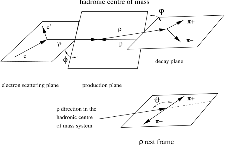
Figure 5: Angle definition for the helicity system in elastic $\rho$ meson production.

Specific relations between the amplitudes, leading to predictions for the values of several matrix elements, follow from additional hypotheses.

• $s$–channel helicity conservation
  For the case of $s$-channel helicity conservation (SCHC), the helicity of the virtual photon is retained by the $\rho$ meson and the helicity of the proton is unchanged:

  $$T_{\lambda_{\rho}\lambda_{N^{\prime}},\lambda_{\gamma}\lambda_{N}}=T_{\lambda_{\rho}\lambda_{N^{\prime}},\lambda_{\gamma}\lambda_{N}}\ \delta_{\lambda_{\rho}\lambda_{\gamma}}\ \delta_{\lambda_{N^{\prime}}\lambda_{N}}\ .$$ (26)

  Single and double helicity flip amplitudes then vanish so that (omitting the nucleon helicities):

  $$T_{\lambda_{\rho}\lambda_{\gamma}}=T_{01}=T_{10}=T_{0-1}=T_{-10}=0,$$ (27)

  $$T_{-11}=T_{1-1}=0,$$ (28)

  and all matrix elements become zero, except five:

  $$\mbox{$r_{00}^{04}$},\ \ \ \mbox{$r_{1-1}^{1}$},\ \ \ {\rm Im}\ \mbox{$r_{1-1}^{2}$},\ \ \ {\rm Re}\ \mbox{$r_{10}^{5}$},\ \ \ {\rm Im}\ \mbox{$r_{10}^{6}$}\ .$$ (29)

  Furthermore, the following relationships occur between these elements:

  $$\ \ \ \mbox{$r_{1-1}^{1}$}\ =\ -\ {\rm Im}\ \mbox{$r_{1-1}^{2}$},\ \ \ {\rm Re}\ \mbox{$r_{10}^{5}$}\ =\ -\ {\rm Im}\ \mbox{$r_{10}^{6}$}\ .$$ (30)

• Natural parity exchange
  Natural parity exchange (NPE) is defined by the following relations between the amplitudes:

  $$T_{-\lambda_{\rho}\lambda_{N^{\prime}},-\lambda_{\gamma}\lambda_{N}}=(-1)^{\lambda_{\rho}-\lambda_{\gamma}}\ T_{\lambda_{\rho}\lambda_{N^{\prime}},\lambda_{\gamma}\lambda_{N}}\ .$$ (31)

In Table 2, the expressions of the matrix elements are given in terms of the helicity amplitudes for two specific sets of assumptions. In column 2, the double helicity flip amplitudes $T_{1-1}$ and $T_{-11}$ and the single flip amplitudes $T_{10}$ and $T_{-10}$ for the production of transversely polarised $\rho$ mesons by longitudinal photons are neglected, and the NPE relations $T_{0-1}=-T_{01}$ and $T_{-1-1}=T_{11}$ are assumed (see the discussion in section 5.3 and the presentation of the QCD model [31], in particular eq. (45), in section 5.4.4). In column 3, the matrix elements are given for the case of SCHC (i.e. neglecting all helicity flip amplitudes) and assuming the NPE relation $T_{-1-1}=T_{11}$. The nucleon helicities $\lambda_{N}$ and $\lambda_{N^{\prime}}$ are omitted from the amplitudes, $T$, for brevity.

The matrix elements can be measured as the projections of the decay angular distribution (eq. 24) onto orthogonal trigonometric functions of the angles $\theta$, $\varphi$ and $\phi$, which are listed in Appendix C of ref. [30]. The average values of these functions, for the 1996 data and for the kinematic domain defined in Table 1, provide the measurements presented in Table 3. The results are also presented in Figs. 6$-$8 (and in Tables 4$-$6) as a function of $Q^{2}$, $W$ and $t$. Statistical and systematic errors are given separately, the systematic errors being computed here, and in the rest of section 5, as described in section 3.1. The data sample is not corrected for the small backgrounds due to proton dissociation, $\omega$ and $\phi$ production and radiative effects.

Within the measurement precision, the matrix elements presented in Table 3 and in Figs. 6$-$8 generally follow the SCHC predictions (with the NPE relation $T_{-1-1}=T_{11}$). This is not the case, however, for the $r_{00}^{5}$ element, which is significantly different from zero (see also the discussion of the distribution of the angle $\phi$ in section 5.3). It has been checked that this effect is not an artifact of the Monte Carlo simulation used to correct the data for detector acceptance effects [12].

As will be discussed in section 5.3, the violation of SCHC is small. Information on the photon polarisation can thus be obtained from the measurements of the spin density matrix elements using SCHC as a first order approximation. This analysis is performed in section 5.2. The violation of SCHC is then studied in more detail in section 5.3. For these analyses, the good description of the data provided by the function $W$($\cos\theta$, $\varphi$, $\phi$) is verified through various angular distributions. Finally, section 5.4 presents comparisons of the results with model predictions.

Element	NPE and $T_{1-1}$ = $T_{10}$ = 0	NPE and SCHC
$r^{04}_{00}$	$\frac{1}{1+\epsilon R}\ \left(\frac{|T_{01}|^{2}}{|T_{11}|^{2}+|T_{01}|^{2}}+\epsilon R\right)$	$\frac{\epsilon R}{1+\epsilon R}$
${\rm Re}\ r^{04}_{10}$	$\frac{1}{2}\ \frac{1}{1+\epsilon R}\ \frac{1}{|T_{11}|^{2}+|T_{01}|^{2}}\ {\rm Re}\ (T_{11}T^{*}_{01}$)	0
$r^{04}_{1-1}$	0	0
$r^{1}_{00}$	$\frac{-1}{1+\epsilon R}\ \frac{|T_{01}|^{2}}{|T_{11}|^{2}+|T_{01}|^{2}}$	0
$r^{1}_{11}$	0	0
${\rm Re}\ r^{1}_{10}$	$-{\rm Re}\ \mbox{$r_{10}^{04}$}$	0
$r^{1}_{1-1}$	$\frac{1}{2}\ \frac{1}{1+\epsilon R}\ \frac{|T_{11}|^{2}}{|T_{11}|^{2}+|T_{01}|^{2}}$	$\frac{1}{2}\frac{1}{1+\epsilon R}$
${\rm Im}\ r^{2}_{10}$	${\rm Re}\ \mbox{$r_{10}^{04}$}$	0
${\rm Im}\ r^{2}_{1-1}$	$-\mbox{$r_{1-1}^{1}$}$	$-r^{1}_{1-1}$
$r^{5}_{00}$	$\frac{\sqrt{2R}}{1+\epsilon R}\ \frac{1}{|T_{00}|\sqrt{|T_{11}|^{2}+|T_{01}|^{2}}}\ {\rm Re}\ (T_{00}T^{*}_{01})$	0
$r^{5}_{11}$	0	0
${\rm Re}\ r^{5}_{10}$	$\frac{1}{2\sqrt{2}}\ \frac{\sqrt{R}}{1+\epsilon R}\ \frac{1}{|T_{00}|\sqrt{|T_{11}|^{2}+|T_{01}|^{2}}}\ {\rm Re}\ (T_{11}T^{*}_{00})$	$\frac{1}{2\sqrt{2}}\ \frac{\sqrt{R}}{1+\epsilon R}\ \frac{1}{|T_{11}||T_{00}|}{\rm Re}\ (T_{11}T^{*}_{00})$
$r^{5}_{1-1}$	0	0
${\rm Im}\ r^{6}_{10}$	$-{\rm Re}\ \mbox{$r_{10}^{5}$}$	$-{\rm Re}\ r^{5}_{10}$
${\rm Im}\ r^{6}_{1-1}$	0	0

Table 2: Spin density matrix elements for the elastic electroproduction of $\rho$ mesons, expressed as a function of the helicity amplitudes $T_{\lambda_{\rho}\ \lambda_{\gamma}}$: second column: the single-flip $T_{10}$ and double-flip $T_{1-1}$ amplitudes are neglected and the NPE relations (31) are assumed for the other amplitudes; third column: the SCHC conditions and the NPE relation $T_{-1-1}=T_{11}$ are assumed (i.e. the $T_{01}$ helicity flip amplitude is also neglected). $R$ is the ratio of cross sections for $\rho$ production by longitudinal and transverse photons. The nucleon helicities are omitted for brevity.

Element	Measurement
$r^{04}_{00}$	0.674	$\pm$ 0.018	${}^{+0.051}_{-0.036}$
${\rm Re}\ r^{04}_{10}$	0.011	$\pm$ 0.012	${}^{+0.007}_{-0.001}$
$r^{04}_{1-1}$	-0.010	$\pm$ 0.013	${}^{+0.004}_{-0.003}$
$r^{1}_{00}$	-0.058	$\pm$ 0.048	${}^{+0.013}_{-0.011}$
$r^{1}_{11}$	0.002	$\pm$ 0.034	${}^{+0.006}_{-0.006}$
${\rm Re}\ r^{1}_{10}$	-0.018	$\pm$ 0.016	${}^{+0.010}_{-0.014}$
$r^{1}_{1-1}$	0.122	$\pm$ 0.018	${}^{+0.004}_{-0.005}$
${\rm Im}\ r^{2}_{10}$	0.023	$\pm$ 0.016	${}^{+0.010}_{-0.009}$
${\rm Im}\ r^{2}_{1-1}$	-0.119	$\pm$ 0.018	${}^{+0.010}_{-0.005}$
$r^{5}_{00}$	0.093	$\pm$ 0.024	${}^{+0.019}_{-0.010}$
$r^{5}_{11}$	0.008	$\pm$ 0.017	${}^{+0.008}_{-0.012}$
${\rm Re}\ r^{5}_{10}$	0.146	$\pm$ 0.008	${}^{+0.006}_{-0.006}$
$r^{5}_{1-1}$	-0.004	$\pm$ 0.009	${}^{+0.001}_{-0.003}$
${\rm Im}\ r^{6}_{10}$	-0.140	$\pm$ 0.008	${}^{+0.002}_{-0.004}$
${\rm Im}\ r^{6}_{1-1}$	0.002	$\pm$ 0.009	${}^{+0.003}_{-0.000}$

Table 3: Spin density matrix elements for the elastic electroproduction of $\rho$ mesons, measured for the 1996 data sample as the average values of the corresponding orthogonal functions of the $\rho$ meson production and decay angles (see Appendix C of ref. [30]). The first errors are statistical, the second systematic.

Figure 6: Spin density matrix elements for elastic electroproduction of $\rho$ mesons, measured for three values of $Q^{2}$ with the 1996 data sample. The inner error bars are statistical and the full error bars include the systematic errors added in quadrature. The dashed lines indicate the expected null values in the case of SCHC.

Figure 7: Spin density matrix elements for elastic electroproduction of $\rho$ mesons, measured for three values of $W$ with the 1996 data sample. The inner error bars are statistical and the full error bars include the systematic errors added in quadrature. The dashed lines indicate the expected null values in the case of SCHC.

Figure 8: Spin density matrix elements for elastic electroproduction of $\rho$ mesons, measured for three values of $t$ with the 1996 data sample. The inner error bars are statistical and the full error bars include the systematic errors added in quadrature. The dashed lines indicate the expected null values in the case of SCHC.

5.2 Helicity Conserving Amplitudes

5.2.1 Ratio of the Longitudinal and Transverse Cross Sections

After integration over the angles $\varphi$ and $\phi$, the angular distribution (eq. 24) takes the form

$$W(\mbox{$\cos\theta$})\propto 1-\mbox{$r_{00}^{04}$}+(3\ \mbox{$r_{00}^{04}$}-1)\ \cos^{2}\theta\ .$$ (32)

In Fig. 9, the $\cos\theta$ distributions for the 1996 data are presented for six bins in $Q^{2}$, and the results of fits to eq. (32) are superimposed. As can be observed from the figures, the quality of the fits is good. The resulting measurements of $r^{04}_{00}$ are in good agreement with those presented in Figs. 6$-$8 and in Tables 4$-$6.

Figure 9: Acceptance corrected $\cos\theta$ distributions for the 1996 data sample in six bins in $Q^{2}$. The curves are the result of fits to the form of eq. (32). The errors on the data points are statistical only.

In the case of SCHC, the matrix element $r_{00}^{04}$ provides a direct measurement of $R$, the ratio of cross sections for $\rho$ production by longitudinal and transverse virtual photons (see Table 2, column 3):

$$\mbox{$R$}=\frac{\sigma_{L}}{\sigma_{T}}=\frac{1}{\varepsilon}\ \frac{\mbox{$r_{00}^{04}$}}{1-\mbox{$r_{00}^{04}$}}\ .$$ (33)

As the SCHC violating amplitudes are small compared to the helicity conserving ones (see section 5.3), eq. (33) can be used assuming SCHC to estimate $R$.

Figure 10: The ratio $R$ of cross sections for elastic $\rho$ meson electroproduction by longitudinal and transverse photons, measured in the SCHC approximation and presented as a function of $Q^{2}$. For the present measurements (full circles), the inner error bars are statistical and the full error bars include the systematic errors added in quadrature. The other measurements are from H1 [26] and ZEUS [28] in photoproduction, and from CHIO [3], NMC [4], E665 [5], H1 [1] and ZEUS [2] in electroproduction.

The values of $R$ deduced from eq. (33) using the results of the fits of the $\cos\theta$ distributions to eq. (32) are presented in Fig. 10 (and in Table 7) as a function of $Q^{2}$, together with other measurements performed assuming SCHC [1, 2, 3, 4, 5, 26, 28]. It is observed that $R$ rises steeply at small $Q^{2}$, and that the longitudinal cross section dominates over the transverse cross section for $Q^{2}\mathrel{\hbox to0.0pt{\lower 4.0pt\hbox{\hskip 1.0pt$\sim$}\hss}\raise 1.0pt\hbox{$>$}}$ 2 ${\rm GeV}^{2}$. However, the rise is non-linear, with a weakening dependence at large $Q^{2}$ values. No significant $W$ dependence of the behaviour of $R$ as a function of $Q^{2}$ is suggested by the comparison of the fixed target and HERA results.

5.2.2 Longitudinal$-$Transverse Interference

In the case of NPE and SCHC, the decay angular distribution $W$($\cos\theta$, $\varphi$, $\phi$) reduces to a function of two variables, $\cos\theta$ and $\psi$, where $\psi=\phi-\mbox{$\varphi$}$ is the angle between the electron scattering plane and the $\rho$ meson decay plane:

$$W(\mbox{$\cos\theta$},\psi)=\frac{3}{8\pi}\ \frac{1}{1+\varepsilon\ R}\ \left\{\ \sin^{2}\theta\ (1+\varepsilon\ \cos 2\psi)\frac{}{}\right.$$

$$+\left.2\ \varepsilon\ R\ \cos^{2}\theta-\sqrt{2\varepsilon\ (1+\varepsilon)\ R}\ \cos\delta\sin 2\theta\cos\psi\right\}\ .$$ (34)

Here $\delta$ is the phase between the transverse $T_{11}$ and the longitudinal $T_{00}$ amplitudes:

$$T_{00}\ T_{11}^{*}=|T_{00}|\ |T_{11}|\ e^{-i\delta}$$ (35)

and

$$\cos\delta=\frac{1+\varepsilon\ R}{\sqrt{R/2}}\left({\rm Re}\ \mbox{$r_{10}^{5}$}-{\rm Im}\ \mbox{$r_{10}^{6}$}\right)\ .$$ (36)

A two-dimensional plot of the $\cos\theta$ and $\psi$ variables is presented in Fig. 11 for the 1996 data. A fit of eq. (34) to these data gives:

$$\cos\delta=0.925\pm 0.022\ ^{+0.011}_{-0.022}\ .$$ (37)

This number is in agreement within errors with the value of $\cos\delta$ computed from eqs. (33) and (36) using the measurements of $r_{00}^{04}$, Re $r_{10}^{5}$ and Im $r_{10}^{6}$ given in Table 3.

Fig. 12 (and Table 8) presents the measurements of $\cos\delta$ as a function of $Q^{2}$, $W$ and $t$. No significant evidence is found for a variation in the phase between the transverse and longitudinal amplitudes with these variables. That these amplitudes are nearly in phase was already observed at lower energy [3, 6, 32].

Figure 11: Acceptance corrected plot of the event distribution in $\cos\theta$ and $\psi$ for the 1996 data sample.

Figure 12: Measurements of the $\cos\delta$ parameter as a function of $Q^{2}$, $W$ and $t$, obtained assuming SCHC and NPE from fits to the ($\cos\theta$, $\psi$) distributions. The inner error bars are statistical and the full error bars include the systematic errors added in quadrature.

5.2.3 The $\psi$ Distribution

Fig. 13 shows the distributions of the angle $\psi$ for five bins in $Q^{2}$. They are well described by the function

$$W(\psi)=\frac{1}{2\pi}\ (1+2\ \varepsilon\ \mbox{$r_{1-1}^{1}$}\ \cos 2\psi)\ ,$$ (38)

obtained from the integration over $\cos\theta$ of the function $W$($\cos\theta$, $\varphi$, $\phi$) (eq. 24), assuming SCHC. Measurements of the $r^{1}_{1-1}$ matrix element extracted from fits to eq. (38) as a function of $Q^{2}$, $W$ and $t$ are in good agreement with the measurements presented in Figs. 6$-$8 and in Tables 4$-$6, which supports the fact that SCHC is a good approximation for the present data.

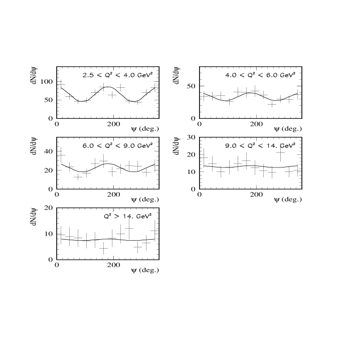
Figure 13: Acceptance corrected distributions of the $\psi$ angle for the 1996 data sample in five bins in $Q^{2}$. The curves are the result of fits to the form of eq. (38). The errors on the data points are statistical only.

5.3 Helicity Flip Amplitudes

Distributions of the angle $\phi$ are presented in Fig. 14 for six bins in $Q^{2}$. These distributions, as well as the corresponding distributions for bins in $W$ and $t$, exhibit significant variation in $\cos\phi$. Variation in $\cos 2\phi$ is compatible with zero. They are well described by the function

$$W(\phi)\propto 1-\varepsilon\ \cos 2\phi\ (2\ \mbox{$r_{11}^{1}$}+\mbox{$r_{00}^{1}$})+\sqrt{2\varepsilon(1+\varepsilon)}\cos\phi\ (2\ \mbox{$r_{11}^{5}$}+\mbox{$r_{00}^{5}$})\ ,$$ (39)

obtained from the integration of the decay angular distribution (eq. 24) over $\cos\theta$ and $\varphi$.

The combinations of the matrix elements $(2\ \mbox{$r_{11}^{1}$}+\mbox{$r_{00}^{1}$})$ and $(2\ \mbox{$r_{11}^{5}$}+\mbox{$r_{00}^{5}$})$, extracted as a function of $Q^{2}$, $W$ and $t$, are presented in Fig. 15 (and in Table 9). There is no indication for a significant deviation from zero of the combination $(2\ \mbox{$r_{11}^{1}$}+\mbox{$r_{00}^{1}$})$, which is consistent with the measurements presented in Figs. 6$-$8 and in Tables 4$-$6. In contrast, the combination $(2\ \mbox{$r_{11}^{5}$}+\mbox{$r_{00}^{5}$})$ is significantly different from zero. As discussed in section 5.1, this effect is attributed to a violation of SCHC for the matrix element $r_{00}^{5}$.

As can be deduced from the second column of Table 2, the $r_{00}^{5}$ matrix element is approximately proportional to the amplitude $T_{01}$ for a transverse photon to produce a longitudinal $\rho$ meson:

$$r^{5}_{00}\simeq\frac{\sqrt{2R}}{1+\varepsilon R}\frac{|T_{01}|}{|T_{11}|}\ ,$$ (40)

where the term $|T_{01}|^{2}$ has been neglected with respect to $|T_{11}|^{2}$ in the denominator and the amplitudes $T_{00}$ and $T_{01}$ are assumed to be in phase and purely imaginary [31].

With these approximations and with $\varepsilon\simeq\ 1$, the measurement of $r_{00}^{5}$ allows the determination of the ratio of the $T_{01}$ amplitude to the non-flip amplitudes $\sqrt{|T_{00}|^{2}+|T_{11}|^{2}}$ for the present $Q^{2}$ domain:

$$\frac{|T_{01}|}{\sqrt{|T_{00}|^{2}+|T_{11}|^{2}}}\simeq\frac{|T_{01}|}{|T_{11}|\sqrt{1+R}} \simeq \ r^{5}_{00}\ \sqrt{\frac{1+R}{2R}}$$ (41)

$$\simeq 8\pm 3\%\ ,$$ (42)

using the results in Table 3 and eq. (33). This value is of the order of magnitude, or slightly lower than those found, with large errors, at lower energy and for $\langle Q^{2}\rangle\simeq 0.5$ ${\rm GeV}^{2}$ ($15-20\%$ for $W\simeq$ 2.5 GeV [6] and $11-14\%$ for $10<W<16$ GeV [3]).

The other helicity flip amplitudes are consistent with zero within the present measurement precision, as can be deduced from the fact that among the matrix elements which vanish under SCHC only the $r_{00}^{5}$ element is measured to be non-zero. This is confirmed by the study of the $\varphi$ distribution. After integration over $\cos\theta$ and $\phi$, the decay distribution (24) reduces to

$$W(\mbox{$\varphi$})\propto 1-2\ \mbox{$r_{1-1}^{04}$}\cos 2\mbox{$\varphi$}\ .$$ (43)

Figure 14: Acceptance corrected distributions of the $\phi$ angle for the 1996 data sample in six bins in $Q^{2}$. The curves are the result of fits to the form of eq. (39). The errors on the data points are statistical only.

Figure 15: Measurements of the combinations of matrix elements $2\mbox{$r_{11}^{1}$}+\mbox{$r_{00}^{1}$}$ and $2\mbox{$r_{11}^{5}$}+\mbox{$r_{00}^{5}$}$, as a function of $Q^{2}$, $W$ and $t$, obtained from fits to the $\phi$ distributions. The inner error bars are statistical and the full error bars include the systematic errors added in quadrature. The dashed lines indicate the null values which are expected in the case of SCHC.

This distribution is compatible with being constant for all bins in $Q^{2}$, $W$ and $t$, supporting the observation that the matrix element $r_{1-1}^{04}$ is consistent with zero. The expression for this matrix element contains a term proportional to $T_{11}T^{*}_{1-1}$, the interference between the helicity conserving transverse amplitude and the double-flip amplitude, and a term proportional to the square of the single flip contribution $T^{2}_{10}$ (NPE is assumed). The constant $\varphi$ distributions thus indicate that the helicity amplitudes $T_{1-1}$ and $T_{10}$ are compatible with zero.

Another way to study the amplitude $T_{10}$ is to compare the measured values of the $r_{1-1}^{1}$ and $r_{00}^{04}$ matrix elements, which are related by

$$\mbox{$r_{1-1}^{1}$}~{}=\frac{1}{2}~{}(1-\mbox{$r_{00}^{04}$})\$$ (44)

if, and only if, $T_{10}=0$ (NPE is assumed). Relation (44) is satisfied within errors for the measurements presented in Figs. 6$-$8 and in Tables 4$-$6.

5.4 Comparison with Models

Numerous models for the electroproduction of vector mesons based on VDM or QCD have been proposed. Most of them predict, for the present $Q^{2}$ domain, a linear increase with $Q^{2}$ of the ratio $R$ of the longitudinal to transverse cross sections, in disagreement with the results presented in Fig. 10.

However, several recent models predict a slower increase of $R$ at high $Q^{2}$ [31, 33, 34, 35], which corresponds better to the trend in the data. One of them offers in addition full predictions for the spin density matrix elements [31]. In the rest of this section, we concentrate on the comparison of these model predictions with the present measurements.

5.4.1 Generalised Vector Dominance

A calculation based on the Generalised Vector Dominance Model (GVDM) has been performed by Schildknecht, Schuler and Surrow [33]. It takes into account a continuous mass spectrum of vector meson states, with destructive interferences between neighbouring states. This leads to a non-linear $Q^{2}$ dependence for the ratio $R$, in contrast with the conventional VDM predictions. The ratio $R$ tends asymptotically to a constant value, defined by effective transverse and longitudinal masses which must be obtained from a fit to experimental data. The domain of applicability of the model extends in $Q^{2}$ down to photoproduction.

In Fig. 16, the prediction of this model is compared to the measurement of $R$ as a function of $Q^{2}$, using the best set of parameters (“2-par. fit” in [33]). The data are the HERA measurements presented in Fig. 10.

Figure 16: The ratio $R$ of the longitudinal to transverse photon cross sections for elastic $\rho$ meson electroproduction as a function of $Q^{2}$. The data are the HERA measurements as in Fig. 10. The curves are the predictions of the models of Royen and Cudell [35] (solid), of Martin, Ryskin and Teubner (dashed) [34] and of Schildknecht, Schuler and Surrow [33] (dotted), for the HERA energy range.

5.4.2 Parton–Hadron Duality

Martin, Ryskin and Teubner have observed that QCD calculations of the $\rho$ cross section that convolute the scattering amplitude with the $\rho$ wave function give transverse cross sections which fall off too quickly with increasing $Q^{2}$ and thus lead to values of $R$ which are too large at high $Q^{2}$ [34]. They have proposed an alternative approach, in which open $q\bar{q}$ production is considered in a broad mass interval containing the $\rho$ meson. Hadronisation proceeds predominantly into two pion states, following phase space considerations. The hard interaction is modelled through two gluon exchange (or a gluon ladder), which induces a dependence on the parameterisation of the gluon density in the proton. The main uncertainties of the model come from the higher order corrections and from the choice of the mass interval embracing the $\rho$ meson. However, the prediction for the ratio $R$ of the cross sections has little sensitivity to these uncertainties.

Fig. 16 presents the prediction of the model of Martin, Ryskin and Teubner, computed with the MRS(R4) parameterisation [36, 37] for the gluon content of the proton.

5.4.3 Quark Off-Shellness Model

Another model based on lowest-order perturbative QCD calculations has been proposed by Royen and Cudell [35]. The $\rho$ meson production is computed from the $q\overline{q}$ Fock state of the photon, convoluted with the amplitude for hard scattering modelled as two-gluon exchange. A proton form factor and a meson vertex wave function, including Fermi motion, are part of the calculation. The specific feature of the model is that the constituent quarks are allowed to go off-shell. The $W$ dependence of the cross section is not predicted, but the $Q^{2}$ and $t$ dependences are. The uncertainties of the model come from the choice of the constituent quark mass $m_{q}$ and the Fermi momentum $p_{F}$.

The prediction of the model of Royen and Cudell is shown in Fig. 16 for $m_{q}$ = 0.3 GeV and $p_{F}$ = 0.3 GeV. When $m_{q}$ and $p_{F}$ are varied by $\pm$ 50 MeV, the $R$ value changes by about 15% and 30%, respectively, for $Q^{2}$ = 10 ${\rm GeV}^{2}$.

5.4.4 Predictions of Polarisation

Ivanov and Kirschner have provided predictions for the full set of 15 elements of the spin density matrix, based on perturbative QCD [31]. This model predicts a violation of SCHC at high $Q^{2}$, the largest helicity-flip amplitude being $T_{01}$, with:

$$|T_{00}|>|T_{11}|>|T_{01}|>|T_{10}|>|T_{1-1}|$$ (45)

for the HERA kinematical domain. The ratios $|T_{11}|/|T_{00}|$, $|T_{01}|/|T_{00}|$ and $|T_{10}|/|T_{00}|$ depend on $t$, $Q^{2}$, $M$ and $\gamma$, where $M$ is the invariant mass of the $q\overline{q}$ pair and $\gamma$ is the anomalous dimension of the gluon density ($xg(x,\mbox{$Q^{2}$})\propto Q^{2\gamma}$). The ratio $|T_{1-1}|/|T_{00}|$ depends also on the gluon density at the scale $Q^{2}/4$.

Figure 17: Spin density matrix elements for elastic electroproduction of $\rho$ mesons, for three values of $Q^{2}$. The data are the same as in Fig. 6. The curves are the predictions of the model of Ivanov and Kirschner [31] for the GRV 94HO parameterisation of the gluon density in the proton.

Fig. 17 shows the predicted values of the matrix elements obtained with the parameterisation GRV 94HO of the gluon density in the proton [36, 38], compared to the measurements presented in Fig. 6. This density is assumed to be valid throughout the range of $Q^{2}$ of the data. For higher $Q^{2}$ values, other parameterisations give predictions differing by much less than the measurement uncertainties. Reasonable agreement of the model predictions with the data is observed, with a correct prediction of the hierarchy between the amplitudes which are measured to be non-zero, and of the magnitude of the matrix element $r_{00}^{5}$.

6 Cross Sections

6.1 $t$ Dependence of the $ep$ Cross Section

The acceptance corrected $t$ distributions of the selected events with $\mbox{$|t|$}<0.5~{}\mbox{${\rm GeV}^{2}$}$ are presented in Fig. 18 for five bins in $Q^{2}$. To study the $t$ dependence of elastic $\rho$ production, these distributions are fitted as the sum of three exponentials corresponding to the elastic component, the diffractive component with proton dissociation and the non-resonant two-pion background. The elastic component is fitted with a free slope parameter $b$, whereas the contribution of diffractive $\rho$ events with proton dissociation, which amounts to $11\pm 5\%$ of the elastic signal, has a fixed slope parameter $b_{pd}=2.5\pm 1.0~{}\mbox{${\rm GeV}^{-2}$}$ (see section 3.2.2). The non-resonant background, amounting to $1\pm 1\%$ of the signal, also has a fixed slope parameter, $b_{nr}$ = 0.3 $\pm$ 0.1 ${\rm GeV}^{-2}$, extracted from the present data at large $|t|$ values.

Figure 18: Acceptance corrected $t$ distributions for the 1996 data sample, for five bins in $Q^{2}$. The full curves correspond to a fit of the distributions as the sum of three exponentials, corresponding to the elastic signal (dashed curves), 11% background of proton dissociation events with slope $b_{pd}$ = 2.5 ${\rm GeV}^{-2}$ (dotted), and 1% non-resonant background with slope $b_{nr}$ = 0.3 GeV^-2 (not visible on the plots). The errors on the data points are statistical only.

The fitted exponential slope parameters, $b$, for elastic events are presented as a function of $Q^{2}$ in Fig. 19 (and in Table 10), together with H1 [1, 26], ZEUS [2, 28, 39] and fixed target [3, 4, 5] measurements. The systematic errors are computed by varying the parameters of the Monte Carlo simulation used for the acceptance corrections (see section 3.1), by varying the amounts of background contributions and their slopes within the quoted errors, and by varying the binning and the limits of the fits.

The present measurements confirm the decrease of $b$ when $Q^{2}$ increases from photoproduction to the deep-inelastic domain, presumably reflecting the decrease of the transverse size of the virtual photon. It is also observed in Fig. 19 that at low $Q^{2}$ ($Q^{2}$ $\mathrel{\hbox to0.0pt{\lower 4.0pt\hbox{\hskip 1.0pt$\sim$}\hss}\raise 1.0pt\hbox{$<$}}$ 2 ${\rm GeV}^{2}$) measurements at HERA lie systematically above the low energy fixed target results. This may indicate shrinkage of the diffractive peak as $W$ increases. At higher $Q^{2}$, given the experimental errors, no significant information on a possible shrinkage of the $t$ distribution can be extracted within the $W$ range of the present experiment.

Figure 19: Measurement of the slope parameter $b$ of the exponential $t$ dependence for elastic $\rho$ production. For the present measurements (full circles), the inner error bars are statistical and the full error bars include the systematic errors added in quadrature. The other measurements are from H1 [26] and ZEUS [28, 39] in photoproduction, and from CHIO [3], NMC [4], E665 [5], H1 [1] and ZEUS [2] in electroproduction. It should be noted that the definition of the parameter $b$ is not unique (see text).

Figure 20: $Q^{2}$ dependence of the slope parameter $b$ for $\rho$ elastic production by H1 (these and previous measurements [1, 26]), compared to the predictions of the model of Royen and Cudell [35] for the HERA energy range, presented in the form of the variable $1/\langle\mbox{$|t|$}\rangle$.

The $Q^{2}$ evolution of the $t$ distribution in the model of Royen and Cudell [35] is compared in Fig. 20 to the present measurements, in the form of the variable $1/\langle\mbox{$|t|$}\rangle$, which coincides with $b$ for an exponential distribution. The trend of the data is reproduced.

6.2 $Q^{2}$ Dependence of the $\gamma^{*}p$ Cross Section

The $\gamma^{*}p$ cross section for $\rho$ elastic production is extracted from the $ep$ cross section using the relation:

$$\frac{{\rm d}^{2}\sigma(ep\rightarrow e\rho p)}{{\rm d}y\ {\rm d}\mbox{$Q^{2}$}}=\Gamma\ \sigma(\gamma^{*}p\rightarrow\rho p)=\Gamma\ \sigma_{T}(\gamma^{*}p\rightarrow\rho p)\ (1+\varepsilon R)\ ,$$ (46)

where $\Gamma$ is the flux of virtual photons [40], given by:

$$\Gamma=\frac{\alpha\ (1-y+y^{2}/2)}{\pi\ y\ \mbox{$Q^{2}$}}\ ,$$ (47)

$\alpha$ being the fine structure constant. The flux is integrated over each kinematic domain using the measured $Q^{2}$ and $W$ dependences of the $\gamma^{*}p$ cross section.

Figure 21: Cross section measurements for the process $\gamma^{*}p\rightarrow\rho p$ plotted as a function of $Q^{2}$ for $W=75~{}\mbox{\rm GeV}$ (the ZEUS measurements [2] have been scaled to $W=75~{}\mbox{\rm GeV}$. The inner error bars are statistical and the full error bars include the systematic errors added in quadrature. The curve corresponds to a fit to the present data of the form of eq. (49), with $n=2.24$.

The $\gamma^{*}p$ cross section is presented in Fig. 21 (and in Table 11) as a function of $Q^{2}$, for a common value $W=75~{}\mbox{\rm GeV}$. It is obtained from the fits described in section 4, which take into account the $Q^{2}$ dependent skewing of the $m_{\pi\pi}$ mass distribution. The cross section is quoted for a relativistic Breit-Wigner distribution of the $\rho$ mass, described by eqs. (19) and (20), for the mass interval

$$2\ m_{\pi}\leq\mbox{$m_{\pi\pi}$}\leq\mbox{$m_{\rho}$}\ +5\ \mbox{$\Gamma_{\rho}$}\ .$$ (48)

The use of two alternative forms to eq. (20) in parameterising the width $\Gamma(\mbox{$m_{\pi\pi}$})$ [24] would cause an increase of the cross section by 5%, which is included in the systematic errors. The background contributions of $\rho$ diffractive production with proton dissociation, of $\omega$ and $\phi$ elastic production, and the non-resonant background are subtracted assuming the same distribution in $Q^{2}$ as for the signal. The uncertainties in these backgrounds are included in the systematic errors. The $Q^{2}$ dependent losses induced by the $\mbox{$|t|$}<0.5~{}\mbox{${\rm GeV}^{2}$}$ cut are corrected for on a bin-by-bin basis, according to the measured $b$ slope parameters (see section 6.1). The data are corrected for the losses of events due to noise in the detectors FMD and PRT (5 $\pm$ 3%) and LAr (10 $\pm$ 3%). Acceptance and efficiency effects and their errors are determined as described in section 3.1. The errors on the extrapolations of the cross sections to the common value $W=75~{}\mbox{\rm GeV}$ and to the quoted $Q^{2}$ values are estimated by varying the assumed $W$ and $Q^{2}$ dependences of the cross section according to the limits of the present measurements. The radiative corrections are very small for the chosen value of the $E-p_{z}$ cut and for the procedure used to compute the kinematic variables (see section 2.2); an error of 4% accounts for the relevant uncertainties in the $Q^{2}$ and $W$ dependences of the cross section, for higher order processes, and for detector effects not simulated in detail. The systematic errors on the cross section measurements also include an uncertainty of 2% in the luminosity, and the uncertainties due to limited Monte Carlo statistics.

A parameterisation of the $Q^{2}$ dependence of the cross section in the form

$$\sigma(\gamma^{*}p)\propto\frac{1}{(\mbox{$Q^{2}$}+m^{2}_{\mbox{$\rho$}})^{n}}$$ (49)

is shown superimposed on Fig. 21. It is obtained by a fit to the present data with the result

$$n=2.24\pm 0.09\ .$$ (50)

The uncertainty on this value is determined using the statistical and the non-correlated systematic errors only. The nominal normalisations are used for the 1995 and 1996 data sets, which agree within one standard deviation. The quality of the fit for the full $Q^{2}$ range $1\leq\mbox{$Q^{2}$}\leq 35~{}\mbox{${\rm GeV}^{2}$}$ is good: $\chi^{2}/{\rm ndf}$ = 13.3 / 20.

Fig. 21 presents in addition the measurements of the ZEUS collaboration [2], scaled to the value W = 75 GeV. Agreement is observed between the results of the two experiments.

Figure 22: Cross section for the process $\gamma^{*}p\rightarrow\rho p$, plotted as a function of $Q^{2}$ for $W=75~{}\mbox{\rm GeV}$ (the data are the same as in Fig. 21). Photoproduction measurements by H1 [26] and ZEUS [28] are also shown. The curves are the predictions of the models of Royen and Cudell [35] (solid), of Martin, Ryskin and Teubner [34] (dashed) and of Schildknecht, Schuler and Surrow [33] (dotted).

In Fig. 22, the $Q^{2}$ dependence of the $\gamma^{*}p$ cross section, including photoproduction measurements [26, 28], is compared with the predictions of the models of Schildknecht, Schuler and Surrow [33], of Martin, Ryskin and Teubner [34] and of Royen and Cudell [35]. The latter model describes the data well down to the photoproduction region.

6.3 $W$ Dependence of the $\gamma^{*}p$ Cross Section

The $\gamma^{*}p$ cross section for $\rho$ elastic production is presented as a function of $W$ for six values of $Q^{2}$ in Fig. 23 (and in Table 12). The extrapolations of the measured cross sections to the chosen $Q^{2}$  values are performed using the $Q^{2}$ dependence given by eqs. (49) and (50). Corrections and systematic errors are determined as described in section 6.2.

To quantify the $W$ dependence of the cross section, a fit is performed for each $Q^{2}$ bin to a power law:

$$\sigma(\gamma^{*}p)\propto W^{\delta}\ ,$$ (51)

as shown in Fig. 23. Only the statistical and the non-correlated systematic errors are used in the fits, and the values of $\chi^{2}/{\rm ndf}$ are reasonable for all $Q^{2}$ bins.

In a Regge context, the parameter $\delta$ can be related to the exchange trajectory:

$$\delta\simeq 4\ [\alpha(\langle t\rangle)-1]\ .$$ (52)

The trajectory is assumed to take a linear form:

$$\alpha(t) = \alpha(0)+\alpha^{\prime}\ t\ .$$ (53)

To extract the effective trajectory intercept $\alpha(0)$, $\langle\mbox{$|t|$}\rangle$ = 1/$b$ is taken from the measured values (see section 6.1). In the absence of a measurement of the $Q^{2}$ dependence of the shrinkage of the $t$ distribution with increasing $W$, the value $\alpha^{\prime}=0.25~{}\mbox{${\rm GeV}^{-2}$}$ is assumed, as measured in hadron$-$hadron interactions [41]. The values obtained for the intercept $\alpha(0)$ as a function of $Q^{2}$ are shown in Fig. 24 (and in Table 13). The inner error bars come from the statistical and non-correlated systematic uncertainties on the cross section measurements. The sensitivity to the choice of $\alpha^{\prime}$ is shown by the outer bars, which contain the variation due to the assumption $\alpha^{\prime}=0$ (i.e. no shrinkage) added in quadrature. The measurements are compared to the values $1.08-1.10$ obtained from fits to the total and elastic hadron–hadron cross sections [41, 42]. They suggest that the intercept of the effective trajectory governing high $Q^{2}$ $\rho$ electroproduction is larger than that describing elastic and total hadronic cross sections.

Figure 23: Cross section for the process $\gamma^{*}p\rightarrow\rho p$ as a function of $W$ for several values of $Q^{2}$. The inner error bars are statistical and the full error bars include the systematic errors added in quadrature. The lines correspond to a fit of the form of eq. (51).

Figure 24: $Q^{2}$ dependence of the intercept $\alpha(0)$ (see eqs. 51 $-$ 53). The inner error bars represent the statistical and non-correlated systematic uncertainties on the cross section measurements, the outer error bars include the variation of the intercept $\alpha(0)$ when assuming $\alpha^{\prime}=0$, added in quadrature. The dashed lines represent the range of values obtained for the “soft pomeron” intercept, as derived from fits to total and elastic hadron$-$hadron cross section measurements [41, 42].

It should be noted that several studies (see e.g. [43]) indicate that QCD based predictions for the $W$ dependence of the $\gamma^{*}p$ cross section are affected by large uncertainties. These are related particularly to the assumptions made concerning the appropriate factorisation scale and the $\rho$ wave function, and also to the choice of the parameterisation of the gluon distribution in the proton.

7 Summary and Conclusions

The elastic electroproduction of $\rho$ mesons has been studied at HERA with the H1 detector, for $1~{}<Q^{2}<60$ GeV² and 30 $<$ $W$ $<$ 140 GeV.

The shape of the ($\pi\pi$) mass distribution has been studied as a function of $Q^{2}$. It indicates significant skewing at low $Q^{2}$, which gets smaller with increasing $Q^{2}$.

The full set of 15 elements of the $\rho$ spin density matrix has been measured as a function of $Q^{2}$, $W$ and $t$, using the decay angular distributions defined in the helicity frame. Except for a small but significant deviation from zero of the $r_{00}^{5}$ element, $s$-channel helicity conservation is found to be a good approximation. For $Q^{2}$ $\mathrel{\hbox to0.0pt{\lower 4.0pt\hbox{\hskip 1.0pt$\sim$}\hss}\raise 1.0pt\hbox{$>$}}$ 2 ${\rm GeV}^{2}$, the longitudinal $\gamma^{*}p$ cross section becomes larger than the transverse cross section, and the ratio $R$ reaches the value $R$ $\simeq$ 3 for $Q^{2}$ $\simeq$ 20 ${\rm GeV}^{2}$. The phase $\delta$ between the longitudinal and transverse amplitudes is measured to be $\cos\delta$ = 0.93 $\pm$ 0.03, assuming natural parity exchange and $s$-channel helicity conservation. The dominant helicity flip amplitude $T_{\lambda_{\rho}=0,\lambda_{\gamma}=1}$ is found to be $8\pm 3\%$ of the non-flip amplitudes. A model based on GVDM [33] and models based on perturbative QCD [34, 35] reproduce the flattening of the ratio $R$ observed at high $Q^{2}$. A QCD based prediction [31] is in qualitative agreement with the measurement of the 15 matrix elements, in that it reproduces the observed hierarchy between the amplitudes which are measured to be non-zero and the magnitude of the matrix element $r_{00}^{5}$.

The $t$ distribution for $\rho$ electroproduction has been studied and the exponential slope parameter $b$ is found to decrease when $Q^{2}$ increases from photoproduction to the deep-inelastic domain.

The $\gamma^{*}p\rightarrow\rho p$ cross section has been measured over the domain 1 $<$ $Q^{2}$ $<$ 35 GeV² and follows a $Q^{2}$ dependence of the form $1/(\mbox{$Q^{2}$}\ +m_{\rho}^{2})^{n}$, with $n$ = 2.24 $\pm$ 0.09. This dependence is well described by a model based on QCD [35].

The $W$ dependence of the $\gamma^{*}p\rightarrow\rho p$ cross section has been measured for six values of $Q^{2}$. The measurements suggest that the intercept of the effective trajectory governing high $Q^{2}$ $\rho$ electroproduction is larger than that describing elastic and total hadronic cross sections.

	Element	2.5 $<$ $Q^{2}$ $<$ 3.5 ${\rm GeV}^{2}$	3.5 $<$ $Q^{2}$ $<$ 6.0 ${\rm GeV}^{2}$	6.0 $<$ $Q^{2}$ $<$ 60 ${\rm GeV}^{2}$
1	$r_{00}^{04}$	0.639 $\pm$ 0.031 ${}^{+0.013}_{-0.010}$	0.695 $\pm$ 0.031 ${}^{+0.019}_{-0.018}$	0.748 $\pm$ 0.033 ${}^{+0.037}_{-0.011}$
2	Re $r_{10}^{04}$	0.018 $\pm$ 0.020 ${}^{+0.004}_{-0.004}$	-0.019 $\pm$ 0.020 ${}^{+0.009}_{-0.003}$	0.036 $\pm$ 0.022 ${}^{+0.006}_{-0.012}$
3	$r_{1-1}^{04}$	-0.020 $\pm$ 0.023 ${}^{+0.002}_{-0.003}$	-0.020 $\pm$ 0.022 ${}^{+0.008}_{-0.001}$	0.016 $\pm$ 0.023 ${}^{+0.003}_{-0.012}$
4	$r_{00}^{1}$	-0.011 $\pm$ 0.081 ${}^{+0.013}_{-0.022}$	-0.085 $\pm$ 0.082 ${}^{+0.021}_{-0.013}$	-0.078 $\pm$ 0.092 ${}^{+0.024}_{-0.002}$
5	$r_{11}^{1}$	-0.019 $\pm$ 0.057 ${}^{+0.016}_{-0.003}$	0.021 $\pm$ 0.057 ${}^{+0.001}_{-0.006}$	0.010 $\pm$ 0.063 ${}^{+0.001}_{-0.009}$
6	Re $r_{10}^{1}$	0.003 $\pm$ 0.028 ${}^{+0.016}_{-0.003}$	-0.022 $\pm$ 0.028 ${}^{+0.015}_{-0.016}$	-0.042 $\pm$ 0.030 ${}^{+0.005}_{-0.007}$
7	$r_{1-1}^{1}$	0.147 $\pm$ 0.032 ${}^{+0.013}_{-0.007}$	0.103 $\pm$ 0.031 ${}^{+0.003}_{-0.005}$	0.081 $\pm$ 0.031 ${}^{+0.010}_{-0.013}$
8	Im $r_{10}^{2}$	0.006 $\pm$ 0.028 ${}^{+0.008}_{-0.004}$	0.049 $\pm$ 0.028 ${}^{+0.015}_{-0.015}$	0.007 $\pm$ 0.030 ${}^{+0.005}_{-0.011}$
9	Im $r_{1-1}^{2}$	-0.156 $\pm$ 0.032 ${}^{+0.014}_{-0.010}$	-0.098 $\pm$ 0.031 ${}^{+0.018}_{-0.007}$	-0.067 $\pm$ 0.032 ${}^{+0.007}_{-0.025}$
10	$r_{00}^{5}$	0.099 $\pm$ 0.040 ${}^{+0.016}_{-0.002}$	0.081 $\pm$ 0.041 ${}^{+0.009}_{-0.013}$	0.107 $\pm$ 0.047 ${}^{+0.015}_{-0.004}$
11	$r_{11}^{5}$	0.002 $\pm$ 0.029 ${}^{+0.002}_{-0.007}$	0.005 $\pm$ 0.029 ${}^{+0.006}_{-0.006}$	0.014 $\pm$ 0.032 ${}^{+0.006}_{-0.012}$
12	Re $r_{10}^{5}$	0.149 $\pm$ 0.013 ${}^{+0.002}_{-0.002}$	0.142 $\pm$ 0.013 ${}^{+0.003}_{-0.002}$	0.133 $\pm$ 0.014 ${}^{+0.003}_{-0.004}$
13	$r_{1-1}^{5}$	-0.019 $\pm$ 0.016 ${}^{+0.005}_{-0.001}$	0.004 $\pm$ 0.016 ${}^{+0.006}_{-0.006}$	0.003 $\pm$ 0.016 ${}^{+0.004}_{-0.010}$
14	Im $r_{10}^{6}$	-0.124 $\pm$ 0.013 ${}^{+0.001}_{-0.001}$	-0.146 $\pm$ 0.013 ${}^{+0.004}_{-0.005}$	-0.146 $\pm$ 0.014 ${}^{+0.004}_{-0.002}$
15	Im $r_{1-1}^{6}$	0.022 $\pm$ 0.016 ${}^{+0.001}_{-0.002}$	-0.014 $\pm$ 0.016 ${}^{+0.003}_{-0.004}$	-0.001 $\pm$ 0.016 ${}^{+0.006}_{-0.003}$

Table 4: Spin density matrix elements for elastic electroproduction of $\rho$ mesons, measured for three values of $Q^{2}$ with the 1996 data sample. The first errors are statistical, the second systematic.

	Element	40 $<$ $W$ $<$ 60 GeV	60 $<$ $W$ $<$ 80 GeV	80 $<$ $W$ $<$ 100 GeV
1	$r_{00}^{04}$	0.671 $\pm$ 0.031 ${}^{+0.031}_{-0.025}$	0.719 $\pm$ 0.031 ${}^{+0.051}_{-0.033}$	0.687 $\pm$ 0.033 ${}^{+0.031}_{-0.016}$
2	Re $r_{10}^{04}$	-0.011 $\pm$ 0.020 ${}^{+0.010}_{-0.007}$	0.025 $\pm$ 0.020 ${}^{+0.011}_{-0.009}$	0.052 $\pm$ 0.021 ${}^{+0.006}_{-0.003}$
3	$r_{1-1}^{04}$	-0.021 $\pm$ 0.023 ${}^{+0.005}_{-0.006}$	0.000 $\pm$ 0.023 ${}^{+0.011}_{-0.010}$	-0.028 $\pm$ 0.024 ${}^{+0.010}_{-0.004}$
4	$r_{00}^{1}$	-0.048 $\pm$ 0.081 ${}^{+0.021}_{-0.019}$	-0.151 $\pm$ 0.082 ${}^{+0.020}_{-0.010}$	0.043 $\pm$ 0.089 ${}^{+0.029}_{-0.026}$
5	$r_{11}^{1}$	-0.013 $\pm$ 0.057 ${}^{+0.008}_{-0.009}$	0.080 $\pm$ 0.057 ${}^{+0.003}_{-0.006}$	-0.060 $\pm$ 0.062 ${}^{+0.021}_{-0.024}$
6	Re $r_{10}^{1}$	-0.002 $\pm$ 0.028 ${}^{+0.006}_{-0.006}$	-0.018 $\pm$ 0.028 ${}^{+0.013}_{-0.022}$	-0.023 $\pm$ 0.030 ${}^{+0.022}_{-0.027}$
7	$r_{1-1}^{1}$	0.225 $\pm$ 0.031 ${}^{+0.002}_{-0.005}$	0.113 $\pm$ 0.031 ${}^{+0.007}_{-0.010}$	0.083 $\pm$ 0.033 ${}^{+0.052}_{-0.044}$
8	Im $r_{10}^{2}$	-0.030 $\pm$ 0.028 ${}^{+0.012}_{-0.008}$	0.105 $\pm$ 0.028 ${}^{+0.006}_{-0.008}$	0.032 $\pm$ 0.030 ${}^{+0.009}_{-0.006}$
9	Im $r_{1-1}^{2}$	-0.132 $\pm$ 0.032 ${}^{+0.016}_{-0.010}$	-0.151 $\pm$ 0.031 ${}^{+0.013}_{-0.009}$	-0.068 $\pm$ 0.033 ${}^{+0.020}_{-0.024}$
10	$r_{00}^{5}$	0.030 $\pm$ 0.041 ${}^{+0.003}_{-0.003}$	0.192 $\pm$ 0.041 ${}^{+0.033}_{-0.013}$	0.114 $\pm$ 0.045 ${}^{+0.007}_{-0.002}$
11	$r_{11}^{5}$	-0.009 $\pm$ 0.029 ${}^{+0.004}_{-0.001}$	-0.015 $\pm$ 0.029 ${}^{+0.004}_{-0.010}$	0.027 $\pm$ 0.031 ${}^{+0.007}_{-0.008}$
12	Re $r_{10}^{5}$	0.177 $\pm$ 0.013 ${}^{+0.015}_{-0.009}$	0.118 $\pm$ 0.013 ${}^{+0.011}_{-0.009}$	0.125 $\pm$ 0.014 ${}^{+0.009}_{-0.009}$
13	$r_{1-1}^{5}$	-0.014 $\pm$ 0.016 ${}^{+0.004}_{-0.008}$	-0.005 $\pm$ 0.016 ${}^{+0.007}_{-0.002}$	-0.018 $\pm$ 0.017 ${}^{+0.007}_{-0.006}$
14	Im $r_{10}^{6}$	-0.148 $\pm$ 0.013 ${}^{+0.003}_{-0.004}$	-0.160 $\pm$ 0.013 ${}^{+0.005}_{-0.006}$	-0.115 $\pm$ 0.014 ${}^{+0.013}_{-0.031}$
15	Im $r_{1-1}^{6}$	-0.005 $\pm$ 0.016 ${}^{+0.002}_{-0.002}$	0.021 $\pm$ 0.016 ${}^{+0.002}_{-0.002}$	-0.014 $\pm$ 0.017 ${}^{+0.009}_{-0.011}$

Table 5: Spin density matrix elements for elastic electroproduction of $\rho$ mesons, measured for three values of $W$ with the 1996 data sample. The first errors are statistical, the second systematic.

	Element	0.0 $<$ $|t|$ $<$ 0.1 ${\rm GeV}^{2}$	0.1 $<$ $|t|$ $<$ 0.2 ${\rm GeV}^{2}$	0.2 $<$ $|t|$ $<$ 0.5 ${\rm GeV}^{2}$
1	$r_{00}^{04}$	0.686 $\pm$ 0.031 ${}^{+0.050}_{-0.039}$	0.706 $\pm$ 0.031 ${}^{+0.059}_{-0.041}$	0.634 $\pm$ 0.033 ${}^{+0.042}_{-0.032}$
2	Re $r_{10}^{04}$	0.010 $\pm$ 0.020 ${}^{+0.009}_{-0.014}$	0.021 $\pm$ 0.020 ${}^{+0.009}_{-0.002}$	-0.001 $\pm$ 0.021 ${}^{+0.013}_{-0.005}$
3	$r_{1-1}^{04}$	-0.011 $\pm$ 0.023 ${}^{+0.012}_{-0.005}$	-0.011 $\pm$ 0.022 ${}^{+0.013}_{-0.009}$	-0.005 $\pm$ 0.024 ${}^{+0.005}_{-0.012}$
4	$r_{00}^{1}$	-0.083 $\pm$ 0.083 ${}^{+0.026}_{-0.031}$	-0.005 $\pm$ 0.082 ${}^{+0.021}_{-0.008}$	-0.058 $\pm$ 0.087 ${}^{+0.015}_{-0.006}$
5	$r_{11}^{1}$	0.016 $\pm$ 0.058 ${}^{+0.018}_{-0.016}$	0.003 $\pm$ 0.057 ${}^{+0.007}_{-0.007}$	-0.030 $\pm$ 0.061 ${}^{+0.006}_{-0.006}$
6	Re $r_{10}^{1}$	-0.032 $\pm$ 0.028 ${}^{+0.022}_{-0.013}$	-0.044 $\pm$ 0.028 ${}^{+0.007}_{-0.018}$	0.029 $\pm$ 0.030 ${}^{+0.010}_{-0.013}$
7	$r_{1-1}^{1}$	0.098 $\pm$ 0.031 ${}^{+0.013}_{-0.015}$	0.134 $\pm$ 0.030 ${}^{+0.006}_{-0.012}$	0.170 $\pm$ 0.033 ${}^{+0.014}_{-0.009}$
8	Im $r_{10}^{2}$	0.020 $\pm$ 0.028 ${}^{+0.014}_{-0.010}$	0.045 $\pm$ 0.028 ${}^{+0.005}_{-0.008}$	0.023 $\pm$ 0.031 ${}^{+0.009}_{-0.005}$
9	Im $r_{1-1}^{2}$	-0.136 $\pm$ 0.031 ${}^{+0.007}_{-0.003}$	-0.143 $\pm$ 0.031 ${}^{+0.011}_{-0.007}$	-0.078 $\pm$ 0.033 ${}^{+0.025}_{-0.007}$
10	$r_{00}^{5}$	0.090 $\pm$ 0.041 ${}^{+0.055}_{-0.038}$	0.069 $\pm$ 0.041 ${}^{+0.033}_{-0.012}$	0.132 $\pm$ 0.044 ${}^{+0.020}_{-0.050}$
11	$r_{11}^{5}$	-0.003 $\pm$ 0.029 ${}^{+0.015}_{-0.027}$	0.015 $\pm$ 0.029 ${}^{+0.007}_{-0.012}$	0.012 $\pm$ 0.031 ${}^{+0.012}_{-0.013}$
12	Re $r_{10}^{5}$	0.155 $\pm$ 0.013 ${}^{+0.005}_{-0.011}$	0.138 $\pm$ 0.013 ${}^{+0.009}_{-0.010}$	0.138 $\pm$ 0.014 ${}^{+0.012}_{-0.002}$
13	$r_{1-1}^{5}$	-0.021 $\pm$ 0.016 ${}^{+0.014}_{-0.007}$	0.014 $\pm$ 0.016 ${}^{+0.001}_{-0.007}$	0.003 $\pm$ 0.017 ${}^{+0.003}_{-0.007}$
14	Im $r_{10}^{6}$	-0.143 $\pm$ 0.013 ${}^{+0.005}_{-0.006}$	-0.122 $\pm$ 0.013 ${}^{+0.004}_{-0.006}$	-0.152 $\pm$ 0.014 ${}^{+0.004}_{-0.001}$
15	Im $r_{1-1}^{6}$	0.004 $\pm$ 0.016 ${}^{+0.002}_{-0.000}$	-0.002 $\pm$ 0.016 ${}^{+0.005}_{-0.003}$	0.001 $\pm$ 0.017 ${}^{+0.004}_{-0.004}$

Table 6: Spin density matrix elements for elastic electroproduction of $\rho$ mesons, measured for three values of $t$ with the 1996 data sample. The first errors are statistical, the second systematic.

$Q^{2}$ (${\rm GeV}^{2}$)	$R=\sigma_{L}/\sigma_{T}$
1.8	1.03	${}^{+0.16}_{-0.16}$	${}^{+0.10}_{-0.10}$
2.7	1.75	${}^{+0.36}_{-0.29}$	${}^{+0.30}_{-0.28}$
3.4	2.25	${}^{+0.42}_{-0.34}$	${}^{+0.13}_{-0.10}$
4.8	2.22	${}^{+0.46}_{-0.36}$	${}^{+0.14}_{-0.06}$
7.2	2.67	${}^{+0.70}_{-0.50}$	${}^{+0.32}_{-0.10}$
10.9	3.38	${}^{+1.30}_{-0.82}$	${}^{+0.28}_{-0.46}$
19.7	2.60	${}^{+1.19}_{-0.72}$	${}^{+0.27}_{-0.08}$

Table 7: Measurement of the ratio $R=\sigma_{L}/\sigma_{T}$ for seven values of $Q^{2}$, with $\langle W\rangle=75$ GeV, obtained from the measurement of the matrix element $r_{00}^{04}$, assuming SCHC. The first errors are statistical, the second systematic.

$Q^{2}$ (${\rm GeV}^{2}$)	$W$ (GeV)	$|t|$ (${\rm GeV}^{2}$)	$\cos\delta$
2.5 - 3.5	30 - 100	0.0 - 0.5	0.867 $\pm$ 0.051 ${}^{+0.007}_{-0.019}$
3.5 - 6.0	30 - 120	0.0 - 0.5	0.841 $\pm$ 0.056 ${}^{+0.020}_{-0.003}$
6.0 - 60.	30 - 140	0.0 - 0.5	0.964 $\pm$ 0.071 ${}^{+0.012}_{-0.012}$
2.5 - 60.	40 - 60	0.0 - 0.5	0.922 $\pm$ 0.053 ${}^{+0.020}_{-0.019}$
2.5 - 60.	60 - 80	0.0 - 0.5	0.903 $\pm$ 0.064 ${}^{+0.022}_{-0.028}$
2.5 - 60.	80 - 100	0.0 - 0.5	0.690 $\pm$ 0.101 ${}^{+0.035}_{-0.046}$
2.5 - 60.	30 - 140	0.0 - 0.1	0.915 $\pm$ 0.039 ${}^{+0.011}_{-0.011}$
2.5 - 60.	30 - 140	0.1 - 0.2	0.904 $\pm$ 0.063 ${}^{+0.041}_{-0.059}$
2.5 - 60.	30 - 140	0.2 - 0.5	0.868 $\pm$ 0.060 ${}^{+0.053}_{-0.006}$

Table 8: Measurements of the $\cos\delta$ parameter as a function of $Q^{2}$, $W$ and $t$, obtained under NPE and the SCHC approximation from fits to the ($\cos\theta$, $\psi$) distributions. The first errors are statistical, the second systematic.

$Q^{2}$ (${\rm GeV}^{2}$)	$W$ (GeV)	$|t|$ (${\rm GeV}^{2}$)	2 $r_{11}^{1}$+ $r_{00}^{1}$	2 $r_{11}^{5}$+ $r_{00}^{5}$
2.5 - 3.0	30 - 100	0.0 - 0.5	0.046 $\pm$ 0.083 ${}^{+0.025}_{-0.009}$	0.097 $\pm$ 0.039 ${}^{+0.029}_{-0.005}$
3.0 - 4.0	30 - 100	0.0 - 0.5	-0.140 $\pm$ 0.065 ${}^{+0.011}_{-0.036}$	0.115 $\pm$ 0.034 ${}^{+0.011}_{-0.010}$
4.0 - 6.0	30 - 120	0.0 - 0.5	-0.079 $\pm$ 0.072 ${}^{+0.059}_{-0.008}$	0.120 $\pm$ 0.036 ${}^{+0.011}_{-0.015}$
6.0 - 9.0	30 - 140	0.0 - 0.5	-0.023 $\pm$ 0.084 ${}^{+0.027}_{-0.029}$	0.109 $\pm$ 0.043 ${}^{+0.018}_{-0.005}$
9.0 - 14.	30 - 140	0.0 - 0.5	0.006 $\pm$ 0.119 ${}^{+0.042}_{-0.061}$	0.216 $\pm$ 0.054 ${}^{+0.021}_{-0.032}$
14. - 60.	30 - 140	0.0 - 0.5	-0.173 $\pm$ 0.156 ${}^{+0.061}_{-0.053}$	0.113 $\pm$ 0.077 ${}^{+0.050}_{-0.040}$
2.5 - 60.0	40 - 60	0.0 - 0.5	-0.118 $\pm$ 0.066 ${}^{+0.045}_{-0.013}$	0.025 $\pm$ 0.033 ${}^{+0.004}_{-0.009}$
2.5 - 60.0	60 - 80	0.0 - 0.5	-0.040 $\pm$ 0.069 ${}^{+0.016}_{-0.025}$	0.175 $\pm$ 0.034 ${}^{+0.011}_{-0.012}$
2.5 - 60.0	80 - 100	0.0 - 0.5	-0.106 $\pm$ 0.074 ${}^{+0.024}_{-0.012}$	0.183 $\pm$ 0.039 ${}^{+0.018}_{-0.012}$
2.5 - 60.0	30 - 140	0.0 - 0.1	-0.060 $\pm$ 0.049 ${}^{+0.027}_{-0.006}$	0.092 $\pm$ 0.025 ${}^{+0.028}_{-0.020}$
2.5 - 60.0	30 - 140	0.1 - 0.2	0.012 $\pm$ 0.068 ${}^{+0.008}_{-0.055}$	0.114 $\pm$ 0.033 ${}^{+0.018}_{-0.005}$
2.5 - 60.0	30 - 140	0.2 - 0.3	-0.053 $\pm$ 0.090 ${}^{+0.015}_{-0.041}$	0.126 $\pm$ 0.044 ${}^{+0.041}_{-0.023}$
2.5 - 60.0	30 - 140	0.3 - 0.5	-0.182 $\pm$ 0.085 ${}^{+0.074}_{-0.011}$	0.196 $\pm$ 0.046 ${}^{+0.010}_{-0.039}$

Table 9: Measurements of the combinations of matrix elements $2\mbox{$r_{11}^{1}$}+\mbox{$r_{00}^{1}$}$ and $2\mbox{$r_{11}^{5}$}+\mbox{$r_{00}^{5}$}$, as a function of $Q^{2}$, $W$ and $t$, obtained from fits to the $\phi$ distributions. The first errors are statistical, the second systematic.

$Q^{2}$ (${\rm GeV}^{2}$)	$b$ (${\rm GeV}^{-2}$)
1.8	8.0	$\pm$ 0.5	${}^{+0.6}_{-0.6}$
3.1	7.1	$\pm$ 0.4	${}^{+0.3}_{-0.4}$
4.8	5.5	$\pm$ 0.5	${}^{+0.5}_{-0.2}$
7.2	6.2	$\pm$ 0.6	${}^{+0.4}_{-0.4}$
10.9	5.6	$\pm$ 0.8	${}^{+0.4}_{-0.4}$
19.7	4.7	$\pm$ 1.0	${}^{+0.7}_{-0.7}$

Table 10: Measurement of the slope parameter $b$ of the exponential $t$ dependence for six values of $Q^{2}$, with $\langle W\rangle=75$ GeV. The first errors are statistical, the second systematic.

$Q^{2}$ (${\rm GeV}^{2}$)	$\sigma$ ($\gamma^{*}p\rightarrow\rho p$) (nb)
1.1	2129	$\pm$ 369	${}^{+275}_{-275}$
1.4	1610	$\pm$ 194	${}^{+207}_{-207}$
1.7	1186	$\pm$ 155	${}^{+153}_{-153}$
2.3	681	$\pm$ 83	${}^{+88}_{-88}$
2.7	432	$\pm$ 39	${}^{+46}_{-31}$
3.0	399	$\pm$ 34	${}^{+42}_{-31}$
3.3	314	$\pm$ 29	${}^{+41}_{-32}$
3.8	261	$\pm$ 24	${}^{+27}_{-24}$
4.2	206	$\pm$ 21	${}^{+23}_{-24}$
4.7	157	$\pm$ 17	${}^{+14}_{-17}$
5.3	120	$\pm$ 14	${}^{+14}_{-17}$
6.0	106	$\pm$ 13	${}^{+9}_{-9}$
6.7	79	$\pm$ 10	${}^{+11}_{-7}$
7.5	81	$\pm$ 10	${}^{+7}_{-11}$
8.4	50.7	$\pm$ 7.3	${}^{+4.4}_{-3.7}$
9.4	47.5	$\pm$ 6.7	${}^{+4.0}_{-4.9}$
10.9	27.5	$\pm$ 4.1	${}^{+2.5}_{-2.5}$
13.0	19.9	$\pm$ 3.1	${}^{+1.6}_{-1.6}$
15.4	17.7	$\pm$ 3.3	${}^{+1.9}_{-1.7}$
18.3	11.6	$\pm$ 2.7	${}^{+1.3}_{-1.3}$
22.8	6.0	$\pm$ 1.5	${}^{+0.8}_{-0.6}$
35.0	1.6	$\pm$ 0.5	${}^{+0.2}_{-0.2}$

Table 11: Measurement of the cross section for the process $\gamma^{*}p\rightarrow\rho p$ as a function of $Q^{2}$ for $W=75\ \mbox{\rm GeV}$. The first errors are statistical, the second systematic.

$Q^{2}$ (${\rm GeV}^{2}$)	$W$ (GeV)	$\sigma$ ($\gamma^{*}p\rightarrow\rho p)$ (nb)
2.0	49	718	$\pm$ 85	${}^{+92}_{-92}$
	65	991	$\pm$ 118	${}^{+128}_{-128}$
	86	1025	$\pm$ 117	${}^{+133}_{-133}$
	116	1002	$\pm$ 118	${}^{+129}_{-129}$
3.1	40	296	$\pm$ 24	${}^{+27}_{-20}$
	60	318	$\pm$ 28	${}^{+27}_{-21}$
	80	410	$\pm$ 34	${}^{+34}_{-28}$
4.8	40	125	$\pm$ 13	${}^{+11}_{-11}$
	60	137	$\pm$ 16	${}^{+12}_{-10}$
	80	160	$\pm$ 19	${}^{+16}_{-15}$
	100	168	$\pm$ 21	${}^{+15}_{-14}$
7.2	50	60.3	$\pm$ 7.9	${}^{+5.5}_{-3.9}$
	70	76.2	$\pm$ 10.8	${}^{+8.9}_{-5.7}$
	90	96.7	$\pm$ 14.3	${}^{+12.2}_{-6.2}$
	110	94.7	$\pm$ 15.0	${}^{+8.4}_{-6.1}$
	130	76.9	$\pm$ 18.8	${}^{+11.8}_{-6.8}$
10.9	50	17.9	$\pm$ 3.5	${}^{+1.7}_{-1.9}$
	70	34.6	$\pm$ 5.7	${}^{+3.7}_{-2.2}$
	90	38.9	$\pm$ 7.1	${}^{+3.0}_{-3.2}$
	110	30.1	$\pm$ 6.8	${}^{+2.4}_{-2.0}$
	130	42.5	$\pm$ 9.7	${}^{+3.5}_{-2.4}$
19.7	60	7.2	$\pm$ 1.6	${}^{+0.6}_{-0.6}$
	80	10.4	$\pm$ 2.3	${}^{+0.7}_{-1.0}$
	100	9.4	$\pm$ 2.4	${}^{+1.0}_{-0.7}$
	120	14.9	$\pm$ 3.2	${}^{+1.1}_{-1.1}$

Table 12: Measurement of the cross section for the process $\gamma^{*}p\rightarrow\rho p$ as a function of $W$, for several values of $Q^{2}$. The first errors are statistical, the second systematic.

$Q^{2}$ (${\rm GeV}^{2}$)	$\alpha(0)$
2.0	1.13	$\pm$ 0.05	${}^{+0.00}_{-0.03}$
3.1	1.15	$\pm$ 0.04	${}^{+0.00}_{-0.04}$
4.8	1.12	$\pm$ 0.04	${}^{+0.00}_{-0.04}$
7.2	1.15	$\pm$ 0.06	${}^{+0.00}_{-0.04}$
10.9	1.23	$\pm$ 0.06	${}^{+0.00}_{-0.05}$
19.7	1.27	$\pm$ 0.11	${}^{+0.00}_{-0.05}$

Table 13: Measurements of the $\alpha(0)$ parameter (see eqs. 51 $-$ 53) as a function of $Q^{2}$. The first error represents the statistical and non-correlated systematic uncertainties on the cross section measurements; the second error represents the variation due to the assumption $\alpha^{\prime}=0$ (i.e. no shrinkage).

References

- [1] S. Aid et al., H1 Coll., Nucl. Phys. 468 (1996) 3.
- [2] ZEUS Coll, DESY 98-107, subm. to Eur. Phys. J.
- [3] W.D. Shambroom et al., CHIO Coll., Phys. Rev. D26 (1982) 1.
-
[4]
P. Amaudruz et al., NMC Coll., Zeit. Phys. C54 (1992) 239;
M. Arneodo et al., NMC Coll., Nucl. Phys. B429 (1994) 503. - [5] M. R. Adams et al., E665 Coll., Zeit. Phys. C74 (1997) 237.
- [6] P. Joos et al., Nucl. Phys. B113 (1976) 53.
- [7] I. Abt et al., H1 Coll., Nucl. Instr. Meth. 386 (1997) 310 and 348.
- [8] R.D. Appuhn et al., H1 SPACAL Group, Nucl. Instr. Meth. 386 (1997) 397.
-
[9]
S. Bentvelsen, J. Engelen and P. Kooijman,
Reconstruction of (x, ) and extraction of structure functions
in neutral current scattering at HERA,
in: Proc. of the Workshop on Physics at HERA,
ed. W. Buchmüller and G. Ingelman, Hamburg 1992, Vol. 1, p. 23;
K.C. Hoeger, Measurement of , , in Neutral Current Events, ibid., p. 43. - [10] F. Jacquet, A. Blondel, DESY 79-048 (1979) 377.
- [11] DIFFVM program, see: B. List, Diploma Thesis, Techn. Univ. Berlin, 1993, unpubl.
- [12] B. Clerbaux, PhD Thesis, Univ. Libre de Bruxelles, 1998, unpubl., DESY-THESIS-1999-001.
-
[13]
A. Kwiatkowski, H.-J. Möhring and H. Spiesberger,
Computer Physics Commun. 69 (1992) 155;
A. Kwiatkowski, H.-J. Möhring and H. Spiesberger, in: Proc. of the Workshop on Physics at HERA, ed. W. Buchmüller and G. Ingelman, Hamburg 1992, Vol. 3, p. 1294;
H. Spiesberger, HERACLES version 4.4, unpubl. program manual (1993). - [14] C. Caso et al., Particle Data Group, Eur. Phys. J. C3 (1998) 1.
- [15] M. Derrick et al., ZEUS Coll., Zeit. Phys. C73 (1996) 73.
- [16] M. Derrick et al., ZEUS Coll., Phys. Lett. B380 (1996) 220.
- [17] C. Adloff et al., H1 Coll., Zeit. Phys. C75 (1997) 607.
- [18] H1 Coll., Elastic Electroproduction of and Mesons for 1 5 at HERA, contributed paper to the Int. Europhys. Conf. on HEP, Jerusalem, Israel, 1997.
- [19] K. Goulianos, Phys. Rep. 101 (1983) 169.
- [20] T. Sjöstrand, Computer Physics Commun. 82 (1994) 74.
- [21] X. Janssen, Mémoire de Licence, Univ. Libre de Bruxelles, 1998, unpubl.
- [22] S.D. Drell, Phys. Rev. Lett. 5 (1960) 278.
- [23] R. Ross and V. Stodolsky, Phys. Rev. 149 (1966) 1173.
- [24] J.D. Jackson, Nuovo Cim. 34 (1964) 1644.
- [25] P. Söding, Phys. Lett. B19 (1966) 702.
- [26] S. Aid et al., H1 Coll., Nucl. Phys. 463 (1996) 3.
- [27] M. Derrick et al., ZEUS Coll., Zeit. Phys. C69 (1995) 39.
- [28] J. Breitweg et al., ZEUS Coll., Eur. Phys. J. C2 (1998) 247.
- [29] T.H. Bauer et al., Rev. Mod. Phys. 50 (1978) 261.
- [30] K. Schilling and G. Wolf, Nucl. Phys. B61 (1973) 381.
- [31] D.Yu. Ivanov and R. Kirschner, Phys. Rev. D59 (1998) 114026.
- [32] C. del Papa et al., Phys. Rev. D19 (1979) 1303.
- [33] D. Schildknecht, G.A. Schuler and B. Surrow, Vector-Meson Electroproduction from Generalized Vector Dominance, preprint CERN-TH-98-294 (1998), hep-ph/9810370.
- [34] A.D. Martin, M.G. Ryskin and T. Teubner, Phys. Rev. D55 (1997) 4329.
- [35] I. Royen and J.-R. Cudell, Fermi Motion and Quark Off-shellness in Elastic Vector-Meson Production, preprint UGL-PNT-98-2-JRC (1998), hep-ph/9807294.
- [36] H. Plothow-Besch, PDFLIB: Nucleon, Pion and Photon Parton Density Functions and Calculations, User’s Manual - version 7.09, W5051 PDFLIB, 02/07/1997, CERN-PPE.
- [37] A. Martin, R. Roberts and W. Stirling, Phys. Lett. B387 (1996) 419.
- [38] M. Glück, E. Reya and A.Vogt, Zeit. Phys. C67 (1995) 433.
- [39] M. Derrick et al., ZEUS Coll., Zeit. Phys. C73 (1997) 253.
- [40] L. N. Hand, Phys. Rev. 129 (1963) 1834.
- [41] A. Donnachie and P.V. Landshoff, Phys. Lett. B296 (1992) 227.
- [42] J.-R. Cudell, K. Kang and S. Kim, Phys. Lett. B395 (1997) 311.
- [43] L. Frankfurt, W. Koepf and M. Strikman, Phys. Rev. D54 (1996) 3194.