Introduction

As it is well known the refraction of the electromagnetic field associated with an electron passing through a matter with a uniform velocity originates the Vavilov-Cherenkov and transition radiation. The Cherenkov emission of photons by a charged particle occurs whenever the index of refraction $n(\omega)>1$ ($\omega$ is the photon frequency). For the X-ray frequencies being higher than atom’s ones the refractive index has the general form

$$n(\omega)=1-\frac{\omega_{L}^{2}}{2\omega^{2}},$$ (1)

where $\omega_{L}$ is the Lengmuir frequency.

But as it was shown for the first time in [1] in the X-ray region the crystal structure essentially changes the refraction index for virtual photons emitted under diffraction. This leads to the change of generation conditions for bremsstrahlung and Cherenkov radiation. As a result, when a charged particle is moving at a constant velocity it can emit quasi-Cherenkov X-ray radiation [1, 2]. Moreover, the particle can emit photons not only at the angle $\vartheta\sim\gamma^{-2}$ ($\gamma$ is Lorentz factor of the particle) but at the much larger angle as well and even in the backward direction. This proved to be the important circumstance that allowed to observe Parametric X-ray Radiation (PXR) for the first time [3, 4]. The observed radiation peaks were shown [3, 5, 6] to be really a new type of radiation and not diffraction of bremsstrahlung radiation.

In accordance with [2-4] the diffraction of virtual photons in crystal can be described by a set of refraction indices $n_{\mu}(\omega,\vec{k})$, some of which may appear to be greater than unit. Here $n(\omega,\vec{k})$ is the refraction index of crystal for X-ray with photon wave vector $\vec{k}$ . Particularly, in the case of two-wave diffraction the refraction index $n_{1}(\omega,\vec{k})>1$ and $n_{2}(\omega,\vec{k})<1$, and, respectively, two waves propagate in crystal – the fast one ($n_{2}<1$) and the slow one ($n_{1}>1$). For the slow wave the Cherenkov condition can be fulfilled

$$1-\beta n(\omega,\vec{k})\cos\vartheta=0,$$ (2)

where  $\vartheta$ is the angle between photon wave vector $\vec{k}$ and the particle velocity $\vec{v}$ (polar angle of radiation), $\beta=v/c,$ $c$ is the velocity of light. As a result, this wave can be emitted all along the particle pass in crystal. Condition (2) is not valid for the fast wave, and this wave can be emitted only at the vacuum-crystal boundary. When the diffraction conditions are not fullfilled the well-known ordinary transition X-ray radiation (TXR) is formed.

PXR is highly directed, quasimonochromatic, tunable, polarized radiation with high spectral intensity. These properties as well as the possibility of radiation at the angles being much greater than typical radiation angle of a relativistic particle $\gamma^{-1}$ make PXR potentially useful for wide variety of applications such as materials analysis, microscopy, nanofabrication and digital subtraction imaging. Predictions for the spectral and angular features of PXR have been corroborated by [5, 6, 13, 14].

In the above referenced papers the detailed analysis for a diffraction maximum at the angle $\vartheta>>\gamma^{-1}$ has been performed. So in some contributions it has been concluded that PXR is emitted at a large angle only [12, 14] and it can be described in the kinematic approximation by Ter-Mikaelian formula [15] for propagation of radiation in a periodic medium. According to [14] PXR is the well-known resonance radiation [15]. According to [14] there is a new ”PXR of type B” for low energy electrons, which is not related to the Cherenkov effect.

However, it should be noted that according to Baryshevsky and Feranchuk [9, 10], each photon with the frequency $\omega$, emitted at a large angle, corresponds to the photon with the same frequency $\omega$, emitted at a small angle $\vartheta\leq\gamma^{-1}$ near forward direction (particle’s velocity direction). The frequency of this photon does not depend on particle frequency in contrast with resonance radiation photons, frequency of which is proportional to $\gamma^{2}$. Moreover, the PXR at small angles cannot be described in the kinematic approximation by Ter-Mikaelian formula in principle. The kinematic theory cannot describe backward Bragg diffraction either.

Up to now PXR at small angle near the relativistic particle velocity direction has not been observed experimentally. PXR observation in the forward diffraction maximum would uniquely prove out the quasi-Cherenkov mechanism of PXR.

In [16] the expressions for angular distribution of PXR in forward diffraction maximum neglecting absorption were derived. For Laue geometry the total number of photons in forward maximum was obtained.

The assumption of low absorption does not allow to take into account the possible total reflection of quanta in crystal at Bragg geometry. Because even at negligibly small ordinary absorption, the rapidly damped inside the crystal wave arises (so called the internal extinction phenomenon [17]). In the present paper PXR for both the forward and backward diffraction in Bragg geometry was studied. It was shown that contributions of both the slow and the fast waves in radiation intensity are comparable and only their joint account allows to describe the experimental results. The comparison of the theory and experiment was carried out. The calculations for Si and LiH crystals was performed.

1 General expressions for PXR emission rate.

Let a particle moving with a uniform velocity be incident on a crystal plate with the thickness $L$, $L<<L_{br}$ (where  $L_{br}=(\frac{\omega q}{c})^{-1/2}$ is the coherent length of bremsstrahlung radiation, $q=\overline{\theta}_{s}^{2}/4$ and $\overline{\theta}_{s}^{2}$ is a root-mean-square angle of multiple scattering of charged particles per unit length). This requirement allows us to neglect the multiple scattering of particles by atoms of crystal. The theoretical method for case of intense multiple scattering can be found in [7].

The expression for the differential number of photons with the polarization vector $\vec{e}_{s}$ emitted in the $\vec{k}$ direction was obtained in, for example, [16]:

$$\frac{d^{2}N_{s}}{d\omega d\Omega}=\frac{e^{2}Q^{2}\omega}{4\pi^{2}\hbar c^{3}}\left|\int\limits_{-\infty}^{+\infty}\vec{v}\vec{E}_{\vec{k}}^{(-)s}(\vec{r}(t),\omega)\exp(-i\omega t)dt\right|^{2},$$ (3)

where $eQ$ is the particle charge, $\vec{E}_{\vec{k}}^{(-)s}$ is the solution of homogeneous Maxwell’s equation. In order to determine the number of quanta emitted by a particle passing through a crystal plate one should find the explicit expressions for the solutions $\vec{E}_{\vec{k}}^{(-)s}$ . The field $\vec{E}_{\vec{k}}^{(-)s}$ can be found from the relation $\vec{E}_{-\vec{k}}^{(-)s}=(\vec{E}_{\vec{k}}^{(+)s})^{\ast}$ using the solution $\vec{E}_{\vec{k}}^{(+)s}$, that describes the ordinary problem of photon scattering by a crystal.

The following set of equations for wave amplitudes in the case of two-beam diffraction can be obtained:

$$\left(\frac{k^{2}}{\omega^{2}}-1-\chi_{0}^{\ast}\right)\vec{E}_{\vec{k}}^{(-)s}-C_{s}\chi_{-\tau}^{\ast}\vec{E}_{\vec{k}_{\tau}}^{(-)s} = 0$$

$$\left(\frac{k^{2}}{\omega^{2}}-1-\chi_{0}^{\ast}\right)\vec{E}_{\vec{k}}^{(-)s}-C_{s}\chi_{-\tau}^{\ast}\vec{E}_{\vec{k}_{\tau}}^{(-)s} = 0.$$ (4)

Here $\vec{k}_{\tau}=\vec{k}+\vec{\tau}$ , $\vec{\tau}$ is the reciprocal lattice vector ($|\tau|=2\pi/d,$ $\ d$ is the interplanar distance), $\chi_{0},\chi_{\tau}^{s},\chi_{-\tau}^{s}$ are the Fourier components of the crystal susceptibility. It is well known that a crystal is described by a periodic susceptibility (see, for example [18]):

$$\chi(\vec{r})=\sum_{\tau}\chi_{\tau}\exp(i\vec{\tau}\vec{r}).$$ (5)

$C_{s}=\vec{e}_{s}\vec{e}_{\tau s}$ , $\vec{e}_{s}$ $(\vec{e}_{\tau s})$ are the unit polarization vectors of the incident and diffracted waves, respectively.

The condition for the linear system (4) to be solvable leads to a dispersion equation that determines the possible wave vectors $\vec{k}$ in a crystal. It is convenient to present these wave vectors in the form$\ \ \ \vec{k}_{\mu s}=\vec{k}+\kappa_{\mu s}\vec{N},$     $\kappa_{\mu s}=\frac{\omega}{c\gamma_{0}}\varepsilon_{\mu s},$ where $\mu=1,2$; $\vec{N}$ is the unit vector normal to the entrance crystalline plate surface and directed inward a crystal,

$$\varepsilon_{\mu s}=\frac{1}{4}\left\{-\alpha_{B}\beta_{1}+\chi_{0}(\beta_{1}+1)\pm\sqrt{\left[-\alpha_{B}\beta_{1}+\chi_{0}(\beta_{1}-1)\right]^{2}+4\beta_{1}\chi_{\tau}^{s}\chi_{-\tau}^{s}}\right\},$$ (6)

$$\alpha_{B}=\frac{2\vec{k}\vec{\tau}+\tau^{2}}{k^{2}},$$ (7)

$\alpha_{B}$  is the off-Bragg parameter ($\alpha_{B}=0$, if the exact Bragg condition of diffraction is fulfilled),  $\beta_{1}=\gamma_{0}/\gamma_{1}$, $\gamma_{0}=\vec{n}_{\gamma}\vec{N}$, $\gamma_{1}=\vec{n}_{\gamma\tau}\vec{N}$,   $\vec{n}_{\gamma}=\frac{\vec{k}}{k}$, $\vec{n}_{\gamma\tau}=\frac{\vec{k}+\vec{\tau}}{|\vec{k}+\vec{\tau}|}$.

The general solution of equation (4) inside a crystal is:

$$\vec{E}_{\vec{k}}^{(-)s}(\vec{r})=\sum_{\mu=1}^{2}\left[\vec{e}^{s}A_{\mu}\exp(i\vec{k}_{\mu s}\vec{r})+\vec{e}_{\tau}^{s}A_{\tau\mu}\exp(i\vec{k}_{\mu s\tau}\vec{r})\right].$$ (8)

Matching these solutions with the solutions of Maxwell’s equation for the vacuum area we can find the explicit form of $\vec{E}_{\vec{k}}^{(-)s}(\vec{r})$ throughout the space. It is possible to discriminate several types of diffraction geometries, namely, Laue and Bragg schemes are the most well-known.

Let us consider the Bragg case. An electromagnetic wave emitted in the forward direction as well as the diffracted one emitted by a charged particle and leaving the crystal through the surface of the particle entrance can be observed. Fig.1 demonstrates the schemes for forward (a) diffraction maximum and diffraction maximum at large angle equal to $2\theta_{B}$ (here $\theta_{B}$ – Bragg angle, $\sin\theta_{B}=\frac{|\vec{v}\vec{\tau}|}{\tau}$) with respect to particle’s velocity direction (b) in Bragg geometry.

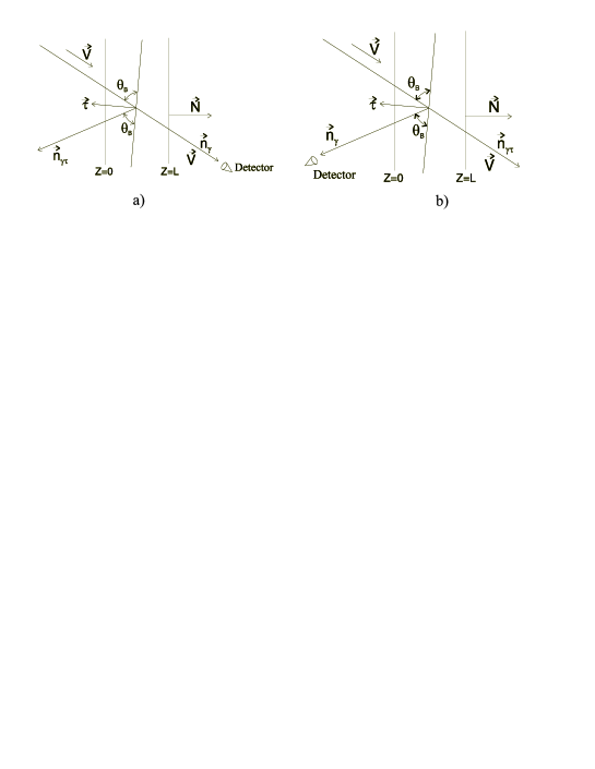
Figure 1: Schemes of diffraction geometries: a) Forward maximum, b) Diffracted maximum.

Matching the solutions of Maxwell’s equations on the crystal surface by use (4), (6) and (8), one can obtain the following expression:

$$\vec{E}_{\vec{k}}^{(-)s}(\vec{r})=\vec{e}^{s}\left[-\sum_{\mu=1}^{2}\gamma_{\mu s}^{0\ast}e^{-i\frac{\omega}{c\gamma_{0}}\varepsilon_{\mu s}^{\ast}L}\right]e^{i\vec{k}\vec{r}}\Theta(-z)+$$

$$\left\{\vec{e}^{s}\left[-\sum_{\mu=1}^{2}\gamma_{\mu s}^{0\ast}e^{-i\frac{\omega}{c\gamma_{0}}\varepsilon_{\mu s}^{\ast}(L-z)}\right]e^{i\vec{k}\vec{r}}+\vec{e}_{\tau}^{s}\beta_{1}\left[\sum_{\mu=1}^{2}\gamma_{\mu s}^{\tau\ast}e^{-i\frac{\omega}{c\gamma_{0}}\varepsilon_{\mu s}^{\ast}(L-z)}\right]e^{i\vec{k}_{\tau}\vec{r}}\right\}\Theta(L-z)\Theta(z)+$$

$$\left\{\vec{e}^{s}e^{i\vec{k}\vec{r}}+\vec{e}_{\tau}^{s}\beta_{1}\left[\sum_{\mu=1}^{2}\gamma_{\mu s}^{\tau\ast}e^{-i\frac{\omega}{c\gamma_{0}}\varepsilon_{\mu s}^{\ast}L}\right]e^{i\vec{k}_{\tau}\vec{r}}\right\}\Theta(z-L),$$ (9)

where

$$\gamma_{1(2)s}^{0} = \frac{2\varepsilon_{2(1)s}-\chi_{0}}{(2\varepsilon_{2(1)s}-\chi_{0})-(2\varepsilon_{1(2)s}-\chi_{0})\exp(-i\frac{\omega}{c\gamma_{0}}(\varepsilon_{2(1)s}-\varepsilon_{1(2)s})L)}$$

$$\gamma_{1(2)s}^{\tau} = \frac{-\beta_{1}C_{s}\chi_{\tau}}{(2\varepsilon_{2(1)s}-\chi_{0})-(2\varepsilon_{1(2)s}-\chi_{0})\exp(-i\frac{\omega}{c\gamma_{0}}(\varepsilon_{2(1)s}-\varepsilon_{1(2)s})L)}.$$ (10)

According to (4) in case of two-beam diffraction there are two different refraction indices for photons propagating inside a crystal and one of them being able to become greater than unit. That is, the superposition of slow and fast waves propagates in a crystal. The important thing is that the refraction indices for both waves strongly depend on frequencies and propagation directions of photons.

Substituting (9) in (3) one can obtain the differential number of PXR quanta with polarization vector $\vec{e}_{s}$ diffracted forwards for the Bragg case:

$$\frac{d^{2}N_{s}}{d\omega d\Omega}=\frac{e^{2}Q^{2}\omega}{4\pi^{2}\hbar c^{3}}(\vec{e}_{s}\vec{v})^{2}\left|\sum_{\mu=1,2}\gamma_{\mu s}^{0}e^{i\frac{\omega}{c\gamma_{0}}\varepsilon_{\mu s}L}\left[\frac{1}{\omega-\vec{k}\vec{v}}-\frac{1}{\omega-\vec{k}_{\mu s}\vec{v}}\right]\left[e^{\frac{i(\omega-\vec{k}_{\mu s}\vec{v})L}{c\gamma_{0}}}-1\right]\right|^{2},$$ (11)

here $\vec{e}_{1}||\left[\vec{k}\vec{\tau}\right]$ , $\vec{e}_{2}||\left[\vec{k}\vec{e}_{1}\right]$ , $\vec{k}_{\mu s}=\vec{k}+\frac{\omega}{c\gamma_{0}}\varepsilon_{\mu s}\vec{N}$.

For PXR quanta with the polarization vector $\vec{e}_{\tau s}$ diffracted at a large angle relative to the charged particle velocity the above formula can be rewritten as follows:

$$\frac{d^{2}N_{s}}{d\omega d\Omega}=\frac{e^{2}Q^{2}\omega}{4\pi^{2}\hbar c^{3}}(\vec{e}_{\tau s}\vec{v})^{2}\left|\sum_{\mu=1,2}\gamma_{\mu s}^{\tau}\left[\frac{1}{\omega-\vec{k}_{\tau}\vec{v}}-\frac{1}{\omega-\vec{k}_{\mu\tau s}\vec{v}}\right]\left[e^{\frac{i(\omega-\vec{k}_{\mu\tau s}\vec{v})L}{c\gamma_{0}}}-1\right]\right|^{2}.$$ (12)

2 Transition radiation and PXR

Let us compare the obtained formulae with the well-known ones for x-ray radiation transition in amorphous medium. The TXR formula is known as follows:

$$\frac{d^{2}N_{s}}{d\omega d\Omega}=\frac{e^{2}Q^{2}\omega}{4\pi^{2}\hbar c^{3}}(\vec{e}_{s}\vec{v})^{2}\left|e^{i\frac{\chi_{0}\omega}{2c\gamma_{0}}L}\left[\frac{1}{\omega-\vec{k}\vec{v}}-\frac{1}{\omega-\vec{k}_{a}\vec{v}}\right]\left[e^{\frac{i(\omega-\vec{k}_{a}\vec{v})L}{c\gamma_{0}}}-1\right]\right|^{2},$$ (13)

where $\vec{k}_{a}=\vec{k}+\frac{\omega\chi_{0}}{2c\gamma_{0}}\vec{N}$  is the photon wave vector in amorphous medium. In amorphous medium or in a crystal away from the diffraction conditions the only single wave propagates. But as a result of diffraction a coherent superposition of several waves propagates in a crystal. One can see that (13) is very similar to the expression describing PXR. When the frequencies and angles in (11) do not satisfy the diffraction conditions, the formula for forward PXR turns to the TXR one (13). At the same time the spectral-angular intensity (12) appears to be equal to zero, that is quite obvious since no diffraction at a large angle arises.

3 PXR at small angles with respect to particle’s velocity in Bragg geometry.

The expression for PXR angular distribution in forward direction can be derived from (11) using some assumptions. First of all it should be noted that $\chi_{0}<0$ and from (6) one can obtain that only one root of $\varepsilon_{\mu s}$  gives the refractive index $n>1$. As a result, the difference ($\omega-\vec{k}_{\mu s}\vec{v}$) for this $\mu$ can be equal to zero and the term in (11) containing this difference will grow proportionally to $L$. On the other hand, the term in (11) containing the same difference ($\omega-\vec{k}_{\mu s}\vec{v}$) for the other root will not be proportional to $L$, because this difference can never turn to zero. At the first glance it means that the term containing the first difference as well as for the Laue case gives the principle contribution to the radiation intensity when the particle waylength in crystal $L_{0}$ grows. But the distinctive feature of Bragg case is the possibility of total reflection of quanta that is stipulated by existence of the nonhomogeneous wave in a crystal. So, as a result, the both roots of $\varepsilon_{\mu s}$ should be considered. Therefore, to obtain the PXR angular distribution it is necessary to perform the numerical integration of (11) over frequencies in the vicinity of $\omega_{B}$.

Assuming that  $L_{0}>>l$ ($l=\lambda\gamma^{2}$ is the vacuum coherent length, $\lambda$ is wave length of the photon) and neglecting the imaginary parts of crystal susceptibilities and possible total reflection we can obtain the approximate expression for PXR angular distribution in forward direction:

$$\frac{dN_{0s}}{d\Omega} = \frac{e^{2}\vartheta^{2}}{4\pi\hbar c^{3}}\left[\begin{array}[]{c}\sin^{2}\varphi\\ \cos^{2}\varphi\end{array}\right]\frac{\beta_{1}r_{s}^{{}^{\prime}2}\left|(\gamma^{-2}-\chi_{0}^{{}^{\prime}}+\vartheta^{2})^{2}-\left|\beta_{1}\right|r_{s}^{{}^{\prime}}\right|}{(\gamma^{-2}-\chi_{0}^{{}^{\prime}}+\vartheta^{2})^{2}}\frac{\omega_{B}L_{0}}{\sin^{2}\theta_{B}}\cdot$$ (17)

$$\left|\frac{\exp(-i\omega_{B}L_{0}\frac{(\gamma^{-2}-\chi_{0}^{{}^{\prime}}+\vartheta^{2})^{2}-\left|\beta_{1}\right|r_{s}^{{}^{\prime}}}{2c(\gamma^{-2}-\chi_{0}^{{}^{\prime}}+\vartheta^{2})^{2}})}{\left|\beta_{1}\right|r_{s}^{{}^{\prime}}\exp(-i\omega_{B}L_{0}\frac{(\gamma^{-2}-\chi_{0}^{{}^{\prime}}+\vartheta^{2})^{2}-\left|\beta_{1}\right|r_{s}^{{}^{\prime}}}{2c(\gamma^{-2}-\chi_{0}^{{}^{\prime}}+\vartheta^{2})^{2}})-(\gamma^{-2}-\chi_{0}^{{}^{\prime}}+\vartheta^{2})^{2}}\right|^{2}.$$

We have investigated two geometries for PXR observation in Bragg case in forward direction.

1. As one can see from (14), maximum in angular distribution expression is reached at condition

$$\omega_{B}L_{0}\frac{(\gamma^{-2}-\chi_{0}^{{}^{\prime}}+\vartheta^{2})^{2}-\left|\beta_{1}\right|r_{s}^{{}^{\prime}}}{2c(\gamma^{-2}-\chi_{0}^{{}^{\prime}}+\vartheta^{2})^{2}}=2\pi n,\ \ n=0,1,...$$ (18)

and the beats over polar angle  $\vartheta$ may be observed. Obviously it is possible to choose a geometry where these effects would be the most essential. Fig.2 demonstrates the experimental scheme realizing the above condition.

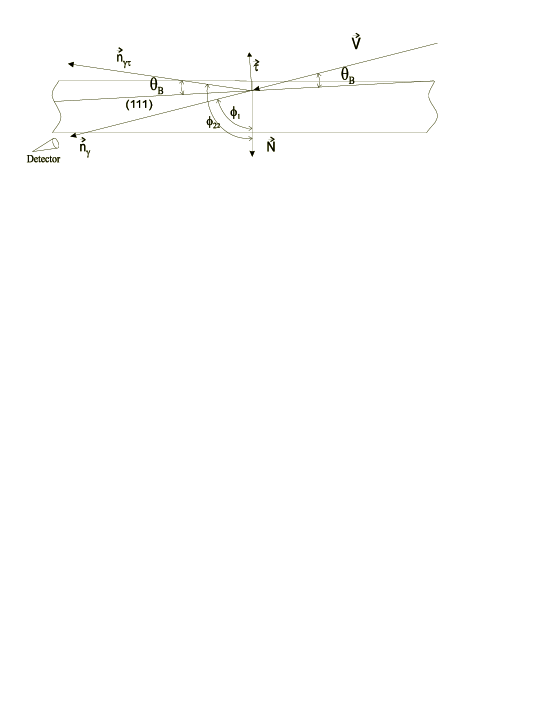
Figure 2: Geometry for observation of beating in PXR angular distribution; $\gamma_{0}=\cos\phi_{1},\gamma_{1}=\cos\phi_{2}$.

We have carried out calculations for Si and LiH crystals.Experimental parameters are given in table 1. All calculations were performed for azimuth angle $\varphi=\pi/2$ (this corresponds to $\sigma$-polarization of PXR) and diffraction plane (111).

Table 1: Experimental parameters.

N	Crystal	Diffraction plane	$\omega_{B}$,keV	$\gamma_{0}$	$\beta_{1}$	$L_{0}$, cm	$L_{br}$, cm	$L_{abs}$, cm
1	Si	(111)	30	0,1211	-11,57	8,26$\cdot$10-2	9,33$\cdot$10-3	0,362
2	Si	(111)	30	0,1177	-8,43	8,50$\cdot$10-2	9,33$\cdot$10-3	0,362
3	Si	(111)	30	0,1142	-6,55	8,76$\cdot$10-2	9,33$\cdot$10-3	0,362
4	Si	(111)	30	0,1055	-4,03	9,48$\cdot$10-2	9,33$\cdot$10-3	0,362
5	Si	(111)	30	0,0882	-2,02	1,13$\cdot$10-1	9,33$\cdot$10-3	0,362
6	Si	(111)	30	0,0659	-1,00	1,52$\cdot$10-1	9,33$\cdot$10-3	0,362
7	Si	(111)	30	0,0349	-0,36	2,87$\cdot$10-1	9,33$\cdot$10-3	0,362
8	Si	(111)	20	0,1636	-4,85	3,06$\cdot$10-3	1,14$\cdot$10-2	0,106
9	Si	(111)	20	0,1636	-4,85	3,06$\cdot$10-2	1,14$\cdot$10-2	0,106	*
10	LiH	(111)	15	0,3292	-20,10	3,04$\cdot$10-2	4,60$\cdot$10-2	17,4
11	LiH	(111)	20	0,2507	-25,35	3,99$\cdot$10-2	3,98$\cdot$10-2	41,1	*
12	LiH	(111)	30	0,1707	-46,71	5,86$\cdot$10-2	3,25$\cdot$10-2	139

Fig.3 demonstrates spectral-angular distribution of parametric x-radiation for experimental parameters shown in the 8-th row of table 1. In this geometry PXR is generated within frequency range where the coefficient characterizing the efficiency of X-ray reflection by the atomic planes becomes nearly equal to unit. In fig.3 the right part of spectrum is a flat curve - this is the range of total Bragg reflection.

Figure 3: Spectral-angular distribution of PXR for polar angle $\vartheta=2,09$ mrad (azimuth angle $\varphi=\pi/2$). 1 - without multiple scattering (MS) taken into account, 2 - with MS.

The angular distribution for geometry described by the 3-d row of table 2 is shown in fig.4. The curve 1 is derived by integration of spectral-angular distribution over the frequency range $\Delta\omega/\omega_{B}=10^{-4}$ within $\omega_{0}$, corresponding to the center of PXR diffraction maximum for each pair $(\varphi,\vartheta)$. The curve 2 is given by (14), it shows more pronounced beating over polar angle than curve 1. The maxima of angular distribution for analytical formula exceed the maximum values of distribution obtained by integration. This can be explained by more exact account of absorption effect while performing integration of spectral-angular distribution. Analytical formula was obtained with some assumptions (neglecting of imaginary parts of crystal susceptibilities) that leads to some overestimation of PXR angular intensity.

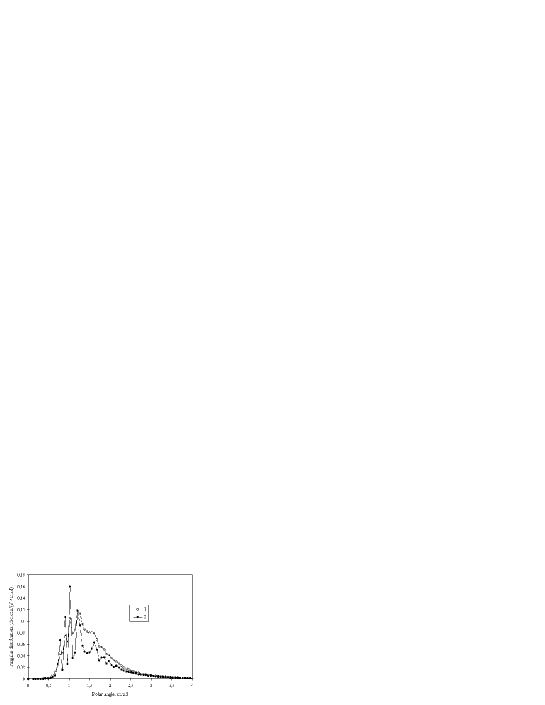
Figure 4: Angular distribution of PXR derived on the base of: 1- integration of spectral-angular distribution over frequencies, 2 - analytical formula for angular distribution.

Fig.5 demonstrates angular distributions of PXR for different values of geometrical factor $\beta_{1}$ – first seven rows of table 1 (this corresponds to different angles between (111) plane and surface of crystal plate).

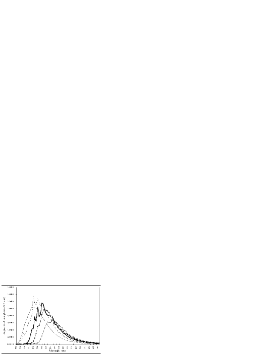
Figure 5: PXR angular distributions for different values of $\beta_{1}$ factor (from the left $\beta_{1}=-2,02;-4,03;-6,55;8,43;-11,57$.

2. Another variant of experimental geometry is given by scheme shown in fig. 6. The Bragg angle $\theta_{B}$ is equal to 90 degrees, this is the geometry realizing normal incidence of particles on diffraction plane, the surface of crystal plate is parallel to diffraction planes.

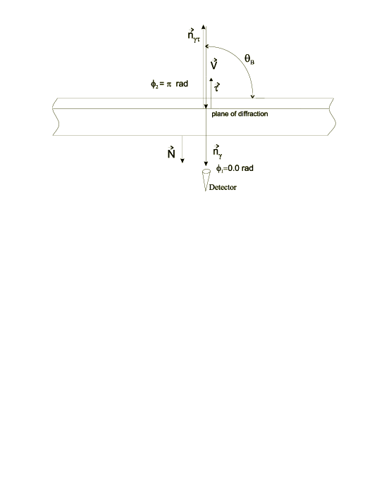
Figure 6: Experimental geometry realizing perpendicular incidence.

The calculations for the experimental parameters presented in table 2 were carried out .

Table 2: Experimental parameters.

N	Crystal	Diffraction plane	$\omega_{B}$,keV	$\gamma_{0}$	$\beta_{1}$	$L_{0}$, cm	$L_{br}$, cm	$L_{abs}$, cm
1	Si	(555)	9,887	1,00	-1,00	0,05	$1,63\cdot 10^{-2}$	$1,28\cdot 10^{-2}$
2	Si	(555)	9,887	1,00	-1,00	0,01	$1,63\cdot 10^{-2}$	$1,28\cdot 10^{-2}$	*
3	Si	(555)	9,887	1,00	-1,00	0,005	$1,63\cdot 10^{-2}$	$1,28\cdot 10^{-2}$
4	LiH	(333)	7,876	1,00	-1,00	0,05	$6,35\cdot 10^{-2}$	2,52	*
5	LiH	(333)	7,876	1,00	-1,00	0,01	$6,35\cdot 10^{-2}$	2,52
6	LiH	(333)	7,876	1,00	-1,00	0,005	$6,35\cdot 10^{-2}$	2,52

The spectral-angular distribution for geometry corresponding to the 3-d row of table 2 is shown in fig.7.

Figure 7: Spectral-angular distributions of PXR for polar angle $\vartheta=12,23mrad$ (azimuth angle) $\varphi=\pi/2$ 1 – without account of MS; 2 – with account of MS.

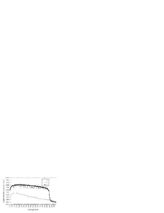
Figure 8: Angular distributions of PXR obtained on the base of: 1 - analytical formula for angular intensity, 2 - integrating spectral-angular distribution over frequencies ($\Delta\omega/\omega_{B}=10^{-4}$) without taking into account multiple scattering, 3 - integrating spectral-angular distribution over frequencies ($\Delta\omega/\omega_{B}=10^{-4}$) taking into account multiple scattering.

Fig.8 presents PXR angular distribution corresponding to the 3-d row of table 2. Such essential difference between results obtained on the base of analytical formula and that of integration of spectral-angular distribution can be explained by the fact that the formula (14) does not take into account the nonhomogeneous waves arising at the total reflection in Bragg case (in contrast with Laue geometry where the total reflection does not realized) (see fig. 7 – the flat part of spectral-angular distribution curve).

4 PXR at large angles with respect to particle’s velocity.

As well as for forward PXR, in order to obtain angular distribution for diffracted PXR (see fig.1, (b)) taking into account the effect of absorption, possible total reflection of quanta in a crystal and contribution of both slow and fast waves in radiation intensity it is necessary to perform the numerical integration of spectral-angular distribution (12) over frequencies in the vicinity of $\omega_{B}$. We have carried out calculations for the geometry presented in fig.9.

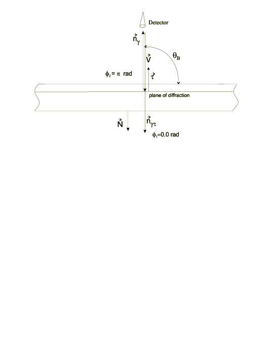
Figure 9: Geometry of backward diffraction.

Figure 10: Spectral-Angular distribution for backward diffraction in Si crystal, diffraction plane (111), particle’s energy 86,9 MeV, $\vartheta=18,6$ mrad (azimuth angle $\varphi=\pi/2$ ), $\omega_{B}=1,98keV$, $L=1,25\cdot 10^{-3}$ cm. 1 – PXR spectral-angular distribution (SAD) for the first dispersion branch $\mu=1$ without the terms proportional to $\frac{1}{\omega-\vec{k}\vec{v}}$; 2 – SAD for $\mu=2$ without the terms proportional to $\frac{1}{\omega-\vec{k}\vec{v}}$; 3 – SAD for the both dispersion branches without the terms $\frac{1}{\omega-\vec{k}\vec{v}}$; 4 – SAD for the both dispersion branches without the terms proportional to $\frac{1}{\omega-\vec{k}_{\mu s}\vec{v}}$; 5 – SAD described by the formula (12).

Figure 11: Angular distribution for backward diffraction, derived by integration (12) over frequencies in the range $\Delta\omega/\omega_{B}=10^{-3}$ in silicon crystal for azimuth angle $\varphi=\pi/2$, diffraction plane (111), particle’s energy 86,9 MeV, $\omega_{B}=1,98$ keV, $L=1,25\cdot 10^{-3}$ cm. 1– PXR angular distribution for the both dispersion branches without integration the terms proportional to $\frac{1}{\omega-\vec{k}\vec{v}}$; 2– PXR angular distribution with taking into account during integration all terms in expression (12).

Figure 12: Angular distribution for backward diffraction, in silicon crystal for azimuth angle $\varphi=\pi/2$, diffraction plane (400), particle’s energy 80,5 MeV, $\omega_{B}=4,57$ keV, $L=1,25\cdot 10^{-3}$ cm. a – results of [19]; b – derived by integration (12) over frequencies in the range $\Delta\omega/\omega_{B}=10^{-3}$

Figs. 10 and 11 show spectral-angular and angular distributions for backward diffraction. How one can see from Fig.12, expression (12), taking into account effects of a dynamic diffraction, allows to describe the experiment more precisely than the formula of the kinematic theory [15].

5 Effect of multiple scattering on PXR.

In addition to absorption of photons in crystalline plate multiple scattering of charged particles by atoms of crystal is the other essential factor also leading to limitation of longitudinal dimensions of PXR generation range. So, the PXR characteristics strongly depend on relation between crystal thickness $L_{0}$ and coherent length of bremsstrahlung radiation $L_{br}$. When $L_{0}<<L_{br}$ the influence of multiple scattering reduces actually to a small addition to PXR intensity due to bremsstrahlung radiation mechanism. In the opposite case, when $L_{0}>L_{br}$, multiple scattering significantly changes PXR parameters. The calculations taking into account multiple scattering effect were carried out on the base of expressions given in [7].

The relation between $L_{br}$ and crystal thickness $L_{0}$ determines the influence of multiple scattering on PXR characteristics (the values $L_{br}$ are contained in the 8-th columns of tables 1 and 2) Figs. 3, 7, 8 represents PXR (spectral-angular and angular) distributions taking into account multiple scattering influence. All these distributions were obtained for thin crystalline plates ($L$ $<L_{br}$).

In fig.13 angular distributions of PXR and bremsstrahlung radiation caused by multiple scattering for the parameters presented in the 3-d row of table 1 are shown. These distributions were obtained by integration of spectral-angular distributions while taking multiple scattering into account and without it. This is the case of intense MS, $L_{0}\sim 9$ $L_{br}$, MS leads to strong reduction of PXR intensity.

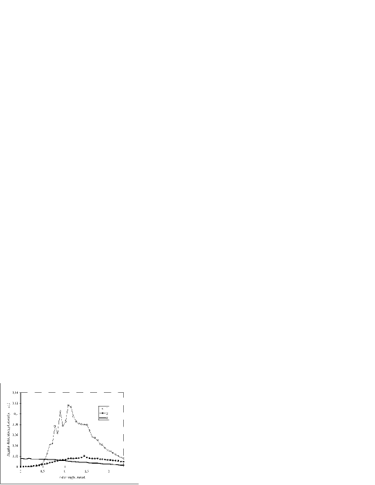
Figure 13: PXR angular distribution in silicon crystal: 1 – PXR without account of MS; 2 – PXR with account of MS; 3 – Bremsstrahlung caused by MS.

Figure 14: PXR angular distribution in silicon crystal with account of MS: 1 – $L=0,005$ cm, 2 – $L=0,01$ cm, 3 – $L=0,05$ cm.

Fig.14 demonstrates dependence of intensity of angular distribution on the thickness of crystalline plate. The parameters describing these situations are given in rows 1-3 of table 2. For plate of thickness $L_{0}=0,005$ cm MS is not very essential (see fig. 7), for thickness of 0,01 cm ($L_{0}\sim L_{br}$) MS is already noticeable, and in plate with the thickness of 0,05 cm MS plays the important role in PXR intensity reduction.

6 PXR in LiH crystall.

Use in experiments of LiH crystal enables to realize weak MS even for sufficiently thick crystals (see rows 11 and 12 of table 1 and rows 4, 5, 6 of table 2). In case of Bragg diffraction for geometry described by fig.2 it is possible to observe beating over polar angle in angular distributions measurements. The experimental geometries more advantageous for PXR observation are marked in table 1 by (*). For these experimental schemes the comparison between angular intensities of PXR and TXR was carried out ($\Delta\omega/\omega_{B}=10^{-4}$). Figure 15 demonstrates angular distributions of PXR and TXR for LiH crystal.

For Bragg diffraction in case of normal incidence the geometries preferable for PXR observation possibility are asterisked at margins of table 2.

Fig.16 demonstrates comparison of PXR and TXR angular intensities for situation described by the 4-th row of table 2.

Figure 15: Angular distribution in LiH crystal for geometry described by fig.2: 1 – PXR, 2 – TXR.

Figure 16: Angular distribution in LiH crystal, case of normal incidence geometry: 1 - PXR, 2 - TXR. $\omega_{B}=7,88$ keV, $L_{0}=0,01$ cm.

Conclusion.

The only precision account of all dynamic effects (total Bragg reflection, interference of slow and fast waves or, by the other words, taking into consideration of all terms in (12), allows to obtain the real picture of diffraction radiation in case of Bragg geometry. The contributions of both the slow and the fast waves in radiation intensity for Bragg geometry are comparable and only their joint account allows to describe the experimental results.

References

• [1] V.G.Baryshevsky, Dokl. Akad. Nauk BSSR. 15 (1971) 306.
• [2] V.G.Baryshevsky, I.D. Feranchuk, Sov.Phys.JETP. V64. N3(9) (1971) 944, V64. N2 (1973) 760.
• [3] Yu.N.Adishchev, V.G.Baryshevsky et al., Lett.J.ExpTheor.Phys.(Soviet) 41 (1985) 259.
• [4] V.G.Baryshevsky et al., Phys.Lett. A110 (1985) 477; Phys.Lett. A110 (1985) 177
• [5] V.G.Baryshevsky et.al. Nucl.Instr.and Meth. Phys.Res. A249(1986) 304.
• [6] Y.N.Adishchev et.al., Nucl.Instr. Meth. Phys.Res., B44, (1989) 130.
• [7] V.G.Baryshevsky, A.O.Grubich, Le Tien Hai. Sov.Phys.JETP. V24. N5, (1988) 51.
• [8] G.M.Garibian and J.Shee, Zh. Eksp. Teor. Fiz. 63(1972) 1198 [Sov. Phys. JETP 36 (1973) 631].
• [9] V.G.Baryshevsky, I.D. Feranchuk, Phys. Lett. A57.(1976) 183.
• [10] V.G.Baryshevsky, Feranchuk I.D. J. Physique. V44, N8,(1983) 913.
• [11] A.Caticha, Phys. Rev. A40 (1989) 4322; Phys. Rev. B45 (1992) 9541.
• [12] H.Nitta, Phys.Lett. A158 (1991) 270; Phys. Rev. B45 (1992) 7621.
• [13] R.F.Fiorito et.al. Nucl.Instr. Meth. in Phys.Res, B79 (1993) 758; Phys.Rev. E51 (1995) R2759.
• [14] J. Freudenberger et.al., Phys. Rev. Lett., 74 (1995) 2487.
• [15] M.L.Ter-Mikaelian, High-Energy Electromagnetic Processes in Condenced Media. (Wiley, New York, 1972).
• [16] V.G.Baryshevsky. Nucl.Instr. and Meth. B122 (1997) 13.
• [17] Z.G.Pinsker, Dynamic Dispersion in Perfect Crystals. (Nauka, Moscow, 1974).
• [18] Shin-Lin Chang, Multiple Diffraction of X-rays in Crystals (Springer, Berlin, 1984).
• [19] J. Freudenberger et.al.,Parametric X Radiation and Approaches to Application. 198. WE - Heraeus-Seminar, June 09-12 in Tabarz/Germany.