Measurement of $W$ and $Z$ boson production cross sections

Abstract

DØ has measured the inclusive production cross section of $W$ and $Z$ bosons in a sample of 13 pb^-1 of data collected at the Fermilab Tevatron. The cross sections, multiplied by their leptonic branching fractions, for production in $p\bar{p}$ collisions at $\sqrt{s}$ = 1.8 TeV are $\sigma_{W}{\rm B}({\mbox{$W\rightarrow e\nu$}})=2.36\pm 0.02\pm 0.08\pm 0.13{\rm~{}nb}$, $\sigma_{W}{\rm B}({\mbox{$W\rightarrow\mu\nu$}})=2.09\pm 0.06\pm 0.22\pm 0.11{\rm~{}nb}$, $\sigma_{Z}{\rm B}({\mbox{$Z\rightarrow{e^{+}e^{-}}$}})=0.218\pm 0.008\pm 0.008\pm 0.012{\rm~{}nb}$, and $\sigma_{Z}{\rm B}({\mbox{$Z\rightarrow{\mu^{+}\mu^{-}}$}})=0.178\pm 0.022\pm 0.021\pm 0.009{\rm~{}nb}$, where the first uncertainty is statistical and the second systematic; the third reflects the uncertainty in the integrated luminosity. For the combined electron and muon analyses, we find ${\sigma_{W}{\rm B}(W\rightarrow l\nu)}/{\sigma_{Z}{\rm B}(Z\rightarrow l^{+}l^{-})}=10.90\pm 0.52$. Assuming standard model couplings, we use this result to determine the width of the $W$ boson, and obtain $\Gamma(W)=2.044\pm 0.097\;{\rm GeV}$.

I Introduction

Measurement of the production cross sections multiplied by the leptonic branching fractions ($\sigma{\rm B}$) for $W$ and $Z$ bosons can be used to test predictions of QCD for $W$ and $Z$ production, and to extract the width of the $W$ boson. Previous measurements of these cross sections have been made at $\sqrt{s}=630$ GeV by the UA1 [3] and UA2 [4] experiments and at $\sqrt{s}=1.8$ TeV by CDF [5, 6, 7, 8, 9]. The results reported in this paper are from the DØ detector, operating at $\sqrt{s}=1.8$ TeV, and have been summarized previously in Ref. [10].

Precise determination of the total widths of the $W$ and $Z$ bosons provides an important test of the standard model because these widths are sensitive to new (and possibly undetected) decay modes. The total width of the $Z$ boson is known to a precision of $0.3\%$ [11] which places strong constraints on the existence of any new particles that can contribute to decays to neutrals. Our knowledge of the total width of the $W$ boson is an order of magnitude less precise, and the corresponding limits on charged weak decays are much less stringent. It is therefore important to improve the measurement of the width of the $W$ boson as a means of searching for any unexpected $W$-boson decay modes.

We determine the width of the $W$ boson indirectly by using the ratio of the measured $W$ and $Z$ boson $\sigma{\rm B}$ values

$$R \equiv {{\sigma_{W}{\rm B}(W\rightarrow l\nu)}\over{\sigma_{Z}{\rm B}(Z\rightarrow ll)}},$$

where $l$ corresponds to $e$ or $\mu$, $\sigma_{W}$ and $\sigma_{Z}$ are the inclusive cross sections for $W$ and $Z$ boson production, $\sigma(p\bar{p}\to W+X)$ and $\sigma(p\bar{p}\to Z+X)$, and ${\rm B}(W\rightarrow l\nu)$ and ${\rm B}(Z\rightarrow ll)$ are the leptonic branching fractions of the $W$ and $Z$ bosons. We extract ${\rm B}(W\rightarrow l\nu)$ from the above ratio using a theoretical prediction for $\sigma_{W}/\sigma_{Z}$, and the precise measurement of ${\rm B}(Z\rightarrow ll)$ from LEP. We then combine ${\rm B}(W\rightarrow l\nu)$ with the leptonic partial width ${\Gamma(W\rightarrow l\nu)}$ to obtain the total width of the $W$ boson, $\Gamma(W)$.

Many of the systematic uncertainties (both experimental and theoretical) that affect the determination of the individual cross sections $\sigma_{W}{\rm B}(W\rightarrow l\nu)$ and $\sigma_{Z}{\rm B}(Z\rightarrow ll)$ cancel when calculating the ratio $R$. At the present time, $R$ gives the best determination of $\Gamma(W)$; direct measurements from fits to the tail of the transverse mass distribution of the $W$ boson are currently four times less precise [13], but require fewer standard model assumptions.

In this paper, we report results of the measurement of the $W$ and $Z$ production cross sections, and the extraction of $\Gamma(W)$, using data collected in the first collider run of the DØ detector starting in August 1992 and ending in June 1993. During the run, the Tevatron operated with a typical instantaneous luminosity of $4.0\times 10^{30}$ cm^-2s^-1 and a peak luminosity of $9.7\times 10^{30}$cm^-2s^-1. DØ recorded to tape a total of $\sim 13$ pb^-1 of data.

II The DØ Detector

DØ is a multipurpose detector designed to study $p\bar{p}$ collisions at the Fermilab Tevatron Collider. It consists of three primary components: a nonmagnetic central tracking system, a nearly hermetic uranium/liquid-argon calorimeter, and a magnetic muon spectrometer. A cutaway view of the detector is shown in Fig. 1. A full description can be found in Ref. [14]; below we give details of the detector relevant to this analysis.

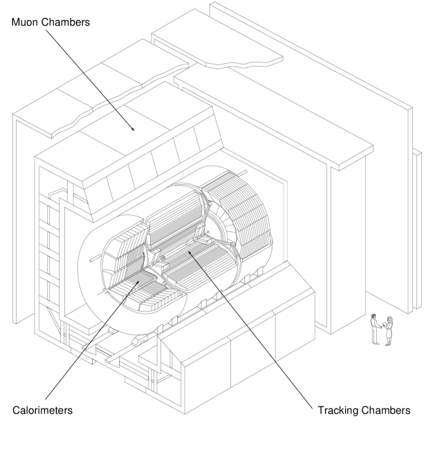
FIG. 1.: Cutaway isometric view of the DØ detector.

A Central Tracking System

The central tracking system consists of four detector subsystems: a vertex drift chamber (VTX), a transition radiation detector (TRD), a central drift chamber (CDC), and two forward drift chambers (FDC). The system provides charged-particle tracking over the pseudorapidity region $|\eta|<3.2$, where $\eta=\tanh^{-1}(\cos\theta)$, $\theta$ is the polar angle, and $\phi$ is the azimuthal angle. Trajectories of charged particles are measured with a resolution of 2.5 mrad in $\phi$ and 28 mrad in $\theta$. From these measurements, the position of the interaction vertex along the beam direction ($z$) can be determined with a typical resolution of 8 mm. The central tracking system also measures the ionization of tracks, and can be used to distinguish single charged particles and $e^{+}e^{-}$ pairs from photon conversions.

B Calorimeter

Surrounding the central tracking system is the calorimeter, which is divided into three parts: a central calorimeter (CC) and two end calorimeters (EC). They each consist of an inner electromagnetic (EM) section, a fine hadronic (FH) section, and a coarse hadronic (CH) section, housed in a steel cryostat. The intercryostat detector (ICD) consists of scintillator tiles inserted in the space between the EC and CC cryostats. The ICD improves the energy resolution for jets that straddle two cryostats. The calorimeter covers the range $|\eta|<4.2$.

Each EM section is 21 radiation lengths deep, and is divided into four longitudinal segments (layers). The hadronic sections are 7–9 nuclear interaction lengths deep, and are divided into four (CC) or five (EC) layers. The calorimeter is transversely segmented into pseudoprojective towers of $\Delta\eta\times\Delta\phi$ = $0.1\times 0.1$. The third layer of the EM calorimeter, in which the maximum energy deposition of EM showers is expected, is segmented twice as finely into cells with $\Delta\eta\times\Delta\phi$ = $0.05\times 0.05$. With this fine segmentation, the position resolution for electrons above 50 GeV in energy is about 2.5 mm. The energy resolution is $\sigma(E)/E=15\%/\sqrt{E\hbox{(GeV)}}\oplus 0.4\%$ for electrons. For charged pions the resolution is about $50\%/\sqrt{E\hbox{(GeV)}}$, and for jets about $80\%/\sqrt{E\hbox{(GeV)}}$ [14]. From minimum-bias data, for the imbalance in transverse momentum, or “missing $E_{T}$”(see Sec. III C), or $\hbox to0.0pt{\kern 2.5pt/\hss}E_{T}$, the resolution for each component ($\hbox to0.0pt{\kern 2.5pt/\hss}E_{x}$ and $\hbox to0.0pt{\kern 2.5pt/\hss}E_{y}$) is $1.08\hbox{ GeV}+0.019(\Sigma E_{T})$, where $\Sigma E_{T}$ is the scalar sum of the transverse energies over all calorimeter cells.

The readout of the individual calorimeters cells are subject to zero suppression. They are read out only if the signal is outside of a two-standard-deviations window centered on the mean of the noise.

C Muon Spectrometer

Outside the calorimeter, there are muon detection systems covering $|\eta|\leq 3.3$. Since muons from $W$ and $Z$ boson decays populate predominantly the central region, this work uses only the wide angle muon spectrometer (WAMUS), which consists of four planes of proportional drift tubes (PDT) in front of magnetized iron toroids with a magnetic field of 1.9 T, and two groups of three planes each of proportional drift tubes behind the toroids. The magnetic field lines and the wires in the drift tubes are oriented transversely to the beam direction. The WAMUS covers the region $|\eta|<1.7$ over the entire azimuth, with the exception of the central region below the calorimeter ($|\eta|<1$, $225^{\circ}<\phi<315^{\circ}$), where the inner layer is missing to make room for the support structure of the calorimeter.

The total material in the calorimeter and iron toroids varies between 13 and 19 interaction lengths, making background in the muon chambers from hadronic punchthrough negligible. The DØ detector is significantly more compact than previous magnetic $p\bar{p}$ collider detectors [15, 16], and the small tracking volume reduces backgrounds from muons from inflight decays of $\pi$ and $K$ mesons.

The muon momentum $p$ is measured from the muon deflection angle in the magnetic field of the toroid. The momentum resolution is limited by multiple scattering in the traversed material, knowledge of the magnetic field, and measurement of the deflection angle. The resolution in $1/p$ is approximately Gaussian and given by $\sigma(1/p)=0.18(p-2)/p^{2}\oplus 0.008$ (with $p$ in GeV) for the algorithm that was used to select the data presented here. The first of the two components in the above resolution function arises from multiple-Coulomb scattering in the iron toroids, and is the dominant effect for low-momentum muons. The second component is from the resolution on the measurement of the muon trajectory.

III Particle Identification and Event Selection

Because it is more difficult to separate the hadronic decays of $W$ and $Z$ bosons from the large background of dijet production, the cross section analysis uses the leptonic decay modes, $W\rightarrow l\nu$ and $Z\rightarrow ll$ with $l=e$ [17], $\mu$ [18].

The leptonic decays are characterized by a high-$p_{T}$ lepton and large $\hbox to0.0pt{\kern 2.5pt/\hss}E_{T}$ or by two high-$p_{T}$ leptons, for $W$ or $Z$ boson decays, respectively. This section describes the identification criteria used for electrons, muons, and neutrinos in this analysis.

A Events with Electrons

Electrons are identified primarily by the presence of an electromagnetic shower in the calorimeter. A clustering algorithm finds these showers, and quality criteria are used to pick out electrons and photons, and thereby reduce backgrounds. Information from the central tracking system is used to separate electrons from photons.

This analysis considers electrons in the Central Calorimeter (CC) defined by $|\eta|\leq 1.1$, and the End Calorimeters (EC), $1.5\leq|\eta|\leq 2.5$. The region between the calorimeters is excluded because of poor resolution. In the CC, we also exclude electrons within 0.01 radians in $\phi$ of the crack between adjacent calorimeter modules.

1 Clustering Algorithm

A nearest-neighbor cluster-finding algorithm [19] is employed to find the electromagnetic energy clusters to be associated with electrons or photons. In each $\Delta\eta\times\Delta\phi=0.1\times 0.1$ tower, we sum the energies in all layers of the EM calorimeters. We then loop over all such EM energy towers with $E>50$ MeV, and search the nearest-neighbor towers for high transverse energy. If there are other towers with $E>50$ MeV, a local connection is made between those neighboring towers. In the next step, clusters are defined as groups of connected towers. If the transverse energy of the cluster is greater than $1.5$ GeV, the cluster is saved for further analysis. The energy in the EM portion of the calorimeter is also required to exceed $90\%$ of the total energy of the cluster, and the energy outside the central tower must be less than $60\%$ of the total. Both of these requirements are chosen to select clusters corresponding to narrow EM particle showers, as expected for electrons or photons.

At this stage, the “electron” sample has a very large background from QCD processes (such as dijet production). This is because hadronic showers from QCD jets can sometimes fluctuate to look like electron or photon showers. Several other variables are introduced therefore to clean up the electron and photon selections. These variables involve a $\chi^{2}$ for the shape of the shower, the shower’s isolation, and the spatial match between the calorimetric shower and the extrapolated position of some charged track emanating from the interaction vertex.

2 Covariance Matrix for the Shower

Development of electron or photon showers in calorimeters is characteristically different from that of jets. The profile of the shower both in the longitudinal and transverse directions can therefore be used to discriminate between signal and QCD background. A covariance matrix is constructed to compare the shape of the experimentally observed shower with that expected from electrons or photons, taking into account the correlations among energy depositions in all the calorimeter cells in the cluster.

For a sample of N electrons, a covariance matrix is defined as

$$M_{ij}=\frac{1}{N}\sum_{n=1}^{N}(x_{ni}-<x_{i}>)(x_{nj}-<x_{j}>),$$ (1)

where $x_{ni}$ is the value of the $i$th observable for the $n$th electron, and $<x_{i}>$ is the sample mean for that observable. There are 41 variables in the matrix: the fractions of shower energy in EM layers 1, 2 and 4, the fraction of shower in each cell in a $6\times 6$ array centered at the hottest tower in EM layer 3, the logarithm of the shower energy, and the $z$ position of the event vertex. A matrix , based on Monte Carlo simulation of electron showers, is constructed for each of the 37 detector towers at different values of $|\eta|$. The Monte Carlo simulation was tuned to agree with the shower shapes of test beam electrons.

For showers in the data, we calculate the H-matrix $\chi^{2}$ function:

$$\chi^{2}=\sum_{ij}(x_{i}-<x_{i}>)H_{ij}(x_{j}-<x_{j}>),$$ (2)

where $x_{i}$ is the measured value of the $i$th observable, and $H=M^{-1}$. Figure 2 shows the distribution of $\chi^{2}$ for showers from electron candidates from $Z\to ee$ decays, and EM clusters in inclusive jet events that are primarily from overlaps between charged and neutral particle and $\pi^{0}$ decays. The two distributions are clearly different. Note that the covariance $\chi^{2}$ parameter will not necessarily follow a standard $\chi^{2}$ distribution, because, in general, the observables defining the matrix are not normally distributed [20]. We require that an acceptable electron shower have $\chi^{2}\leq 100$.

FIG. 2.: $\chi^{2}$ distribution for (a) electrons and (b) jets. The arrows indicate the position of the cutoff used in this analysis at $\chi^{2}=100$.

3 Isolation Parameter

An isolation variable is very useful for discriminating between background from jets and electrons from $W$ or $Z$ decay. Such electrons usually have very few other particles in their vicinity, while a jet contains many collimated particles close to each other. We therefore reject electron candidates with a significant amount of energy deposition nearby in the calorimeter.

The isolation parameter for a cluster is defined by the fraction of energy in the vicinity of the core towers of that cluster

$$f_{{\rm iso}}=\frac{E_{{\rm tot}}({\cal R}=0.4)-E_{{\rm EM}}({\cal R}=0.2)}{E_{{\rm EM}}({\cal R}=0.2)}$$ (3)

where $E_{{\rm tot}}$ is the total energy in the calorimeter in a cone with a radius ${\cal R}=\sqrt{(\Delta\eta)^{2}+(\Delta\phi)^{2}}=0.4$, and $E_{{\rm EM}}$ is the energy in the EM section in a cone with radius $0.2$. Figure 3 shows the distributions found for electrons and jets. We require that acceptable electrons satisfy $f_{{\rm iso}}<0.10$.

FIG. 3.: Distribution in the isolation fraction for (a) electrons and (b) jets. The arrows indicate the cutoff used in this analysis at $f_{\rm{iso}}=0.1$.

4 Track Matching in the Central Detector

Track information is used to distinguish electrons from photons. A reconstructed track is required to be within a $0.1\times 0.1$ cone pointing towards the centroid of the EM shower. If this requirement is satisfied, the cluster is classified as an electron candidate, otherwise it is considered as a photon candidate. A track significance is defined as a measure of the quality of the match between the track and the centroid of the shower. For the central drift chambers (CDC), it is defined as:

$$\sigma_{{\rm trk}}=\sqrt{\left(\frac{\delta z}{\sigma_{z}}\right)^{2}+\left(\frac{\delta\phi}{\sigma_{\phi}}\right)^{2}}$$ (4)

while for the forward drift chambers (FDC), it is defined as:

$$\sigma_{{\rm trk}}=\sqrt{\left(\frac{\delta\rho}{\sigma_{\rho}}\right)^{2}+\left(\frac{\delta\phi}{\sigma_{\phi}}\right)^{2}}$$ (5)

where $z,\rho$, and $\phi$ are cylindrical coordinates and all the differences ($\delta$’s) are calculated between the extrapolated coordinates of the track and the centroid of the shower in EM layer 3 of the calorimeter. The standard deviations ($\sigma$’s) in the denominators are the experimental resolutions for the corresponding matching parameters. Figure 4 shows the distributions in $\sigma_{{\rm trk}}$ for electrons and jets in the CC, and the cutoffs used to define electrons.

FIG. 4.: Significance track matching for (a) electrons in the CC and (b) jets in the CC. The arrows indicate the value of the cutoff used in this analysis at $\sigma_{\rm{trk}}=5$ in the CC.

5 Energy Scale Calibration

The absolute EM energy scale of the DØ calorimeter is determined using events in the $Z\to ee$ mass peak [21]. An initial calibration was performed based on test beam studies of electrons and pions in a prototype calorimeter module. These determined that any nonlinearity and energy offsets of the calorimeter were negligible. We set the absolute scale by measuring the $Z$ invariant mass peak and scaling our initial result to the known value of the $Z$ mass [22]. This correction is determined separately for each of the three calorimeter cryostats. The magnitude of the correction ranges from 1% to 7% [23].

6 Defining Electron Categories

We define three categories of reconstructed electrons, referred to as “tight”, “standard”, and “loose”. The tight criteria are used to reduce backgrounds as much as possible, while the loose criteria are used to obtain a higher reconstruction efficiency for electrons. The standard criteria are employed in the measurement of electron efficiencies.

Tight electrons are defined as reconstructed EM clusters that:

• pass the single-electron trigger (see next section)

• have large EM fractions: $f_{{\rm EM}}=\frac{E_{{\rm EM}}}{E_{{\rm tot}}}>0.95$

• have H-matrix $\chi^{2}<100$

• are isolated: $f_{{\rm iso}}<0.10$

• have a good matching track, with $\sigma_{{\rm trk}}<5$ for a CC, and $\sigma_{{\rm trk}}<10$ for EC.

Standard electrons are defined with the same criteria, except for relaxed requirements on electromagnetic fraction ($f_{{\rm EM}}<0.9$) and isolation ($f_{{\rm iso}}<0.15$). The loose electron definition is the same as that for tight electrons, with the omission of the requirements for the trigger and for a matched track.

7 Single-Electron Trigger

DØ uses a multiple-level trigger system. Common to many triggers used in this analysis is the Level-0 trigger, which requires signals in two hodoscopes of scintillation counters that are mounted close to the beam region on the front surfaces of the end calorimeters. Each analysis uses its own subset of Level-1 (hardware) and Level-2 (software) triggers.

A single electron trigger is used for both $W\to e\nu$ and $Z\to ee$ events to benefit from cancelations in trigger efficiencies when the cross section ratio is determined. The Level-1 trigger for single electrons demands that there be at least one electromagnetic trigger tower with transverse energy above 10 GeV (or 12 GeV for a small fraction of the early data). A trigger tower consists of four fixed calorimeter towers, covering $\Delta\eta\times\Delta\phi=0.2\times 0.2$, and contains most of the energy of an EM shower.

The Level-2 trigger for electrons searches for the tower ($\Delta\eta\times\Delta\phi=0.1\times 0.1$) that contains the highest energy in the calorimeter, and then uses the nine ($3\times 3$) towers centered on it to form a cluster. The transverse energy for this cluster is required to be greater than 20 GeV in order to pass Level-2.

Level-2 also has minimal quality cuts on the shower shape of the cluster. The fraction of the cluster energy in the EM section must be above a given threshold which is dependent on the energy of and the position of the cluster in the detector. The transverse shape classification is based on the energy deposition pattern in the third EM layer. The difference of the energy depositions in two regions, covering $\Delta\eta\times\Delta\phi=0.25\times 0.25$ and $0.15\times 0.15$ and centered on the cell with the highest $E_{T}$, must be in a window, which depends on the total cluster energy. Additionally, there is an isolation requirement, similar to that described above. The size of the outer cone in the trigger was set to either 0.4 or 0.6, with roughly half the data taken under each condition.

8 Criteria on Shower Quality and Electron Kinematics

Both the $W$ and $Z$ selections require one tight electron as defined in the previous section. The $W\to e\nu$ selection requires a tight electron with $E_{T}\geq 25$ GeV, ${\hbox{$\hbox to0.0pt{\kern 2.5pt/\hss}E_{T}$}}\geq 25$ GeV, and no second high $E_{T}$ electron electron. A total of 10338 candidate events satisfy these requirements.

For $Z$ events, there is an additional requirement of a second loose electron with $E_{T}>25$ GeV. Also, the invariant mass of the two electrons ($M_{ee}$) is restricted to the range 75–105 GeV. A total of 775 $Z$ candidates satisfy all the criteria.

Distributions of the transverse mass for the $W\to e\nu$ events and the invariant mass for the $Z\to ee$ events are shown in Fig. 9. The transverse mass, $M_{T}$, is defined by $M_{T}^{2}=2E_{T}^{l}\hbox to0.0pt{\kern 2.5pt/\hss}E_{T}(1-\cos\Delta\phi_{l\nu})$, where $\Delta\phi_{l\nu}$ is the azimuthal separation between the charged lepton and the missing transverse energy vector.

B Events with Muons

Muons are identified by reconstructing a track from hits in the muon PDTs. The track is confirmed using information from the calorimeter and the central detector. Part of the confirmation is a “global fit”, which uses not only hit positions from the PDTs but also those from the other detector systems. It consists of a fit to the position of the primary vertex, a track in the central detector, and the muon track before and after the toroid. The seven parameters in the fit include four for the position and angle of the track before the calorimeter (in both the bend and non-bend views), two describing the effects of the multiple scattering in the calorimeter; and one for the reciprocal of the momentum ($1/p$). The momentum is therefore determined by the deflection in the magnetized iron with a correction for the expected energy loss in the calorimeter [24].

This analysis uses muons contained entirely in the central WAMUS detector ($|\eta|\leq 1.0$). To obtain a reliable momentum measurement, the minimal value of the integral of the magnetic field along the muon track is required to be $\int Bdl\geq 2$ Tm. Although this reduces significantly the acceptance for muons, it also eliminates a potential background from punchthrough. In the regions of low $\int Bdl$, the DØ detector has only about 9 interaction lengths, while it has typically 13–18 interaction lengths elsewhere. This requirement therefore provides a good momentum measurement, and a cleaner sample of muons because of the greatly reduced probability of hadron punchthrough for tracks from the calorimeter.

1 Confirmation from Calorimeter and Central Detector

Candidate muon tracks found in the PDTs must be confirmed by the presence of energy deposited along their trajectories in the calorimeter. This reduces background from cosmic ray muons and from random combinations of PDT hits. We require a sum of at least 1.0 GeV of energy deposition in the cells of the extrapolated trajectory of the muon and in the two nearest-neighbor cells. A muon typically deposits $\sim 3$ GeV in this volume. Figure 5 shows the energy deposited in the calorimeter for good muons and for background.

FIG. 5.: Calorimeter energy for (a) good muons and (b) background. The arrows indicate the cutoff used in this analysis at $E_{\rm{cal}}=1$ GeV.

Another effective way to reduce background is to require a track match between that of the muon system track and the central detector. We require that there be a CD track associated with the muon, and that the angles between the two tracks match to within $\Delta\phi$ (muon track, CD track) $\leq 0.04$ radians, and $\Delta\theta$ (muon track, CD track) $\leq 0.12$ radians.

2 Rejection of Cosmic Rays

Additional rejection of cosmic-ray muons and background from combinations of random PDT hits is provided by requiring small impact parameters of the muon track relative to the interaction vertex, and correct drift time relative to beam crossing.

The impact parameters for muon tracks, both in the bend and nonbend views, are calculated by extrapolating the muon trajectory inside the toroids back to the primary interaction vertex. To be acceptable, the muon track has to point to the primary interaction vertex within 15 cm in the bend view and 20 cm in the nonbend view.

The muon timing is determined by allowing the drift times of all the muon hits to vary coherently. The time interval $t_{0}^{f}$ is defined as the offset between the beam crossing time and the time that gives the best fit for the muon track. Because they are produced in coincidence with beam crossings, prompt muons have a $t_{0}^{f}$ distribution that peaks at zero However, cosmic rays arrive at random times. To have most of its PDT hits recorded, a muon has to arrive within about $\pm 400$ ns of the beam crossing time (the total PDT drift time is $\approx 750$ ns). Due to the finite rise time of the trigger signals, the probability for accepting cosmic rays is enhanced somewhat for early arrivals ($t_{0}^{f}>0$). To reject cosmic rays we require $t_{0}^{f}\leq 100$ ns.

Figure 6 shows the distribution of $t_{0}^{f}$ for signal and background samples. The background was obtained by selecting collider events containing two isolated high $p_{T}$ muons that are back-to-back ($\Delta\theta(\mu_{1},\mu_{2})>170^{\circ}$ and $\Delta\phi(\mu_{1},\mu_{2})>160^{\circ})$. Such a sample is dominated by cosmic-ray muons.

FIG. 6.: The $t_{0}^{f}$ distributions for (a) good muons and (b) background. The arrows indicate the cut used in this analysis at $t_{0}^{f}=100$ ns.

3 Global Fit to Muons

The quality of the global fit of a muon track is characterized by the value of the $\chi^{2}$ for the fit, and depends on the parameters of the muon system as well as on those of the tracking system. By using the additional information, we are able to reduce the backgrounds from cosmic rays and from random combinations of PDT hits. The $\chi^{2}$ distributions for a signal and background are plotted in Fig. 7. To accept an event, we require a fit with $\chi^{2}\leq 100$.

FIG. 7.: Global-fit $\chi^{2}$ distribution for (a) good muons and (b) background. The arrows indicate the cutoff used in this analysis at $\chi^{2}=100$.

4 Muon-Isolation Parameters

A background that is not affected by the above criteria is that from QCD jet production. These events can have muons resulting from semileptonic decay of produced hadrons (e.g., $b\bar{b}$ events). Such muons are usually associated with jets, while muons from $W$ or $Z$ decay are most often isolated. We reduce the QCD background by imposing specific requirements on the calorimeter energy deposited within ${\cal R}=0.2$ and 0.6 of the muon.

We define the variable ${\cal I}_{2}$ as the difference between the calorimeter energy observed in cells traversed by the muon (including the two nearest-neighbor cells within ${\cal R}=0.2$ of the muon) and the expected contribution from the muon ionization, divided by the uncertainty in the expected energy loss in the calorimeter:

$${\cal I}_{2}={{E_{\rm tot}({\cal R}=0.2)-E({\rm expected})}\over{\sigma_{E({\rm expected})}}}.$$ (6)

The expected energy loss is determined from the GEANT [24] simulation of the DØ detector. We also define the variable ${\cal I}_{6}$ as

$${\cal I}_{6}=E_{{\rm tot}}({\cal R}=0.6)-E_{{\rm tot}}({\cal R}=0.2).$$ (7)

Figure 8 shows the distributions of ${\cal I}_{2}$ and ${\cal I}_{6}$ for samples of isolated and nonisolated muons. The isolated muons are from a subset of $W\to\mu\nu$ candidates with no jets opposite the muon in $\phi$ and the nonisolated muons are from events with muons in the range $10<p_{T}<15$ GeV, a sample dominated by heavy quark decay. We reduce the QCD background significantly by requiring that ${\cal I}_{2}$ $\leq 3$ and ${\cal I}_{6}$ $\leq 6$ GeV.

FIG. 8.: Isolation distributions for (a) and (b) isolated muons, and (c) and (d) non-isolated muons. The arrows indicate the cutoffs used in this analysis: $I_{2}=3$ and $I_{6}=6$ GeV.

5 Definitions of Muon Quality

We define a “tight” muon as a reconstructed track in the PDTs that has:

1. calorimeter confirmation with energy in central and nearest-neighbor cells of $>1$ GeV

2. a track match in the central detector

3. a successful global fit, with $\chi^{2}\leq 100$

4. isolation requirements ${\cal I}_{2}<3$ and ${\cal I}_{6}<6$ GeV

5. no back-to-back muon tracks (or PDT hits).

A “loose” muon is not required to satisfy criteria 2-5.

6 Single-Muon Trigger

The single muon trigger requires a high-$p_{T}$ WAMUS muon candidate at both Level 1 and Level 2. The muon Level 1 system has two sublevels of hardware. The first sublevel passes events if there are PDT hits within a wide road ($\approx 60$ cm), equivalent to a $p_{T}$ cutoff of 5 GeV. The second sublevel searches in narrower roads ($\approx 30$ cm), equivalent to a $p_{T}$ cutoff of 7 GeV. The Level 2 software trigger has pattern recognition, and accepts muons passing $p_{T}^{\mu}\geq 15$ GeV. Loose quality criteria are also applied at Level 2.

Cosmic ray muons are suppressed at Level 2 if there is evidence of a single muon penetrating the entire detector. Muon candidates with a track in the opposite muon chambers within 20^∘ in $\phi$ and 10^∘ in $\theta$ are rejected, as are those candidates with PDT chamber hits on the opposite side within 60 cm (roughly 5^∘) of the projected muon track.

7 Muon Kinematic and Quality Criteria

The $W\to\mu\nu$ offline selection requires one tight muon with $p_{T}\geq 20$ GeV and ${\hbox{$\hbox to0.0pt{\kern 2.5pt/\hss}E_{T}$}}\geq 20$ GeV. The $Z\to\mu\mu$ offline selection requires at least one tight and one loose muon. Both muons must have $p_{T}\geq 15$ GeV and at least one has to have $p_{T}\geq 20$ GeV. To reject the cosmic ray background, we require either $\Delta\phi\leq 160^{\circ}$ or $\Delta\theta\leq 170^{\circ}$ between the two muons. To eliminate low-mass dimuon pairs it is required that $\Delta\phi\geq 30^{\circ}$. Any event satisfying the $Z$ criteria is removed from the $W$ sample.

Distributions of the transverse mass for $W$ events and the dimuon invariant mass for $Z$ events are shown in Fig. 9.

FIG. 9.: Transverse mass distributions in the final (a) $W\to e\nu$ and (b) $W\rightarrow\mu\nu$ samples and invariant mass distributions in the final (c) $Z\to\ ee$ and (d) $Z\rightarrow\mu\mu$ samples. The points are the data, the hatched regions correspond to the estimated backgrounds, and the histograms are the sum of signal (Monte Carlo) and background.

C Neutrino Identification

Neutrinos are identified in the DØ detector by the presence of missing transverse energy ($\hbox to0.0pt{\kern 2.5pt/\hss}E_{T}$). We define

$${\hbox{$\hbox to0.0pt{\kern 2.5pt/\hss}E_{T}$}}=\sqrt{({\hbox{$\hbox to0.0pt{\kern 2.5pt/\hss}E_{T}$}}_{x})^{2}+({\hbox{$\hbox to0.0pt{\kern 2.5pt/\hss}E_{T}$}}_{y})^{2}}$$ (8)

where

$${\hbox{$\hbox to0.0pt{\kern 2.5pt/\hss}E_{T}$}}_{x}=-\sum_{i}E_{i}\sin\theta_{i}\cos\phi_{i},$$ (9)

$${\hbox{$\hbox to0.0pt{\kern 2.5pt/\hss}E_{T}$}}_{y}=-\sum_{i}E_{i}\sin\theta_{i}\sin\phi_{i}$$ (10)

where i runs over all calorimeter cells with readout signals after zero suppression, and $E_{i}$ is the energy deposited in the $i$th cell, with $\theta_{i}$ and $\phi_{i}$ as the polar and azimuthal angles of that cell, respectively. If there are muons in the event, we subtract the $p_{T}$ of the muons as follows:

$${\hbox{$\hbox to0.0pt{\kern 2.5pt/\hss}E_{T}$}}_{x}=-\sum_{i}E_{i}\sin\theta_{i}\cos\phi_{i}-p_{Tx},$$ (11)

$${\hbox{$\hbox to0.0pt{\kern 2.5pt/\hss}E_{T}$}}_{y}=-\sum_{i}E_{i}\sin\theta_{i}\sin\phi_{i}-p_{Ty}.$$ (12)

The resolution of the missing transverse energy is affected by many factors, such as statistical energy fluctuation in the calorimeters, energy lost in and around the beam pipe and cracks in the central calorimeter, signal fluctuations caused by the uranium radioactivity, random and coherent electronic noise.

Since we have a nearly hermetic calorimeter with good energy resolution, we also obtain very good $\hbox to0.0pt{\kern 2.5pt/\hss}E_{T}$ resolution. A global quantity called the scalar transverse energy, defined as

$$\sum E_{T}=\sum_{i}E_{i}\sin\theta_{i}$$ (13)

is used to parameterize the resolution as

$$\sigma_{{\scriptscriptstyle{\hbox{$\hbox to0.0pt{\kern 1.25pt/\hss}E_{T}$}}}}=a+b\sum E_{T}$$ (14)

with $a=1.08$ GeV and $b=0.019$ obtained from minimum-bias data. Figure 10 shows the dependence of the $\hbox to0.0pt{\kern 2.5pt/\hss}E_{T}$ resolution on $\sum E_{T}$.

FIG. 10.: Resolution in missing transverse energy for minimum bias data.

IV Backgrounds

Backgrounds to $W$ and $Z$ events can be into two groups: those from “fake” leptons, whose levels are estimated from data, and those from “physics” processes that contain true isolated high-$p_{T}$ leptons and true $\hbox to0.0pt{\kern 2.5pt/\hss}E_{T}$. The contributions for the latter sources are estimated from Monte Carlo samples.

Electron background stems primarily from jets and direct photons passing our electron criteria. Muon background consists mainly of cosmic-ray muons, random hits in the muon chambers that form a track, and muons from heavy quark decays. The inherent background processes, common to both lepton channels, are $W\rightarrow\tau\nu\rightarrow l\nu\nu\nu$, $Z\rightarrow ll$, $Z\rightarrow\tau\tau\rightarrow ll\nu\nu$, and Drell-Yan production of $\l^{+}\l^{-}$ pairs.

A Backgrounds to $W\rightarrow l\nu$

1 QCD background to $W\to e\nu$

A multijet event can be misinterpreted as a $W\rightarrow e\nu$ in our detector, for instance, if one of the jets fluctuates to have a high electromagnetic content and passes the electron selection requirements, while another jet loses energy in the cracks of the detector, or its energy is otherwise mismeasured, to yield missing transverse energy, thereby faking a neutrino.

We study this background through the $\hbox to0.0pt{\kern 2.5pt/\hss}E_{T}$ distribution of tight-quality electrons prior to the imposition of any $\hbox to0.0pt{\kern 2.5pt/\hss}E_{T}$ criteria. Figure 11 shows that there are two peaks in the data. The peak in the low-$\hbox to0.0pt{\kern 2.5pt/\hss}E_{T}$ region is mostly due to jet events, and the second peak is dominated by true $W\rightarrow e\nu$ decays.

FIG. 11.: The $\hbox to0.0pt{\kern 2.5pt/\hss}E_{T}$ distribution for the sample of $W\to e\nu$ events (solid histogram). The dotted points with error bars represent the multijet QCD background normalized in the low $\hbox to0.0pt{\kern 2.5pt/\hss}E_{T}$ region (0–10 GeV) to the signal sample. The arrow indicates the cutoff for the final selection of $\hbox to0.0pt{\kern 2.5pt/\hss}E_{T}$ $>25$ GeV.

We also consider a sample of QCD dijet events, those for which the electron candidate fails the isolation criterion (i.e., we require that there be some energy deposition around the “electron”, which is presumably due to the rest of the remnants of the jet). Since isolation and $\hbox to0.0pt{\kern 2.5pt/\hss}E_{T}$ criteria are not correlated, the $\hbox to0.0pt{\kern 2.5pt/\hss}E_{T}$ spectrum for the dijet events in this sample and in the tight-electron sample should be the same. We therefore normalize the two samples in the low-$\hbox to0.0pt{\kern 2.5pt/\hss}E_{T}$ region, and extrapolate to find the number of background events under the $W$ peak passing the $\hbox to0.0pt{\kern 2.5pt/\hss}E_{T}$ cutoff of 25 GeV. Figure 11 shows the second background sample normalized to the tight-electron sample. Since the background falls rapidly with $\hbox to0.0pt{\kern 2.5pt/\hss}E_{T}$ , there are very few events that pass the cutoff.

We consider the QCD background to $W$ decays separately for electrons found in the CC and EC calorimeter. The events are further subdivided into two groups, to take into account two variants used in the electron trigger (with isolation radius 0.4 and 0.6). For each of these data subsets, the background sample is normalized to the signal sample in the region 0–10 GeV in $\hbox to0.0pt{\kern 2.5pt/\hss}E_{T}$, to determine the number of events in the background samples with ${\hbox{$\hbox to0.0pt{\kern 2.5pt/\hss}E_{T}$}}>$ 25 GeV. We find the background to electrons in the CC to be $\sim 3\%$ and in the EC to be $\sim 4\%$. The overall jet background in the $W\to e\nu$ data sample is $(3.3\pm 1.7)\%.$ The uncertainty has changed with respect to the original Letter [10] as a result of additional studies of the $\hbox to0.0pt{\kern 2.5pt/\hss}E_{T}$ distribution [25]

2 QCD background to $W\to\mu\nu$

The QCD background to $W\to\mu\nu$ events consists of muons from decays of particles associated with jets. Most such muons fail our isolation criteria. We estimate the background by fitting the observed distribution in energy deposition ${\cal I}_{6}$ (without imposing any isolation criteria) to a sum of distributions expected for isolated and for nonisolated muons (see Section III.B.4). The fit to a linear sum of signal and background to the data is shown in Fig. 12. After applying the two isolation criteria, the QCD contamination in the final $W\rightarrow\mu\nu$ sample is $(5.1\pm 0.8)\%.$

FIG. 12.: The distribution in the isolation $\cal{I}$₆ for the $W\to\mu\nu$ sample (data points), fitted to a linear sum of the signal and background. The dashed histogram corresponds to isolated muons, the dotted histogram shows muons originating from QCD processes, and the solid histogram represents their sum.

3 Backgrounds to $W\to\mu\nu$ from Cosmic-Ray Muons and Random PDT Hits

The background from cosmic rays and random PDT hits is estimated from the $t_{0}^{f}$ distributions. Since neither background is beam-associated, there should be no correlation between the best time for the fit of the track and the beam crossing. The prompt distribution is obtained from a sample of muons with $p_{T}>5$ GeV, and very tight quality criteria: a matching track in the central detector, tight global fit $\chi^{2}$, and sufficient energy deposition around the muon trajectory to ensure that it is part of a jet. The background fraction is determined by fitting the data sample to a linear sum of signal and background $t_{0}^{f}$ distributions. The contamination from cosmic rays and random hits in the final $W\rightarrow\mu\nu$ sample is estimated to be $(3.8\pm 1.6)\%.$

4 Punchthrough and $\pi/K$ Backgrounds to $W\to\mu\nu$

For $p_{T}>12$ GeV, the background originating from $\pi/K$ decays is estimated to be an order of magnitude smaller than that from $b$ decays [26]. The rate from punchthrough is expected to be yet another order of magnitude lower. The reason for the low rate is the great thickness of the calorimeter and iron toroid systems at DØ, combined with the fact that the momentum measurement is made after most of the material has been traversed. The background contamination from these sources in the $W\rightarrow\mu\nu$ and $Z\rightarrow\mu\mu$ samples is therefore negligible.

5 $W\rightarrow\tau\nu\rightarrow l\nu\nu\nu$ Backgrounds to $W\to l\nu$

The process $W\rightarrow\tau\nu\rightarrow l\nu\nu\nu$ is experimentally indistinguishable from the signal. Therefore the only means for reducing this background is through differences in kinematics. Since the background (charged) lepton comes from the decay of a $\tau$, it will have a much softer $p_{T}$ distribution than from direct $W$ decay. Just the standard kinematic requirements keep this background to a moderate level.

We use Monte Carlo simulations to calculate the geometric and kinematic acceptance $A_{\tau}$ of $W\rightarrow\tau\nu\rightarrow e(\mu)\nu\nu\nu$. Accounting for the $\tau\to e(\mu)$ branching fraction, we find the overall $\tau$ background in the electron channel to be $(1.8\pm 0.2)\%$, and in the muon channel, it is $(5.9\pm 0.5)\%.$ The background in the electron channel is lower because the energy resolution for electrons is better than for muons and the $p_{T}$ cutoffs are higher in the electron analysis.

6 $Z\rightarrow ll$ Backgrounds to $W\to l\nu$

One of the two leptons from $Z$ decay can escape detection or be poorly reconstructed in the detector and thereby simulate the presence of a neutrino, and contribute to the $W\to l\nu$ data sample. Assuming $\sigma(p\bar{p}\rightarrow Z\rightarrow ee)/\sigma(p\bar{p}\rightarrow W\rightarrow e\nu)$ is $0.10\pm 0.01$, we find from a Monte Carlo simulation that this background fraction is $(0.6\pm 0.1)\%$ for electrons, and $(6.5\pm 0.5)\%$ for muons. The electron background is lower because of the greater hermeticity of the calorimeter for electrons compared to WAMUS for muons.

7 $Z\rightarrow\tau\tau\to l\nu\nu l\nu\nu$ Backgrounds to $W\rightarrow l\nu$

The process $Z\rightarrow\tau\tau$ has the same rate as $Z\rightarrow ll$, which is already ten times smaller than the rate of $W$ production. Each electron from $\tau$ decay has the soft $p_{T}$ spectrum mentioned for the case of $W\rightarrow\tau\nu$. This background is therefore doubly suppressed. For the muon channel we estimate the background to be $(0.8\pm 0.2)\%,$ and for the electron channel it is negligible.

B Backgrounds in the $Z\to ll$ Sample

1 QCD background to $Z\to ee$

The background to $Z\rightarrow ee$ consists mainly of QCD jet production, where the jets are misidentified as electrons. Because the invariant mass distribution of two electrons from the $Z$ decay has a well defined resonance peak, and the background has only a weak dependence on the $ee$ mass, we use the shape of the mass distributions to estimate background. We fit a theoretical $Z/\gamma$ line shape and the experimentally determined shape of the QCD background (see below) to the data, and determine the absolute normalization of the QCD background through this fit.

The invariant mass distribution of the QCD background is obtained from data. We can approximate the “two-electron” mass spectrum from jets with $p_{T}>25$ GeV, for the mass range 65–250 GeV, by an exponential function:

$$f_{{\rm dijet}}(m)\propto e^{-0.0237m}.$$ (15)

A second QCD contribution arises from direct-photon events with associated jets. Here the jet fragmentation fluctuates sufficiently for the jet to be reconstructed as an electron, while the photon is mistaken as a loose electron (only failing the track match). Again we can describe this “dilepton” mass spectrum by the following exponential function for the same mass range as above:

$$f_{\gamma{\rm jet}}(m)\propto e^{-0.0345m}.$$ (16)

We use the PYTHIA Monte Carlo [27] to generate the complete $Z/\gamma$ line shape, including QED radiation from electrons, and we also simulate the energy resolution of the detector.

Using a maximum likelihood fit to the dielectron invariant mass spectrum, we determine the fraction of events in the data sample that can be attributed to QCD background. We find a total background of $(2.8\pm 1.4)\%$, where the error includes statistical as well as systematic uncertainty to account for the sensitivity to the mass window used in the fit (71 or 75 GeV to 111 or 121 GeV).

2 QCD Background to $Z\to\mu\mu$

For the $Z\rightarrow\mu\mu$ sample, the background is estimated in a similar fashion to that for the $W\to\mu\nu$ background, by fitting the calorimeter energy distribution ${\cal I}_{6}$. The QCD background in the final $Z\rightarrow\mu\mu$ sample is estimated to be $(2.6\pm 0.8)\%.$

3 Backgrounds to $Z\to\mu\mu$ from Cosmic-Ray Muons and Random PDT Hits

The backgrounds from cosmic rays or random hits in $Z\to\mu\mu$ are estimated from the muon track-time distributions ($t_{0}^{f}$) using the same fitting techniques as used for the $W$-background estimate. The total contamination from these sources in the final sample is found to be $(5.1\pm 3.6)\%.$

4 $Z\rightarrow\tau\tau$ Background to $Z\rightarrow ll$

The process $Z\rightarrow\tau\tau$, where both taus decay to either electrons or muons is a small background in this analysis. In the $Z\rightarrow ee$ sample, the reduced acceptance (due to the soft $p_{T}$ spectra of the electrons) and small $\tau$ branching fractions allow us to neglect this background. For the $Z\to\mu\mu$ sample, we estimate a background of $(0.7\pm 0.2)\%.$

5 Drell-Yan Pair Production

The Drell-Yan process $\gamma\rightarrow ll$ is coherent with $Z\rightarrow ll$, and the experimentally observed production of lepton pairs corresponds to the square of the sum of the $M_{\gamma}$ and $M_{Z}$ amplitudes. However, because we are interested in comparing to theoretical predictions for the $|M_{Z}|^{2}$ term, the size of the Drell-Yan fraction $|M_{\gamma}|^{2}$ and the interference term must therefore be deduced before making our comparison.

We use the ISAJET Monte Carlo [28] to estimate these two terms relative to pure $Z$ production, and express them as the fraction of the number of pure $Z$ events. We cross check with PYTHIA [27] and find a similar number. This “background” is thus found to be $(1.2\pm 0.1)\%$ for the electron channel, and $(1.7\pm 0.3)\%$ for the muon channel.

C Summary of Backgrounds in the $W\to l\nu$ and $Z\to ll$ Samples.

The backgrounds are summarized in Table I. We find a total background in the $W\to l\nu$ samples of $(5.7\pm 1.7)\%$ for electrons and $(22.1\pm 1.9)\%$ for muons. For $Z\to ll$, the total background estimates are $(4.0\pm 1.4)\%$ and $(10.1\pm 3.7)\%$, for the electron and muon channels, respectively.

Backgrounds	$W\to e\nu$	$W\to\mu\nu$	$Z\to ee$	$Z\to\mu\mu$
QCD Dijets	$3.3\pm 1.7$	$5.1\pm 0.8$	$2.8\pm 1.4$	$2.6\pm 0.8$
Cosmic Rays, etc.		$3.8\pm 1.6$		$5.1\pm 3.6$
$W\to\tau\to e(\mu)$	$1.8\pm 0.2$	$5.9\pm 0.5$
$Z\to ee(\mu\mu)$	$0.6\pm 0.1$	$6.5\pm 0.5$
$Z\to\tau\tau\to\mu(\mu\mu)$		$0.8\pm 0.2$		$0.7\pm 0.2$
Drell–Yan			$1.2\pm 0.1$	$1.7\pm 0.3$
Total	$5.7\pm 1.7$	$22.1\pm 1.9$	$4.0\pm 1.4$	$10.1\pm 3.7$

TABLE I.: Backgrounds to the $W$ and $Z$ samples. All estimates are in per cent of the total candidate samples.

V Detector Simulation and Acceptance

The acceptances for the processes $p\bar{p}\rightarrow W\rightarrow l\nu$ and $p\bar{p}\rightarrow Z\rightarrow ll$ are defined as the fractions of all the $W\rightarrow l\nu$ or $Z\rightarrow ll$ events that pass our fiducial and kinematic criteria. The acceptance is estimated using an event generator to model vector-boson production and decay, and a Monte Carlo simulation of the DØ detector. This section describes the event generators, the detector simulations, and the results of the acceptance calculations.

A $W\to e\nu$ and $Z\to ee$ Simulation

A fast Monte Carlo simulation is used to calculate the acceptance in the electron channel. A parton-level generator produces a vector boson, which is made to decay to leptons in the boson rest frame. The leptons are boosted to the lab frame according to the longitudinal and transverse momentum of the boson. The longitudinal momentum of the boson is determined by the parton distribution functions and the energy in the center of mass. The transverse motion is caused by radiation of initial-state partons or through higher order contributions to $W$ or $Z$ production. We calculate the $p_{T}$ spectra from the double differential cross section $d^{2}\sigma/dp_{T}d\eta$ provided in a next-to-leading order (NLO) program [29]. The calculation uses a standard perturbative method for high $p_{T}$, a resummation scheme for the low $p_{T}$ region, and a matching scheme between the two.

The specific procedure involves, first, generation of the rapidity of the vector boson from the randomly-selected momenta of the incident quarks. Then, the double differential cross section at that rapidity value is used to generate a $p_{T}$ distribution, from which the $p_{T}$ of the vector boson is chosen. Once all the four-vectors of the $W$ or $Z$ boson and decay leptons are generated, the differential cross section is calculated and used as a weight for this event. One million such events were generated, and the weights used to obtain the acceptance of our geometrical and kinematical criteria.

The detector simulation includes modeling of the primary vertex distributions, the electron energy and $\hbox to0.0pt{\kern 2.5pt/\hss}E_{T}$ resolutions, and the turn-on of the Level 2 trigger. The vertex ($z$-position) of collisions is generated from a Gaussian distribution with $\sigma=30$ cm and $<z>=-8$ cm, to reproduce the measured vertex distribution in the data. The electron energy is smeared with a resolution of

$$\left(\frac{\sigma}{E}\right)^{2}=C^{2}+\left(\frac{S}{\sqrt{E}}\right)^{2}$$ (17)

where $S=15.7\%\sqrt{{\rm GeV}}$ and C is 0.4%.

The missing $E_{T}$ is reconstructed from ${\hbox{$\hbox to0.0pt{\kern 2.5pt/\hss}E_{T}$}}=p^{W}_{T}-p^{e}_{T}$, where $p_{T}^{e}$ is smeared according to the EM energy resolution, and the $p_{T}$ of the $W$ is smeared to match the hadronic energy resolution, because $p_{T}^{W}$ is determined from the hadrons recoiling against a $W$ boson. A correction factor of 0.83 is applied to the hadronic energy scale of the calorimeter; this factor is obtained by studying the balance of the sum of the $p_{T}$ of two electrons and the recoil hadrons in $Z$ events.

The effect of underlying events in the data is included in the detector simulation. A vector of $\hbox to0.0pt{\kern 2.5pt/\hss}E_{T}$, chosen at random from a sample of minimum bias events, is added to the above $\hbox to0.0pt{\kern 2.5pt/\hss}E_{T}$ to simulate the smearing contributed by the underlying event.

The event simulation includes radiative corrections. We first calculate the acceptance for the radiative final states $W\gamma$ or $Z\gamma$ (with a threshold energy for the photon of greater than 20 MeV) [30]. In this calculation, we define a cone whose axis is centered along the direction of the electron, with the cone size defined as ${\cal R}=\sqrt{\delta\eta^{2}+\delta\phi^{2}}$, where $\delta\eta$ and $\delta\phi$ are the differences in $\eta$ and $\phi$ between the electron and photon directions. If $R<0.3$, we add the energies of the electron and photon, and treat the sum as the electron energy. Otherwise the energy of the electron is left intact. We then combine the acceptances of $W/Z$ and $W\gamma/Z\gamma$ to get the final acceptances. The radiative corrections are $0.6\%$ for our $W$ measurement and $1.6\%$ for the $Z$ channel.

The final effect included in the simulation is the electron $p_{T}$ cutoff at Level 2. The effect of this cutoff is folded in using the trigger turn-on curves observed in the data (see Fig. 13).

FIG. 13.: Trigger efficiency for electrons in the CC as a function of reconstructed $E_{T}$. The threshold behavior is similar for electrons in the EC. The line is a function fitted to the data points.

B $W\to\mu\nu$ and $Z\to\mu\mu$ Simulation

A full detector simulation is used for the acceptance calculations in the muon channel. We use ISAJET [28] as the parton-level event generator, and GEANT [24] to model the DØ detector. We incorporate the PDT efficiencies and resolutions on a chamber-by-chamber basis using measurements from the data.

The chamber efficiencies are obtained from large samples of good quality muons, and include variations observed during the run. We check these efficiencies by comparing the Level 1 trigger efficiencies predicted from the simulation with those observed in the data. The individual chamber resolutions are obtained from residuals in fits to muon tracks in collider data. Finally, the overall momentum resolution in the Monte Carlo is tuned to fit the shape of the reconstructed $Z\to\mu\mu$ and $W\to\mu\nu$ mass distributions.

C Acceptance Calculation

We define the acceptance as the fraction of events passing our kinematic and fiducial requirements. For $Z\to ee$, we also include the effect of requiring the invariant mass of the lepton pairs to be within the mass window from 75 GeV to 105 GeV. This mass requirement accepts $(95.5\pm 0.3)\%$ of the events. For $Z\to\mu\mu$, we also include the effect of the requirement on the angles between the two muons. This has an efficiency of only $(81\pm 1)\%$, but greatly reduces the cosmic ray background.

The overall acceptances $A^{W}$ for $W\rightarrow l\nu$, and $A^{Z}$ for $Z\rightarrow ll$, are summarized in Table II. The acceptance in the muon channel is much lower than for the electron channel because, for this analysis, we restrict the $\eta$ range to the region where the single muon trigger is most efficient. The effect is roughly a factor of two per lepton.

	$A^{W}$	$A^{Z}$
Electron Channel	$(46.0\pm 0.6)\%$	$(36.3\pm 0.4)\%$
Muon Channel	$(24.8\pm 0.7)\%$	$(6.5\pm 0.5)\%$

TABLE II.: $W$ and $Z$ acceptances in the electron and muon decay channels. The systematic errors come from a variety of sources, as explained in subsection $V.D$.

D Systematic Errors on the Acceptances

We summarize the systematic uncertainties for acceptances of $W$ and $Z$ bosons in the electron channel, and for the ratio of acceptances for the two processes, in Table III. The errors on the ratio are calculated separately, taking account of the partial cancelation of the systematic errors in $A^{W}$ and $A^{Z}$.

The systematics from the parton distribution functions (pdf) are studied by comparing results obtained with CTEQ2M, CTEQ2MS, GRV, MRSD0^′ and MRSD–. We define CTEQ2M as the central value of our calculations, recalculate the acceptances for each pdf, and quote the maximum difference in our prediction as the systematic error. We also vary the parameterization of the $p_{T}$ spectrum used to generate the $W$ and $Z$ events within the range consistent with our data.

The values of the $W$ mass and width [11] are varied by one standard deviation and the consequences propagated through the acceptance calculations. The $W$ acceptance is sensitive to the mass of the $W$ boson, varying by $0.7\%$ for a change of mass of $0.18$ GeV. The result is not sensitive to the width of the $W$ boson. The errors from uncertainties in the mass or width of the $Z$ are extremely small, and we therefore neglect them. The error in the simulation of the $\hbox to0.0pt{\kern 2.5pt/\hss}E_{T}$ depends mainly on the smearing and simulation of the energies of soft jets. This error is dominated by the uncertainty in the hadronic energy scale.

We vary the parameterizations of the Level-2 trigger efficiency and the input-vertex distribution to estimate the uncertainties from these sources.

The electromagnetic energy scale error and resolution also contribute to the systematic uncertainty on the acceptances. We vary both of these within their measured uncertainties, and find that the uncertainties from both these sources are small.

The error in the acceptances due to radiative corrections is obtained by varying the cone size used to estimate the corrections.

	$A^{W\rightarrow e\nu}$	$A^{Z\rightarrow ee}$	$A^{W\rightarrow e\nu}/A^{Z\rightarrow ee}$
Choice of pdf’s	$0.4\%$	$0.6\%$	$0.3\%$
$W/Z$ $p_{T}$ spectra	$0.3\%$	$0.2\%$	$0.4\%$
$W$ mass	$0.7\%$	–	$0.7\%$
$W$ width	$<0.2\%$	–	$<0.2\%$
$\hbox to0.0pt{\kern 2.5pt/\hss}E_{T}$	$0.6\%$	–	$0.6\%$
Trigger efficiency	$0.3\%$	$<0.1\%$	$0.3\%$
Vertex distribution	$0.4\%$	$0.4\%$	$0.3\%$
EM energy resolution	$0.1\%$	$0.3\%$	$0.2\%$
EM energy scale	$0.3\%$	$0.3\%$	$0.2\%$
Radiative corrections	$0.3\%$	$0.4\%$	$0.4\%$
$Z$ mass window	-	$0.3\%$	$0.3\%$
Total	$1.3\%$	$1.0\%$	$1.3\%$

TABLE III.: Relative uncertainties in the acceptances for $W\to e\nu$ and $Z\to ee$ events. Details of these estimates are given in the text.

The muon channels have quite different, and, in general, larger systematic uncertainties than the electron channels. These uncertainties are summarized in Table IV.

We determine the systematic error from the chamber efficiencies by varying the efficiencies within their uncertainties and repeating the acceptance calculation. We determine the uncertainty in resolution by varying the overall resolution within the constraint that it be consistent with the observed $Z\to\mu\mu$ mass distribution.

The dependence on pdf is larger for the muon channel than for the electron channel because of the difference in $\eta$ coverage. The muon rapidity range ends in a region of large acceptance, and so is quite sensitive to the input parton distributions, while the electron coverage is more complete, extending in pseudorapidity to a region where the contribution to the cross section is relatively small, and so is less sensitive to the inputs. Figure 14 shows the generated pseudorapidity distribution for $W\to\ell\nu$ and accepted regions for muons and electrons.

FIG. 14.: Pseudorapidity distributions for charged leptons in $W\to l\nu$ events. The solid line is the generated distribution for either electrons or muons. The dotted and dashed lines show the distributions for the electron and muon channels, respectively, after applying the fiducial requirements.

	$A^{W\rightarrow\mu\nu}$	$A^{Z\rightarrow\mu\mu}$	$A^{W\rightarrow\mu\nu}/A^{Z\rightarrow\mu\mu}$
Choice of pdf’s	2.0%	4.0%	2.0%
Chamber efficiencies	0.7%	4.4%	3.6%
Chamber resolutions	1.0%	0.4%	1.4%
Monte Carlo statistics	1.7%	3.9%	4.2%
Total	2.9%	7.1%	6.0%

TABLE IV.: Systematic uncertainties in the acceptance for $W\to\mu\nu$ and $Z\to\mu\mu$ events. All other systematic uncertainties are negligible compared to those listed in this table.

VI Calculations of Efficiency

To measure the efficiency for particle identification (ID) and triggering requires choosing clean and unbiased samples of electrons and muons. We use the $Z\to ee$ and $Z\to\mu\mu$ samples as our source of high-$p_{T}$ leptons with low background. Requiring only one lepton to pass all the particle ID and trigger criteria, leaves the other lepton unbiased with respect to these cutoffs, and it can be used to measure the efficiencies.

A Electron Efficiencies

For obtaining electron efficiencies, we use the $Z\to ee$ events in the peak region $86<M_{ee}<96$ GeV. As usual, we determine the systematic error by varying the electron selection criteria and the procedure used for background subtraction. We used two sets of selection cuts, one being the tight cutoffs, and one being the standard cutoffs (see Sect III.A.6).

The major background in the $Z$ sample is from QCD jet production with two jets misidentified as electrons. The two-body invariant mass distributions are used to study this background. As discussed earlier, over a limited mass range, this background can be approximated by an exponential dependence, or by simple polynomials. We extract the background fraction in three ways:

• Method 1: The average of the number of events in the two sideband regions of the $Z$ peak, $61<M_{ee}<71$ GeV and $111<M_{ee}<121$ GeV, is taken as the background in the peak region.

• Method 2: The mass spectrum is fitted to the sum of a relativistic Breit-Wigner shape for the $Z$ convoluted with a Gaussian resolution for $M_{ee}$, and a linear function for the background. The result of the fit in the region $60<M_{ee}<70$ GeV is used to estimate the background.

• Method 3: The same fit in Method 2 is used but the two sideband regions $M_{ee}<$ 70 GeV and $M_{ee}>$ 110 GeV are used to measure the background under the $Z$ peak.

The efficiency of a particular set of criteria is measured by

$$\varepsilon=\frac{\varepsilon_{s}-\varepsilon_{b}f_{b}}{1-f_{b}}$$ (18)

where $\varepsilon_{s}$ is the efficiency measured for events in the peak region, $\varepsilon_{b}$ is that measured for events in the background region and $f_{b}$ is the fraction of background in the peak region. Note that it does not matter that there are some real $Z\to ee$ events in the background region. Our measurement of the efficiencies is correct as long as there is only signal left in the peak region after background subtraction.

1 Efficiency for Electron Selection

The single-electron selection efficiency can be expressed as

$$\varepsilon=\varepsilon_{e\_\rm{shwr}}\cdot\varepsilon_{e\_\rm{trk}}\cdot\varepsilon_{e\_\rm{trig}},$$ (19)

where $\varepsilon_{e\_\rm{shwr}}$ is the efficiency from the requirements on shower shape in offline reconstruction, $\varepsilon_{e\_\rm{trk}}$ is the efficiency of associating a good track with an electron cluster in the calorimeter, and $\varepsilon_{e\_\rm{trig}}$ is the efficiency of the trigger.

The $\varepsilon_{e\_\rm{shwr}}$ values reflect the following selections

• H-Matrix $\chi^{2}<100$

• $f_{\rm{iso}}<0.10$

• $f_{\rm{EM}}>0.95$

Efficiencies for electrons are measured separately in the CC and in the EC. We extract six values, corresponding to the two sets of tagging criteria (standard and tight), and the three background estimations discussed above. The central value is taken to be the median value closest to the mean, and its uncertainty as the combination of the statistical uncertainty associated with the central value and half the difference between the highest and lowest calculated efficiencies. The results are

$$\varepsilon_{\rm{shwr\_CC}} = 0.881\pm 0.015$$

and

$$\varepsilon_{\rm{shwr\_EC}} = 0.884\pm 0.024,$$

where the errors are dominated by statistics.

The efficiency for reconstructing a track associated with an electron has two components: the efficiency for finding a track near the electron, and the efficiency of the cutoff on the parameter $\sigma_{\rm{trk}}$, which provides the quality of the match between the position of the track the calorimeter shower. The efficiency of track matching is measured by taking the ratio of the number of calorimeter clusters in the $Z\to ee$ sample that are reconstructed as electrons to the number reconstructed as either electrons or photons. (The only difference is the presence or absence of a track match.)

The $\sigma_{\rm{trk}}$ and trigger efficiencies are obtained in the same way as the efficiencies for shower shape cuts in the calorimeter. Combining $\varepsilon_{e\_\rm{trk}}$ and $\varepsilon_{e\_\rm{trig}}$, using our six estimations, we obtain

$$\varepsilon_{\rm{trk\_CC}}\cdot\varepsilon_{\rm{trig\_CC}} = 0.830\pm 0.014$$

and

$$\varepsilon_{\rm{trk\_EC}}\cdot\varepsilon_{\rm{trig\_EC}} = 0.774\pm 0.024.$$

The uncertainties are again dominated by the statistics of the $Z$ event sample.

2 Efficiencies for $W\to e\nu$ and $Z\to ee$ Events

The selection criteria for electrons from $W$ events are just the ones given above (tight). The total selection efficiency is therefore the product of the shower, track, and trigger terms, giving

$$\varepsilon^{W\to e\nu}_{\rm{CC}}=0.731\pm 0.018$$ (20)

and

$$\varepsilon^{W\to e\nu}_{\rm{EC}}=0.684\pm 0.028.$$ (21)

We combine the CC and EC results, by weighting them by their relative acceptances, to obtain

$$\varepsilon^{W\to e\nu}=0.704\pm 0.017.$$ (22)

For $Z\to ee$ events, one of the two electrons is selected exactly as in $W\to e\nu$ events. The second one is selected without imposing any track or trigger requirements, but with all the other criteria being the same; thus the total efficiency for selecting this loose electron is just $\varepsilon_{\rm{shwr}}$.

The $Z\to ee$ efficiencies are therefore

$$\varepsilon^{Z\to ee}_{\rm{CC-CC}} = 0.753\pm 0.020,$$

$$\varepsilon^{Z\to ee}_{\rm{CC-EC}} = 0.748\pm 0.023,$$

and

$$\varepsilon^{Z\to ee}_{\rm{EC-EC}} = 0.742\pm 0.042.$$

The overall efficiency is obtained by weighting using the relative acceptances of CC and EC events, giving

$$\varepsilon^{Z\to ee}=0.736\pm 0.024.$$ (23)

The ratio of efficiencies of $W$ to $Z$ selections is calculated directly using each of our different methods, and the systematic error assigned independently from $\varepsilon^{W}$ or $\varepsilon^{Z}$. In this way, any correlation of systematic errors of $\varepsilon^{W\to e\nu}$ and $\varepsilon^{Z\to ee}$ is taken into account. The ratio of efficiencies is

$$\frac{\varepsilon^{Z\to ee}}{\varepsilon^{W\to e\nu}}=1.045\pm 0.019.$$ (24)

B Muon Efficiencies

The single-muon efficiency can be written as

$$\varepsilon=\varepsilon_{\mu\_\rm{reco}}\cdot\varepsilon_{\mu\_\rm{ID}}\cdot\varepsilon_{\mu\_\rm{trig}}$$ (25)

where $\varepsilon_{\mu\_\rm{reco}}$ is the muon reconstruction efficiency, $\varepsilon_{\mu\_\rm{ID}}$ is the muon ID efficiency, and $\varepsilon_{\mu\_\rm{trig}}$ is the muon trigger efficiency. Each of these efficiencies is measured using a different unbiased data sample, as described below.

1 Muon Reconstruction Efficiency

The muon reconstruction efficiency is estimated using events from a special data run that had no Level-2 requirements. We require that there be a jet reconstructed offline in the same $\eta$-$\phi$ region as a muon candidate found by the Level-1 trigger. No Level-2 or muon reconstruction criteria are imposed either online or offline, and the muon candidates are categorized as “good” or “bad” tracks through visual examination of the event displays. The efficiency is defined to be the percentage of “good” muon tracks which pass the loose muon ID (defined in Sec. III B 5). To reduce the systematic error of this method, the scanning is performed by at least two physicists. The offline reconstruction efficiency for “good” tracks is found to be

$$\varepsilon_{\mu\_\rm{reco}}=0.952\pm 0.033$$ (26)

per muon.

2 Muon Identification Efficiency

Muon efficiencies are derived directly from the $Z\to\mu\mu$ sample. One muon tags the event by passing all the particle ID requirements, leaving the other muon to form part of an unbiased sample of isolated high-$p_{T}$ muons. The $p_{T}$ cutoff is raised to 20 GeV on both muons, which minimizes the backgrounds from QCD, cosmic rays, and random PDT hits.

The overall muon ID efficiency is found to be

$$\varepsilon_{\mu\_\rm{ID}}=0.626\pm 0.047.$$ (27)

The most important contributions to the inefficiency stem from the requirement on track matching in the CD ($\varepsilon=0.82\pm 0.04)$, for finding a track and matching the angles and from the calorimeter isolation criteria ($\varepsilon=0.85\pm 0.04$).

3 Muon Trigger Efficiency

The muon trigger efficiency is not estimated from the $Z\to\mu\mu$ sample because of poor statistics. Instead, a sample of “unbiased” muons that pass quality criteria, and are present in events passing a non-muon (usually a jet) trigger, are used. The results are cross–checked with the ones obtained from the $Z\to\mu\mu$ sample, and the results agree within the statistical uncertainty.

The overall trigger efficiency for high-$p_{T}$ muons is

$$\varepsilon_{\mu\_\rm{trig}}=0.367\pm 0.019.$$ (28)

The relatively limited geometric coverage of the muon chambers is the most important factor contributing to this low efficiency. The Level-1 trigger requires hits in all three layers of the PDT system, and only $\approx 60\%$ of muon tracks in the fiducial region satisfy this requirement. For tracks that satisfy it, the trigger efficiencies are $(80\pm 2)\%$ for Level 1 and $(78\pm 3)\%$ for Level 2.

4 $W\to\mu\nu$ and $Z\to\mu\mu$ Efficiencies

The efficiency for $W\to\mu\nu$ candidates corresponds to the single-muon efficiency described above. The total efficiency is therefore the product of the reconstruction, ID, and trigger terms, and equals

$$\varepsilon^{W\to\mu\nu}=0.219\pm 0.026.$$ (29)

The $Z\to\mu\mu$ efficiency takes into account the fact that both muons must be reconstructed, but that only one has to pass the ID and trigger criteria. Combining the single muon efficiencies, we obtain

$$\varepsilon^{Z\to\mu\mu}=0.527\pm 0.049.$$ (30)

The ratio of efficiencies of $W$ to $Z$ selections takes account of the correlations among the systematic errors. The result is

$$\frac{\varepsilon^{Z\to\mu\mu}}{\varepsilon^{W\to\mu\nu}}=2.48\pm 0.19.$$ (31)

VII Cross Section

A Determination of Integrated Luminosity

The integrated luminosity is determined by monitoring non-diffractive inelastic $p\bar{p}$ collisions using two hodoscopes of scintillation counters (the Level-0 trigger [14]) mounted on the front surfaces of the end calorimeters near the beam axis. The average [31] of the values measured by the CDF [32] and E710 [33] experiments at Fermilab is used for the inelastic cross section. The reaction rate measured by the Level-0 system corresponds to a cross section (the Level-0 visible cross section) of $\sigma_{\rm{L0}}=46.7$ mb.

For the electron trigger used in this analysis, after corrections for experimental dead times and multiple interactions, the integrated luminosity is determined to be

$$\int Ldt=12.8\pm 0.7\mbox{ pb}^{-1},$$ (32)

while the muon trigger had an exposure of

$$\int Ldt=11.4\pm 0.6\mbox{ pb}^{-1}.$$ (33)

The 5.4% systematic uncertainty in the luminosities is calculated from the uncertainty in the $p\bar{p}$ inelastic cross section (4.6%), the systematic errors on the acceptance (2.0%), and efficiency (2.0%) of the Level-0 detectors.

B $W$ and $Z$ Production Cross Sections

1 Theoretical Predictions

The $W$ and $Z$ boson total production cross sections have been computed from a complete calculation to order $\alpha_{s}^{2}$ [34]. We used $M_{Z}=91.19$ GeV, $M_{W}=80.23$ GeV, and $\sin^{2}\theta_{w}=1-M_{W}^{2}/M_{Z}^{2}=0.226$, and CTEQ2M [35] pdf for our central value and considered the other pdf sets shown in Table V. The strong correlation of the $W$ and $Z$ boson cross sections decreases the sensitivity of the ratio of cross sections to variations of the pdf. Taking CTEQ2MS and CTEQ2ML as the extremes, we obtain $\sigma_{W}/\sigma_{Z}=3.33\pm 0.02.$

pdf	$\sigma_{W}$ (nb)	$\sigma_{Z}$ (nb)	$\sigma_{W}/\sigma_{Z}$
MRSS0$\prime$	22.114	6.633	3.334
MRSD0$\prime$	22.150	6.680	3.316
MRSD$\prime$-	21.810	6.558	3.326
MRSH	22.043	6.594	3.343
MRSA	22.054	6.651	3.316
CTEQ2M	22.350	6.708	3.332
CTEQ2MS	21.662	6.541	3.312
CTEQ2MF	22.589	6.788	3.328
CTEQ2ML	23.357	6.963	3.354
MRSD$\prime-$ DIS	22.190	6.662	3.331
MRSH DIS	22.404	6.691	3.348
CTEQ2D	22.670	6.719	3.374

TABLE V.: $W$ and $Z$ boson production cross section predictions, calculated using different pdf sets. All sets are in the $\overline{MS}$, scheme except the last three, which use the DIS scheme.

Until recently, the uncertainties on the calculated cross sections were dominated completely by the variation due to choice of pdf. Recent measurements of the proton structure function $F_{2}$ and of the $W^{\pm}$ rapidity distributions have restricted the acceptable pdf choices to the point that other sources of error must be considered. The sources we considered are the use of NLO pdf sets instead of NNLO (which would be more appropriate for use with the ${\cal O}(\alpha_{s}^{2})$ calculation), variation of the calculated cross section from the uncertainty in $M_{W}$, and the uncertainty due to the dependence on renormalization and factorization scales.

While the $W$ and $Z$ boson total cross sections have been calculated up to ${\cal O}(\alpha_{s}^{2})$, the corresponding NNLO pdf sets are not yet available. The uncertainty on the cross sections due to using NLO pdf’s has been estimated [36] to be 3% at $\sqrt{s}=1.8$ TeV. This uncertainty is assumed to cancel in the predicted ratio of cross sections.

The error on the mass of the $W$ boson leads to an uncertainty in the value of the $W$ cross section, and to a lesser extent the $Z$ cross section (since $\sin^{2}\theta_{w}$ is correlated with $M_{W}$). The effect on the individual cross sections is small compared to that from the choice of pdf. However, in the ratio of cross sections, the two contributions are comparable. The effect of the $M_{W}$ uncertainty is shown in Table VI.

$M_{W}$ (GeV)	$\sigma_{W}$ (nb)	$\sigma_{Z}$ (nb)	$\sigma_{W}/\sigma_{Z}$
80.05	22.403	6.671	3.358
80.23	22.350	6.708	3.332
80.41	22.298	6.745	3.306

TABLE VI.: $W$ and $Z$ boson production cross section predictions, calculated for values of $M_{W}$ one standard deviation below and above the world average (using the CTEQ2M pdf).

The last source of error considered for the variation of the calculated cross sections is the choice of factorization and renormalization scales. It is customary to set both scales equal to the same value [36]. We set the scales to the corresponding values of the vector boson masses. The uncertainty is estimated by varying the scales by a factor of two in either direction. The results are shown in Table VII. The effect is small for the individual cross sections, as well as for the ratio.

Scale (GeV)	$\sigma_{W}$ (nb)	$\sigma_{Z}$ (nb)	$\sigma_{W}/\sigma_{Z}$
$M_{V}/2$	22.259	6.688	3.328
$M_{V}$	22.350	6.708	3.332
$2M_{V}$	22.421	6.715	3.339

TABLE VII.: Calculations of $W$ and $Z$ boson production cross sections for different values of the factorization and renormalization scales. $M_{V}$ is the mass of the corresponding vector boson. (The CTEQ2M pdf and the nominal value of $M_{W}$ are used.)

The effects of all the sources of error on the calculated cross sections are summarized in Table VIII. Using CTEQ2M for the central values, the theoretical predictions for the production cross sections at $\sqrt{s}=1.8$ TeV are:

$$\sigma_{W}\equiv\sigma(\overline{p}p\rightarrow W+X) = 22.4^{+1.2}_{-1.0}\ {\rm nb,}$$

$$\sigma_{Z}\equiv\sigma(\overline{p}p\rightarrow Z+X) = 6.71^{+0.33}_{-0.27}\ {\rm nb,}$$

$$\frac{\sigma_{W}}{\sigma_{Z}} = 3.33\pm 0.03.$$

Error Source	$\delta\sigma_{W}$ (nb)	$\delta\sigma_{Z}$ (nb)	$\delta(\sigma_{W}/\sigma_{Z})$
pdf choice	+1.007, $-0.688$	+0.255, $-0.167$	+0.022, $-0.020$
NLO pdf’s	+0.671, $-0.671$	+0.201, $-0.201$	—
$\delta M_{W}$	+0.053, $-0.052$	+0.037, $-0.037$	+0.026, $-0.026$
Scale	+0.071, $-0.091$	+0.007, $-0.020$	+0.007, $-0.004$
Total Error	+1.213, $-0.967$	+0.327, $-0.265$	+0.034, $-0.033$

TABLE VIII.: Summary of estimated uncertainties on the calculated $W$ and $Z$ boson production cross sections. The separate errors are added in quadrature to form the total error (assuming no correlation between error sources).

In order to compare the theoretical predictions of the $W$ and $Z$ boson production cross sections to experiment, it is necessary to multiply the cross sections by the vector boson branching fractions into the observed experimental channels. For the current study, only the electron and muon channels are used.

Very precise values are available for the $Z$ leptonic branching fractions. LEP measurements give [11] B$(Z\to\ell\ell)=(3.367\pm 0.006)\%$. For the $W$ boson, we use a higher-order theoretical calculation [37] B$(W\to\ell\nu)=(10.84\pm 0.02)\%$. Combining these branching fractions with the production cross sections quoted above gives the following predicted values for the cross section times branching fraction:

$$\sigma_{W}{\rm{B}}(W\rightarrow\ell\nu) = 2.42^{+0.13}_{-0.11}\ {\rm nb,}$$

$$\sigma_{Z}{\rm{B}}(Z\rightarrow\ell\ell) = 0.226^{+0.011}_{-0.009}\ {\rm nb.}$$

2 Results from Experiment

The cross sections measured for $W$ and $Z$ boson production are calculated using the following formula:

$$\sigma\rm{B}=\frac{N_{\rm{obs}}(1-f_{\rm{bgd}})}{A\varepsilon\int Ldt}.$$

where $\rm{N_{obs}}$ is the number of events in our final data sample, $\rm{f_{bgd}}$ is the fraction of the sample calculated to arise from background, $A$ is the acceptance of the detector, $\varepsilon$ is the efficiency for accepted events to reach the final sample, and $\int\rm{Ldt}$ is the integrated luminosity.

The results are summarized in Table IX. Within the total errors, the measured cross sections are in good agreement with theoretical expectations. Our measurements are plotted, together with the predictions and other published experimental results [5] at $\sqrt{s}=1.8$ TeV, in Fig. 15.

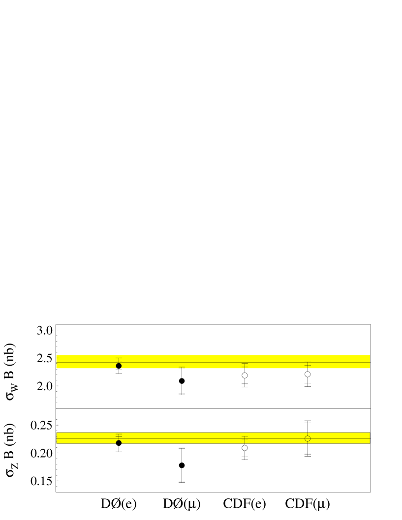
FIG. 15.: Measurements and predictions for $W\to l\nu$ and $Z\to ll$ cross sections. The results for this experiment are plotted as filled circles and those for the CDF experiment as open circles. The inner error bars represent the combined statistical and systematic uncertainties and the outer error bars include the uncertainty on integrated luminosity. The bands correspond to the range of predictions discussed in the text.

Channel	$W\rightarrow{e}\nu$	$Z\rightarrow{e^{+}e^{-}}$	$W\rightarrow\mu\nu$	$Z\rightarrow{\mu^{+}\mu^{-}}$
$N_{\rm obs}$	$10338$	$775$	$1665$	$77$
Total Bgd(%)	$5.7\pm 1.7$	$4.0\pm 1.4$	$22.1\pm 1.9$	$10.1\pm 3.7$
Acceptance(%)	$46.0\pm 0.6$	$36.3\pm 0.4$	$24.8\pm 0.7$	$6.5\pm 0.4$
$\epsilon_{\rm trig}\times\epsilon_{\rm sel}$(%)	$70.4\pm 1.7$	$73.6\pm 2.4$	$21.9\pm 2.2$	$52.7\pm 4.9$
$\rm\int{{\cal{L}}dt}\ ({\mbox{${\rm pb}^{-1}$}})$	$12.8\pm 0.7$	$12.8\pm 0.7$	$11.4\pm 0.6$	$11.4\pm 0.6$
$\sigma$B (nb)$\pm$(stat),	$2.36\pm 0.02$	$0.218\pm 0.008$	$2.09\pm 0.06$	$0.178\pm 0.022$
(sys),(lum)	$\pm 0.08\pm 0.13$	$\pm 0.008\pm 0.012$	$\pm 0.22\pm 0.11$	$\pm 0.021\pm 0.009$

TABLE IX.: Observed cross section multiplied by the leptonic branching fraction for $W$ and $Z$ boson production.

C Extraction of $B(W\to\ell\nu)$ and $\Gamma(W)$ from $R$

1 Phenomenological Considerations

The leptonic branching fraction and the total decay width of the $W$ boson can be extracted from the measured ratio of the cross sections multiplied by the branching fractions of the $W$ and $Z$ bosons into leptons. The ratio $R$ can be expressed as follows:

$$R\equiv\frac{\sigma_{W}\rm{B}(W\rightarrow\ell\nu)}{\sigma_{Z}\rm{B}(Z\rightarrow\ell\ell)}=\frac{\sigma_{W}}{\sigma_{Z}}\frac{1}{\rm{B}(Z\rightarrow\ell\ell)}\frac{\Gamma(W\rightarrow\ell\nu)}{\Gamma(W)}.$$ (34)

Using an experimental result for $R$, the known $\rm{B}(Z\rightarrow\ell\ell)$, and the prediction of ${\sigma_{W}}/{\sigma_{Z}}$, a value for the leptonic branching fraction of the $W$ boson follows:

$$\frac{\Gamma(W\rightarrow\ell\nu)}{\Gamma(W)}=\frac{\rm{B}(Z\rightarrow\ell\ell)}{\sigma_{W}/\sigma_{Z}}R=(0.01011\pm 0.00011)R.$$ (35)

Alternatively, using, in addition, a calculation of $\Gamma(W\rightarrow\ell\nu)$, the full width of the $W$ boson width $\Gamma(W)$ can be extracted:

$$\Gamma(W)=\frac{(\sigma_{W}/\sigma_{Z})\Gamma(W\rightarrow\ell\nu)}{\rm{B}(Z\rightarrow\ell\ell)}\frac{1}{R}.$$ (36)

The leptonic width of the $W$ boson can be written as:

$$\Gamma(W\rightarrow\ell\nu)=\frac{G_{F}M_{W}^{3}}{6\pi\sqrt{2}}(1+\delta^{\rm{SM}}).$$ (37)

The corrections $\delta^{\rm{SM}}$ have been calculated in the standard model by Rosner et al. [37]. Using $G_{F}=(1.16639\pm 0.00002)\times 10^{-5}$ GeV^-2, $M_{W}=80.23\pm 0.18$ GeV and $\delta^{\rm{SM}}=-0.35\%$ gives $\Gamma(W\rightarrow\ell\nu)=0.2252\pm 0.0015$ GeV, where the error is entirely due to the dependence on $M_{W}$.

In order to properly calculate the uncertainty on $\Gamma(W)$, it is necessary to take into account the correlation of errors on $\sigma_{W}/\sigma_{Z}$ and $\Gamma(W\rightarrow\ell\nu)$ due to dependence on $M_{W}$. The product of these factors is shown in Table X for a one standard deviation variation in $M_{W}$. Taking the side with the larger variation as the error, the variation in the product is 0.0009 GeV. The error on the product due to other sources is 0.0045 GeV; combining the errors in quadrature gives 0.0046 GeV. The product, using the nominal value of $\sigma_{W}/\sigma_{Z}=3.33$, is then

$$\frac{\sigma_{W}}{\sigma_{Z}}\Gamma(W\rightarrow\ell\nu)=0.7499\pm 0.0046\ {\rm GeV}.$$ (38)

Finally, using this value in the expression for $\Gamma(W)$ leads to

$$\Gamma(W)=(22.272\pm 0.137)\frac{1}{R}\rm{GeV}.$$ (39)

$M_{W}$	$\sigma_{W}/\sigma_{Z}$	$\Gamma(W\rightarrow\ell\nu)$	$(\sigma_{W}/\sigma_{Z})\Gamma(W\rightarrow\ell\nu)$
(GeV)		(GeV)	(GeV)
80.05	3.358	0.2237	0.7512 (+0.0008)
80.23	3.332	0.2252	0.7504
80.41	3.306	0.2267	0.7495 ($-0.0009$)

TABLE X.: Calculation of the product $(\sigma_{W}/\sigma_{Z})\Gamma(W\to\ell\nu)$ for a 1 $\sigma$ variation in $M_{W}$, using the pdf CTEQ2M.

2 Result of Measurements

The ratio of cross sections is given by:

$$R = \frac{N^{W}_{\rm{obs}}(1-f^{W}_{\rm{bgd}})}{N^{Z}_{\rm{obs}}(1-f^{Z}_{\rm{bgd}})}\frac{\varepsilon^{Z}}{\varepsilon^{W}}\frac{A^{Z}}{A^{W}}.$$

(The dependence on the luminosity is completely canceled in the ratio.) Our results for $e$ and $\mu$ channels are:

$$R_{e} = 10.82\pm 0.41(\mbox{stat})\pm 0.35(\mbox{syst}),$$

$$R_{\mu} = 11.8^{+1.8}_{-1.4}(\mbox{stat})\pm 1.1(\mbox{syst}),$$

and combined:

$$R_{e+\mu} = 10.90\pm 0.52(\mbox{stat$\oplus$syst}).$$

This is consistent with previous measurements shown in Fig. 16.

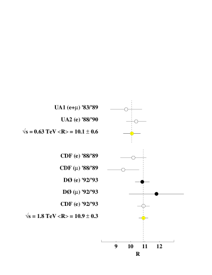
FIG. 16.: Measurements of the ratio of the $W\to l\nu$ and $Z\to ll$ cross sections multiplied by their respective branching fractions. The results are shown as a function of the years of the data run.

Using this result, we obtain the branching fraction

$$B(W\to l\nu)=(11.02\pm 0.52)\%.$$ (40)

Combining this measurement with the calculation of the partial width of the $W$ boson $\Gamma(W\rightarrow l\nu)$, we obtain

$$\Gamma(W)=2.044\pm 0.097\mbox{ GeV}.$$ (41)

This is in excellent agreement with the prediction of the standard model, $\Gamma(W)=2.077\pm 0.014$ GeV [37, 38], and with the world average value, $\Gamma(W)=2.06\pm 0.06$ GeV [11].

We can use our result to probe new possible decay modes of the $W$ boson, such as decays into supersymmetric charginos and neutralinos [39] or heavy quarks [40]. Since our experimentally measured central value of $\Gamma(W)/\Gamma(W\rightarrow l\nu)$ (the inverse of the branching fraction) falls below the mean predicted by the standard model, we use the asymmetric method to calculate limits on new decay modes [11]. From our data, we derive a 95% CL upper limit of 171 MeV on the width of unexpected decays of the $W$ boson. If a new heavy quark exists, the limit for its mass is $m_{q^{\prime}}>61$ GeV at the $95\%$ CL (see Fig. 17). Combining our result with other measurements [41] gives a weighted average of $\Gamma(W)=2.062\pm 0.060$ GeV, and a 95% CL upper limit of 111 MeV on unexpected decays.

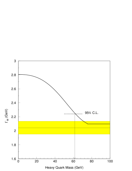
FIG. 17.: The width of the $W$ boson as a function of a new quark mass. Our measurement is shown as a one standard deviation band with the central value represented by the solid line. The darker curve represents the prediction of the standard model as a function of quark mass. The short dashed line indicates the upper limit at 95% CL on the width of the $W$ boson from our data.

Since the time that these results were first reported in a Letter [10], the knowledge of the mass of the $W$ boson has improved substantially. If we update the value used in Ref. [10] of $M_{W}=80.23\pm 0.18$ GeV to the current value of $M_{W}=80.39\pm 0.06$ GeV[42], the following results are obtained:

$$\sigma(W)\rm{B}(W\to e\nu)=2.35\pm 0.02\pm 0.08\pm 0.13\rm{nb},$$ (42)

$$B(W\to l\nu)=(11.03\pm 0.52)\%.$$ (43)

$$\Gamma(W)=2.054\pm 0.097\mbox{ GeV}$$ (44)

All other numbers reported change by much less than their uncertainties.

VIII Conclusions

DØ has measured the product of cross section and the lepton branching fraction for $W$ and $Z$ boson production in the electron and muon decay channels. We find

$$\sigma(W)\rm{B}(W\to e\nu) = 2.36\pm 0.02\pm 0.08\pm 0.13\rm{nb},$$

$$\sigma(W)\rm{B}(W\to\mu\nu) = 2.09\pm 0.06\pm 0.22\pm 0.11\rm{nb},$$

$$\sigma(Z)\rm{B}(Z\to ee) = 0.218\pm 0.008\pm 0.008\pm 0.012\rm{nb},$$

and

$$\sigma(Z)\rm{B}(Z\to\mu\mu) = 0.178\pm 0.022\pm 0.021\pm 0.009\rm{nb}.$$

Our values are in good agreement both with the ${\cal O}(\alpha_{s}^{2})$ QCD predictions using recent pdf sets, and with other measurements.

Including theoretical calculations for $\sigma_{W}/\sigma_{Z}$ and B$(Z\to ll)$, we measure

$$\rm{B}(W\to l\nu)=(11.02\pm 0.52)\%.$$ (45)

Adding the standard model prediction for $\Gamma(W\to l\nu)$, we find

$$\Gamma(W)=2.044\pm 0.097\mbox{ GeV}.$$ (46)

These results are in good agreement with the standard model, and allow us to set a limit on any new decay modes of the $W$ boson.

IX Acknowledgments

We thank the staffs at Fermilab and collaborating institutions for their contributions to this work, and acknowledge support from the Department of Energy and National Science Foundation (U.S.A.), Commissariat à L’Energie Atomique (France), Ministry for Science and Technology and Ministry for Atomic Energy (Russia), CAPES and CNPq (Brazil), Departments of Atomic Energy and Science and Education (India), Colciencias (Colombia), CONACyT (Mexico), Ministry of Education and KOSEF (Korea), and CONICET and UBACyT (Argentina).

REFERENCES

- [1] Visitor from Universidad San Francisco de Quito, Quito, Ecuador.
- [2] Visitor from IHEP, Beijing, China.
- [3] The UA1 Collaboration, C. Albajar et al., Phys. Lett. B 253, 503 (1991).
- [4] The UA2 Collaboration, J. Alitti et al., Phys. Lett. B 276, 365 (1992).
- [5] The CDF Collaboration, F. Abe et al., Phys Rev. Lett. 62, 1005 (1989).
- [6] The CDF Collaboration, F. Abe et al., Phys Rev. Lett. 64, 152 (1990).
- [7] The CDF Collaboration, F. Abe et al., Phys Rev. D 44, 29 (1991).
- [8] The CDF Collaboration, F. Abe et al., Phys Rev. Lett. 73, 220 (1994).
- [9] The CDF Collaboration, F. Abe et al., Phys Rev. Lett. 76, 3070 (1996).
- [10] The DØ Collaboration, S. Abachi et al., Phys. Rev. Lett. 75, 1456 (1995).
- [11] Particle Data Group, C. Caso et al., The European Physical Journal C3, 1 (1998).
- [12] The CDF Collaboration, F. Abe et al., Phys Rev. D 52, 2624 (1995).
- [13] The CDF Collaboration, F. Abe et al., Phys. Rev. Lett 74 341 (1995).
- [14] The DØ Collaboration, S. Abachi et al., Nucl. Instrum. Methods A338, 185 (1994).
- [15] The UA1 Collaboration, A. Astbury et al., UA1 Technical Proposal, CERN/SPSC/78-06, (1978); C. Cochet et al., Nucl. Instrum. Methods A243, 45, (1986); B. Aubert et al., Nucl. Instrum. Methods 176, 195, (1980); M. J. Corden et al., Nucl. Instrum. Methods A238, 273, (1985); M. Calvetti et al., IEEE Trans. Nucl. Sci. NS-30, 71, (1983).
- [16] The CDF Collaboration, F. Abe et al., Nucl. Instrum. Methods A271, 387 (1988).
-
[17]
J. Yang, Ph.D. thesis, (New York University, 1995)
(unpublished), http://www-d0.fnal.gov/jyang/all.ps; P. Grudberg,
Ph.D. thesis, (Univ. of California, Berkeley, 1997) (unpublished),
http://www-d0.fnal.gov/publications_talks/thesis/grudberg/thesis.ps - [18] C. Gerber, Ph.D. thesis, (Univ. of Buenos Aires, 1994) (unpublished), http://www-d0.fnal.gov/publications_talks/thesis/gerber/gerber_muxsec.ps
- [19] S. Youssef, Comp. Phys. Comm. 45, 423 (1987).
- [20] The DØ Collaboration, M. Narain, in The Fermilab Meeting Proceedings of Meeting of the Division of Particles and Fields of the American Physical Society, Batavia, Illinois, November 1992, edited by C.Albright, P.Kasper, R.Raja, and J.Yoh (World Scientific, Singapore, 1993).
- [21] The DØ Collaboration, B. Abbott et al., Phys. Rev. D 58, 12002 (1998).
- [22] The LEP collaborations, ALEPH, DELPHI, L3 and OPAL, Phys. Lett. B 276, 247 (1992)
-
[23]
The DØ Collaboration, J. A. Guida,
in Proceedings of the 4th International Conference
on Advanced Technology and Particle Physics,
Como, Italy, 1994 edited by E. Borchi, S. Majewski,
J. Huston, A. Penzo, P.G. Rancoita (North-Holland, 1995).
The DØ Collaboration, J. Kotcher, in Proceedings of the 1994 Beijing Calorimetry Symposium, IHEP - Chinese Academy of Sciences, Beijing, China, 1994, edited by He Sheng (Chen. Inst. High Energy Phys., 1995). - [24] The GEANT program and D0 modifications: R. Brun et al., GEANT User’s Guide v3.14, CERN Program Library (unpublished); F. Carminati et al., GEANT User’s Guide, CERN Program Library, 1991 (unpublished).
- [25] The DØ Collaboration, B. Abbott et al., Phys. Rev. Lett. 80, 5498 (1998).
- [26] The DØ Collaboration, S. Abachi et al., Phys. Rev. Lett. 74, 3548 (1998).
- [27] T. Sjöstrand, Computer Physics Commun. 82, 74(1994).
- [28] F. Paige, S. D. Protopopescu, ISAJET Monte Carlo, BNL Report No. BNL38034, 1986 (unpublished).
- [29] P. B. Arnold and R. P. Kauffman, Nucl. Phys. B 349, 381(1991); Peter B. Arnold, M. Hall Reno, Nucl. Phys. B 319, 37 (1989).
- [30] F. A. Berends and R. Kleiss, Zeit. Phys. C27, 365 (1985).
- [31] J. Bantly et al., Fermilab Report No. FERMILAB-TM-1930, 1995 (unpublished).
- [32] The CDF Collaboration, F. Abe et al., Phys Rev. Lett. 76, 3070 (1996).
- [33] The E-710 Collaboration, N. A. Amos et al., Phys Lett. B 243, 158 (1990).
- [34] R. Hamberg, W. L. van Neerven, and T. Matsuura, Nucl. Phys. B 359, 343 (1991).
- [35] H. L. Lai et al., Phys. Rev. D51, 4763 (1995).
- [36] W. L. van Neerven and E. B. Zijlstra, Nucl. Phys. B 382, 11 (1992).
- [37] J. L. Rosner, M. P. Worah, and T. Takeuchi, Phys. Rev. D49, 1363 (1994).
- [38] We used GeV from DØ Note 2115 and CDF Note 2552, 1994 (unpublished).
- [39] V. Barger et al., Phys. Rev. D28, 2912 (1983); M. Drees, C.S. Kim, and X. Tata, Phys. Rev. D37, 784 (1988).
- [40] T. Alvarez, A. Leites, and J. Terrón, Nucl. Phys. B 301, 1 (1988).
- [41] We recalculated for the other experiments [3, 4, 12] by using their published values along with the values of B and in this paper. For we used our value for CDF, and [4] for the UA1 and UA2 experiments at lower .
- [42] D. Karlen, to appear in the Proceedings of the 29th International Conference on High Energy Physics, Vancouver, Canada, 1998.