Abstract

Searches for pair-produced charginos and neutralinos with $R$-parity violating decays have been performed using a data sample corresponding to an integrated luminosity of 56 pb^-1 collected with the OPAL detector at LEP at a centre-of-mass energy of $\sqrt{s}=$ 183 GeV. An important consequence of $R$-parity violation is that the lightest supersymmetric particle becomes unstable. The searches have been performed under the assumptions that the lightest supersymmetric particle promptly decays and that only one $R$-parity violating coupling is dominant for each of the decay modes considered. Such processes would yield multiple leptons, jets plus leptons, or multiple jets with or without significant missing energy in the final state. No excess of such events above Standard Model backgrounds has been observed. Limits are presented on the production cross-sections of gauginos in $R$-parity violating scenarios. Limits are also presented in the framework of the Minimal Supersymmetric Standard Model.

The OPAL Collaboration

G. Abbiendi², K. Ackerstaff⁸, G. Alexander²³, J. Allison¹⁶, N. Altekamp⁵, K.J. Anderson⁹, S. Anderson¹², S. Arcelli¹⁷, S. Asai²⁴, S.F. Ashby¹, D. Axen²⁹, G. Azuelos^18,a, A.H. Ball¹⁷, E. Barberio⁸, R.J. Barlow¹⁶, R. Bartoldus³, J.R. Batley⁵, S. Baumann³, J. Bechtluft¹⁴, T. Behnke²⁷, K.W. Bell²⁰, G. Bella²³, A. Bellerive⁹, S. Bentvelsen⁸, S. Bethke¹⁴, S. Betts¹⁵, O. Biebel¹⁴, A. Biguzzi⁵, S.D. Bird¹⁶, V. Blobel²⁷, I.J. Bloodworth¹, P. Bock¹¹, J. Böhme¹⁴, D. Bonacorsi², M. Boutemeur³⁴, S. Braibant⁸, P. Bright-Thomas¹, L. Brigliadori², R.M. Brown²⁰, H.J. Burckhart⁸, P. Capiluppi², R.K. Carnegie⁶, A.A. Carter¹³, J.R. Carter⁵, C.Y. Chang¹⁷, D.G. Charlton^1,b, D. Chrisman⁴, C. Ciocca², P.E.L. Clarke¹⁵, E. Clay¹⁵, I. Cohen²³, J.E. Conboy¹⁵, O.C. Cooke⁸, C. Couyoumtzelis¹³, R.L. Coxe⁹, M. Cuffiani², S. Dado²², G.M. Dallavalle², R. Davis³⁰, S. De Jong¹², A. de Roeck⁸, P. Dervan¹⁵, K. Desch⁸, B. Dienes^33,d, M.S. Dixit⁷, J. Dubbert³⁴, E. Duchovni²⁶, G. Duckeck³⁴, I.P. Duerdoth¹⁶, D. Eatough¹⁶, P.G. Estabrooks⁶, E. Etzion²³, F. Fabbri², M. Fanti², A.A. Faust³⁰, F. Fiedler²⁷, M. Fierro², I. Fleck⁸, R. Folman²⁶, A. Fürtjes⁸, D.I. Futyan¹⁶, P. Gagnon⁷, J.W. Gary⁴, J. Gascon¹⁸, S.M. Gascon-Shotkin¹⁷, G. Gaycken²⁷, C. Geich-Gimbel³, G. Giacomelli², P. Giacomelli², V. Gibson⁵, W.R. Gibson¹³, D.M. Gingrich^30,a, D. Glenzinski⁹, J. Goldberg²², W. Gorn⁴, C. Grandi², K. Graham²⁸, E. Gross²⁶, J. Grunhaus²³, M. Gruwé²⁷, G.G. Hanson¹², M. Hansroul⁸, M. Hapke¹³, K. Harder²⁷, A. Harel²², C.K. Hargrove⁷, C. Hartmann³, M. Hauschild⁸, C.M. Hawkes¹, R. Hawkings²⁷, R.J. Hemingway⁶, M. Herndon¹⁷, G. Herten¹⁰, R.D. Heuer²⁷, M.D. Hildreth⁸, J.C. Hill⁵, P.R. Hobson²⁵, M. Hoch¹⁸, A. Hocker⁹, K. Hoffman⁸, R.J. Homer¹, A.K. Honma^28,a, D. Horváth^32,c, K.R. Hossain³⁰, R. Howard²⁹, P. Hüntemeyer²⁷, P. Igo-Kemenes¹¹, D.C. Imrie²⁵, K. Ishii²⁴, F.R. Jacob²⁰, A. Jawahery¹⁷, H. Jeremie¹⁸, M. Jimack¹, C.R. Jones⁵, P. Jovanovic¹, T.R. Junk⁶, D. Karlen⁶, V. Kartvelishvili¹⁶, K. Kawagoe²⁴, T. Kawamoto²⁴, P.I. Kayal³⁰, R.K. Keeler²⁸, R.G. Kellogg¹⁷, B.W. Kennedy²⁰, D.H. Kim¹⁹, A. Klier²⁶, S. Kluth⁸, T. Kobayashi²⁴, M. Kobel^3,e, D.S. Koetke⁶, T.P. Kokott³, M. Kolrep¹⁰, S. Komamiya²⁴, R.V. Kowalewski²⁸, T. Kress⁴, P. Krieger⁶, J. von Krogh¹¹, T. Kuhl³, P. Kyberd¹³, G.D. Lafferty¹⁶, H. Landsman²², D. Lanske¹⁴, J. Lauber¹⁵, S.R. Lautenschlager³¹, I. Lawson²⁸, J.G. Layter⁴, D. Lazic²², A.M. Lee³¹, D. Lellouch²⁶, J. Letts¹², L. Levinson²⁶, R. Liebisch¹¹, B. List⁸, C. Littlewood⁵, A.W. Lloyd¹, S.L. Lloyd¹³, F.K. Loebinger¹⁶, G.D. Long²⁸, M.J. Losty⁷, J. Ludwig¹⁰, D. Liu¹², A. Macchiolo², A. Macpherson³⁰, W. Mader³, M. Mannelli⁸, S. Marcellini², C. Markopoulos¹³, A.J. Martin¹³, J.P. Martin¹⁸, G. Martinez¹⁷, T. Mashimo²⁴, P. Mättig²⁶, W.J. McDonald³⁰, J. McKenna²⁹, E.A. Mckigney¹⁵, T.J. McMahon¹, R.A. McPherson²⁸, F. Meijers⁸, S. Menke³, F.S. Merritt⁹, H. Mes⁷, J. Meyer²⁷, A. Michelini², S. Mihara²⁴, G. Mikenberg²⁶, D.J. Miller¹⁵, R. Mir²⁶, W. Mohr¹⁰, A. Montanari², T. Mori²⁴, K. Nagai⁸, I. Nakamura²⁴, H.A. Neal¹², B. Nellen³, R. Nisius⁸, S.W. O’Neale¹, F.G. Oakham⁷, F. Odorici², H.O. Ogren¹², M.J. Oreglia⁹, S. Orito²⁴, J. Pálinkás^33,d, G. Pásztor³², J.R. Pater¹⁶, G.N. Patrick²⁰, J. Patt¹⁰, R. Perez-Ochoa⁸, S. Petzold²⁷, P. Pfeifenschneider¹⁴, J.E. Pilcher⁹, J. Pinfold³⁰, D.E. Plane⁸, P. Poffenberger²⁸, J. Polok⁸, M. Przybycień⁸, C. Rembser⁸, H. Rick⁸, S. Robertson²⁸, S.A. Robins²², N. Rodning³⁰, J.M. Roney²⁸, K. Roscoe¹⁶, A.M. Rossi², Y. Rozen²², K. Runge¹⁰, O. Runolfsson⁸, D.R. Rust¹², K. Sachs¹⁰, T. Saeki²⁴, O. Sahr³⁴, W.M. Sang²⁵, E.K.G. Sarkisyan²³, C. Sbarra²⁹, A.D. Schaile³⁴, O. Schaile³⁴, F. Scharf³, P. Scharff-Hansen⁸, J. Schieck¹¹, B. Schmitt⁸, S. Schmitt¹¹, A. Schöning⁸, M. Schröder⁸, M. Schumacher³, C. Schwick⁸, W.G. Scott²⁰, R. Seuster¹⁴, T.G. Shears⁸, B.C. Shen⁴, C.H. Shepherd-Themistocleous⁸, P. Sherwood¹⁵, G.P. Siroli², A. Sittler²⁷, A. Skuja¹⁷, A.M. Smith⁸, G.A. Snow¹⁷, R. Sobie²⁸, S. Söldner-Rembold¹⁰, S. Spagnolo²⁰, M. Sproston²⁰, A. Stahl³, K. Stephens¹⁶, J. Steuerer²⁷, K. Stoll¹⁰, D. Strom¹⁹, R. Ströhmer³⁴, B. Surrow⁸, S.D. Talbot¹, S. Tanaka²⁴, P. Taras¹⁸, S. Tarem²², R. Teuscher⁸, M. Thiergen¹⁰, J. Thomas¹⁵, M.A. Thomson⁸, E. von Törne³, E. Torrence⁸, S. Towers⁶, I. Trigger¹⁸, Z. Trócsányi³³, E. Tsur²³, A.S. Turcot⁹, M.F. Turner-Watson¹, I. Ueda²⁴, R. Van Kooten¹², P. Vannerem¹⁰, M. Verzocchi¹⁰, H. Voss³, F. Wäckerle¹⁰, A. Wagner²⁷, C.P. Ward⁵, D.R. Ward⁵, P.M. Watkins¹, A.T. Watson¹, N.K. Watson¹, P.S. Wells⁸, N. Wermes³, J.S. White⁶, G.W. Wilson¹⁶, J.A. Wilson¹, T.R. Wyatt¹⁶, S. Yamashita²⁴, G. Yekutieli²⁶, V. Zacek¹⁸, D. Zer-Zion⁸

¹School of Physics and Astronomy, University of Birmingham, Birmingham B15 2TT, UK
²Dipartimento di Fisica dell’ Università di Bologna and INFN, I-40126 Bologna, Italy
³Physikalisches Institut, Universität Bonn, D-53115 Bonn, Germany
⁴Department of Physics, University of California, Riverside CA 92521, USA
⁵Cavendish Laboratory, Cambridge CB3 0HE, UK
⁶Ottawa-Carleton Institute for Physics, Department of Physics, Carleton University, Ottawa, Ontario K1S 5B6, Canada
⁷Centre for Research in Particle Physics, Carleton University, Ottawa, Ontario K1S 5B6, Canada
⁸CERN, European Organisation for Particle Physics, CH-1211 Geneva 23, Switzerland
⁹Enrico Fermi Institute and Department of Physics, University of Chicago, Chicago IL 60637, USA
¹⁰Fakultät für Physik, Albert Ludwigs Universität, D-79104 Freiburg, Germany
¹¹Physikalisches Institut, Universität Heidelberg, D-69120 Heidelberg, Germany
¹²Indiana University, Department of Physics, Swain Hall West 117, Bloomington IN 47405, USA
¹³Queen Mary and Westfield College, University of London, London E1 4NS, UK
¹⁴Technische Hochschule Aachen, III Physikalisches Institut, Sommerfeldstrasse 26-28, D-52056 Aachen, Germany
¹⁵University College London, London WC1E 6BT, UK
¹⁶Department of Physics, Schuster Laboratory, The University, Manchester M13 9PL, UK
¹⁷Department of Physics, University of Maryland, College Park, MD 20742, USA
¹⁸Laboratoire de Physique Nucléaire, Université de Montréal, Montréal, Quebec H3C 3J7, Canada
¹⁹University of Oregon, Department of Physics, Eugene OR 97403, USA
²⁰CLRC Rutherford Appleton Laboratory, Chilton, Didcot, Oxfordshire OX11 0QX, UK
²²Department of Physics, Technion-Israel Institute of Technology, Haifa 32000, Israel
²³Department of Physics and Astronomy, Tel Aviv University, Tel Aviv 69978, Israel
²⁴International Centre for Elementary Particle Physics and Department of Physics, University of Tokyo, Tokyo 113-0033, and Kobe University, Kobe 657-8501, Japan
²⁵Institute of Physical and Environmental Sciences, Brunel University, Uxbridge, Middlesex UB8 3PH, UK
²⁶Particle Physics Department, Weizmann Institute of Science, Rehovot 76100, Israel
²⁷Universität Hamburg/DESY, II Institut für Experimental Physik, Notkestrasse 85, D-22607 Hamburg, Germany
²⁸University of Victoria, Department of Physics, P O Box 3055, Victoria BC V8W 3P6, Canada
²⁹University of British Columbia, Department of Physics, Vancouver BC V6T 1Z1, Canada
³⁰University of Alberta, Department of Physics, Edmonton AB T6G 2J1, Canada
³¹Duke University, Dept of Physics, Durham, NC 27708-0305, USA
³²Research Institute for Particle and Nuclear Physics, H-1525 Budapest, P O Box 49, Hungary
³³Institute of Nuclear Research, H-4001 Debrecen, P O Box 51, Hungary
³⁴Ludwigs-Maximilians-Universität München, Sektion Physik, Am Coulombwall 1, D-85748 Garching, Germany

^a and at TRIUMF, Vancouver, Canada V6T 2A3
^b and Royal Society University Research Fellow
^c and Institute of Nuclear Research, Debrecen, Hungary
^d and Department of Experimental Physics, Lajos Kossuth University, Debrecen, Hungary
^e on leave of absence from the University of Freiburg

1 Introduction

In the general Lagrangian of the Minimal Supersymmetric extension of the Standard Model (MSSM) [1], the terms violating lepton ($L$) and baryon ($B$) numbers can be written as :

$${\cal L}_{RPV}=\lambda_{ijk}L_{i}L_{j}{\overline{E}}_{k}+\lambda^{{}^{\prime}}_{ijk}L_{i}Q_{j}{\overline{D}}_{k}+\lambda^{{}^{\prime\prime}}_{ijk}{\overline{U}}_{i}{\overline{D}}_{j}{\overline{D}}_{k},$$

where $i,j,k$ are the generation indices of the superfields $L,Q,E,D$ and $U$. $L$ and $Q$ are lepton and quark left-handed doublets, respectively. $\overline{E}$, $\overline{D}$ and $\overline{U}$ are right-handed singlet charge-conjugate superfields for the charged leptons and down- and up-type quarks, respectively. Yukawa couplings are denoted by $\lambda$, $\lambda^{{}^{\prime}}$, and $\lambda^{{}^{\prime\prime}}$. The first term in ${\cal L}_{RPV}$ is anti-symmetric in $i$ and $j$, the third one anti-symmetric in $j$ and $k$, and $i<j$ for $\lambda$ and $j<k$ for $\lambda^{{}^{\prime\prime}}$. This makes a total of $9+27+9=45$ parameters in addition to those of the $R$-parity conserving MSSM.

For a large range of values for $\lambda$, $\lambda^{{}^{\prime}}$, and $\lambda^{{}^{\prime\prime}}$  these terms lead to effects like a short proton lifetime, in contradiction with present experimental results. To avoid such effects, a new multiplicative quantum number, called $R$-parity, and defined as $R_{p}=(-1)^{2S+3B+L}$ is introduced, where $S$ is the spin, and postulated to be conserved. This is equivalent to setting all couplings $\lambda$, $\lambda^{{}^{\prime}}$, and $\lambda^{{}^{\prime\prime}}$ to zero. $R$-parity discriminates between ordinary and supersymmetric particles: $R_{p}$ = +1 for the Standard Model particles and $R_{p}$ = $-1$ for their supersymmetric partners. $R$-parity conservation implies that supersymmetric particles are always pair-produced and always decay through cascade decays to ordinary particles plus the lightest supersymmetric particle (LSP). The LSP has to be stable and is a cold dark matter candidate, if neutral.

However there is no a priori law that requires the conservation of $R$-parity. Strong experimental constraints only exist on the product of two $\lambda$-couplings, and therefore ${\cal L}_{RPV}$ is not excluded by experimental results under the assumption that only one of the $\lambda$-couplings is significantly different from zero. For example the non-observation of proton decay results in the limits $\lambda_{11k}^{{}^{\prime}}\cdot\lambda_{11k}^{{}^{\prime\prime}}\leq 10^{-22}$ [2] for $k=2,3$. A more general limit gives $\lambda_{ijk}^{{}^{\prime}}\cdot\lambda_{lmn}^{{}^{\prime\prime}}\leq 10^{-10}$ [3]. Limits on individual couplings are calculated e.g. from searches for neutrinoless double beta decay or from tests of lepton universality in pion or tau decays, and are of order $10^{-2}$ for most couplings. A complete listing of all existing limits is given in [4].

The main consequence of $R$-parity violation is an unstable LSP, yielding different experimental signatures compared to $R$-parity conservation. Also, in this case, the $\tilde{\chi}^{0}_{1}$ is not a cold dark matter candidate, and mass limits for $\tilde{\chi}^{0}_{1}$ cannot be interpreted as such. Results for decays via the coupling $\lambda$ have been presented by ALEPH [5]. With $R$-parity violation the production of single sparticles becomes possible and limits from OPAL are given in [6].

The model used in this paper is a constrained Minimal Supersymmetric Model (CMSSM) [7, 8, 9, 10]. It has only five free parameters not counting the additional 45 Yukawa couplings $\lambda$, $\lambda^{{}^{\prime}}$, and $\lambda^{{}^{\prime\prime}}$. A common mass is assumed for the gauginos, ($m_{1/2}$), and for the sfermions, ($m_{0}$), at the GUT scale. The other free parameters are $\mu$, the mixing parameter of the two Higgs field doublets, $\tan\beta$, the ratio of the vacuum expectation values of the two Higgs doublets, and $A$, a tri-linear coupling. By also assuming gauge unification at the GUT scale, the masses at the electroweak scale of the U(1)_Y gaugino, ($M_{1}$), and of the soft SUSY breaking SU(2)_L gaugino, ($M_{2}$), are related by $M_{1}=\frac{5}{3}\tan^{2}\theta_{\mathrm{W}}M_{2}$ with $\theta_{\mathrm{W}}$ the weak mixing angle and $M_{1}=0.42m_{1/2}$.

In this paper we present searches, assuming $R$-parity violation, for the pair production of charginos ($\tilde{\chi}^{\pm}_{1}$) and neutralinos ($\tilde{\chi}^{0}_{1}$) with the OPAL detector at a centre-of-mass energy of 183 GeV at the LEP e⁺e^- collider at CERN, using an integrated luminosity of $\sim$ 56 pb^-1. Decays via $\lambda$, $\lambda^{{}^{\prime}}$, and $\lambda^{{}^{\prime\prime}}$ couplings are searched for. We further assume a prompt decay of all SUSY particles, and design our searches to be sensitive only to particles decaying close to the interaction vertex. This corresponds to a sensitivity for values of $\lambda$, $\lambda^{{}^{\prime}}$, and $\lambda^{{}^{\prime\prime}}$ greater than $\sim 10^{-5}$. The assumption of heavy sfermion masses is made in addition.

2 Gaugino Production and Decay

In electron-positron collisions, charginos and neutralinos can be pair-produced through $s$-channel processes involving ${\mathrm{Z}}^{0}$ or $\gamma$ exchange. They can also be produced through $t$-channel exchange of an electron-sneutrino, ($\tilde{\nu}_{e}$), or a selectron, ($\tilde{\mathrm{e}}$). The chargino (neutralino) pair production cross-section is reduced (enhanced) due to interference between the $s$- and $t$-channels.

2.1 Decay Modes

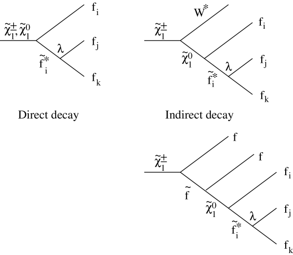
We distinguish direct and indirect decays, as shown in Figure 1.

In the direct mode, the gaugino decays into a fermion and a virtual sfermion which, in turn, decays via the $R$-parity violating Lagrangian. In the indirect mode,the $R$-parity violating transition occurs at a later stage in the decay sequence. In this paper both the direct decays of the $\tilde{\chi}^{\pm}_{1}$ and $\tilde{\chi}^{0}_{1}$ and the indirect decays of the $\tilde{\chi}^{\pm}_{1}$, shown in Figure 1, are considered. Throughout, we assume that only one of the couplings $\lambda$, $\lambda^{{}^{\prime}}$, or $\lambda^{{}^{\prime\prime}}$ is different from zero.

2.1.1 Direct Decays

The direct decay of a gaugino produces three fermions and the pair-production of gauginos results in 6-fermion final states. The type (lepton or quark) of the fermions is determined by the couplings $\lambda$, $\lambda^{{}^{\prime}}$, and $\lambda^{{}^{\prime\prime}}$ while the flavour is determined by the indices of the couplings.

For non-vanishing $\lambda$, the decay of a $\tilde{\chi}^{0}_{1}$ via the $\lambda$${}_{ijk}L_{i}L_{j}{\overline{E}}_{k}$ operator results in the following final states:

$\tilde{\chi}^{0}_{1}\rightarrow\ell^{-}_{i}\nu_{j}\ell^{+}_{k}$,  $\tilde{\chi}^{0}_{1}\rightarrow\ell^{+}_{i}\overline{\nu}_{j}\ell^{-}_{k}$,  $\tilde{\chi}^{0}_{1}\rightarrow\nu_{i}\ell^{-}_{j}\ell^{+}_{k}$,  $\tilde{\chi}^{0}_{1}\rightarrow\overline{\nu}_{i}\ell^{+}_{j}\ell^{-}_{k}$

Figure 1: Direct and indirect decays.

In each case, one of the leptons is a neutrino, and the other two have opposite electric charge. The flavours of the leptons are not correlated. This results in final states with four charged leptons and missing energy.

For the decay of a $\tilde{\chi}^{\pm}_{1}$ via the $\lambda$${}_{ijk}L_{i}L_{j}{\overline{E}}_{k}$ operator the final states are:

$\tilde{\chi}^{+}_{1}\rightarrow\nu_{i}\nu_{j}\ell^{+}_{k}$,  $\tilde{\chi}^{+}_{1}\rightarrow\ell^{+}_{i}\ell^{+}_{j}\ell^{-}_{k}$,  $\tilde{\chi}^{+}_{1}\rightarrow\ell^{+}_{i}\overline{\nu}_{j}\nu_{k}$,  $\tilde{\chi}^{+}_{1}\rightarrow\overline{\nu}_{i}\ell^{+}_{j}\nu_{k}$

with either one charged lepton plus two neutrinos or three charged leptons.

The final states with one charged lepton with index $i$ or $j$ are strongly suppressed because they involve the decay of the $\tilde{\chi}^{\pm}_{1}$ into a neutrino from the left handed lepton doublet field and a slepton from the right handed singlet field. These final states, which can occur via mixing of the left– and right–handed states into the mass eigenstates, are neglected within this paper. Consequently, the final state consists of two leptons of the same flavour and missing energy, four charged leptons with missing energy or six charged leptons and no missing energy.

For non-vanishing $\lambda^{{}^{\prime}}$, both the $\tilde{\chi}^{0}_{1}\$ and the $\tilde{\chi}^{\pm}_{1}\$ decay into a lepton and two quarks through the $\lambda^{{}^{\prime}}_{ijk}L_{i}Q_{j}{\overline{D}}_{k}$ operator. The possible decays are respectively:

$\tilde{\chi}^{0}_{1}\rightarrow\ell^{-}_{i}u_{j}\overline{d}_{k}$,  $\tilde{\chi}^{0}_{1}\rightarrow\ell^{+}_{i}\overline{u}_{j}d_{k}$,  $\tilde{\chi}^{0}_{1}\rightarrow\nu_{i}d_{j}\overline{d}_{k}$,  $\tilde{\chi}^{0}_{1}\rightarrow\overline{\nu}_{i}\overline{d}_{j}d_{k}$

and

$\tilde{\chi}^{+}_{1}\rightarrow\nu_{i}u_{j}\overline{d}_{k}$,  $\tilde{\chi}^{+}_{1}\rightarrow\overline{\nu}_{i}\overline{d}_{j}u_{k}$  $\tilde{\chi}^{+}_{1}\rightarrow\ell^{+}_{i}\overline{d}_{j}d_{k}$,  $\tilde{\chi}^{+}_{1}\rightarrow\ell^{+}_{i}\overline{u}_{j}u_{k}$

These decays result in final states with four jets and either missing energy, or one charged lepton with missing energy, or two charged leptons.

For non-vanishing $\lambda^{{}^{\prime\prime}}$, both the $\tilde{\chi}^{0}_{1}\$ and the $\tilde{\chi}^{\pm}_{1}\$ decay into three quarks through the $\lambda^{{}^{\prime\prime}}_{ijk}{\overline{U}}_{i}{\overline{D}}_{j}{\overline{D}}_{k}$ operator. The possible decays are:

$\tilde{\chi}^{0}_{1}\rightarrow\overline{u}_{i}\overline{d}_{j}\overline{d}_{k}$,  $\tilde{\chi}^{0}_{1}\rightarrow u_{i}d_{j}d_{k}$

and

$\tilde{\chi}^{+}_{1}\rightarrow\overline{d}_{i}\overline{d}_{j}\overline{d}_{k}$,  $\tilde{\chi}^{+}_{1}\rightarrow u_{i}u_{j}d_{k}$,  $\tilde{\chi}^{+}_{1}\rightarrow u_{i}d_{j}u_{k}$

and the final states consist of six jets in each case (with no missing energy). Table 1 lists the decay modes for the direct decays of a chargino pair and a neutralino pair.

2.1.2 Indirect Decays

In the indirect decay mode, the chargino decays via the $R$-parity conserving couplings to a neutralino and Standard Model particles, and the neutralino decays via the $R$-parity violating Lagrangian.

The $\tilde{\chi}^{\pm}_{1}$ decays into five fermions with three arising from the decay of the $\tilde{\chi}^{0}_{1}$ and two from the decay of a W^(∗) boson. The decay products of the $\tilde{\chi}^{0}_{1}$ depend on the coupling $\lambda$, $\lambda^{{}^{\prime}}$, or $\lambda^{{}^{\prime\prime}}$ and are the same as in the direct decay of the $\tilde{\chi}^{0}_{1}$. The final states therefore consist of 10 fermions, varying between six leptons and missing energy and ten jets.

Besides decaying via $\tilde{\chi}^{\pm}_{1}\rightarrow\tilde{\chi}^{0}_{1}$ W^(∗), the chargino can also decay via $\tilde{\chi}^{\pm}_{1}\rightarrow\tilde{\mathrm{f}}$f. In this case the subsequent decay of the sfermion $\tilde{\mathrm{f}}\rightarrow\tilde{\chi}^{0}_{1}\mathrm{f}\rightarrow$ (fff) f leads to chargino decays into five fermions, and the final state is a subset of the final states from the indirect decays already considered.

Of the cascade decays involving a $\tilde{\chi}^{0}_{2}$ we only consider the decay $\tilde{\chi}^{0}_{2}\rightarrow\tilde{\chi}^{0}_{1}\gamma$. Table 2 lists all final states for the indirect decay of a chargino pair via a W^(∗) boson. For decays via a sfermion, the final states are a subset of these states.

2.1.3 Mixed Decays

Whether a sparticle decays via the direct or the indirect mode depends on the precise value of the MSSM parameters and the size of the $\lambda$–coupling. When the decay width for direct and indirect decay modes are similar, the mixed mode occurs with one sparticle decaying directly and the other indirectly. We have not investigated these final states, except for decays via $\lambda^{{}^{\prime\prime}}$; but they are taken into account for all $\lambda$-couplings when interpreting the search results in Chapter 7.

	$\tilde{\chi}^{+}_{1}\tilde{\chi}^{-}_{1}\rightarrow$		$\tilde{\chi}^{0}_{1}\tilde{\chi}^{0}_{1}\rightarrow$
$\lambda$ coupling	$\ell_{i}\ell_{j}\ell_{k}$	$\ell_{i}\ell_{j}\ell_{k}$	$\nu\ell^{+}\ell^{-}$	$\nu\ell^{+}\ell^{-}$
	$\ell_{i}\ell_{j}\ell_{k}$	$\nu\nu\ell_{k}$
	$\nu\nu\ell_{k}$	$\nu\nu\ell_{k}$
$\lambda^{{}^{\prime}}$ coupling	$\ell_{i}qq$	$\ell_{i}qq$	$\ell_{i}qq$	$\ell_{i}qq$
	$\ell_{i}qq$	$\nu qq$	$\ell_{i}qq$	$\nu qq$
	$\nu qq$	$\nu qq$	$\nu qq$	$\nu qq$
$\lambda^{{}^{\prime\prime}}$ coupling	$qqq$	$qqq$	$qqq$	$qqq$

Table 1: Final states resulting from the direct decay modes of a $\tilde{\chi}^{\pm}_{1}$ and $\tilde{\chi}^{0}_{1}$ pair. The final states consist of all 6 fermions listed in any one line. Any fermion symbol ( $\ell,\nu,q$ ) means particle or anti-particle with arbitrary flavour, obeying the conditions from the Lagrangian. $\ell_{i(j,k)}$ is a lepton with flavour $i(j,k)\quad(i=1,2,3)$. The indices $i,j$, and $k$ correspond to the indices of the Yukawa couplings $\lambda$ and $\lambda^{{}^{\prime}}$.

$\tilde{\chi}^{+}_{1}\tilde{\chi}^{-}_{1}\rightarrow$	W(∗)	W(∗)	$\tilde{\chi}^{0}_{1}$	$\tilde{\chi}^{0}_{1}$
$\lambda$ coupling	$\ell^{+}\nu$	$\ell^{-}\nu$	$\nu\ell^{+}\ell^{-}$	$\nu\ell^{+}\ell^{-}$
	$\ell\nu$	$qq$	$\nu\ell^{+}\ell^{-}$	$\nu\ell^{+}\ell^{-}$
	$qq$	$qq$	$\nu\ell^{+}\ell^{-}$	$\nu\ell^{+}\ell^{-}$
$\lambda^{{}^{\prime}}$ coupling	$\ell^{+}\nu$	$\ell^{-}\nu$	$\ell_{i}qq$	$\ell_{i}qq$
	$\ell^{+}\nu$	$\ell^{-}\nu$	$\ell_{i}qq$	$\nu_{i}qq$
	$\ell^{+}\nu$	$\ell^{-}\nu$	$\nu_{i}qq$	$\nu_{i}qq$
	$\ell\nu$	$qq$	$\ell_{i}qq$	$\ell_{i}qq$
	$\ell\nu$	$qq$	$\ell_{i}qq$	$\nu_{i}qq$
	$\ell\nu$	$qq$	$\nu_{i}qq$	$\nu_{i}qq$
	$qq$	$qq$	$\ell_{i}qq$	$\ell_{i}qq$
	$qq$	$qq$	$\ell_{i}qq$	$\nu_{i}qq$
	$qq$	$qq$	$\nu_{i}qq$	$\nu_{i}qq$
$\lambda^{{}^{\prime\prime}}$ coupling	$\ell^{+}\nu$	$\ell^{-}\nu$	$qqq$	$qqq$
	$\ell\nu$	$qq$	$qqq$	$qqq$
	$qq$	$qq$	$qqq$	$qqq$

Table 2: Final states resulting from the indirect decay modes of a $\tilde{\chi}^{\pm}_{1}$ pair, including only decays directly to the $\tilde{\chi}^{0}_{1}$. Cascade decays via other sparticles are not included. The final states consist of all 10 fermions listed in any one line. Any fermion symbol ( $\ell,\nu,q$ ) means particle or anti-particle with any flavour being allowed. $\ell_{i},\nu_{i}$ is a lepton with flavour $i(i=1,2,3)$, where $i$ is determined by the first index in the $\lambda^{{}^{\prime}}$ coupling. The final states listed here are for a decay via a W^(∗) boson.

2.2 Decay Widths

The decay width of gauginos is governed by their field contents and the size of the $\lambda$-coupling. The full matrix elements needed to calculate the decay widths for $\tilde{\chi}^{\pm}_{1}$ and $\tilde{\chi}^{0}_{1}$ are given in [12] and [13], respectively.

For a pure photino-like $\tilde{\chi}^{0}_{1}$, the decay width for the $\lambda$${}_{ijk}L_{i}L_{j}{\overline{E}}_{k}$ operator is given by [14]:

$$\Gamma=\lambda^{2}\frac{\alpha}{128\pi^{2}}\frac{(m_{\tilde{\chi}^{0}_{1}})^{5}}{(m_{\tilde{f}})^{4}},$$

where $\alpha$ is the fine-structure constant and $m_{\tilde{f}}$ is the mass of the virtual sfermion in the decay. For the $\lambda^{{}^{\prime}}$${}_{ijk}L_{i}Q_{j}{\overline{D}}_{k}$ operator the decay width $\Gamma$ has to be multiplied by $3\cdot e_{q}^{2}$, with $e_{q}$ the charge of the virtual squark.

Assuming a decay length less than a few millimeters, and a sfermion mass $m_{\tilde{f}}$ of 100 GeV, gives a sensitivity for $\lambda$ greater than ${\cal{O}}(10^{-5})$ for $\tilde{\chi}^{0}_{1}$ masses accessible at LEP2, much lower than the strongest existing limits, of $\sim 0.0003$ [15], on any coupling $\lambda$ or $\lambda^{{}^{\prime}}$.

For very long lifetimes, the LSP decays outside the detector, and the event topology is exactly the same as in the $R_{p}$ conserving case. This case is covered by gaugino searches assuming $R$-parity conservation [16].

3 Event Simulation

Signal and background events have been generated, passed through the full detector simulation [17] and the same analysis chain as the real data.

3.1 Signal

The simulation of the signal events has been done with the Monte Carlo program SUSYGEN [18]. For the direct decays, events have been produced for the mass values of 45, 70 and 90 GeV with a $m_{0}$ of 1 TeV and at a mass of 70 GeV for a $m_{0}$ of 48.4 GeV for the $\tilde{\chi}^{\pm}_{1}$. For the $\tilde{\chi}^{0}_{1}$ in addition to the four mass points mentioned above also a mass value of 30 GeV has been generated, as there exists no direct mass limit from the LEP1 data. The mass values for the $\tilde{\chi}^{\pm}_{1}$ have been chosen to cover the range between the masses already excluded from the LEP1 data and the kinematic limit of the 183 GeV centre-of-mass energy.

For the indirect decay of the charginos, $\Delta m=m_{\tilde{\chi}^{\pm}_{1}}-m_{\tilde{\chi}^{0}_{1}}=m_{\tilde{\chi}^{\pm}_{1}}/2$ and $m_{0}$ = 1 TeV have been chosen for $\tilde{\chi}^{\pm}_{1}$ mass values of 45, 70 and 90 GeV. Additional events have been generated at $m_{\tilde{\chi}^{\pm}_{1}}$ = 70 GeV and $\Delta m=m_{\tilde{\chi}^{\pm}_{1}}/2$ with $m_{0}$ = 48.4 GeV, leading to an enhanced t-channel contribution, and at $m_{\tilde{\chi}^{\pm}_{1}}$ = 90 GeV for $\Delta m=$ 5 GeV to account for changes in the event topologies from the model parameters. The values of $\Delta m$ have been chosen to cover a large range for a limited number of Monte Carlo samples. Differences in the efficiencies from these additional points are treated conservatively as inefficiencies that are applied to all mass values.

Events have been produced for each of the nine possible $\lambda_{ijk}$ couplings. Events have been produced for each lepton flavour, corresponding to the first index of $\lambda^{{}^{\prime}}$. The quark flavours corresponding to the second and third index of $\lambda^{{}^{\prime}}$ have been fixed to the first and second generation, with a few samples for systematic checks also containing bottom quarks. Events have been produced separately for the decay into either charged or neutral leptons as well for the case in which one gaugino decays into a charged lepton and the other decays into a neutral lepton. For $\lambda^{{}^{\prime\prime}}$  events have been produced with the couplings $\lambda^{{}^{\prime\prime}}_{112}$ and $\lambda^{{}^{\prime\prime}}_{223}$. Only for $\lambda^{{}^{\prime\prime}}$  the mixed final states with one $\tilde{\chi}^{\pm}_{1}$ decaying directly and the other indirectly have also been produced. All possible decays of the W^(∗) have been considered.

For the decays via $\lambda^{{}^{\prime\prime}}$  quark triplets are not correctly handled by SUSYGEN/JETSET, as no gluon radiation is developed. This problem could modify the jet structure of the events, and therefore lead to a wrong estimate of the efficiency. This effect has been studied using the pair-production process of squarks, where each squark decays as $\tilde{q}\rightarrow q\tilde{\chi}^{0}_{1}$ and $\tilde{\chi}^{0}_{1}\rightarrow\nu qq$, leading to final states containing 6 quarks, organised in three pairs (e.g. two pairs coming from $\tilde{\chi}^{0}_{1}$ decays and one pair from the two squark decays). Such processes have been generated for different squark and neutralino masses, with the parton shower simulation switched on/off in JETSET. The variation of the selection efficiency due to the presence/absence of gluon radiation has been estimated in this way to be 1.2% for the analyses used in this paper, and has been taken as a systematic error.

In part of the region of $\tan\beta<$ 2, for small $M_{2}$ and negative $\mu$, the branching ratio of $\tilde{\chi}^{\pm}_{1}\rightarrow W^{(*)}\tilde{\chi}^{0}_{2}$ becomes very large. We have generated events for the indirect decay of the $\tilde{\chi}^{\pm}_{1}$ in this channel followed by $\tilde{\chi}^{0}_{2}\rightarrow\tilde{\chi}^{0}_{1}\gamma$. This decay mode becomes dominant for parameter sets where the $\tilde{\chi}^{0}_{1}$ is photino-like and the $\tilde{\chi}^{0}_{2}$ higgsino-like.

3.2 Background

The contribution to the background from two-fermion final states has been estimated using BHWIDE [21] for the ${\mathrm{e}}^{+}{\mathrm{e}}^{-}(\gamma)$ final states and KORALZ [22] for the $\mu^{+}\mu^{-}(\gamma)$ and the $\tau^{+}\tau^{-}(\gamma)$ states. Multihadronic events, ${\mathrm{q}}\bar{\mathrm{q}}(\gamma)$, have been simulated using PYTHIA [11].

For the two-photon background, the PYTHIA [11], PHOJET [23] and HERWIG [24] Monte Carlo generators have been used for hadronic final states and the Vermaseren [25] generator for all ${\mathrm{e}}^{+}{\mathrm{e}}^{-}\ell^{+}\ell^{-}$ final states. All other four-fermion final states have been simulated with grc4f [26], which takes into account interferences between all four-fermion diagrams.

As the cross-section for two-photon processes is very large, a minimum transverse momentum is already required at the generator level to limit the sample size, leading to a deficit of Monte Carlo events compared to the data in early stages of many selections. After requiring a minimum transverse momentum also in the data selection, generally a good agreement is obtained.

The produced number of events corresponds to at least 10 times the integrated luminosity of the data set, except for the two-photon processes where it is at least twice as large.

For the small contributions to background final states with six or more primary fermions, no Monte Carlo generator exists. These final states are therefore not included in the background Monte Carlo samples. Consequently the background could be slightly underestimated, which would lead to a conservative approach when calculating upper bounds applying background subtraction.

4 The OPAL Detector

A complete description of the OPAL detector can be found in Ref. [27] and only a brief overview is given here.

The central detector consists of a system of tracking chambers providing charged particle tracking over 96% of the full solid angle inside a 0.435 T uniform magnetic field parallel to the beam axis. It is composed of a two-layer silicon microstrip vertex detector, a high precision drift chamber, a large volume jet chamber and a set of $z$ chambers measuring the track coordinates along the beam direction. A lead-glass electromagnetic (EM) calorimeter located outside the magnet coil covers the full azimuthal range with excellent hermeticity in the polar angle range of $|\cos\theta|<0.82$ for the barrel region and $0.81<|\cos\theta|<0.984$ for the endcap region. The magnet return yoke is instrumented for hadron calorimetry (HCAL) and consists of barrel and endcap sections along with pole tip detectors that together cover the region $|\cos\theta|<0.99$. Four layers of muon chambers cover the outside of the hadron calorimeter. Electromagnetic calorimeters close to the beam axis complete the geometrical acceptance down to 24 mrad, except for the regions where a tungsten shield is present to protect the detectors from synchrotron radiation. These include the forward detectors (FD) which are lead-scintillator sandwich calorimeters and, at smaller angles, silicon tungsten calorimeters (SW) [28] located on both sides of the interaction point. The gap between the endcap EM calorimeter and the FD is instrumented with an additional lead-scintillator electromagnetic calorimeter, called the gamma-catcher.

5 Description of Analyses

The final states resulting from the $R$-parity violating decays of gauginos are manifold. The following sections describe the different analyses, denoted (A) to (I), for pure leptonic final states, final states with jets plus leptons, (the case of two taus plus at least four jets being handled separately), final states with four jets and missing energy, final states with more than four jets and missing energy, and, final states with 6 jets or more. Table 3 lists the analyses and the corresponding final states.

Analysis	Production and decay sequence
(A) 2 leptons + $E_{Tmiss}$	$\tilde{\chi}^{+}_{1}\tilde{\chi}^{-}_{1}\rightarrow$	$\nu_{i}\nu_{j}\ell_{k}$ $\nu_{i}\nu_{j}\ell_{k}$
(B) 4 leptons + $E_{Tmiss}$	$\tilde{\chi}^{0}_{1}\tilde{\chi}^{0}_{1}\rightarrow$	$\nu\ell^{+}\ell^{-}$ $\nu\ell^{+}\ell^{-}$
(C) 6 leptons + $E_{Tmiss}$	$\tilde{\chi}^{+}_{1}\tilde{\chi}^{-}_{1}\rightarrow$ W(∗) W(∗) $\tilde{\chi}^{0}_{1}$ $\tilde{\chi}^{0}_{1}$ $\rightarrow$	$\ell^{+}\nu$ $\ell^{-}\nu$ $\nu\ell^{+}\ell^{-}$ $\nu\ell^{+}\ell^{-}$
(D) 6 leptons	$\tilde{\chi}^{+}_{1}\tilde{\chi}^{-}_{1}\rightarrow$	$\ell_{i}\ell_{j}\ell_{k}$ $\ell_{i}\ell_{j}\ell_{k}$
(E) leptons plus jets	$\tilde{\chi}^{+}_{1}\tilde{\chi}^{-}_{1}\rightarrow$ W(∗) W(∗) $\tilde{\chi}^{0}_{1}$ $\tilde{\chi}^{0}_{1}$ $\rightarrow$	W(∗) W(∗) $\nu\ell^{+}\ell^{-}$ $\nu\ell^{+}\ell^{-}$
		W(∗) W(∗) $\ell_{i}qq$ $\ell_{i}qq$
		W(∗) W(∗) $\ell_{i}qq$ $\nu_{i}qq$
	$\tilde{\chi}^{+}_{1}\tilde{\chi}^{-}_{1},\quad\tilde{\chi}^{0}_{1}\tilde{\chi}^{0}_{1}\rightarrow$	$\ell_{i}qq$ $\ell_{i}qq$
		$\ell_{i}qq$ $\nu_{i}qq$
(F) 2 taus + $\geq$ 4 jets	$\tilde{\chi}^{+}_{1}\tilde{\chi}^{-}_{1},\quad\tilde{\chi}^{0}_{1}\tilde{\chi}^{0}_{1}\rightarrow$	$\tau qq$ $\tau qq$
	$\tilde{\chi}^{+}_{1}\tilde{\chi}^{-}_{1}\rightarrow$ W(∗) W(∗) $\tilde{\chi}^{0}_{1}$ $\tilde{\chi}^{0}_{1}$ $\rightarrow$	W(∗) W(∗) $\tau qq$ $\tau qq$
(G) 4 jets + $E_{Tmiss}$	$\tilde{\chi}^{+}_{1}\tilde{\chi}^{-}_{1},\quad\tilde{\chi}^{0}_{1}\tilde{\chi}^{0}_{1}\rightarrow$	$\nu qq$ $\nu qq$
(H) $>$4 jets + $E_{Tmiss}$	$\tilde{\chi}^{+}_{1}\tilde{\chi}^{-}_{1}\rightarrow$ W(∗) W(∗) $\tilde{\chi}^{0}_{1}$ $\tilde{\chi}^{0}_{1}$ $\rightarrow$	W(∗) W(∗) $\nu_{i}qq$ $\nu_{i}qq$
(I) $\geq$6 jets	$\tilde{\chi}^{+}_{1}\tilde{\chi}^{-}_{1}\rightarrow$ W(∗) W(∗) $\tilde{\chi}^{0}_{1}$ $\tilde{\chi}^{0}_{1}$ $\rightarrow$	W(∗) W(∗) $qqq$ $qqq$
	$\tilde{\chi}^{+}_{1}\tilde{\chi}^{-}_{1}\rightarrow$	$qqq$ $qqq$

Table 3: List of the decay channels covered by the individual analyses, as described in the text. The leptons plus jets final states analysis includes all possible W^(∗) decay modes and all lepton flavours, except for those cases covered by any of the other analyses.

To be considered in the analyses, tracks in the central detector and clusters in the electromagnetic calorimeter were required to satisfy the normal quality criteria [29]. It was also required that the ratio of the number of tracks to the total number of reconstructed tracks be greater than 0.2 to reduce backgrounds from beam-gas and beam-wall events. The visible energy, $E_{\mathrm{vis}}$, the visible mass, $m_{\mathrm{vis}}$, and the total transverse momentum of the event were calculated using the methods described in [30] and [31].

5.1 Multilepton Final States

The event preselection and lepton identification is described in [32]. Multihadronic, cosmic and Bhabha scattering vetoes [32] were applied and the number of tracks was required to be at least two.

Only tracks with $|\cos\theta|<$ 0.95 were considered for lepton identification. A track was considered ‘isolated’ if the total energy of other charged tracks within a cone of $10^{\circ}$ half-opening angle centred on this track was less than 2 GeV. A track was selected as an electron candidate if one of the three algorithms was satisfied: (i) the output value of a neural net algorithm as described in [33] was larger than 0.8; (ii) $0.5<E/p<2.0$, where $p$ is the momentum of the electron candidate and $E$ is the energy of the electromagnetic calorimeter cluster associated with the track; (iii) a standard electron selection algorithm as described in [34] for the barrel region or in [35] for the endcap region was satisfied. The electron algorithm ii complements algorithm i in the small polar angle region while algorithm iii was used for redundancy since the electron identification was optimised for a high efficiency more than for a high purity. A track was selected as a muon candidate according to the criteria employed in the analysis of Standard Model muon pairs [29]. That is, the track had associated activity in the muon chambers or hadron calorimeter strips or it had a high momentum but was associated with only a small energy deposit in the electromagnetic calorimeter. Tau candidates were selected by requiring that there were at most three tracks within a cone of 35^∘ half-opening angle centred on a track. The invariant mass computed using all good tracks and EM clusters within the above cone had to be less than 3 GeV. For muon and electron candidates, the momentum was estimated from the charged track momentum measured in the central detector, while for tau candidates the momentum was estimated from the vector sum of the measured momenta of the charged tracks within the tau cone.

In each of the following multilepton final state analyses, tracks resulting from photon conversion were also rejected using the algorithm described in [36]. In the two- and six-lepton final states, the large background from two-photon processes was reduced by requiring that the total energy deposited in each silicon tungsten calorimeter be less than 5 GeV, be less than 5 GeV in each forward calorimeter, and be less than 5 GeV in each side of the gamma-catcher.

In addition to the requirement that there be no unassociated electromagnetic cluster with an energy larger than 25 GeV in the event, it was also required that there be no unassociated hadronic clusters with an energy larger than 10 GeV.

5.1.1 Two-Lepton Final States with Missing Energy

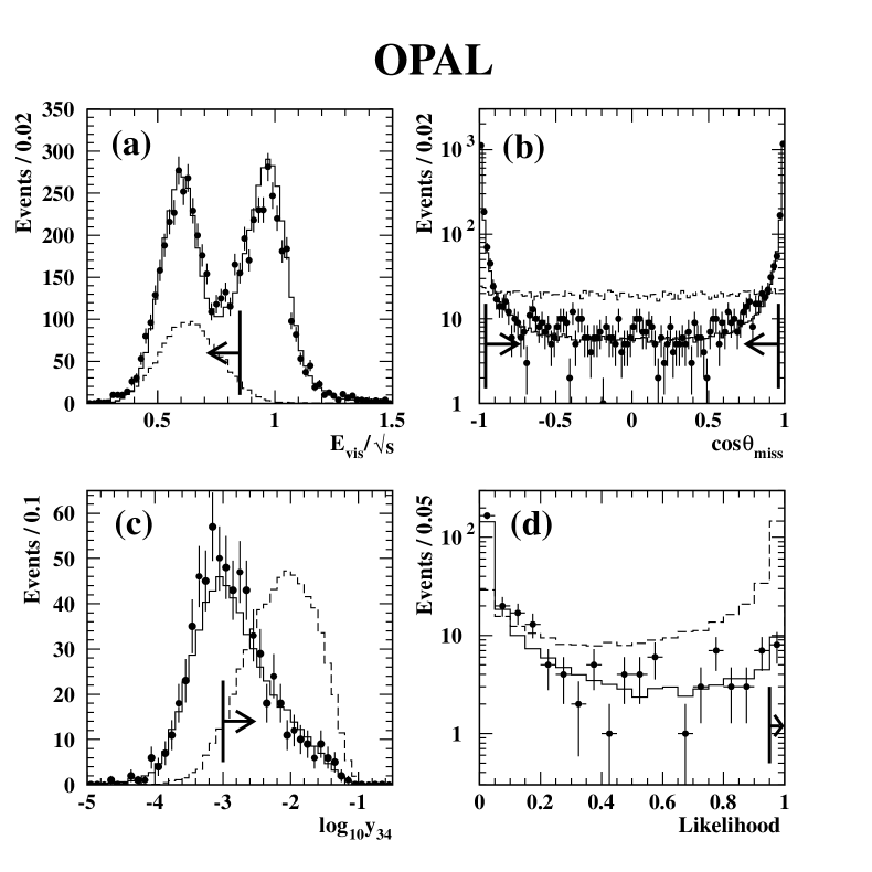
The analysis was optimised to retain good signal efficiency while reducing the background, mainly due to two-photon processes and to $\ell\ell\nu\nu$ final states from ${\mathrm{W}}^{+}{\mathrm{W}}^{-}$ production. The following cuts were applied.

(A1)

Events had to contain exactly two identified and oppositely charged leptons, each with a transverse momentum with respect to the beam axis greater than 2 GeV.

(A2)

The background from two-photon processes and “radiative return” events (${\mathrm{e}}^{+}{\mathrm{e}}^{-}\rightarrow{\mathrm{Z}}\gamma$, where the $\gamma$ escapes down the beam pipe) was reduced by requiring that the polar angle of the missing momentum, $\theta_{\mathrm{miss}}$, satisfied $|\cos\theta_{\mathrm{miss}}|<0.9$.

(A3)

To reduce further the residual background from Standard Model lepton pair events, it was required that $m_{\mathrm{vis}}/\sqrt{s}<0.80$, where $m_{\mathrm{vis}}$ is the event visible mass.

(A4)

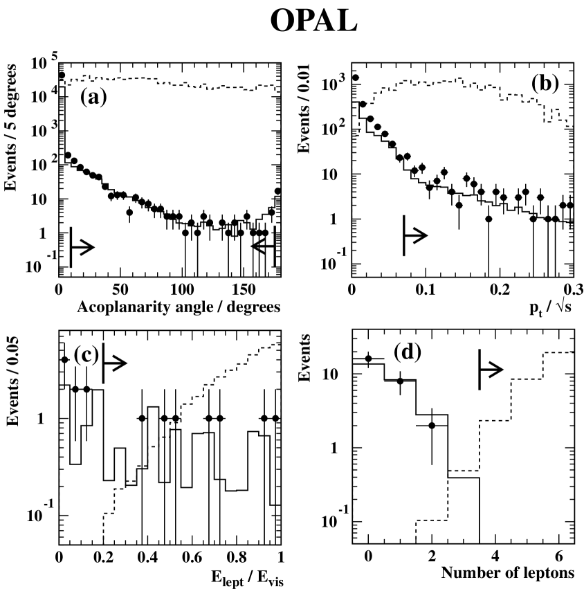
The acoplanarity angle ($\phi_{\mathrm{acop}}$) between the two leptons was required to be greater than 10^∘ in order to reject Standard Model leptonic events, and smaller than 175^∘ in order to reduce the background due to photon conversions. The acoplanarity angle distribution is shown in Figure 2 (a) after cuts (A1) to (A3). The poor agreement between the data and Monte Carlo expectation at this stage of the analysis is due partly to beam related backgrounds and partly to incomplete modelling of two-photon processes. The acollinearity angle ($\theta_{\mathrm{acol}}$) was also required to be greater than 10^∘ and smaller than 175^∘.

(A5)

Cuts on $a_{t}^{\mathrm{miss}}$ and $p_{t}^{\mathrm{miss}}$ were applied, where $a_{t}^{\mathrm{miss}}$ is the component of the missing momentum vector perpendicular to the event thrust axis in the plane transverse to the beam axis and $p_{t}^{\mathrm{miss}}$ is the missing transverse momentum [32, 20].

(A6)

The background was further reduced by requiring that the two identified leptons be of the same flavour. Events were further selected by applying cuts on the momentum of the two leptons as described in [32].

Figure 2: (a) Chargino search (Analysis A): Distribution of the acoplanarity angle. The dotted histogram shows signal Monte Carlo events for direct decays of $\tilde{\chi}^{\pm}_{1}$ with $m_{\tilde{\chi}^{\pm}_{1}}=70$ GeV and for $\lambda$₁₂₂. (b) Neutralino search (Analysis B): Distribution of the event transverse momentum scaled by the centre-of-mass energy and calculated without the hadron calorimeter. The dotted histogram shows signal Monte Carlo events for direct decays of $\tilde{\chi}^{0}_{1}$ with $m_{\tilde{\chi}^{0}_{1}}=70$ GeV and for $\lambda$₂₃₃. (c) Chargino search (Analysis C): Distribution of the energy associated to the identified leptons scaled by the total visible energy. The dotted histogram shows signal Monte Carlo events for indirect decays of $\tilde{\chi}^{\pm}_{1}$ with $m_{\tilde{\chi}^{\pm}_{1}}=70$ GeV and for $\lambda$₂₃₃. (d) Chargino search (Analysis D): Distribution of the number of charged leptons, with a transverse momentum with respect to the beam axis greater than 1.5 GeV. The dotted histogram shows signal Monte Carlo events for direct decays of $\tilde{\chi}^{\pm}_{1}$ with $m_{\tilde{\chi}^{\pm}_{1}}=70$ GeV and for $\lambda$₁₂₂. Data are shown as points and the sum of all Monte Carlo background processes is shown as the solid line. The simulated signal events have arbitrary normalisation. The arrows indicate the cut value.

To maximise the detection efficiencies, the above selection was combined with the standard OPAL analysis to select ${\mathrm{W}}^{+}{\mathrm{W}}^{-}$ pair events [37] where both W’s decay leptonically. This combination was performed after cut (A5) for events passing the preselection criteria. Events passing either set of criteria were accepted as candidates.

Final State	Eff. (%)	Selected Events	Tot. bkg MC	4-fermion
$ee+E_{T\mathrm{miss}}$	44-74	11	13.8	13.5
$\mu\mu+E_{T\mathrm{miss}}$	48-77	10	11.3	11.0
$\tau\tau+E_{T\mathrm{miss}}$	20-45	10	15.5	12.5

Table 4: Detection efficiencies (in %), events selected and background predicted for the lepton-pair plus missing energy channels and for $\tilde{\chi}^{\pm}_{1}$ masses between 45 and 90 GeV.

Detection efficiencies are summarised in Table 4 for the three lepton flavours considered. The efficiencies are quoted for $\tilde{\chi}^{\pm}_{1}$ masses between 45 and 90 GeV. The expected background from all Standard Model processes considered is normalised to the data luminosity of 56.5 pb^-1. As can be seen in Table 4, most of the background remaining comes from 4-fermion processes, expected to be dominated by ${\mathrm{W}}^{+}{\mathrm{W}}^{-}$ doubly-leptonic decays. The second most important contamination for the $\tau\tau$ final states arises from two-photon processes leading to leptonic final states (up to 1.9 events).

5.1.2 Four-Lepton Final States

The following cuts were applied to select a possible signal in the four charged leptons and missing energy topology:

(B1)

The background from two-photon processes and “radiative return” events (${\mathrm{e}}^{+}{\mathrm{e}}^{-}\rightarrow{\mathrm{Z}}\gamma$, where the $\gamma$ escapes down the beam pipe) was reduced by requiring that the polar angle of the missing momentum direction, $\theta_{\mathrm{miss}}$, satisfied $|\cos\theta_{\mathrm{miss}}|<0.9$.

(B2)

At least four tracks with a transverse momentum with respect to the beam axis greater than 1.0 GeV, were required.

(B3)

The event transverse momentum calculated without the hadron calorimeter was required to be larger than 0.07 $\times\sqrt{s}$. This distribution is shown in Figure 2 (b) after cuts (B1) and (B2) have been applied. The poor agreement between the data and Monte Carlo expectation at this stage of the analysis is due partly to beam related backgrounds and partly to incomplete modelling of two-photon processes. When the two-photon processes have been effectively reduced after this cut, the agreement between data and Monte Carlo is good.

(B4)

Events had to contain at least three well-identified isolated leptons, each with a transverse momentum with respect to the beam axis greater than 1.5 GeV.

(B5)

It was required that $E_{\mathrm{vis}}/\sqrt{s}<1.1$.

(B6)

The total leptonic energy, defined as the sum of the energy of all identified leptons, was required to be greater than $0.5\times E_{\mathrm{vis}}$.

(B7)

To reduce further the total background from Standard Model di-lepton production, it was required that the energy sum of the two most energetic leptons be smaller than 0.75 $\times E_{\mathrm{vis}}$.

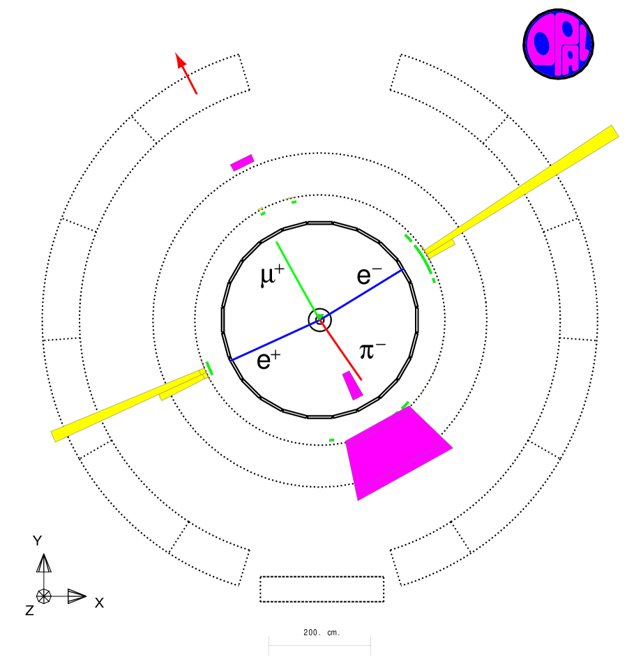
To be independent of the types of decays, direct or indirect, which are searched for and to maximise the detection efficiencies, no specific cut on the lepton flavour present in the final state was applied. Detection efficiencies range from 16% to 74% for neutralino masses between 30 and 90 GeV. The lower efficiency value arises from small neutralino masses (30 GeV) and decays with four taus in the final state. The expected background is estimated to be 2.5 events. One candidate event has been selected from the data; it is shown in Figure 3. This candidate is compatible with pair-production of two on-shell Z bosons, one decaying to an electron pair and the other to a $\tau$ pair. One of the $\tau$’s decays to a pion and a neutrino and the other $\tau$ decays to a muon plus two neutrinos.

Figure 3: Display of the event selected in the data by analysis B. This candidate is compatible with the pair production of two on-shell Z bosons, one decaying to an electron pair and the other to a $\tau$ pair. One of the $\tau$’s decays to a pion and a neutrino and the other $\tau$ decays to a muon plus two neutrinos.

5.1.3 Six-Lepton Final States

The following cuts were applied:

(C1)

To reduce the background from two-photon and di-lepton processes, it was required that $0.1<E_{\mathrm{vis}}/\sqrt{s}<0.7$.

(C2)

The event longitudinal momentum was also required to be smaller than 0.9 $\times{p_{\mathrm{vis}}}$, where ${p_{\mathrm{vis}}}$ is the event total momentum.

(C3)

The event transverse momentum calculated without the hadron calorimeter was required to be larger than 0.025 $\times\sqrt{s}$.

(C4)

Events with fewer than five charged tracks (tracks from photon conversions were not considered) with a transverse momentum with respect to the beam axis larger than 0.3 GeV were rejected.

(C5)

Events had to contain at least three well-identified isolated leptons; at least two of them must have a transverse momentum with respect to the beam axis greater than 1.5 GeV, and the third one must have a transverse momentum with respect to the beam axis greater than 0.3 GeV.

(C6)

The total leptonic energy, defined as the sum of the energy of all identified leptons, was required to be greater than $0.2\times E_{\mathrm{vis}}$. The distribution of the total leptonic energy scaled by the visible energy, is shown in Figure 2 (c), after cuts (C1) to (C4) have been applied.

In the case of final states without missing energy (chargino direct decays without taus), the previous selection cuts were replaced by the following ones:

(D1)

To reduce further the residual background from two-photon processes, it was required that $0.2<E_{\mathrm{vis}}/\sqrt{s}<1.2$.

(D2)

Events with fewer than five charged tracks (tracks from photon conversions were not considered) with a transverse momentum with respect to the beam axis larger than 1 GeV were rejected.

(D3)

Events had to contain at least four well-identified isolated leptons, each of them with a transverse momentum with respect to the beam axis greater than 1.5 GeV. The distribution of the number of charged leptons is shown in Figure 2 (d) after cuts (D1) and (D2) have been applied.

(D4)

The total leptonic energy, defined as the sum of the energy of all identified leptons, was required to be greater than $0.4\times E_{\mathrm{vis}}$.

Events passing either set of criteria were accepted. Detection efficiencies after combining the two analyses range from 22% to 87% for chargino masses between 45 and 90 GeV. The lower value of the selection efficiency arises from decays of a chargino with a mass of 45 GeV leading to final states with 4 taus and two leptons, while the higher value arises from decays of a chargino with a mass of 90 GeV leading to final states with four muons and two electrons. The background expectation is 1.7 events. There is one candidate event selected in the data.

5.1.4 Inefficiencies and Systematic Errors

Variations in the efficiencies were estimated using events generated with $m_{0}$ = 48.4 GeV and also events generated with $\Delta m$ = 5 GeV, as described in Section 3. The inefficiencies due to variation of angular distributions were estimated for five different MSSM parameter sets, representing different neutralino field contents (gaugino/higgsino) and couplings, and calculated separately for each analysis. The selection efficiencies varied by up to 10%. In interpreting the results, a conservative approach was adopted by choosing the lowest efficiencies.

The inefficiency due to forward detector vetoes caused by beam-related backgrounds or detector noise was estimated from a study of randomly triggered beam crossings to be 3.2%. The quoted efficiencies are all scaled down to take this effect into account.

The following systematic errors on the number of signal events expected have been considered : the statistical error on the determination of the efficiency from the Monte Carlo simulation; the systematic error on the integrated luminosity, of 0.35%; the systematic error due to the trigger efficiency was estimated to be negligible because of the high lepton transverse momentum requirement; the uncertainty due to the interpolation of the efficiencies was estimated to be 4.0% and the lepton identification uncertainty was estimated to be 2.4% for muons, 3.9% for electrons and 4.7% for taus. The total systematic error was calculated by summing in quadrature the individual errors. The total systematic error is incorporated into the limit calculation using the method described in Reference [38].

5.2 Jets plus Lepton Final States

The strategy to search for final states with jets and leptons is to look for signals with clear jets and well identified leptons. In the case of neutrinos in the final state, background from two-photon processes can effectively be reduced by requiring some missing transverse momentum. For most decays the leptons will be isolated and therefore well distinguishable from the background. The severest background in most analyses results from W pair production. However a kinematic fit on the invariant mass of jets and leptons gives a good mass resolution and can therefore reduce most of this background.

This section describes the event selection for final states from the direct and indirect decay of gauginos via the couplings $\lambda$  and $\lambda^{{}^{\prime}}$ using an integrated luminosity of 55 pb^-1. The selection cuts are organised as follows:

Preselection

At least seven tracks, a minimum visible energy of 0.3 $\cdot\sqrt{s}$, and at least one identified lepton with at least 3 GeV are required.

(E1)

A cut on the visible energy scaled by the centre of mass energy with values depending on the expected number of neutrinos, in the range between 0.4 and 1.2, is applied. In addition, the angle of the missing momentum with respect to the beam direction has to fulfil $|\cos\theta_{\mathrm{miss}}|<0.95$, if the final state contains neutrinos.

(E2)

The jets in the event have been reconstructed using the Durham [39] algorithm. Cuts have been applied on the number of jets reconstructed with a cut parameter of 0.005, and on the jet resolution $y_{i,i+1}$ at which the number of jets changes from $i$ to $i+1$ jets. The value of $i$ depends on the expected number of jets in the final state, and the cut takes into account the high multiplicity of the signal events.

(E3)

To reduce the background from W pair production for events with missing momentum, a single constrained kinematic fit has been performed. The inputs to the fit are the momenta of the lepton and the neutrino, taking the missing momentum to be the momentum of the neutrino, and the rest of the event reconstructed into 2 jets. The invariant mass is calculated (a) for the lepton and the neutrino system and (b) for the two jet system, letting the masses of both systems be independent. The reconstructed mass of at least one system has to be outside a mass window of 70 GeV$<m<90$ GeV, or the probability for the fit has to be less than 0.01.

(E4)

For the topologies with one charged lepton expected in the final state, the background from W pair production is reduced further by a kinematic fit on the invariant mass of two pairs of jets, when reconstructing the whole event into 4 jets. This kinematic fit assumes energy and momentum conservation and the same mass for both jet pairs. The reconstructed mass has either to be outside a mass window around the W mass, with a width varying between 8 and 20 GeV, depending on the signal to background ratio, or the probability for the fit has to be less than 0.01.

(E5)

For events with only one charged lepton expected from the decay of the $\tilde{\chi}^{\pm}_{1}$ or $\tilde{\chi}^{0}_{1}$, the momentum of the lepton has to be lower than 40 GeV to reduce the background from W pair production.

(E6)

A certain number of identified leptons with a minimum energy is required. For the indirect decay via the coupling $\lambda$ the requirement is at least two leptons with a minimum energy of 10 GeV and 7 GeV for the most and second-most energetic, respectively; for $\lambda^{{}^{\prime}}$ the number of leptons resulting from the $\tilde{\chi}^{0}_{1}$ decay, i.e. 0, 1, or 2. In the direct decays via the $\lambda^{{}^{\prime}}$ coupling also the number of charged leptons expected (i.e. 1 or 2) is required.

(E7)

The identified leptons are required to be isolated. The isolation criterion is that there be no charged track within a cone around the track of the lepton. If two leptons are required, both opening angles have to fulfil $|\cos\theta|<$ 0.99; if only one lepton is required, the opening angle has to fulfil $|\cos\theta|<$ 0.98.

In the following it is described, which of the above cuts has been used for a given analysis. The number of observed and expected events, as well as the efficiencies for each analysis are listed in Table 5.

5.2.1 Indirect Decay via $\lambda$ 

Final states from the $\tilde{\chi}^{\pm}_{1}\$ decay via a W^(∗) can have jets and leptons in the final state. The signature of these final states is at least four isolated leptons plus two or four jets, depending on whether one or both of the W^(∗)’s decay hadronically. If the mass difference between the $\tilde{\chi}^{\pm}_{1}\$ and the $\tilde{\chi}^{0}_{1}\$ becomes small, the jets might not be properly reconstructed. Therefore the analysis is also sensitive to final states with at least two isolated leptons and some additional hadronic activity.

The same cuts are applied for any of the couplings $\lambda$ and also for the final states with two or four hadronic jets from the decays of the two W^(∗). The cuts (E3), (E4), and (E5) have not been applied.

5.2.2 Indirect Decay via $\lambda^{{}^{\prime}}$ 

In the indirect decay of $\tilde{\chi}^{\pm}_{1}$ via $\lambda^{{}^{\prime}}$  there are many different final state topologies possible. The lepton from the $\lambda^{{}^{\prime}}$ decay of the $\tilde{\chi}^{0}_{1}$ can be either charged or neutral. Therefore final states with 2, or 1 charged leptons are analysed separately. The different decay modes of the W^(∗) are all covered with the same cuts. Especially in the region of a small mass difference between the $\tilde{\chi}^{\pm}_{1}$ and the $\tilde{\chi}^{0}_{1}$, all different topologies due to different decay modes of the W^(∗) look similar.

In the final states with two charged leptons from the $\tilde{\chi}^{0}_{1}$ decay, the cuts for electrons and muons are very similar. The cuts (E3), and (E4) have not been applied.

In the selection for final states with one charged lepton, the cuts are the same for all three lepton flavours.

5.2.3 Direct Decay via $\lambda^{{}^{\prime}}$ 

In the direct decay of $\tilde{\chi}^{\pm}_{1}$ and $\tilde{\chi}^{0}_{1}$ via $\lambda^{{}^{\prime}}$ the final states consist of 2 leptons of the same flavour (neutral or charged) plus 4 hadronic jets. The experimental signature is the same for $\tilde{\chi}^{\pm}_{1}$ and for $\tilde{\chi}^{0}_{1}$. Separate analyses have been performed for final states with 1 or 2 charged leptons (electrons or muons). In the case of 2 charged leptons, the cuts (E3), (E4), and (E5) have not been applied.

Figure 4: This figure shows distributions of event variables from the analyses for final states with jets plus leptons for data (points) and MC (full histogram). Also indicated is a signal MC (dashed histogram) for a $\tilde{\chi}^{\pm}_{1}$ of mass 90 GeV, decaying via a $\lambda^{{}^{\prime}}$ coupling into final states with two electrons and a hadronic decay of both W^(∗). The scale of the signal MC is arbitrary. The arrows point into the direction accepted by the cuts applied. (a) The logarithm of the jet resolution, $y_{45}$, at which the number of reconstructed jets changes between 4 and 5, is shown, after the cut on the visible energy has been applied; (b) the number of electrons after the cut on the jet resolution, as indicated in Figure(a), has been applied. (c) The energy of the most energetic electron and (d) the distance between the track of the most energetic electron and the nearest track, $\Delta_{\mathrm{track}}$, requiring at least two identified electrons.

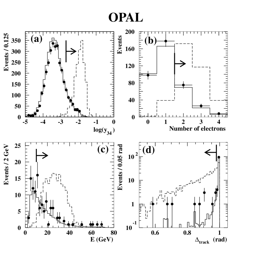
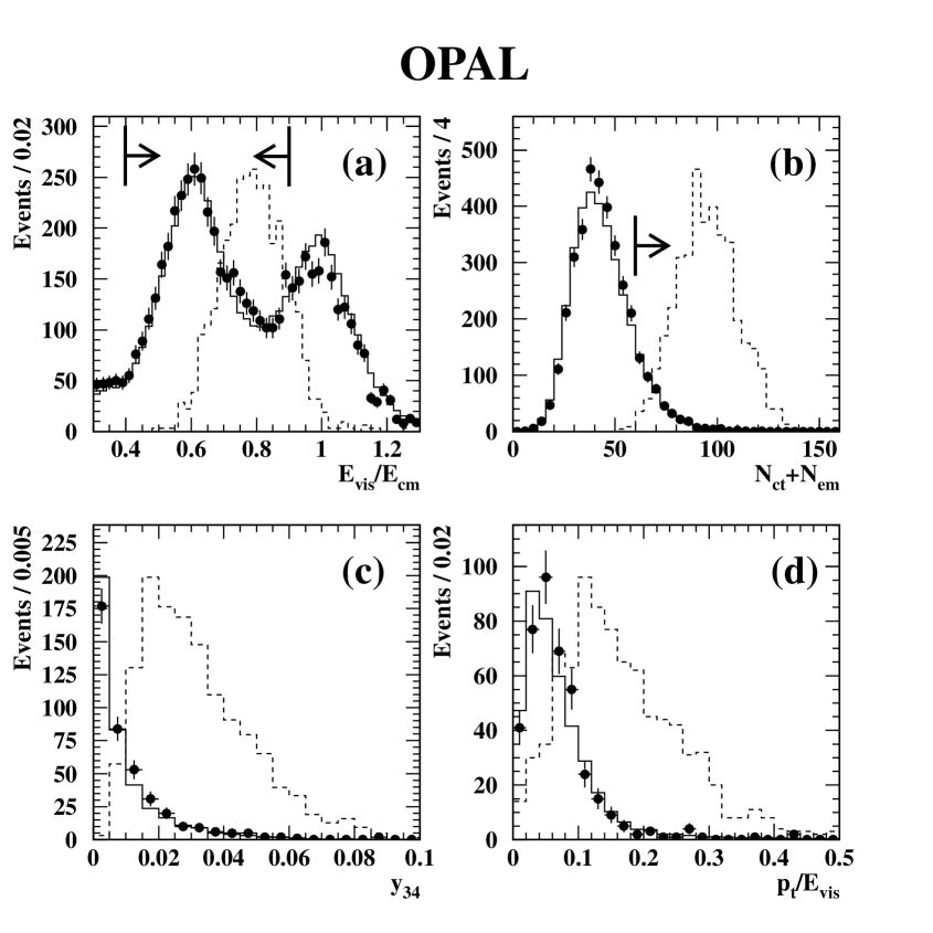
For the decay mode of a $\tilde{\chi}^{\pm}_{1}$ via the coupling $\lambda^{{}^{\prime}}$ into a final state with two electrons the event distributions and several of the cuts used are shown in Figure 4. The signal is shown for a $\tilde{\chi}^{\pm}_{1}$ of 90 GeV and the hadronic decay mode of the W^(∗)’s, but the cuts are the same for all decay modes of the W^(∗)’s. Therefore the data distributions do not depend on it.

Figure 4(a) shows the event distributions for the visible energy, scaled by the centre of mass energy after the preselection cuts. The lower cut is chosen so that also the leptonic decay mode of the W^(∗)’s is selected. Figure 4(b) shows the jet resolution, $y_{4}$, where the number of jets changes from 4 to 5 jets after the cut on the visible energy has been applied. For Figures 4(c) and (d) the cuts up to (E5) have been applied and show the number of electrons and the distance of the most energetic electron with respect to the closest track, respectively.

5.2.4 Efficiencies and Backgrounds

The efficiencies resulting from the analyses above lie between 30 and 80% for final states without at least one electron or muon from the $\tilde{\chi}^{0}_{1}$ decay for $\tilde{\chi}^{\pm}_{1}$ masses around 90 GeV. For final states with taus the efficiencies lie in the range between 10% and 30%. The efficiencies are best for the topologies resulting from the decays via couplings $\lambda$, as many well isolated leptons are present. Also the topologies with two electrons or two muons in the indirect decays via $\lambda^{{}^{\prime}}$ have efficiencies above 50% for $\tilde{\chi}^{\pm}_{1}$ masses of 90 GeV.

Final State	Eff. (%)	Selected Events	Tot. bkg MC
$\lambda$ indirect	12 – 82	1	3.3
$\lambda^{{}^{\prime}}$ indirect
$ee+\geq$ 4 jets	23 – 55	1	1.4
$e\nu+\geq$ 4 jets	3 – 30	0	1.0
$\mu\mu+\geq$ 4 jets	27 – 60	0	1.5
$\mu\nu+\geq$ 4 jets	3 – 31	2	0.5
$\tau\nu+\geq$ 4 jets	1 – 11	6	4.9
$\lambda^{{}^{\prime}}$ direct
$ee$ + 4 jets	24 – 57	1	0.9
$e\nu$ + 4 jets	7 – 39	1	2.0
$\mu\mu$ + 4 jets	30 – 60	0	1.0
$\mu\nu$ + 4 jets	8 – 46	4	1.4
$\tau\nu$ + 4 jets	2 – 14	1	4.1

Table 5: Detection efficiencies (in %) for the final states considered for $\tilde{\chi}^{\pm}_{1}$ masses varying between 45 and 90 GeV and for $\tilde{\chi}^{0}_{1}$ masses between 30 and 90 GeV. The number of events remaining after the selection cuts and the expected backgrounds from all Standard Model processes considered are quoted. The main contribution to the total background estimate derives from ${\mathrm{W}}^{+}{\mathrm{W}}^{-}$ leptonic decays (4-fermion processes), while other processes contribute less than 10%.

The background from two-photon processes is negligible, same as the background from multihadronic final states for most analyses. W pair production is the major background. The number of expected background events is estimated to be between 0.5 and 2.0 for events with at least one electron or muon from the $\tilde{\chi}^{0}_{1}$ decay. For events with taus from the $\tilde{\chi}^{0}_{1}$ decay, the expected background lies in between 1.6 and 4.9 events, and 2.9 events are expected in the case of no charged lepton in the decay of the $\tilde{\chi}^{0}_{1}$.

The numbers of events observed in the data show no significant discrepancy over the expected number of events.

5.2.5 Systematic Errors

For the lepton identification a systematic error of 4% was estimated for the electrons, 3% for the muons and 6% for the taus. The systematic error on the measured luminosity is 0.35%. The systematic error due to the uncertainty in the trigger efficiency was estimated to be negligible, because of the requirement of at least seven good tracks. The statistical error on the determination of the efficiency from the MC samples has also been treated as a systematic error. To check the dependence on the quark flavour of the jets, samples with different quark flavours have been produced. The standard samples used to determine the efficiencies always resulted in the lowest efficiency. Therefore no additional error has been assigned due to the quark flavour.

5.3 Jets Plus Two $\tau-$Lepton Final States

Final states containing at least two $\tau$-leptons and between four and eight jets can be produced via the processes e⁺e${}^{-}\rightarrow\tilde{\chi}^{\pm}_{1}\tilde{\chi}^{\pm}_{1}$ or $\tilde{\chi}^{0}_{1}\tilde{\chi}^{0}_{1}$, with $\chi\rightarrow\tau+qq$. In the case of direct decay, and $\chi^{\pm}\rightarrow\chi^{0}f\bar{f^{\prime}}\rightarrow\tau+qq+f\bar{f^{\prime}}$ in the case of indirect decay, leading to the following four possible signal topologies:

• Direct decay:

  (a)

  four jets and two $\tau$-leptons

• Indirect decay:

  (b)

  four jets, two $\tau$-leptons plus two additional leptons (of any flavour) and their associated neutrinos

  (c)

  six jets, two $\tau$-leptons plus one additional lepton (of any flavour) and its associated neutrino

  (d)

  eight jets and two $\tau$-leptons

The backgrounds come predominantly from ($Z\gamma)^{*}\rightarrow q\bar{q}(\gamma)$ and four-fermion processes.

In each of the four cases, the selection begins with the identification of $\tau$-lepton candidates [40], using three algorithms designed to identify electronic,muonic and hadronic $\tau$-lepton decays. The original $\tau$-lepton direction is approximated by that of the visible decay products. The following preselection, was made:

(F1)

Events are required to contain at least nine charged tracks, and must have at least two $\tau$-lepton candidates, each with electric charge $|q|=1$ and whose charges sum to zero.

(F2)

Events must have no more than a total of 20 GeV of energy deposited in the forward detector, gamma-catcher, and silicon-tungsten luminosity monitor; a missing momentum vector satisfying $|\cos\theta_{\rm miss}|<0.97$, total vector transverse momentum of at least 2% of $\sqrt{s}$, and a scalar sum of all track and cluster transverse momenta larger than 40 GeV.

(F3)

Events must contain at least three jets, reconstructed using the cone algorithm as in [40], and no energetic isolated photons.

(F4)

Events must contain no track or cluster with energy exceeding $0.3\sqrt{s}$.

In order to select a final $\tau$-candidate pair for each event, and to further suppress the remaining background, a likelihood method similar to that described in [44] is applied to those events passing the above preselection. For each $\tau$-candidate pair and its associated hadronic “rest of the event” (RoE), composed of those tracks and clusters not having been identified as belonging to the pair, a joint discriminating variable, ${\cal L}$, is constructed using normalised reference distributions generated from Monte Carlo samples of events belonging to the following four classes:

1. Signal events where the selected pair is composed of two real $\tau$-leptons

2. Signal events where the selected pair contains at most one real $\tau$-lepton

3. SM four-fermion events where the selected pair is composed of up to two real $\tau$-leptons

4. Events from the process $Z\gamma^{*}\rightarrow q\bar{q}(\gamma)$ containing no real $\tau$-leptons

For classes 1 and 2, different signal reference distributions are generated for the four topologies a)-d). The variable ${\cal L}$ is related to the probability that the selected $\tau$-candidate pair and RoE belong to class 1. The set of input variables to the reference distributions includes those which characterise each of the two $\tau$-lepton candidates individually, those which describe their behaviour as a pair and those which characterise the RoE. For those variables describing the $\tau$-candidates individually, separate reference distributions are generated for leptonic (electron or muon), hadronic 1-prong and hadronic 3-prong $\tau$-candidates, in order to exploit the differences between the three categories, as follows:

• Used for all three categories:

  • $|\cos\alpha_{i}|$, where $\alpha_{i}$ is the angle between the direction of the $i$-th $\tau$ candidate and that of the nearest track not associated with it.

  • $|\vec{p}_{i}|$, the momentum of this nearest non-associated track

  • $R_{em}^{11/30}\cdot R_{cd}^{11/30}$, where $R_{em(cd)}^{11/30}$ is the ratio of the electromagnetic cluster energies (charged track momenta) within a cone of $11^{\circ}$ half-angle centred on the $\tau$ candidate axis to that within a $30^{\circ}$ half-angle cone.

  • $|\vec{p}_{\tau}|$, the magnitude of the momentum of the $\tau$-candidate.

  • The type of $\tau$ candidate itself, i.e. lepton, 1-prong, 3-prong.

• Used for 1- and 3-prong categories:

  • $\sum_{i}|p_{T}|_{i,\tau}/E_{\tau}$, the sum of the transverse momenta (with respect to the $\tau$-candidate axis) of tracks $i$ in the $\tau$-candidate

  • $m_{\tau}$, the invariant mass of the $\tau$ candidate

• Used for lepton and 1-prong categories:

  • The magnitude of the impact parameter, in three dimensions, of the $\tau$-candidate

• Used for 1-prong category only:

  • $N_{hd}/N_{em}$, the ratio of hadronic calorimeter to electromagnetic calorimeter clusters associated to the $\tau$ candidate.

• Used for 3-prong category only:

  • The vertex significance in three dimensions of the $\tau$-candidate.

Figure 5: Jets plus at least two $\tau$-leptons, topology a): Distributions of relevant quantities for data(points), estimated SM background (full histogram) normalised to the integrated luminosity of the data, and a simulated signal (dashed histogram, arbitrary normalisation) corresponding to $m_{\chi^{\pm}}=70$ GeV (direct decay). Figures (a),(b) and (c) show some of the variables input to the likelihood: (a) The momentum of leptonic $\tau$ candidates; (b)The momentum of 1-prong hadronic $\tau$ candidates; (c) The sphericity of the hadronic RoE. The likelihood distribution ${\cal L}$ is shown in (d); events to the right of the arrow indicating the cut position are accepted. All distributions are after the imposition of cut (F4).

The following five input variables are used to characterise the $\tau$-candidates as a pair or the RoE associated with the pair:

• The angle between the two $\tau$-candidates

• The sphericity of the RoE

• The sum of the number of charged tracks and electromagnetic calorimeter clusters in the RoE

• The number of hadronic calorimeter clusters in the RoE

• The jet resolution parameter $y_{23}^{RoE}$, at which the number of jets in the RoE changes from 2 to 3.

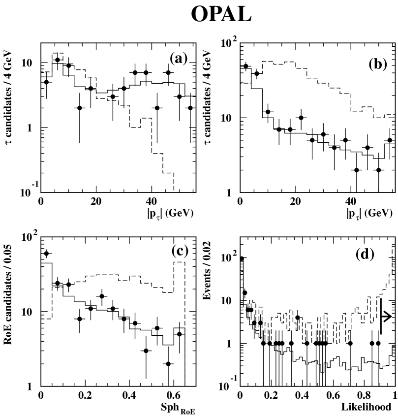
Distributions of some of the input variables as well as that of ${\cal L}$ are shown in Fig. 5, for the case of topology a).

The $\tau$-candidate pair having the highest value of ${\cal L}$ is chosen in each event. Then, for topology b) only, the following requirement is imposed reflecting the expectation of two additional leptons other than the two $\tau$-leptons:

(F5)

The sum of the number of $\tau$-lepton candidates plus the number of identified electrons (as in [40]) and muons not tagged as $\tau$-lepton candidates must be at least 4.

Finally, the following requirements are made on the values of ${\cal L}$:

(F6)

${\cal L}>0.9,0.6,0.65$ and $0.75$ respectively for signal topologies a), b), c), d).

For topologies a)-d) respectively, zero, two, one and one events survive the selection while the background is estimated to be 2.27, 2.31, 3.19 and 1.93 events for an integrated luminosity of 55.8 pb^-1. The detection efficiencies for chargino masses between 70 and 90 GeV range from approximately 24 to 28%, 21 to 32%, 22 to 24%, and 14 to 19%, while those for neutralinos in the same mass range lie between 17 and 18%. For charginos with masses of 45 GeV and below, the detection efficiency falls to approximately 5%, 9%, 5% and 1%, and for neutralinos to (8%).

These efficiencies are affected by the following uncertainties: Monte Carlo statistics, typically 5.0%; uncertainty in the tau-lepton preselection efficiency, 1.2%; uncertainty in the modelling of the other preselection variables, 2.0%; uncertainties in the modelling of the likelihood input variables, 10.0%; uncertainties in the modelling of fragmentation and hadronisation, 6.0%; and uncertainty on the integrated luminosity, 0.5% [41]. Taking these uncertainties as independent and adding them in quadrature results in a total systematic uncertainty of 12.9% (relative errors). The uncertainty in the number of expected background events was estimated to be 18%.

5.4 Four Jets plus Missing Energy

Direct decays of charginos and neutralinos via $\lambda^{\prime}$ coupling can lead to final states with four jets and missing energy due to the two undetected neutrinos. The dominant backgrounds come from four-fermion processes and radiative or mismeasured two-fermion events. The selection procedure is described below:

(G0)

The event has to be classified as multi-hadron final-state as described in [42].

(G1)

The visible energy of the event is required to be less than 0.85$\sqrt{s}$.

(G2)

To reject two-photon and radiative two-fermion events the transverse momentum should be larger than 10 GeV, the total energy measured in the forward calorimeter, gamma-catcher and silicon tungsten calorimeter should be less than 20 GeV, and the missing momentum should not point to the beam direction, $|\cos\theta_{\mathrm{miss}}|<$ 0.96.

(G3)

The events are forced into four jets using the Durham jet-finding algorithm, and rejected if the jet resolution parameter $y_{34}$ is less than 0.001.

(G4)

An additional cut is applied against semi-leptonic four-fermion events, vetoing on isolated leptons being present in the event. The lepton identification is based on an Artificial Neural Network routine [43], which was originally written to identify tau leptons but is efficient for electrons and muons, as well. The ANN output is required to be larger than 0.97 for lepton candidates.

(G5)

Finally, a likelihood selection is employed to classify the remaining events as two-fermion, four-fermion or qqqq$\nu\nu$ processes. The method is described in [44]. The information of the following variables are combined:

• the effective centre-of-mass energy [45] of the event;

• the transverse momentum of the event;

• the cosine of the polar angle of the missing momentum vector;

• the D parameter [46] of the event;

• the logarithm of the $y_{34}$ parameter;

• the minimum number of charged tracks in a jet;

• the minimum number of electromagnetic clusters in a jet;

• the highest track momentum;

• the highest electromagnetic cluster energy;

• the number of leptons in the event, using loose selection criteria for the lepton candidates (the ANN output is larger than 0.5);

• the mass of the event excluding the best lepton candidate (if any) after a kinematic fit using the W⁺W^- $\rightarrow$ qq$l\nu$ hypothesis;

• the cosine of the smallest jet opening angle, defined by the half- angle of the smallest cone containing 68% of the jet energy;

The event is rejected if its likelihood output is less than 0.95.

Figure 6 shows experimental plots of the selection variables for the data, the estimated background and simulated signal events. The distributions are well described by the Monte Carlo simulation.

Figure 6: Four jets plus missing energy: Distributions for data (points), for the estimated SM background (full histogram) and for simulated signal (dotted histogram). Figure (a) shows the visible energy, E_vis, scaled by the centre of mass energy, $\sqrt{s}$, for multihadron events after cut (G0). In Figure (b) the cosine of the polar angle of the missing momentum vector is plotted after cut (G1). In Figure (c) the logarithm of the jet resolution, $y_{34}$, at which the number of reconstructed jets changes between 3 and 4, is shown after cut (G2) have been applied. Figure (d) shows the final selection using the likelihood output. The arrows indicate the accepted regions in each plot. The SM background is normalised to the integrated luminosity of the data, while the normalisation of the signal distribution is arbitrary.

After all cuts, 8 events are selected in the data sample, while 9.47$\pm$ 0.33 (stat) $\pm$ 2.07 (syst) events are expected from Standard Model processes, of which 72% originates from four-fermion processes. The signal detection efficiency varies between 7% and 60% for gaugino masses of 45 – 90 GeV for $\lambda^{\prime}_{121}$ and $\lambda^{\prime}_{123}$ couplings.

The small efficiency for light gaugino masses is the result of initial-state radiation and the larger boost of the particles, which make the event similar to the QCD two-fermion background.

The background expectation is subject to the following systematic errors and inefficiencies: inefficiency due to the forward energy veto (1.8%); the statistical error due to the limited number of Monte Carlo events (3.4%); the statistical and systematic error on the luminosity measurement (0.45% in total); error on the lepton veto (1%); uncertainty on modelling the SM background processes by comparing different event generators (3.3%) and the modelling of kinematic variables used in the analysis (21%, dominated by the error on the visible energy).

The signal detection efficiency is affected by the following systematics: inefficiency due to the variation of m₀ (0 – 5%) and due to the forward energy veto (1.8%); the statistical error due to the limited number of Monte Carlo events (2 – 12%); error on the lepton veto (1%); uncertainty on modelling the kinematic variables used in the analysis (6%).

5.5 More than Four Jets plus Missing Energy

This analysis applies to chargino indirect decays via $\lambda^{{}^{\prime}}$, where both neutralinos decay into quarks and neutrinos. The selected events must have clear reconstructed jets, missing energy and missing transverse momentum. To account for the possibility of leptonic decays of the W^(∗), the presence of charged leptons in the events has to be allowed; an upper bound on the lepton momentum is imposed, in order to reduce the background from semi-leptonic W-pair events.

The total integrated luminosity amounts to 56.5 pb^-1. The selection cuts are described below. An event is retained as a candidate if it satisfies the Preselection and any of the requirements (H1), (H2) or (H3).

Preselection

Events have to be classified as multi-hadron final states as described in [42]. The visible energy $E_{\mathrm{vis}}$, scaled by the centre-of-mass energy must be in the range $0.4<E_{\mathrm{vis}}/\sqrt{s}<0.9$. The most energetic identified lepton (e or $\mu$) must have a momentum lower than 25 GeV. The number of tracks plus the number of EM clusters must exceed 60.

(H1)

The jet resolution $y_{34}$, at which the event switches from 3 to 4 jets, must be $y_{34}>0.02$. The missing momentum $p_{t}$ of the event, scaled by the visible energy, must satisfy $p_{t}/E_{\mathrm{vis}}>0.15$.

(H2)

To increase the efficiency for small $\Delta m$ values, where the missing energy is larger but some jets are softer, $y_{34}>0.015$ and $p_{t}/E_{\mathrm{vis}}>0.2$ are required.

(H3)

To improve the efficiency for $m_{\tilde{\chi}^{\pm}_{1}}=45$ GeV, where many events are affected by initial state radiation and have therefore smaller visible energy and softer jets, $E_{\mathrm{vis}}/\sqrt{s}<0.7$, $y_{34}>0.01$ and $p_{t}/E_{\mathrm{vis}}>0.13$ are required.

Figure 7: Distributions of event variables for final states with more than four jets and missing energy, for data (points) and MC (full histogram). Also indicated is a signal MC (dashed histogram) for $\tilde{\chi}^{\pm}_{1}$ pairs of mass 90 GeV and $\Delta m=45$ GeV. Both charginos are assumed to decay indirectly via a $\lambda^{{}^{\prime}}$ coupling into $\nu$qq, and both W^(∗) into hadrons, leading to qq qq $\nu$qq $\nu$qq final states. The scale of the signal MC is arbitrary. (a) Visible energy scaled by the centre-of-mass energy, $E_{\mathrm{vis}}/\sqrt{s}$, for events selected as multi-hadron final states. The lower cut rejects $\gamma\gamma$ events. (b) The number of charged tracks $N_{ct}$ plus the number of EM clusters $N_{em}$, after all the other cuts of the preselection. (c) The jet resolution parameter $y_{34}$ at which the number of reconstructed jets switches between 3 and 4, plotted after the preselection cuts. (d) The event transverse momentum $p_{t}$ scaled by the visible energy $E_{\mathrm{vis}}$, plotted after the preselection cuts. In Figures (a) and (b) the arrows point to the region accepted by the applied cuts.

The distributions of the selection variables are shown in Figure 7 for experimental data, Standard Model background and signal. After the full selection 7 events survive, where the expected background from Standard Model is 10.9 events. The efficiency is in the range 6% – 33%.

The systematic error due to the Monte Carlo statistics is less than 1.5%; the systematic error on the collected luminosity is 0.35%; the systematic error due to the trigger efficiency is assumed to be negligible, due to the large track and cluster multiplicity required. The total systematic error due to the applied cuts is 2.3%, where the most relevant components arise from the cuts on $y_{34}$ (2.2%) and $p_{t}/E_{\mathrm{vis}}$ (0.6%).

The sensitivity of the selection to quark flavours has been studied, showing that final states containing heavy quarks yield larger efficiencies; conservatively, the quark flavours yielding the lowest efficiencies have been considered to evaluate limits. The variation in the efficiency due to variations in $m_{0}$ and $\Delta m$ has been studied and the lowest efficiency has been used.

5.6 More than Four Jets and No Missing Energy

This analysis applies to chargino direct and indirect decays via $\lambda^{{}^{\prime\prime}}$. Events are expected to have at least six quarks in the final state. The event thrust and sphericity are also used to reduce the background.

Figure 8: Distributions of event variables for final states with more than four jets, for data (points) and MC (full histogram). Also indicated is a signal MC (dashed histogram) for $\tilde{\chi}^{\pm}_{1}$ pairs of mass 90 GeV, decaying directly via $\lambda^{{}^{\prime\prime}}$ coupling into $\mathrm{qqq~{}qqq}$ final states. The scale of the signal MC is arbitrary. (a) Thrust distribution, plotted after the preselection cuts. (b) Sphericity distribution, plotted after the cut on the thrust. (c) Distribution of the jet resolution parameter $y_{34}$ at which the number of reconstructed jets switches between 3 and 4, plotted after the cut on the sphericity. (d) Distribution of $y_{45}/y_{34}$, plotted after the cut on $y_{34}$. In each figure, the arrows point to the region accepted by the applied cut.

The total collected luminosity amounts to 56.5 pb^-1. The selection cuts are described below. An event is retained as a candidate if it satisfies the Preselection and any of the two requirements (I1) or (I2).

Preselection

Events have to be classified as multi-hadron final states as described in [42]. The visible energy $E_{\mathrm{vis}}$, scaled by the centre-of-mass energy, must be in the range $E_{\mathrm{vis}}/\sqrt{s}>0.4$.

(I1)

To reduce the ${\mathrm{q}}\bar{\mathrm{q}}$ background, an event $\mathrm{thrust}$ less than 0.9 and a $\mathrm{sphericity}$ larger than 0.2 are required. To reduce ${\mathrm{q}}\bar{\mathrm{q}}$, ${\mathrm{q}}\bar{\mathrm{q}}\ell\nu$ events, $y_{34}>0.02$ is required. To reduce ${\mathrm{q}}\bar{\mathrm{q}}{\mathrm{q}}\bar{\mathrm{q}}$ events, $y_{45}/y_{34}>0.5$ is required.

(I2)

To reduce 4-fermion events and part of two-jet ${\mathrm{q}}\bar{\mathrm{q}}$ events, $0.8<\mathrm{thrust}<0.9$ is required. To reduce ${\mathrm{q}}\bar{\mathrm{q}}$ events, $y_{56}>0.003$ is required.

The condition (I1) is optimised for large chargino masses, but becomes inefficient for smaller masses, where the chargino decay products are very boosted, and jets cannot be easily resolved. The condition (I2) recovers efficiency in this latter case, exploiting the sharper thrust distribution, due to the large boots.

Figure 9: Distributions of event variables for final states with more than four jets, for data (points) and MC (full histogram). Also indicated is a signal MC (dashed histogram) for $\tilde{\chi}^{\pm}_{1}$ pairs of mass 45 GeV, decaying directly via $\lambda^{{}^{\prime\prime}}$coupling into $\mathrm{qqq~{}qqq}$ final states. The scale of the signal MC is arbitrary. (a) Thrust distribution, plotted after the preselection cuts. (b) Distribution of the jet resolution parameter $y_{56}$ at which the number of reconstructed jets switches between 5 and 6, plotted after the cut on the thrust. In each figure, the arrows point to the region accepted by the applied cut.

The distributions of the selection variables are shown in Figures 8 and 9, for experimental data, Standard Model background and signal. After the selection, 24 events survive, where the expected background from Standard Model is 22.4 events. The efficiency is in the range 9% – 23%.

The systematic error due to the Monte Carlo statistics is less than 1.4%; the systematic error on the integrated luminosity is 0.35%; the systematic error due to the trigger efficiency is assumed to be negligible, due to the large track and cluster multiplicity required.

The variation in the efficiency due to variations in $m_{0}$ and $\Delta m$ has been studied and the lowest efficiency has been used. The sensitivity of the selection to quark flavours has been studied, showing that final states containing heavy quarks yield larger efficiencies; conservatively, the quark flavours yielding the lowest efficiencies have been considered to evaluate limits.

The total systematic error due to the applied cuts is 4.0%, where the most relevant components arise from the cuts on $y_{34}$ (2.2%) and $y_{45}/y_{34}$ (3.3%). The systematic error due to the incorrect simulation of the parton shower for quark triplets, such as those originating from gaugino decays, is estimated to be 1.2%.

6 Limits on Topological Cross-Sections

In this chapter the results from the individual topological analyses presented in the previous chapter are given. As for each topological search the observation is in good agreement with the Standard Model expectations, there is no claim for a signal, and 95% confidence level (CL) cross-section upper limits are presented for final state topologies expected from $R$-parity violating $\tilde{\chi}^{\pm}_{1}$ and $\tilde{\chi}^{0}_{1}$ decays.

6.1 Multilepton Final States

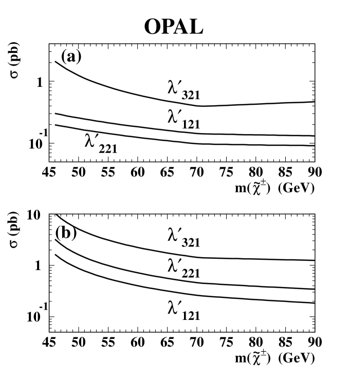
Figure 10 shows the upper limits obtained for the cross-section times branching ratio of leptonic final states from the selection described in Section 5.1. In each of the Figures 10(a), (b), (c), corresponding to two-, four-, and six-lepton final states, the two curves represent the cross-section limits for lepton flavour mixtures yielding the most and the least stringent limits; the latter usually corresponds to several taus in the final state. The limits corresponding to any other lepton flavour mixture are located within the band between the two curves. The specific couplings $\lambda_{ijk}$ which lead to the limiting curves are indicated in each case.

Figure 10: Upper limits at 95% CL on the cross-sections for final states with (a) 2 leptons, (b) 4 leptons, and (c) 6 leptons. For each curve the coupling $\lambda$ that was assumed to be different from zero is given. Limits arising from any other coupling $\lambda$ different from zero lie in the band between the two curves.

6.2 Final States with Leptons plus Jets

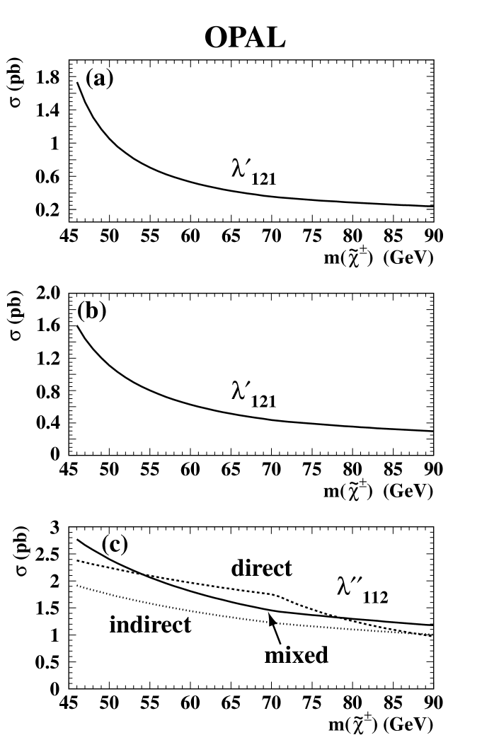
Figures 11, 12, and 13 show the cross-section limits for final states with leptons plus jets from the selections described in Sections 5.2 and 5.3. Figure 11 corresponds to final states with (a) five charged leptons plus two jets and (b) four charged leptons plus four jets. Again, the limits obtained for various mixtures of lepton flavours lie in the band between the two limiting curves. Figure 12 corresponds to final states with (a) two charged leptons of the same flavour plus four jets and (b) one charged lepton plus four jets. Here the limits are given separately for each of the lepton flavours, fixed by the first index of the coupling $\lambda_{ijk}^{{}^{\prime}}$. Limits arising from any other coupling $\lambda^{{}^{\prime}}$ lie below the limit shown for the coupling with the same first index. The final states shown in Figure 13 are like the ones in Figure 12 plus the decay products of two W^(∗). Again, the limits are given separately for each of the lepton flavours, fixed by the first index of the coupling $\lambda_{ijk}^{{}^{\prime}}$ and limits arising from any other coupling $\lambda^{{}^{\prime}}$ lie below the limit shown for the coupling with the same first index.

Figure 11: Upper limits at 95% CL on the cross-sections for final states with jets and leptons resulting from the indirect decay via a coupling $\lambda$. In the upper plot one W^(∗) is decaying leptonically and the other hadronically, while in the lower plot both decay hadronically. For each curve, the coupling $\lambda$ that was assumed to be different from zero is indicated. Limits arising from any other coupling $\lambda$ different from zero lie in the gray zone between the two curves shown.

Figure 12: Upper limits at 95% CL on the cross-sections for final states with jets and leptons resulting from the direct decay via a coupling $\lambda^{{}^{\prime}}$ for (a) two lepton plus four jets final states and (b) for one lepton plus four jets final states. For each curve the coupling $\lambda^{{}^{\prime}}$ that was assumed to be different from zero is given. Limits arising from any other coupling $\lambda^{{}^{\prime}}$ lie below the limit shown for the coupling with the same first index.

Figure 13: Upper limits at 95% CL on the cross-sections for final states with jets and leptons resulting from the indirect decay via a coupling $\lambda^{{}^{\prime}}$. In Figure (a) final states with two charged leptons of the same flavour are shown. Figure (b) shows the final states with one charged lepton. Each Figure contains all decay modes of the two W^(∗). For each curve the coupling $\lambda^{{}^{\prime}}$ that was assumed to be different from zero is given. Limits arising from any other coupling $\lambda^{{}^{\prime}}$ lie below the limit shown for the coupling with the same first index.

6.3 Multi-jet Final States

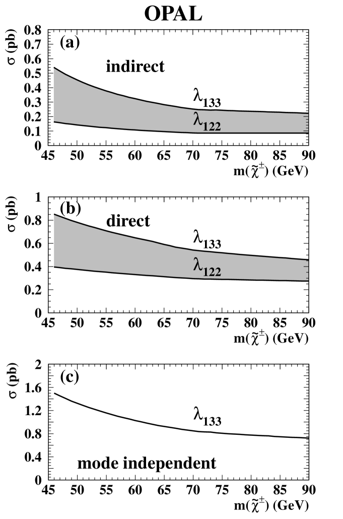
Figure 14 shows the cross-section limits for final states with at least four jets from the selections described in Sections 5.4, 5.5, and 5.6. Figure 14 (a) corresponds to final states with four jets plus missing energy and (b) to four jets plus missing energy plus two W^(∗). The limits shown are independent on the first index of the coupling $\lambda_{ijk}^{{}^{\prime}}$, corresponding to the neutrino flavour. Limits arising from any other coupling $\lambda^{{}^{\prime}}$ lie below the limit shown. In Figure 14 (c) limits for final states with at least six jets are shown. The three limits labelled direct, mixed, and indirect correspond to final states with six jets plus 0, 1, and 2 W^(∗), respectively. Limits arising from any other coupling $\lambda^{{}^{\prime\prime}}$ lie below the limits shown.

Figure 14: Upper limits at 95% CL on the cross-sections for final states with (a) four jets and missing energy, (b) four jets and missing energy plus two W^(∗), and (c) at least six jets. For each curve the coupling $\lambda^{{}^{\prime}}$ or $\lambda^{{}^{\prime\prime}}$ that was assumed to be different from zero is given. Limits arising from any other coupling $\lambda^{{}^{\prime}}$ or $\lambda^{{}^{\prime\prime}}$ lie below the limits shown.

7 Limits on the Gaugino Production Cross-Sections

We now proceed to derive upper bounds on the cross-section of the processes e⁺e${}^{-}\rightarrow\tilde{\chi}^{+}_{1}\tilde{\chi}^{-}_{1}$ and $\tilde{\chi}^{0}_{1}\tilde{\chi}^{0}_{1}$. These are presented separately for the direct and indirect modes for decays being mediated by the couplings $\lambda$, $\lambda^{{}^{\prime}}$, and $\lambda^{{}^{\prime\prime}}$. In addition a limit independent of a decay via the direct or indirect mode is given. The limits are valid for values of the couplings $\lambda$, $\lambda^{{}^{\prime}}$, and $\lambda^{{}^{\prime\prime}}$ greater than 10^-5, assuming a prompt decay at the interaction vertex. Further requirements are that the mass difference $\Delta m=m(\tilde{\chi}^{\pm}_{1})-m(\tilde{\chi}^{0}_{1})$ be larger than 5 GeV, and that only one $\lambda$-coupling be different from zero. For the indirect decay of the $\tilde{\chi}^{\pm}_{1}$, we assume the decay via a W^(∗), and combine the results according to the leptonic and hadronic branching ratio of the W boson. Decays via a sfermion are not considered in this analysis.

The likelihood ratio method [47] has been used to combine the results from several analyses to determine the excluded cross-sections. This method assigns a greater weight to analyses with a higher expected sensitivity, taking into account the expected background. All upper bounds on the cross-sections are given at the 95% CL.

The same method has been used in the determination of limits which are independent of whether the decay is direct or indirect. The branching fractions into these two decay modes varies with the parameters of the MSSM. To achieve a limit independent of the branching ratio and thus of the MSSM parameters, the branching fractions into the direct and indirect decays have been varied simultaneously between 0 and 1. The efficiency for the process of one chargino decaying via the direct mode and the other via the indirect mode has been set to zero, except for the case of $\lambda^{{}^{\prime\prime}}$. A limit is then calculated for all branching ratios at each mass value using the likelihood ratio method. This results in a cross-section limit as a function of the branching ratio and the chargino mass. By taking the worst limit at each mass value, a limit independent of the branching ratio is determined.

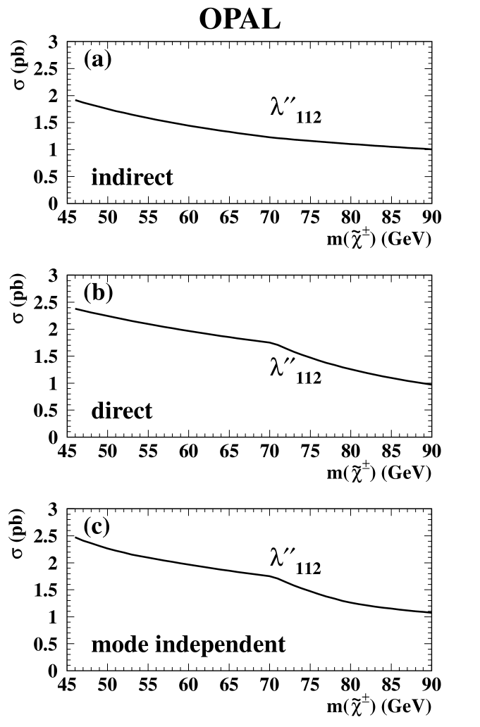
7.1 Chargino Decays via $\lambda$

Figure 15 shows the upper limits on the cross-sections for decays via a coupling $\lambda$ for (a) the indirect decay (b) the direct decay and (c) independent of the decay mode. The upper limits on the cross-section for any coupling $\lambda$ lie between the two curves shown in (a) and (b) and below the one shown in (c). The results vary between 0.1 and 1.0 pb for masses above 70 GeV. The limits for the direct decay are not as strong as those for the indirect decay, because the direct decay with one $\tilde{\chi}^{\pm}_{1}$ decaying into three charged leptons and the other decaying into one charged lepton has not been generated. The analysis for four leptons plus missing transverse momentum should be sensitive to these final states, but we have conservatively set the efficiency to zero. The same applies for the limit independent of the decay mode, which is also worse than any of the direct or indirect limits, because of setting the efficiency for one $\tilde{\chi}^{\pm}_{1}$ decaying directly and the other indirectly to zero.

The mass limits derived from the cross-section limits are only slightly degraded by the small lack in Monte Carlo samples, as the expected cross-section for chargino pair-production is large for the kinematical allowed region.

7.2 Chargino Decays via $\lambda^{{}^{\prime}}$

In the decay of a gaugino via a $\lambda^{{}^{\prime}}$ coupling, the branching ratio of the gaugino into a final state with a charged or a neutral lepton is dependent on the mass of the sneutrinos, the mass of the sleptons and on the gaugino composition. To avoid a dependence of the bounds of the excluded cross-section on the MSSM parameters in this decay mode, the branching ratio of both modes has been varied between 0 and 1, using the likelihood ratio method [47] to determine the excluded cross-section, like in the determination of the limit independent of the direct and indirect decay mode.

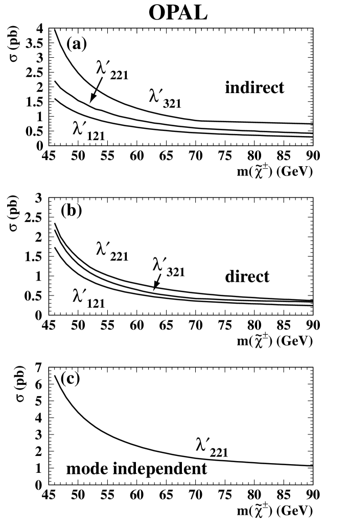
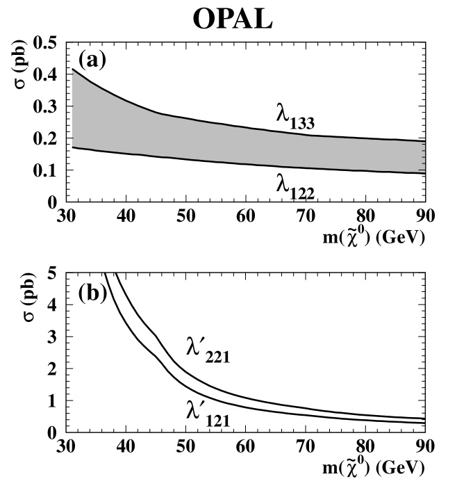
Figure 16 shows the upper limits on the cross-sections for the decay of a $\tilde{\chi}^{\pm}_{1}$ via $\lambda^{{}^{\prime}}$ for (a) the indirect decay and (b) the direct decay mode for any of the 27 $\lambda^{{}^{\prime}}$ couplings. Limits arising from any other coupling $\lambda^{{}^{\prime}}$ lie below the limit shown for the coupling with the same first index. Figure 16(c) shows the upper limits on the cross-sections independent of the decay mode. Limits arising from any other coupling $\lambda^{{}^{\prime}}_{ijk}$, with $i=1,2;j,k=1,2,3$ lie below the limit shown. The limits are not as good as for decays via couplings $\lambda$, since the signal looks more like the Standard Model processes, and lie between 0.3 and 1.8 pb for masses above 70 GeV.

7.3 Chargino Decays via $\lambda^{{}^{\prime\prime}}$

Figure 17 shows the upper limits on the cross-sections for the decay of a $\tilde{\chi}^{\pm}_{1}$ via $\lambda^{{}^{\prime\prime}}$ for (a) the indirect decay, (b) the direct decay mode, and (c) independent of the decay mode. Limits arising from any other coupling $\lambda^{{}^{\prime\prime}}$ lie below the limit shown. As for this case the decay of one chargino decaying directly and the other indirectly has been simulated, the mode independent limit is similar to the direct and indirect one. The limits lie between 1.0 and 1.8 pb for masses above 70 GeV.

7.4 Neutralino Decays

Figure 18 shows the upper limits on the cross-sections for the decay of a $\tilde{\chi}^{0}_{1}$. Limits arising from a decay via a coupling $\lambda$ lie between the two limits shown in (a). In (b) the upper limits for a decay via $\lambda^{{}^{\prime}}$ are shown. Limits arising from any other coupling $\lambda^{{}^{\prime}}$ lie below the limit shown for the coupling with the same first index.

8 Interpretation in the MSSM

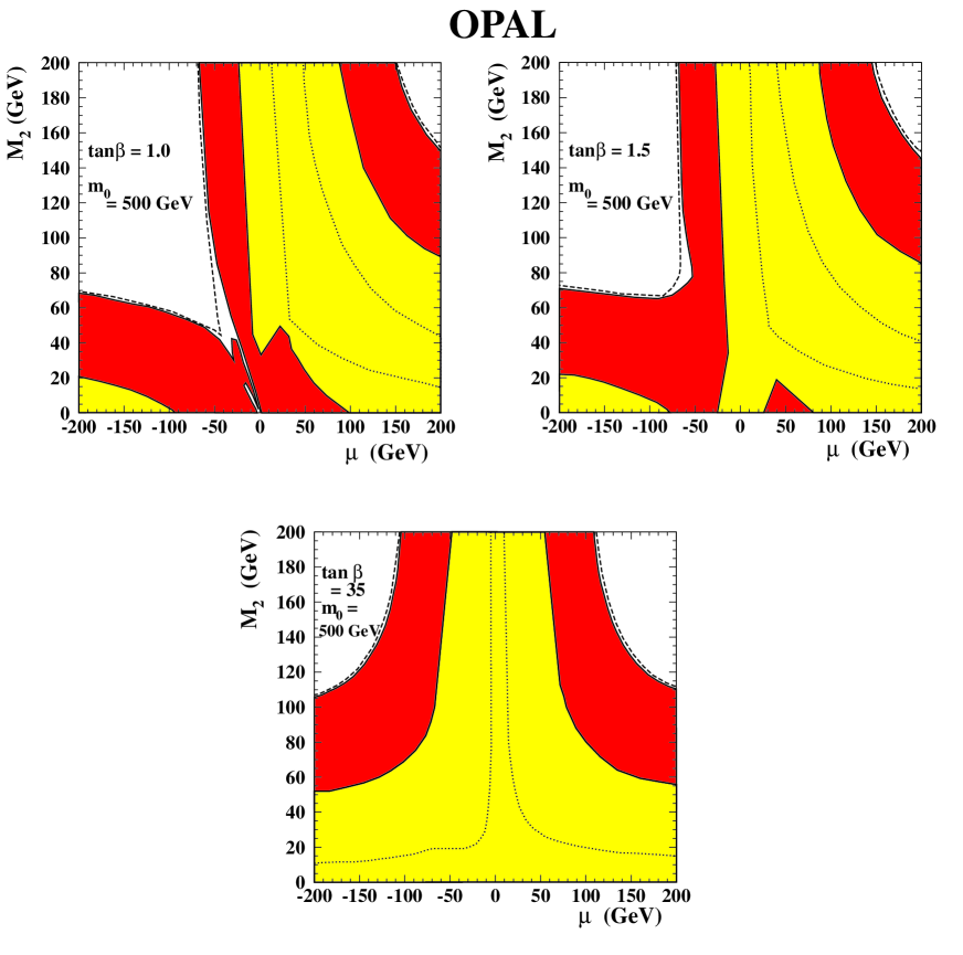
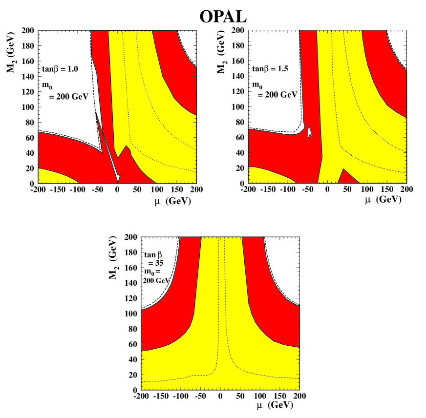
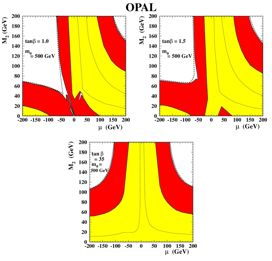
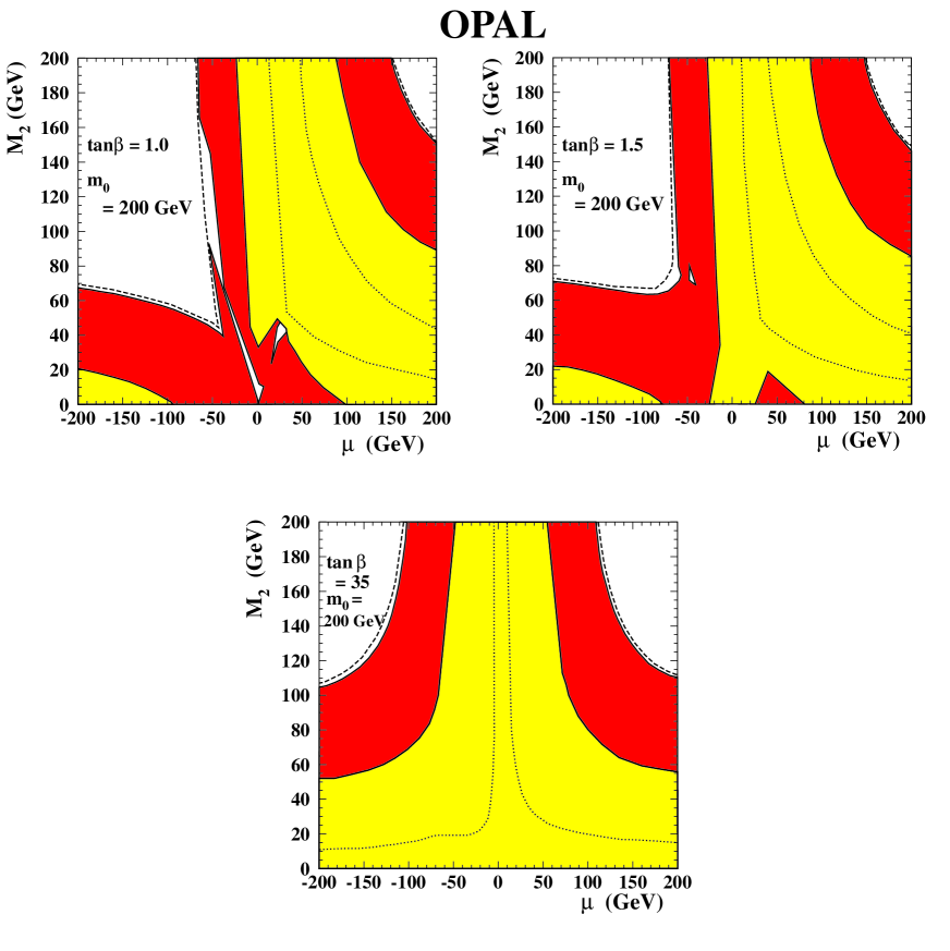
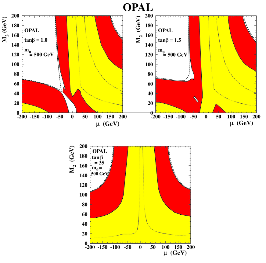
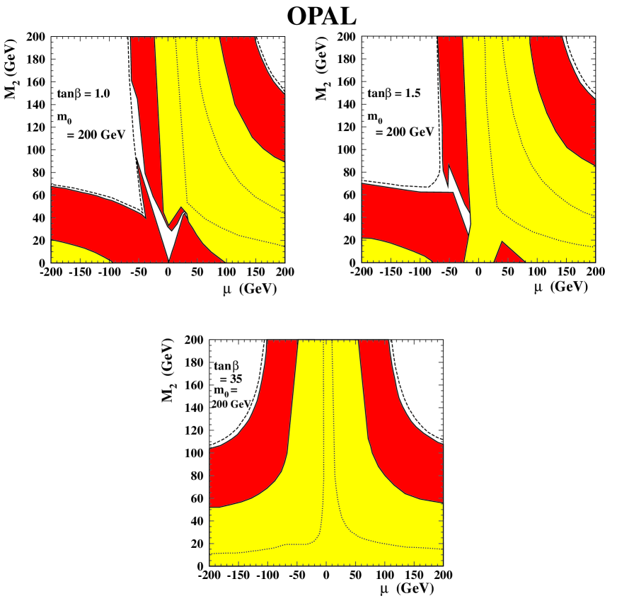
From the cross-section upper limits presented in Chapter 7, regions in the MSSM parameter space can be excluded. These regions are shown in Figures 19 to  24 in the ($M_{2}$, $\mu$) plane for $m_{0}$ = 500 GeV and 200 GeV and for $\tan\beta$ = 1.0, 1.5, and 35.0. The results are presented separately for decays with the $\lambda$, $\lambda^{{}^{\prime}}$, and $\lambda^{{}^{\prime\prime}}$couplings being different from zero.

The exclusion limits are determined by combining the following: the excluded cross-sections from the excess Z⁰ width [19], by comparing the measured and predicted width of the Z⁰ (light grey area); the cross-section upper limits from the pair production of $\tilde{\chi}^{\pm}_{1}$ and their decay via a $\lambda$-coupling (black area), using the worst limit and consequently making the excluded region independent of decay type. The production cross-section for $\tilde{\chi}^{0}_{1}$ pairs is so small that limits from the $\tilde{\chi}^{\pm}_{1}$ analyses are more precise than the $\tilde{\chi}^{0}_{1}$ limits everywhere. The regions excluded for $m_{0}$ = 500 GeV are also valid for $m_{0}>$ 500 GeV.

Although the Monte Carlo events have only been generated for $\Delta m=m(\tilde{\chi}^{\pm}_{1})-m(\tilde{\chi}^{0}_{1})>$5 GeV, the regions with $\Delta m<$5 GeV are excluded from the total Z⁰ width in the regions shown in the figures. Only for large values of $M_{2}$ ( $>$800 GeV) regions with $\Delta m<$5 GeV cannot be excluded. The area with $\Delta m<$5 GeV lies inside the two dotted lines in the figures.

For values of $\tan\beta$ smaller than 2, the branching ratio of $\tilde{\chi}^{\pm}_{1}\rightarrow W^{(*)}\tilde{\chi}^{0}_{2}$ with the subsequent decay of $\tilde{\chi}^{0}_{2}\rightarrow\tilde{\chi}^{0}_{1}\gamma$ can become as large as one for small $M_{2}$ and for $\mu$ negative and small. We have checked that our analyses are sensitive to these decays. For $\tan\beta\leq 2.0$ regions with the above decay exist, that cannot be excluded with the present data with the mode independent cross-section upper limit.

The regions excluded in the MSSM parameter space for exactly one coupling $\lambda$ not equal to zero are shown in Figures 19 and 20 independent of direct or indirect decay mode. The figures show that the excluded area is very close to the kinematic limit for $\tilde{\chi}^{\pm}_{1}$ pair production.

The regions excluded in the MSSM parameter space for exactly one coupling $\lambda^{{}^{\prime}}$ not equal to zero are shown in Figures 21 and 22 for the indirect decay. For large values of $\tan\beta$ the excluded region goes up to the kinematic limit, but for smaller values, unexcluded regions exist even for chargino masses as small as 45 GeV.

For one coupling $\lambda^{{}^{\prime\prime}}$ not equal to zero the regions excluded in the MSSM parameter space are shown in Figures 23 and 24 independent of the decay mode. Also here unexcluded regions exist for small values of $\tan\beta$.

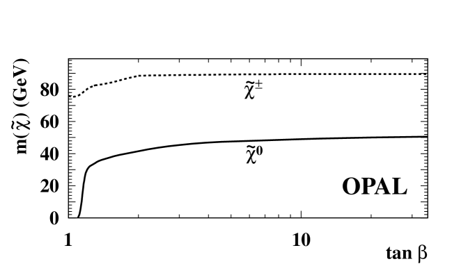
Each point in the MSSM parameter space corresponds to a $\tilde{\chi}^{\pm}_{1}$ and a $\tilde{\chi}^{0}_{1}$ mass pair. By excluding regions of this parameter space one can therefore also limit the allowed mass domains for these particles. The excluded masses for $\tilde{\chi}^{0}_{1}$ for a given $m_{0}$ depend on the value of $\tan\beta$ and are shown in Figure 25 for any coupling $\lambda$ greater than zero. Due to the small unexcluded regions in the MSSM parameter space for values of $\tan\beta\sim$1.0, no mass limit can be given for that region. For $\tan\beta>$1.2 the lower limit on the $\tilde{\chi}^{0}_{1}$ mass is 29 GeV for $m_{0}$ = 500 GeV, increasing up to 50 GeV for $\tan\beta>$20.

The limits for the $\tilde{\chi}^{\pm}_{1}$ depend much less on $\tan\beta$ than those of the $\tilde{\chi}^{0}_{1}$. For the $\tilde{\chi}^{\pm}_{1}$ a mass up to 76 GeV is excluded for any coupling $\lambda$  for any point in the MSSM parameter space, with $m_{0}$ = 500 GeV, under the assumption that it decays via a W^(∗).

Figure 15: 95% CL upper limits on cross-sections from the decay of a $\tilde{\chi}^{\pm}_{1}$ via a coupling $\lambda$, assuming a mass difference $\Delta m=m(\tilde{\chi}^{\pm}_{1})-m(\tilde{\chi}^{0}_{1})>5$ GeV. The cross-section limits are shown (a) for the indirect decay mode (b) for the direct decay mode and (c) independent of the decay mode. The cross-section limits for any coupling $\lambda$ lie below the limit for a decay via $\lambda_{133}$. For the (a) direct decay mode and the (b) indirect decay mode also the best cross-section limit, corresponding to $\lambda_{122}$, is shown.

Figure 16: 95% CL upper limits on cross-sections from (a) the indirect and (b) the direct decay and (c) independent of the decay mode of a $\tilde{\chi}^{\pm}_{1}$ via a coupling $\lambda^{{}^{\prime}}$. In (a) and (b) the excluded cross-sections for any coupling $\lambda^{{}^{\prime}}$ lie between the upper and lower curves. Also indicated are the couplings for which the best and the worst upper limits have been achieved. In (c) the upper limit is given for any coupling $\lambda^{{}^{\prime}}_{ijk}$ with $i=1,2$.

Figure 17: 95% CL upper limits on cross-sections from the decay of a $\tilde{\chi}^{\pm}_{1}$ via a coupling $\lambda^{{}^{\prime\prime}}$, assuming a mass difference $\Delta m=m(\tilde{\chi}^{\pm}_{1})-m(\tilde{\chi}^{0}_{1})>5$ GeV. The cross-section limits are shown (a) for the indirect decay mode (b) for the direct decay mode and (c) independent of the decay mode. The cross-section limits for any coupling $\lambda^{{}^{\prime\prime}}$ lie below the limit for a decay via $\lambda^{{}^{\prime\prime}}_{122}$.

Figure 18: 95% CL upper limits on cross-sections from the direct decay of a $\tilde{\chi}^{0}_{1}$ via (a) a coupling $\lambda$ and (b) a coupling $\lambda^{{}^{\prime}}$. The cross-section limits for any coupling $\lambda$ lie in the gray zone between the two limits shown. The limit for $\lambda^{{}^{\prime}}_{321}$ lies on top of that for $\lambda^{{}^{\prime}}_{121}$. Limits arising from any other coupling $\lambda^{{}^{\prime}}$ lie below the limit shown for the coupling with the same first index.

Figure 19: Excluded region in the M₂ – $\mu$ plane from the decay of $\tilde{\chi}^{\pm}_{1}$, for $\lambda$ $\neq 0$, $\lambda^{{}^{\prime}}$=$\lambda^{{}^{\prime\prime}}$=0, for m${}_{0}=500$ GeV. The dark area shows the points excluded by the LEP2 searches and the light area the points excluded from the Z⁰ width. The dashed line shows the kinematic limit for $\sqrt{s}=183$ GeV, and the dotted line shows the area with $\Delta m<5$ GeV.

Figure 20: Excluded region in the M₂ – $\mu$ plane from the decay of $\tilde{\chi}^{\pm}_{1}$ for $\lambda$ $\neq 0$, $\lambda^{{}^{\prime}}$=$\lambda^{{}^{\prime\prime}}$=0, for m${}_{0}=200$ GeV. The dark area shows the points excluded by the LEP2 searches and the light area the points excluded from the Z⁰ width. The dashed line shows the kinematic limit for $\sqrt{s}=183$ GeV, and the dotted line shows the area with $\Delta m<5$ GeV.

Figure 21: Excluded region in the M₂ – $\mu$ plane from the indirect decay of $\tilde{\chi}^{\pm}_{1}$ for $\lambda^{{}^{\prime}}$ $\neq 0$, $\lambda$=$\lambda^{{}^{\prime\prime}}$=0, for m${}_{0}=500$ GeV. The dark area shows the points excluded by the LEP2 searches and the light area the points excluded from the Z⁰ width. The dashed line shows the kinematic limit for $\sqrt{s}=183$ GeV, and the dotted line shows the area with $\Delta$ m $<$ 5 GeV

Figure 22: Excluded region in the M₂ – $\mu$ plane from the indirect decay of $\tilde{\chi}^{\pm}_{1}$ for $\lambda^{{}^{\prime}}$ $\neq 0$, $\lambda$=$\lambda^{{}^{\prime\prime}}$=0, for m${}_{0}=200$ GeV. The dark area shows the points excluded by the LEP2 searches and the light area the points excluded from the Z⁰ width. The dashed line shows the kinematic limit for $\sqrt{s}=183$ GeV, and the dotted line shows the area with $\Delta m<5$ GeV.

Figure 23: Excluded region in the M₂ – $\mu$ plane from the decay of $\tilde{\chi}^{\pm}_{1}$ for $\lambda^{{}^{\prime\prime}}$ $\neq 0$, $\lambda$=$\lambda^{{}^{\prime}}$=0, for m${}_{0}=500$ GeV. The dark area shows the points excluded by the LEP2 searches and the light area the points excluded from the Z⁰ width. The dashed line shows the kinematic limit for $\sqrt{s}=183$ GeV, and the dotted line shows the area with $\Delta m<5$ GeV.

Figure 24: Excluded region in the M₂ – $\mu$ plane from the decay of $\tilde{\chi}^{\pm}_{1}$ for $\lambda^{{}^{\prime\prime}}$ $\neq 0$, $\lambda$=$\lambda^{{}^{\prime}}$=0, for m${}_{0}=200$ GeV. The dark area shows the points excluded by the LEP2 searches and the light area the points excluded from the Z⁰ width. The dashed line shows the kinematic limit for $\sqrt{s}=183$ GeV, and the dotted line shows the area with $\Delta m<5$ GeV.

Figure 25: Excluded masses for $\tilde{\chi}^{0}_{1}$ (solid line) and $\tilde{\chi}^{\pm}_{1}$ (dashed line) as a function of $\tan\beta$ for m${}_{0}=500$ GeV for any coupling $\lambda$. The exclusion limits for the $\tilde{\chi}^{0}_{1}$ do not result from the direct search for $\tilde{\chi}^{0}_{1}$ decays but from the excluded CMSSM parameter space from the $\tilde{\chi}^{\pm}_{1}$ searches.

9 Conclusions

We have been searching for $R$-parity violating decays of charginos and neutralinos via the Yukawa couplings $\lambda$, $\lambda^{{}^{\prime}}$, and $\lambda^{{}^{\prime\prime}}$. Analyses have been presented for a large number of final states arising from these decays, varying from two leptons up to more than four jets. We have not observed any excess of events. Limits on the cross section times branching ratio, ranging from 0.08 pb up to several pb, have been presented separately for all these topologies. From these, upper limits on the pair production cross-section of $\tilde{\chi}^{\pm}_{1}$ and $\tilde{\chi}^{0}_{1}$ are obtained and presented separately for $\lambda$, $\lambda^{{}^{\prime}}$, and $\lambda^{{}^{\prime\prime}}$for direct, indirect and mixed decay modes. For $\lambda$ and $\lambda^{{}^{\prime\prime}}$  limits have also been presented which are valid independently of whether the decays are direct or indirect.

Finally, the limits are interpreted in the framework of the MSSM. Most of the kinematically accessible regions in the $M_{2}-\mu$ plane for $m_{0}\geq$ 500 GeV have been excluded. Lower mass limits, of 76 GeV for $\tilde{\chi}^{\pm}_{1}$ at $m_{0}$ = 500 GeV and $\tan\beta\geq$1.0, and 29 GeV for $\tilde{\chi}^{0}_{1}$ at $m_{0}$ = 500 GeV and $\tan\beta\geq$1.2, have been obtained independently of which of the couplings $\lambda$, $\lambda^{{}^{\prime}}$, and $\lambda^{{}^{\prime\prime}}$  is assumed to be different from zero. All the limits are valid at the 95% confidence level, for couplings larger than 10^-5.

Acknowledgements

We particularly wish to thank the SL Division for the efficient operation of the LEP accelerator at all energies and for their continuing close cooperation with our experimental group. We thank our colleagues from CEA, DAPNIA/SPP, CE-Saclay for their efforts over the years on the time-of-flight and trigger systems which we continue to use. In addition to the support staff at our own institutions we are pleased to acknowledge the
Department of Energy, USA,
National Science Foundation, USA,
Particle Physics and Astronomy Research Council, UK,
Natural Sciences and Engineering Research Council, Canada,
Israel Science Foundation, administered by the Israel Academy of Science and Humanities,
Minerva Gesellschaft,
Benoziyo Center for High Energy Physics,
Japanese Ministry of Education, Science and Culture (the Monbusho) and a grant under the Monbusho International Science Research Program,
Japanese Society for the Promotion of Science (JSPS),
German Israeli Bi-national Science Foundation (GIF),
Bundesministerium für Bildung, Wissenschaft, Forschung und Technologie, Germany,
National Research Council of Canada,
Research Corporation, USA,
Hungarian Foundation for Scientific Research, OTKA T-016660, T023793 and OTKA F-023259.

References

-
[1]
H. P. Nilles, Phys. Rep. 110 (1984) 1;
H. E. Haber and G. L. Kane, Phys. Rep. 117 (1985) 75. - [2] I. Hinchliffe, T. Kaeding, Phys. Rev. D47 (1993) 279.
- [3] A.Y. Smirnow, F. Vissani, Phys. Lett. B380 (1996) 317.
- [4] G. Bhattacharyya, “A Brief Review of R-Parity Violating Couplings”, presented at the workshop on Physics Beyond the Standard Model: Beyond the Desert: Accelerator and Nonaccelerator Approaches, Tegernsee, Germany, 8-14 Jun 1997 (hep-ph/9709395).
- [5] ALEPH Collab., R. Barate et al., Euro. Phys. J. C4 (1998) 433.
- [6] OPAL Collab., K. Ackerstaff et al., Euro. Phys. J. C6 (1998) 1.
[7]
A. Bartl, H. Fraas and W. Majerotto, Z. Phys. C30 (1986) 441;
A. Bartl, H. Fraas and W. Majerotto, Z. Phys. C41 (1988) 475;
A. Bartl, H. Fraas, W. Majerotto and B. Mösslacher, Z. Phys. C55 (1992) 257. -
[8]
M. Chen, C. Dionisi, M. Martinez and X. Tata, Phys. Rep. 159 (1988) 201;
J. L. Feng and M. J. Strassler, Phys. Rev. D51 (1995) 4661. -
[9]
A. Bartl, H. Fraas and W. Majerotto, Nucl. Phys. B278 (1986) 1;
S. Ambrosanio and B. Mele, Phys. Rev. D52 (1995) 3900. - [10] M. Carena, J.R. Espinosa, M. Quiros and C.E.M. Wagner, Phys. Lett. 355B (1995) 209.
[11]
T. Sjöstrand and M. Bengtsson,
Comp. Phys. Comm. 43 (1987) 367;
“PYTHIA 5.7 and JETSET 7.4, Physics and Manual”, CERN-TH. 7112/93 (revised August 1995);
T. Sjöstrand, Comp. Phys. Comm. 82 (1994) 74. - [12] H. Dreiner, S. Lola, P. Morawitz, Phys. Lett. B389 (1996) 62.
- [13] H. Dreiner, P. Morawitz, Nucl. Phys. B428 (1994) 31.
- [14] S. Dawson, Nucl. Phys. B261 (1985) 297.
- [15] S. Dimopoulus and L.J. Hall, Phys. Lett. B207 (1987) 210.
- [16] OPAL Collaboration, K. Ackerstaff et al., “Search for Chargino and Neutralino Production at = 181 – 184 GeV at LEP”, CERN-EP/98-136, submitted to Euro. Phys. J. C.
- [17] J. Allison et al., Nucl. Instr. Meth. A317 (1992) 47.
- [18] S. Katsanevas and S. Melachroinos, in “Physics at LEP2”, eds. G. Altarelli, T. Sjöstrand and F. Zwirner, CERN 96–01, vol. 2, p. 328 (1996).
- [19] Particle Data Group, Phys. Rev. D54 (1996) 1.
- [20] OPAL Collab., K. Ackerstaff et al., Euro. Phys. J. C4 (1998) 47.
[21]
S. Jadach, W. Placzek and B.F.L. Ward, UTHEP/95-1001 (unpublished);
S. Jadach et al., in “Physics at LEP2”, eds. G. Altarelli, T. Sjöstrand and F. Zwirner, CERN 96–01, vol.2, p. 229 (1996);
S. Jadach, W. Placzek and B.F.L. Ward, Phys. Lett. B390 (1997) 298. - [22] S. Jadach, B.F.L. Ward and Z. Wa̧s, Comp. Phys. Comm. 79 (1994) 503.
[23]
R. Engel and J. Ranft, Phys. Rev. D54 (1996) 4244;
R. Engel, Z. Phys. C66 (1995) 203. - [24] G. Marchesini et al., Comp. Phys. Comm. 67 (1992) 465.
[25]
R. Bhattacharya, J. Smith and G. Grammer, Phys. Rev. D15 (1977) 3267;
J. Smith, J.A.M. Vermaseren and G. Grammer, Phys. Rev. D15 (1977) 3280. - [26] J.Fujimoto et al., Comp. Phys. Comm. 100 (1997) 128.
[27]
OPAL Collab., K. Ahmet et al., Nucl. Instr. Meth. A305 (1991) 275;
S. Anderson et al., Nucl. Instr. Meth. A403 (1998) 326. - [28] B.E. Anderson et al., IEEE Transactions on Nuclear Science 41 (1994) 845.
- [29] OPAL Collab., R. Akers et al., Z. Phys. C61 (1994) 19.
- [30] OPAL Collab., M.Z. Akrawy et al., Phys. Lett. B253 (1991) 511.
- [31] OPAL Collab., K. Ackerstaff et al., Euro. Phys. J. C2 (1998) 213.
- [32] OPAL Collab., K. Ackerstaff et al., Phys. Lett. B396 (1997) 301.
- [33] OPAL Collab., R. Akers et al., Phys. Lett. B327 (1994) 411.
- [34] OPAL Collab., R. Akers et al., Z. Phys. C60 (1993) 199.
- [35] OPAL Collab., P.D. Acton et al., Z. Phys. C60 (1993) 19.
- [36] OPAL Collab., G. Alexander et al., Z. Phys. C70 (1996) 357.
- [37] OPAL Collab., K. Ackerstaff et al., Phys. Lett. B389 (1996) 416.
- [38] R. D. Cousins and V. L. Highland, Nucl. Instr. Meth. A320 (1992) 331.
[39]
N. Brown and W.J. Stirling, Phys. Lett. B252 (1990) 657;
S. Bethke, Z. Kunszt, D. Soper and W.J. Stirling, Nucl. Phys. B370 (1992) 310;
S. Catani et al., Phys. Lett. B269 (1991) 432;
N. Brown and W.J. Stirling, Z. Phys. C53 (1992) 629. - [40] OPAL Collaboration, K. Ackerstaff et al., Euro. Phys. J. C1 (1998) 425.
- [41] OPAL Collaboration, K. Ackerstaff et al., Phys. Lett. B391 (1997) 221.
- [42] OPAL Collaboration, K. Ackerstaff et al., Euro. Phys. J. C2 (1998) 441.
- [43] OPAL Collaboration, K. Ackerstaff et al., “Search for Higgs Bosons in e+e- Collisions at =183 GeV”, CERN-EP/98-173, submitted to Euro. Phys. J. C.
- [44] OPAL Collaboration, K. Ackerstaff et al., Euro. Phys. J. C5 (1998) 19.
- [45] OPAL Collaboration, G. Alexander et al., Phys. Lett. B376 (1996) 232.
- [46] R.K. Ellis, D.A. Ross and A.E. Terrano, Nucl. Phys. B178 (1981) 421.
[47]
A.G. Frodesen, O. Skeggestad, and H. Tofte,
“Probability and Statistics in
Particle Physics”, Universitetsforlaget, 1979, ISBN 82-00-01-01906-3;
S.L. Meyer, Data Analysis for Scientists and Engineers, John Wiley and Sons, 1975, ISBN 0-471-59995-6.