JET PHYSICS AT LEP
AND
WORLD SUMMARY OF aaaPresented
at the Int. Symp. on Radiative Corrections, Barcelona, Sept. 8-12,
1998.
Recent results on jet physics and tests of QCD from hadronic final states in annihilation at PETRA and at LEP are reviewed, with special emphasis on hadronic event shapes, charged particle production rates, properties of quark and gluon jets and determinations of . The data in the entire energy range from PETRA to LEP-2 are in broad agreement with the QCD predictions. The world summary of measurements of is updated and a detailed discussion of various methods to determine the overall error of is presented. The new world average is . The size of the error depends on the treatment of correlated uncertainties.
1 Annihilation Data
Over the past few years, a large amount of annihilation data in the c. m. energy range from Q 10 to 189 GeV was accumulated at the CESR, PETRA, PEP, Tristan, LEP and SLC accelerators. The large data samples at LEP-1, which amount to about 4 million hadronic events around the resonance for each of the four LEP experiments, and the most recent data at the highest energies of LEP-2 (a few thousand events per experiment), together with reanalysed PETRA data at lower c.m. energies (about 50.000 hadronic events), provide powerful tools for precise tests of perturbative QCD.
At energies below or at the resonance, respectively at PETRA and at LEP-1, the study of annihilation events is rather “easy” and straight forward: apart from two-photon processes, the energy and quantum numbers of the hard scattering are well defined and different processes can be identified and selected with only very little backgrounds or biases. At LEP-2, i.e. at energies above the pole, the situation is more complicated:
-
•
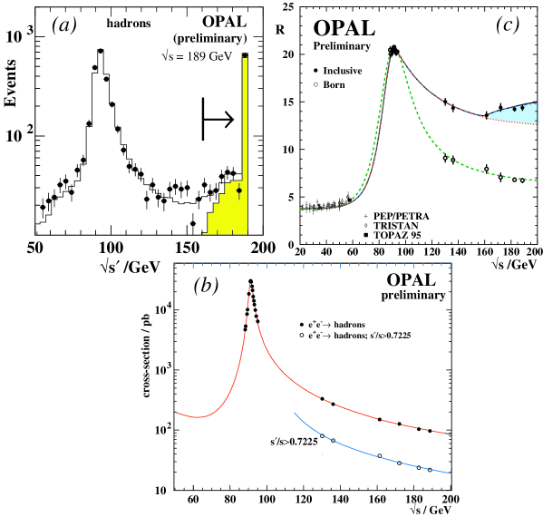
The annihilation cross section is orders of magnitude lower than at the pole; see Figure 1b.
-
•
Initial state photon radiation reduces the available energy of the hadronic c.m. system, , see Figure 1a, and causes, together with the resonant cross section around the mass, a large “return-to-the-Z” effect. Radiative events can be suppressed requiring a minimum reconstructed ratio of and other kinematic constraints.
-
•
Other processes like and emerge above the respective energy thresholds, see the shaded area in Figure 1c, causing a certain irreducable background for QCD studies.
In the following sections, recent QCD tests from LEP-1 ( GeV; Section 2), from LEP-2 ( GeV to 189 GeV; Section 3) and from a combination of PETRA and LEP data ( GeV to 172 GeV; Section 4) are presented. The world summary of is updated in Section 5.
2 QCD Tests at LEP-1
2.1 from Event Shapes using Optimised QCD
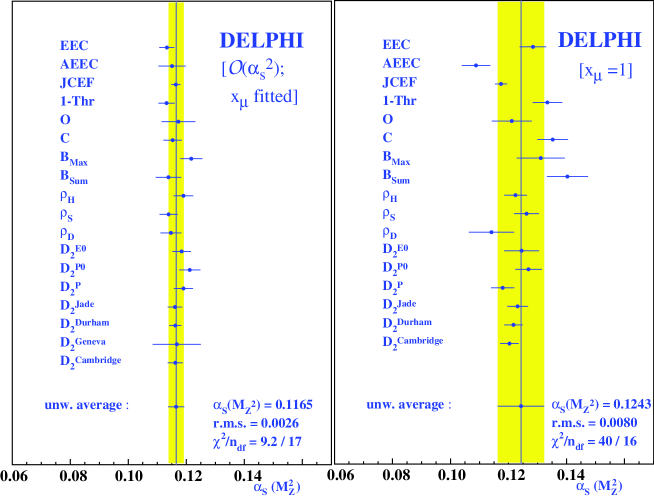
The DELPHI collaboration contributed a new measurement of from oriented event shape distributions at LEP-1 . 17 different event shape observables are measured as a function of the polar angle of the thrust axis, and is determined from fits to QCD calculations. As already reported earlier , good agreement between theory and data can be obtained if both and the renormalisation scale are determined simultaneously; see Figure 2.
With optimised renormalisation scales and allowing for scale uncertainties between and , consistent results of emerge, leading to a combined average of . Both the average and the error, which includes theoretical uncertainties from scale changes as given above, are smaller than those obtained from resummed QCD fits. This is basically due to the choice of the averaging procedure and error definition.bbb Note that, for instance, a previous study based on 13 observables and using a different procedure to average results and determine the overall error obtained which, if the same procedure as used in the DELPHI analysis is applied, converts to . The broad consistency between data and optimised QCD justifies this procedure and suggests to reconsider optimised fixed order perturbation theory as an alternative to resummation which was preferred in the past.
2.2 Differences between Quark- and Gluon-Jets
Differences between quark- and gluon-jets were studied quite intensively during the past few years. The aim is to test the basic QCD prediction that hadrons coming from gluon jets should exhibit a softer energy spectrum and a wider transverse momentum distribution than those originating from quark jets, due to the larger colour charge of the gluon. In particular, the ratio of the average multiplicities of hadrons in gluon jets and in quark jets should, for infinite jet energies and in leading order QCD, be .
Experimental procedures to separate quark- from gluon-jets are usually based on vertex tagging of primary b-quark decays. In short, 3-jet like events are selected in which one of the two lower energetic jets is tagged as a b-quark, while the other low energy jet is then taken to be the gluon jet. From first analyses of this type it was found that, after correction for misidentified jets, . No QCD calculation for this particular type of analysis exists, such that a direct comparison of this result with theory is not possible.
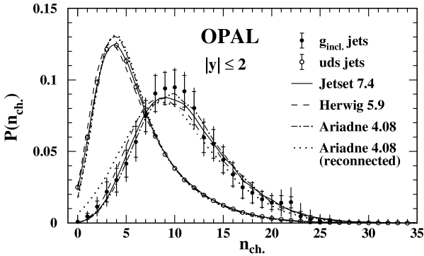
Theoretical predictions only exist for colour singlet and final states, where however the latter state is not experimentally accessible. In order to perform an analysis closer to theory, OPAL followed a new strategy in which events with a high-energetic gluon-jet recoiling against a (vertex-tagged) system were selected. Such events are relatively rare, leading to about 550 selected gluon jets from OPAL’s LEP-1 data sample.
A comparison of the charged hadron multiplicity distribution of such gluon hemispheres with those of ordinary light quark event hemispheres is shown in Figure 3, where a significant difference between quark- and gluon-jets is seen. For a central rapidity range, the hadron multiplicity ratio is found to be ; the remaining difference to the QCD expectation of 2.25 is likely to be explained by finite jet energy effects.
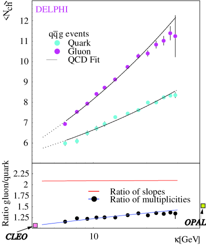
DELPHI has studied the scale dependence of particle multiplicities in quark- and gluon-jets . Here, gluon-jets and light quark-jets are (anti-)tagged in 3-jet events, and a jet energy scale of , where is the angle between the two lowest energetic jets, is defined. The charged hadron multiplicities for quark- and gluon-jets, as a function of , are diplayed in Figure 4. Also shown is the ratio of multiplicities and the ratio of slopes; the latter being close to the QCD prediction of 2.25.
From these measurements DELPHI determines the ratio to be which is in good agreement with QCD, and in particular with the expected colour charge of the gluon.
3 QCD Tests at LEP-2
3.1 Hadronic Event Shapes and Running of
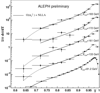
At each new energy point of LEP-2, all four LEP experiments have extensively studied hadronic event shape distributions and compared the new measurements with the predictions of QCD Monte Carlo models, as well as with analytic QCD calculations. In all cases, up to and including the most recent data at GeV, good agreement of data and theory was found, and no significant deviation from the standard expectation was seen. As an example, Figure 5 shows the thrust-distributions measured by ALEPH at LEP-1 and at four energy points of LEP-2, together with a fit to resummed QCD calculations which is in good agreement with the data at all energies.
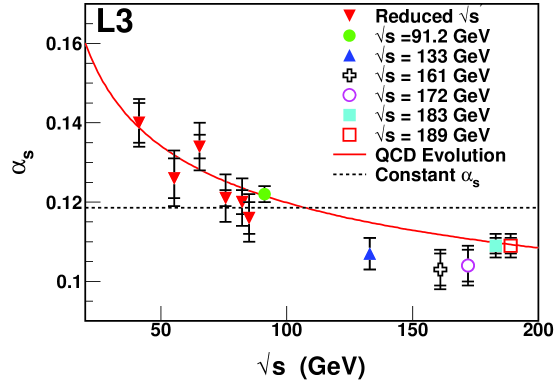
The L3 collaboration has summarised their measurements of from various event shape distributions, at LEP-1, at all LEP-2 energy points, and at hadronic c.m. energies below the pole, from an analysis of radiative events recorded at LEP-1. The data, which are displayed in Figure 6, are in very good agreement with the QCD prediction of a running coupling .
3.2 Energy Dependence of Charged Particle Production
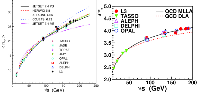
The energy dependence of particle production was, similarly as hadronic event shapes, continuously monitored by all LEP experiments. The variation of such observables with energy is found to be in good agreement with QCD predictions, and also with the “standard” QCD plus hadronisation models. The energy dependence of the average charged hadron multiplicity and of the peak position of the distribution () are shown in Figure 7.
4 Power Corrections and Energy Dependence of Event Shapes
The energy dependence of mean values of event shape observables can be parametrised by the perturbative QCD prediction plus a term including the improved two-loop calculations (the “Milan factor”) of power-suppressed 1/Q non-perturbative contributions , the so-called “power corrections”. The latter contains the moment of an effective coupling below an infrared scale , which is expected to be universal for all applicable event shape observables.
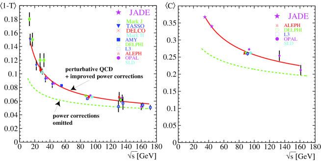
A compilation of available data on the mean value of (1-thrust) and of the C-parameter is shown in Figure 8, which is taken from a recent re-analysis of JADE data at PETRA energies . Perturbative QCD plus power corrections is found to give a very good description of the data, with as determined from these data. However, universality of is only found to be satisfied at a level of 30%.
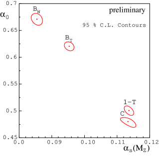
For differential event shape distributions, the power corrections are simply a shift of the perturbative () spectra, and these were also studied in a wide c.m. energy range, including the most recent PETRA and LEP data for a total of four event shape observables . A fit to these data, with and as free parameters for each observable, leads to the results displayed in Figure 9. Agreement in both and is obtained, to a good level of accuracy, for two of the observables. However, the jet broadening parameters and deviate significantly in both and .
Most recently, the reason for these deviations was identified and traced to the theoretical predictions ; a cure of this problem should soon be available.
5 World Summary of
Significant determinations of the strong coupling strength, , remain to be a demanding and interesting topic in experimental as well as theoretical study projects in high energy physics. In the following subsections, previous summaries of measurements will be updated and a new world average will be determined. Instead of a complete reference to all available measurements, only the newest results are briefly introduced, and more emphasis is spent on a detailed discussion of the overall uncertainty of , .
5.1 Updates and New Results
The results of all significant determinations of , i.e. of all those which are based on QCD calculations which are complete - at least - to next-to-leading order perturbation theory, are summarised in Table 2. The following entries were added or updated since summer 1997 (underlined in Table 2):
-
•
The most recent determination of from the GLS sum rules, based on new data from scattering is included, replacing the previous result from Chyla and Kataev .
-
•
New measurements of from high statistics studies of vector and axial-vector spectral functions of hadronic -decays are available from ALEPH and OPAL . As the most complete and precise studies of decays to date, these results are combined and taken to replace earlier results .
-
•
H1 has contributed new determinations of from (2+1)-jet event rates at HERA , replacing a previous measurement . A combination of these new results with a former one from ZEUS is updated in Table 2.
-
•
A new determination of from -decays replaces earlier results .
-
•
A recent determination of from the total hadronic cross section measured by CLEO at GeV is added.
-
•
Determinations of from JADE data, at and 44 GeV, were updated by the inclusion of another observable, the C-parameter.
-
•
from the most recent LEP result on was updated (these results are still preliminary).
-
•
LEP results on from event shapes measured at and 189 GeV are combined and added to the list (some of these results are still preliminary).
Further interesting and recent developments are a QCD analysis of neutrino deep inelastic scattering data for , in next-next-to-leading order of perturbation theory (NNLO) , resulting in , and a reanalysis of muon deep inelastic scattering data , resulting in . Both these results are subject to further completion and verification; they are therefore considered to be preliminary and are not included in this summary.
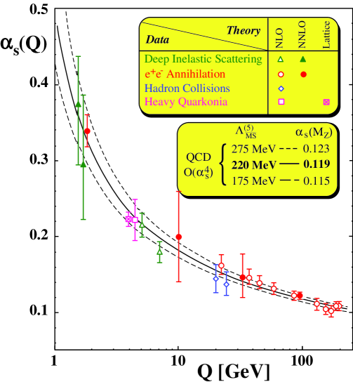
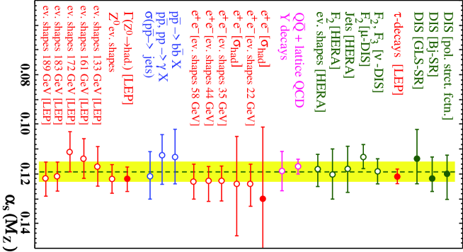
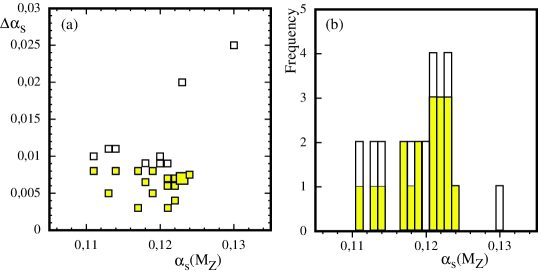
The results for , given in the row of Table 2, are presented in Fig. 10. These results are evolved from the energy scale , i.e. the typical energy scale of the hard scattering process under study, to the reference energy scale , by using the QCD 4-loop beta-function with 3-loop matching at quark pole masses GeV and GeV , resulting in the values of given in the row of Table 1. These values of are displayed in Fig. 11. The distribution of all results is shown in a scatter plot of versus its quoted error, , and in a frequency distribution of (Figure 12).
The world average value of and its overall uncertainty as well as the corresponding QCD curves shown in Figs. 10 and 11 will be discussed in the following section.
5.2 World Average and Overall Uncertainty of
In order to average the results of , a weigthed mean of the quoted central values is calculated, for all results as well as for subsamples as listed in Table 1. The weight of a measurement is taken to be the inverse of the square of its total error.
The central value does not depend on details of the weighting method; no significant differences are found if, for instance, the simple and unweighted mean is taken. Also, and more important, there are no significant differences between values of calculated from different subsamples of the data: the averages from the high- and the low-energy data as well as those from annihilation, from DIS and from colliders agree well with each other and with the overall average of = 0.119, within the respective errors (irrespective of how those errors are defined; see the discussion below).
While the central value of is remarkably stable and well defined, the determination of its overall uncertainty, , depends very much on the detailed definition of what this uncertainty should be, and how it should be calculated. There are several reasons for this situation:
The errors of most results are dominated by theoretical uncertainties, which are estimated using a variety of different methods and definitions. The significance of these non-gaussian errors is largely unknown. Furthermore, there are large correlations between different results, due to common theoretical uncertainties, as e.g. in the case of various event shape measurements in annihilations. Nothing is known, however, about possible correlations between determinations from different processes, such as DIS and annihilations, or between different procedures and observables used within the same class of processes.
Therefore, in the past, the value of was often “guess-timated”, and/or a variety of mathematical methods was applied to obtain a reasonable estimate. Some of these methods will be applied and discussed in the following; the results are summarised in Table 1:
| uncorrel. | simple rms | rms box | opt. corr. | overall | ||
|---|---|---|---|---|---|---|
| sample (entries) | correl. | |||||
| all (27) | 0.1193 | 0.0012 | 0.0044 | 0.0059 | 0.0049 | 0.71 |
| (18) | 0.1193 | 0.0013 | 0.0038 | 0.0052 | 0.0042 | 0.64 |
| (7) | 0.1190 | 0.0016 | 0.0033 | 0.0041 | 0.0030 | 0.49 |
| (2) | 0.1190 | 0.0021 | 0.0028 | 0.0028 | 0.0022 | 0.11 |
| only (15) | 0.1210 | 0.0016 | 0.0045 | 0.0059 | 0.0052 | 0.77 |
| only DIS (8) | 0.1175 | 0.0025 | 0.0029 | 0.0053 | 0.0061 | 0.80 |
| only (3) | 0.1156 | 0.0057 | 0.0053 | 0.0072 | 0.0088 | 0.69 |
| GeV (9) | 0.1184 | 0.0016 | 0.0029 | 0.0045 | 0.0038 | 0.69 |
| GeV (14) | 0.1199 | 0.0020 | 0.0047 | 0.0062 | 0.0060 | 0.69 |
-
•
For illustrational purposes only, an overall error is calculated assuming that all measurements are entirely uncorrelated and all quoted errors are gaussian. The results are displayed in the column of Table 1.
-
•
The simple, unweigthed of the mean value of all measurements is calculated and shown in the column, labelled “simple rms”.
-
•
Assuming that each result of has a rectangular-shaped rather than a gaussian probability distribution, all resulting weights (the inverse of the square of the total error) are summed up in a histogram, and the resulting of that distribution is quoted as “rms box” .
-
•
A correlated error is calculated from the error covariance matrix, assuming an overall correlation factor between all measurements. The correlation factor is adjusted such that the total is one per degree of freedom . The resulting errors and correlation factors are given in the last two columns of Table 1 (labelled “optimised correlation”).
All of the methods defined above have certain advantages but also obey inherent problems. The “simple rms” indicates the scatter of all results around their common mean, but does not depend on the individual errors quoted for each measurement. The “box rms”, which takes account of the individual errors and of their non-gaussian nature, was criticised to be too conservative an estimate of the overall uncertainty of . The “optimised correlation” method is closest to a mathematically appropriate treatment of correlated errors, however - in the absence of a detailed knowledge of these correlations - over-simplifies by the (unphysical ?) assumption of one overall correlation factor, identical to all pairs of measurements. Moreover, the calculated from the covariance matrix does not have, if correlations are present, the same mathematical and propabilistic meaning as in the case of uncorrelated data. In the extreme, may even be negative.
With these reservations in mind, all three methods do provide some estimate of . Apart from systematic differences in the size of , they all depend on the significance of the data included in the averaging process: in all cases, is largest if all data are included, and tend to smaller values if the averaging is restricted to results with errors , i.e. if only the most significant results are used to calculate and .
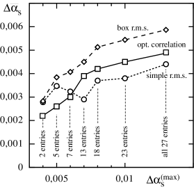
This can be seen from Table 1, where and are also shown for three subsets of data with 0.008, 0.006 and 0.004. The decrease of as a function of is graphically shown in Figure 13. All three estimates of , the “simple rms”, the “box rms” and the “optimised correlation”, decrease from intial values of 0.004 … 0.006, if all results are taken into account, to about 0.003 if only the most “precise” results are included. Only at the very extreme, taking the two results with the smallest quoted errors, the “optimised correlation” method yields an overall error of less than 0.003. Note that, despite the dependence of on the choice of , the overall average does depend on this selection!
On first sight it seems logical to restrict the determination of , and especially of , to the most significant data, if inclusion of insignificant measurements enlarges . Taken to the extreme, one may even be tempted to quote the one result which carries the smallest quoted error as the final world average value of and . However, the errors on estimated in individual studies are, in general, lower limits because unknown and additional systematic effects can only increase the total error. Small systematic errors of single measurements may well be due to ignorance, over-optimism and/or neglection of certain error sources, which may be difficult to judge. Indeed, the errors of the two results with the smallest errors quoted, from -decays and from heavy quark bound states using lattice gauge theory, were often criticised as being overly optimistic.
In this sense, averaging over a number of well understood and commonly accepted measurements of reasonable precision is a safe basis to estimate and . While there is still a large degree of flexibility to choose the final data set and the procedure to estimate , the choice to select results with and to determine using the “optimised correlation” method seems reasonable and to be neither overly optimistic nor pessimistic. The final world average of is therefore quoted to be, c.f. Table 1 and Figure 13,
The central values of 19 out of the 27 measurements listed in Table 2, or equivalently 70%, are inside this error range of , thus being compatible with the expectation of a “one standard deviation” interval.
If the result of which is based on lattice gauge theory is omitted in the averaging process, and increase to . The same is true if the result of the reanalysis of muon deep inelastic scattering data is usedccc The increase of is due to an artifact of the “optimised correlation” method which may increase the overall correlation factor (and thus, the overall error) if individual measurements are closer to their common mean. instead of the one listed in Table 2.
Note that the value of = 0.004 is a factor of two larger than the one quoted in the latest edition of the Review of Particle Physics . The smaller value of 0.002 quoted there corresponds to a (slighly enlarged) r.m.s. assuming all measurements to be totally uncorrelated; an assumption which seems, in view of the results discussed above, unrealistic.
Acknowledgments
I am grateful to W. Bernreuther, to O. Biebel, to S. Catani, to A. Kataev and to Yu. Dokshitzer for helpful discussions.
References
References
- [1] DELPHI Collaboration, DELPHI 98-84 CONF 152.
- [2] S. Bethke, Z. Phys. C43 (1989) 331.
- [3] DELPHI Collaboration, P. Abreu et al., Z. Phys. C54 (1992) 55 .
- [4] OPAL Collaboration, P.D. Acton et al., Z. Phys. C55 (1992) 1.
- [5] OPAL Collaboration, P. Acton et al., Z. Phys. C58 (1993) 387.
- [6] OPAL Collaboration, K. Ackerstaff et al., Eur. Phys. J. C1 (1998) 479.
- [7] DELPHI Collaboration, DELPHI 98-78 CONF 146.
- [8] ALEPH Collaboration, ALEPH 98-025.
- [9] L3 Collaboration, L3 Note 2304.
-
[10]
R.K. Ellis, D.A. Ross and A.E. Terrano, Nucl. Phys. B178 (1981) 421;
S. Catani and M. Seymour, Phys. Lett. B378 (1996) 287. - [11] Yu. Dokshitzer et al., JHEP 05 (1998) 3.
- [12] P. Fernandez, S. Bethke, O. Biebel, PITHA 98/21, hep-ex/9807007.
- [13] P. Fernandez, talk at QCD’98, PITHA 98/24, hep-ex/9808005.
- [14] Yu. Dokshitzer, private communication; talk presented at ICHEP’98.
- [15] S. Bethke, Proc. QCD Euroconference 96, Montpellier, France, July (1996), Nucl. Phys. (Proc.Suppl.) 54A (1997) 314; hep-ex/9609014.
- [16] S. Bethke, Proc. QCD Euroconference 97, Montpellier, France, July (1997), Nucl. Phys. B (Proc.Suppl.) 64 (1998) 54; hep-ex/9710030.
- [17] CCFR Collaboration, J.H. Kim et al., Phys. Rev. Lett. 81 (1998) 3595.
- [18] J. Chyla, A. Kataev, Phys. Lett. B297 (1992) 385.
- [19] ALEPH Collaboration, R. Barate et al., Eur. Phys. J. C4 (1998) 409.
- [20] OPAL Collaboration, K. Ackerstaff et al., CERN-EP/98-102.
-
[21]
S. Narison, Phys. Lett. B361 (1995) 121.
M. Girone, M. Neubert, Phys. Rev. Lett. 76 (1996) 3061. - [22] H1 Collaboration, C. Adloff et al., Eur. Phys. J. C5 (1998) 625; C. Adloff et al., DESY-98-087, hep-ex/9807019.
- [23] H1 Collaboration, T. Ahmed et al., Phys. Lett. B346 (1995) 415.
- [24] ZEUS Collaboration, M. Derrick et al., Phys. Lett. B363 (1995) 201.
- [25] M. Jamin and A. Pich, Nucl. Phys. B507 (1997) 334.
- [26] M. Kobel, Proc. of Rencontre de Moriond, Les Arcs 1992.
- [27] CLEO Collaboration, R. Ammar et al., Phys. Rev. D57 (1998) 1350.
- [28] M. Grünewald, D. Karlen, talks at the ICHEP’98, Vancouver.
-
[29]
L3 Collaboration, CERN-EP/98-148;
LEP papers contributed to the ICHEP’98, Vancouver 1998. - [30] A. Kataev et al., Phys. Lett. B417 (1998) 374.
- [31] S. Alekhin, hep-ph/9809544.
- [32] K.G. Chetyrkin et al., hep-ph/9706430.
- [33] M. Schmelling, Phys.Scripta 51 (1995) 676.
- [34] C. Davies et al., Phys. Rev. D56 (1997); hep-lat/9706002.
- [35] M. Virchaux and A. Milsztajn, Phys. Lett. B274 (1992) 221.
- [36] Review of Particle Physics, Eur. Phys. J. C3 (1998).
| Q | ||||||
|---|---|---|---|---|---|---|
| Process | [GeV] | exp. | theor. | Theory | ||
| DIS [pol. strct. fctn.] | 0.7 - 8 | NLO | ||||
| DIS [Bj-SR] | 1.58 | – | – | NNLO | ||
| DIS [GLS-SR] | 1.73 | NNLO | ||||
| -decays | 1.78 | 0.001 | 0.003 | NNLO | ||
| DIS [; ] | 5.0 | NLO | ||||
| DIS [; ] | 7.1 | NLO | ||||
| DIS [HERA; ] | 2 - 10 | NLO | ||||
| DIS [HERA; jets] | 10 - 100 | NLO | ||||
| DIS [HERA; ev.shps.] | 7 - 100 | NLO | ||||
| states | 4.1 | 0.000 | 0.003 | LGT | ||
| decays | 4.13 | 0.001 | NLO | |||
| [] | 10.52 | – | NNLO | |||
| [ev. shapes] | 22.0 | 0.005 | resum | |||
| [] | 34.0 | – | NLO | |||
| [ev. shapes] | 35.0 | 0.002 | resum | |||
| [ev. shapes] | 44.0 | 0.003 | resum | |||
| [ev. shapes] | 58.0 | 0.003 | 0.007 | resum | ||
| 20.0 | NLO | |||||
| 24.2 | 0.006 | NLO | ||||
| 30 - 500 | 0.001 | 0.009 | NLO | |||
| [] | 91.2 | NNLO | ||||
| [ev. shapes] | 91.2 | resum | ||||
| [ev. shapes] | 133.0 | 0.004 | 0.007 | resum | ||
| [ev. shapes] | 161.0 | 0.004 | 0.007 | resum | ||
| [ev. shapes] | 172.0 | 0.004 | 0.007 | resum | ||
| [ev. shapes] | 183.0 | 0.002 | 0.006 | resum | ||
| [ev. shapes] | 189.0 | 0.003 | 0.006 | resum | ||