DESY-98-205 ISSN 0418-9833

December 1998

Measurement of Dijet Cross-Sections at Low ${\rm{\bf Q^{2}}}$
and the
Extraction of an Effective Parton Density
for the Virtual Photon

H1 Collaboration

The triple-differential dijet cross-section, ${\rm d}^{3}\sigma_{ep}/{\rm d}Q^{2}{\rm d}\overline{E_{t}}^{2}{\rm d}x^{jets}_{\gamma}$, is measured with the H1 detector at HERA as a function of the photon virtuality $Q^{2}$, the fraction of the photon’s momentum carried by the parton entering the hard scattering, $x^{jets}_{\gamma}$, and the square of the mean transverse energy, $\overline{E_{t}}^{2}$, of the two highest $E_{t}$ jets. Jets are found using a longitudinal boost-invariant $k_{T}$ clustering algorithm in the $\gamma^{*}p$ center of mass frame. The measurements cover the ranges $1.6<Q^{2}<80$  GeV² in virtuality and $0.1<y<0.7$ in inelasticity $y$. The results are well described by leading order QCD models which include the effects of a resolved component to the virtual photon. Models which treat the photon as point-like fail to describe the data. An effective leading order parton density for the virtual photon is extracted as a function of the photon virtuality, the probing scale and the parton momentum fraction. The $x_{\gamma}$ and probing scale dependences of the parton density show characteristic features of photon structure, and a suppression of this structure with increasing $Q^{2}$ is seen.

Submitted to Eur. Phys. J. C.

C. Adloff³⁴, V. Andreev²⁵, B. Andrieu²⁸, V. Arkadov³⁵, A. Astvatsatourov³⁵, I. Ayyaz²⁹, A. Babaev²⁴, J. Bähr³⁵, P. Baranov²⁵, E. Barrelet²⁹, W. Bartel¹¹, U. Bassler²⁹, P. Bate²², A. Beglarian^11,40, O. Behnke¹¹, H.-J. Behrend¹¹, C. Beier¹⁵, A. Belousov²⁵, Ch. Berger¹, G. Bernardi²⁹, T. Berndt¹⁵, G. Bertrand-Coremans⁴, P. Biddulph²², J.C. Bizot²⁷, V. Boudry²⁸, W. Braunschweig¹, V. Brisson²⁷, D.P. Brown²², W. Brückner¹³, P. Bruel²⁸, D. Bruncko¹⁷, J. Bürger¹¹, F.W. Büsser¹², A. Buniatian³², S. Burke¹⁸, A. Burrage¹⁹, G. Buschhorn²⁶, D. Calvet²³, A.J. Campbell¹¹, T. Carli²⁶, E. Chabert²³, M. Charlet⁴, J. Chýla³⁰, D. Clarke⁵, B. Clerbaux⁴, J.G. Contreras^8,43, C. Cormack¹⁹, J.A. Coughlan⁵, M.-C. Cousinou²³, B.E. Cox²², G. Cozzika¹⁰, J. Cvach³⁰, J.B. Dainton¹⁹, W.D. Dau¹⁶, K. Daum³⁹, M. David¹⁰, M. Davidsson²¹, A. De Roeck¹¹, E.A. De Wolf⁴, B. Delcourt²⁷, R. Demirchyan^11,40, C. Diaconu²³, M. Dirkmann⁸, P. Dixon²⁰, W. Dlugosz⁷, K.T. Donovan²⁰, J.D. Dowell³, A. Droutskoi²⁴, J. Ebert³⁴, G. Eckerlin¹¹, D. Eckstein³⁵, V. Efremenko²⁴, S. Egli³⁷, R. Eichler³⁶, F. Eisele¹⁴, E. Eisenhandler²⁰, E. Elsen¹¹, M. Enzenberger²⁶, M. Erdmann^14,42,f, A.B. Fahr¹², P.J.W. Faulkner³, L. Favart⁴, A. Fedotov²⁴, R. Felst¹¹, J. Feltesse¹⁰, J. Ferencei¹⁷, F. Ferrarotto³², M. Fleischer⁸, G. Flügge², A. Fomenko²⁵, J. Formánek³¹, J.M. Foster²², G. Franke¹¹, E. Gabathuler¹⁹, K. Gabathuler³³, F. Gaede²⁶, J. Garvey³, J. Gassner³³, J. Gayler¹¹, R. Gerhards¹¹, S. Ghazaryan^11,40, A. Glazov³⁵, L. Goerlich⁶, N. Gogitidze²⁵, M. Goldberg²⁹, I. Gorelov²⁴, C. Grab³⁶, H. Grässler², T. Greenshaw¹⁹, R.K. Griffiths²⁰, G. Grindhammer²⁶, T. Hadig¹, D. Haidt¹¹, L. Hajduk⁶, M. Hampel¹, V. Haustein³⁴, W.J. Haynes⁵, B. Heinemann¹¹, G. Heinzelmann¹², R.C.W. Henderson¹⁸, S. Hengstmann³⁷, H. Henschel³⁵, R. Heremans⁴, I. Herynek³⁰, K. Hewitt³, K.H. Hiller³⁵, C.D. Hilton²², J. Hladký³⁰, D. Hoffmann¹¹, R. Horisberger³³, S. Hurling¹¹, M. Ibbotson²², Ç. İşsever⁸, M. Jacquet²⁷, M. Jaffre²⁷, L. Janauschek²⁶, D.M. Jansen¹³, L. Jönsson²¹, D.P. Johnson⁴, M. Jones¹⁹, H. Jung²¹, H.K. Kästli³⁶, M. Kander¹¹, D. Kant²⁰, M. Kapichine⁹, M. Karlsson²¹, O. Karschnik¹², J. Katzy¹¹, O. Kaufmann¹⁴, M. Kausch¹¹, N. Keller¹⁴, I.R. Kenyon³, S. Kermiche²³, C. Keuker¹, C. Kiesling²⁶, M. Klein³⁵, C. Kleinwort¹¹, G. Knies¹¹, J.H. Köhne²⁶, H. Kolanoski³⁸, S.D. Kolya²², V. Korbel¹¹, P. Kostka³⁵, S.K. Kotelnikov²⁵, T. Krämerkämper⁸, M.W. Krasny²⁹, H. Krehbiel¹¹, D. Krücker²⁶, K. Krüger¹¹, A. Küpper³⁴, H. Küster², M. Kuhlen²⁶, T. Kurča³⁵, W. Lachnit¹¹, R. Lahmann¹¹, D. Lamb³, M.P.J. Landon²⁰, W. Lange³⁵, U. Langenegger³⁶, A. Lebedev²⁵, F. Lehner¹¹, V. Lemaitre¹¹, R. Lemrani¹⁰, V. Lendermann⁸, S. Levonian¹¹, M. Lindstroem²¹, G. Lobo²⁷, E. Lobodzinska^6,41, V. Lubimov²⁴, S. Lüders³⁶, D. Lüke^8,11, L. Lytkin¹³, N. Magnussen³⁴, H. Mahlke-Krüger¹¹, N. Malden²², E. Malinovski²⁵, I. Malinovski²⁵, R. Maraček¹⁷, P. Marage⁴, J. Marks¹⁴, R. Marshall²², H.-U. Martyn¹, J. Martyniak⁶, S.J. Maxfield¹⁹, T.R. McMahon¹⁹, A. Mehta⁵, K. Meier¹⁵, P. Merkel¹¹, F. Metlica¹³, A. Meyer¹¹, A. Meyer¹¹, H. Meyer³⁴, J. Meyer¹¹, P.-O. Meyer², S. Mikocki⁶, D. Milstead¹¹, R. Mohr²⁶, S. Mohrdieck¹², M. Mondragon⁸, F. Moreau²⁸, A. Morozov⁹, J.V. Morris⁵, D. Müller³⁷, K. Müller¹¹, P. Murin¹⁷, V. Nagovizin²⁴, B. Naroska¹², J. Naumann⁸, Th. Naumann³⁵, I. Négri²³, P.R. Newman³, H.K. Nguyen²⁹, T.C. Nicholls¹¹, F. Niebergall¹², C. Niebuhr¹¹, Ch. Niedzballa¹, H. Niggli³⁶, O. Nix¹⁵, G. Nowak⁶, T. Nunnemann¹³, H. Oberlack²⁶, J.E. Olsson¹¹, D. Ozerov²⁴, P. Palmen², V. Panassik⁹, C. Pascaud²⁷, S. Passaggio³⁶, G.D. Patel¹⁹, H. Pawletta², E. Perez¹⁰, J.P. Phillips¹⁹, A. Pieuchot¹¹, D. Pitzl³⁶, R. Pöschl⁸, G. Pope⁷, B. Povh¹³, K. Rabbertz¹, J. Rauschenberger¹², P. Reimer³⁰, B. Reisert²⁶, D. Reyna¹¹, H. Rick¹¹, S. Riess¹², E. Rizvi³, P. Robmann³⁷, R. Roosen⁴, K. Rosenbauer¹, A. Rostovtsev^24,12, F. Rouse⁷, C. Royon¹⁰, S. Rusakov²⁵, K. Rybicki⁶, D.P.C. Sankey⁵, P. Schacht²⁶, J. Scheins¹, F.-P. Schilling¹⁴, S. Schleif¹⁵, P. Schleper¹⁴, D. Schmidt³⁴, D. Schmidt¹¹, L. Schoeffel¹⁰, V. Schröder¹¹, H.-C. Schultz-Coulon¹¹, F. Sefkow³⁷, A. Semenov²⁴, V. Shekelyan²⁶, I. Sheviakov²⁵, L.N. Shtarkov²⁵, G. Siegmon¹⁶, Y. Sirois²⁸, T. Sloan¹⁸, P. Smirnov²⁵, M. Smith¹⁹, V. Solochenko²⁴, Y. Soloviev²⁵, V. Spaskov⁹, A. Specka²⁸, H. Spitzer¹², F. Squinabol²⁷, R. Stamen⁸, P. Steffen¹¹, R. Steinberg², J. Steinhart¹², B. Stella³², A. Stellberger¹⁵, J. Stiewe¹⁵, U. Straumann¹⁴, W. Struczinski², J.P. Sutton³, M. Swart¹⁵, S. Tapprogge¹⁵, M. Taševský³⁰, V. Tchernyshov²⁴, S. Tchetchelnitski²⁴, J. Theissen², G. Thompson²⁰, P.D. Thompson³, N. Tobien¹¹, R. Todenhagen¹³, D. Traynor²⁰, P. Truöl³⁷, G. Tsipolitis³⁶, J. Turnau⁶, E. Tzamariudaki²⁶, S. Udluft²⁶, A. Usik²⁵, S. Valkár³¹, A. Valkárová³¹, C. Vallée²³, P. Van Esch⁴, A. Van Haecke¹⁰, P. Van Mechelen⁴, Y. Vazdik²⁵, G. Villet¹⁰, K. Wacker⁸, R. Wallny¹⁴, T. Walter³⁷, B. Waugh²², G. Weber¹², M. Weber¹⁵, D. Wegener⁸, A. Wegner²⁶, T. Wengler¹⁴, M. Werner¹⁴, L.R. West³, G. White¹⁸, S. Wiesand³⁴, T. Wilksen¹¹, S. Willard⁷, M. Winde³⁵, G.-G. Winter¹¹, Ch. Wissing⁸, C. Wittek¹², E. Wittmann¹³, M. Wobisch², H. Wollatz¹¹, E. Wünsch¹¹, J. Žáček³¹, J. Zálešák³¹, Z. Zhang²⁷, A. Zhokin²⁴, P. Zini²⁹, F. Zomer²⁷, J. Zsembery¹⁰ and M. zur Nedden³⁷

¹ I. Physikalisches Institut der RWTH, Aachen, Germany^a
2 III. Physikalisches Institut der RWTH, Aachen, Germany^a
3 School of Physics and Space Research, University of Birmingham, Birmingham, UK^b
4 Inter-University Institute for High Energies ULB-VUB, Brussels; Universitaire Instelling Antwerpen, Wilrijk; Belgium^c
5 Rutherford Appleton Laboratory, Chilton, Didcot, UK^b
6 Institute for Nuclear Physics, Cracow, Poland^d
7 Physics Department and IIRPA, University of California, Davis, California, USA^e
8 Institut für Physik, Universität Dortmund, Dortmund, Germany^a
9 Joint Institute for Nuclear Research, Dubna, Russia
¹⁰ DSM/DAPNIA, CEA/Saclay, Gif-sur-Yvette, France
¹¹ DESY, Hamburg, Germany^a
12 II. Institut für Experimentalphysik, Universität Hamburg, Hamburg, Germany^a
13 Max-Planck-Institut für Kernphysik, Heidelberg, Germany^a
14 Physikalisches Institut, Universität Heidelberg, Heidelberg, Germany^a
15 Institut für Hochenergiephysik, Universität Heidelberg, Heidelberg, Germany^a
16 Institut für experimentelle und angewandte Physik, Universität Kiel, Kiel, Germany^a
17 Institute of Experimental Physics, Slovak Academy of Sciences, Košice, Slovak Republic^f,j
18 School of Physics and Chemistry, University of Lancaster, Lancaster, UK^b
19 Department of Physics, University of Liverpool, Liverpool, UK^b
20 Queen Mary and Westfield College, London, UK^b
21 Physics Department, University of Lund, Lund, Sweden^g
22 Department of Physics and Astronomy, University of Manchester, Manchester, UK^b
23 CPPM, Université d’Aix-Marseille II, IN2P3-CNRS, Marseille, France
²⁴ Institute for Theoretical and Experimental Physics, Moscow, Russia
²⁵ Lebedev Physical Institute, Moscow, Russia^f,k
26 Max-Planck-Institut für Physik, München, Germany^a
27 LAL, Université de Paris-Sud, IN2P3-CNRS, Orsay, France
²⁸ LPNHE, École Polytechnique, IN2P3-CNRS, Palaiseau, France
²⁹ LPNHE, Universités Paris VI and VII, IN2P3-CNRS, Paris, France
³⁰ Institute of Physics, Academy of Sciences of the Czech Republic, Praha, Czech Republic^f,h
31 Nuclear Center, Charles University, Praha, Czech Republic^f,h
32 INFN Roma 1 and Dipartimento di Fisica, Università Roma 3, Roma, Italy
³³ Paul Scherrer Institut, Villigen, Switzerland
³⁴ Fachbereich Physik, Bergische Universität Gesamthochschule Wuppertal, Wuppertal, Germany^a
35 DESY, Institut für Hochenergiephysik, Zeuthen, Germany^a
36 Institut für Teilchenphysik, ETH, Zürich, Switzerland^i
37 Physik-Institut der Universität Zürich, Zürich, Switzerland^i
38 Institut für Physik, Humboldt-Universität, Berlin, Germany^a
39 Rechenzentrum, Bergische Universität Gesamthochschule Wuppertal, Wuppertal, Germany^a
40 Vistor from Yerevan Physics Institute, Armenia
⁴¹ Foundation for Polish Science fellow
⁴² Institut für Experimentelle Kernphysik, Universität Karlsruhe, Karlsruhe, Germany
⁴³ Dept. Fis. Ap. CINVESTAV, Mérida, Yucatán, México

^a Supported by the Bundesministerium für Bildung, Wissenschaft, Forschung und Technologie, FRG, under contract numbers 7AC17P, 7AC47P, 7DO55P, 7HH17I, 7HH27P, 7HD17P, 7HD27P, 7KI17I, 6MP17I and 7WT87P

^b Supported by the UK Particle Physics and Astronomy Research Council, and formerly by the UK Science and Engineering Research Council

^c Supported by FNRS-FWO, IISN-IIKW

^d Partially supported by the Polish State Committee for Scientific Research, grant no. 115/E-343/SPUB/P03/002/97 and grant no. 2P03B 055 13

^e Supported in part by US DOE grant DE F603 91ER40674

^f Supported by the Deutsche Forschungsgemeinschaft

^g Supported by the Swedish Natural Science Research Council

^h Supported by GA ČR grant no. 202/96/0214, GA AV ČR grant no. A1010821 and GA UK grant no. 177

ⁱ Supported by the Swiss National Science Foundation

^j Supported by VEGA SR grant no. 2/5167/98

^k Supported by Russian Foundation for Basic Research grant no. 96-02-00019

1 Introduction and Motivation

It is well-established that the real photon has a partonic structure both through measurements in two-photon collisions at electron-positron colliders [1] and through measurements of the photoproduction of jets at HERA [2, 3, 4]. These data have been used to determine universal parton densities for real photons. The dynamical evolution of the partonic structure of the photon as it becomes virtual is described in a QCD framework both for deep-inelastic positron-proton (ep) collisions and for high transverse momentum ($P_{t}$) processes in two-photon and photoproduction reactions [5]. Experimental data with target photons of sizeable virtuality in two-photon collisions are, however, sparse [6]. The ep collision data at HERA on the other hand are available over a wide range of photon virtualities, $Q^{2}$, from photoproduction to high $Q^{2}$ deep-inelastic scattering (DIS) and are sensitive to any photon structure [7, 8, 9].

The production of high transverse energy ($E_{t}$) jets in ep collisions is dominated by processes in which a single space-like photon carries the momentum transfer from the incident positron. When this photon is quasi-real, i.e. in photoproduction processes, two types of interaction can be distinguished in leading order: direct processes in which the photon couples as a point-like object to a parton out of the proton and resolved processes in which it develops a partonic structure prior to the collision. In the latter case, a parton out of the photon, carrying only a fraction $x_{\gamma}$ of the photon momentum, enters the hard scattering process leading to the production of jets. Examples of these two types of process are shown in figure 1. The photoproduction jet cross-section is therefore sensitive to the density of partons in the photon and the latter can be measured. A natural choice of the scale, $P_{t}$, at which this photon structure is probed is given by the $E_{t}$ of the jets with respect to the $\gamma p$ axis in the $\gamma p$ centre of mass system (cms).

The diagrams in figure 1 are equally applicable to processes where the exchanged photon is highly virtual. In such deep-inelastic scattering processes, the production of high $E_{t}$ jets is usually dominated by direct processes. However, as long as the photon is probed with sufficiently high resolution, i.e. if $P_{t}^{2}\gg Q^{2}$ (with $P_{t}$ again defined by the $E_{t}$ of the jets in the $\gamma^{*}p$ frame), it may still be possible to have interactions in which the cross-section factorises and the photon structure is resolved [7, 9, 10, 11, 12]. It is then a prediction of perturbative QCD that the parton densities of virtual photons become suppressed as $Q^{2}$ increases at fixed $P_{t}^{2}$. The partonic structure in the photon becomes simpler, until only the direct coupling to a ${\rm q}\overline{{\rm q}}$ pair remains [7, 9, 10, 11, 12]. The concept of virtual photon structure thus provides a unified description of high $E_{t}$ jet production over the whole range of $Q^{2}$ corresponding to a smooth transition between photoproduction and DIS processes. It is implicit in this concept that the structure is universal. Future comparisons with, for example, $\gamma^{*}\gamma$ data may establish whether this is the case.

In a previous publication [13], it was shown that the single inclusive jet cross-section in low $Q^{2}$ deep-inelastic scattering can indeed be described by models which include a contribution from resolved virtual photons which is suppressed with increasing $Q^{2}$.

The dijet cross-section has also been measured in low $Q^{2}$ deep-inelastic scattering processes and has been found to be best described with predictions in which the effects of virtual photon structure are included [15].

With dijet events, it becomes possible to reconstruct the variable $x_{\gamma}$ and hence extract an effective parton density for the photons. Such a measurement has recently been made using photoproduction events [3].

In this paper we extend the latter studies and investigate the evolution of the effective parton density with $Q^{2}$ as well as the $P_{t}^{2}$ of the partons. We begin by measuring the triple-differential jet cross-section, ${\rm d}^{3}\sigma_{ep}/{\rm d}Q^{2}{\rm d}\overline{E_{t}}^{2}{\rm d}x^{jets}_{\gamma},$ where $\overline{E_{t}}$ is the mean of the transverse energies of the two highest $E_{t}$ jets measured in the $\gamma^{*}p$ centre of mass frame, and $x^{jets}_{\gamma}$ is the value of $x_{\gamma}$ as estimated from the jets. Jets were found using the inclusive $k_{T}$ algorithm [16]. The measured cross-section is compared to simulations with LO matrix elements which include models for the virtual photon structure.

The cross-section is then used to extract a leading order effective parton density as a function of $x_{\gamma}$, $Q^{2}$ and $P_{t}^{2}$. The observed shape, scaling behaviour and virtuality dependences of this effective parton density are compared with various parameterisations based on predictions from perturbative QCD.

2 The H1 Detector

The H1 detector is described in detail in [17]. In this analysis, we make particular use of the SPACAL [18] calorimeter for detection and identification of the scattered positron. The hadronic energy flow is measured with the Liquid Argon (LAr) [19] and SPACAL calorimeters. The central and forward tracking detectors are used to reconstruct the event vertex and to supplement the measurement of hadronic energy flow made with the LAr and SPACAL.

We use a coordinate system in which the nominal interaction point is at the origin and the incident proton beam defines the $+z$ direction. The polar angle $\theta$ is defined with respect to the proton direction.

The central tracking system consists of two concentric cylindrical drift chambers, coaxial with the beam-line and centered about the nominal interaction vertex. Its polar angle coverage, $15^{\circ}<\theta<165^{\circ}$, is complemented by that of the forward tracker, $7^{\circ}<\theta<25^{\circ}$. The central tracker is interleaved with drift chambers providing measurement of the $z$ coordinates of the tracks. The tracking detectors are immersed in a 1.15 T magnetic field generated by a superconducting solenoid which surrounds the LAr. The LAr is a finely grained calorimeter covering the range in polar angle $4^{\circ}<\theta<154^{\circ}$ with full azimuthal acceptance. It consists of an electromagnetic section with lead absorbers, 20–30 radiation lengths in depth, and a hadronic section with steel absorbers. The total depth of the calorimeter varies between 4.5 and 8 hadronic interaction lengths. The energy resolution is $\sigma(E)/E\approx 0.12/\sqrt{E}\oplus 1\%$ for positrons and $\sigma(E)/E\approx 0.5/\sqrt{E}\oplus 2\%$ for hadrons ($E$ in GeV), as measured in test beams [20]. The absolute energy scale is known to a precision of 3% for positrons and 4% for hadrons.

The SPACAL is a lead/scintillating-fibre calorimeter which covers the angular region $153^{\circ}<\theta<177.8^{\circ}$. It contains an electromagnetic and a hadronic section. The former has an energy resolution of $7.5\%/\sqrt{E}\oplus 2.5\%$. The energy resolution for hadrons is $\sim 30\%/\sqrt{E}$. The SPACAL provides the main trigger for the events (see section 4) in this analysis. The timing resolution of better than 1 ns in both sections of the SPACAL is exploited in the trigger to reduce proton beam induced background. The energy scale uncertainty of the electromagnetic section is 2% and that of the hadronic section is 7%. The backward drift chamber (BDC) system in front of the SPACAL spanning the region $151^{\circ}<\theta<177.5^{\circ}$ provides track segment information to improve positron identification in the SPACAL. In conjunction with the event vertex determination from the central and forward track detectors, it gives a precision measurement of the positron scattering angle of 1 mrad.

The luminosity determination is based on measurement of the ${\rm ep}\rightarrow{\rm ep}\gamma$ Bethe-Heitler process. The positron and photon are detected in the electron tagger located at $z=-33.4$ m and photon tagger at $z=-103$ m, respectively. Both consist of crystal Cherenkov calorimeters with a resolution of $\sigma(E)/E\approx 0.1/\sqrt{E}$. The integrated luminosity was measured to a precision of better than 2%.

3 Theoretical Models and Simulations

3.1 Monte Carlo Models

The analysis uses simulated events both to correct the measured cross-sections for detector effects and in order to compare the data with the predictions of various theoretical models. The various combinations of Monte Carlo simulations and parton densities used in this analysis are summarised in table 1.

The HERWIG [21] and RAPGAP [22] Monte Carlo models are both able to simulate the direct and resolved production of dijets by virtual photons. In both models the hard scattering process is simulated in leading order (LO), regulated with a minimum $P_{t}$ cut-off, $P_{t}^{min}$, and supplemented by initial and final-state parton showers. In the simulation of resolved processes, the equivalent photon approximation is used for the flux of transversely polarised photons and on-shell $2\rightarrow 2$ matrix elements are taken. The longitudinal flux is not included. Exact ${\rm eq}\rightarrow{\rm eqg}$ and ${\rm eg}\rightarrow{\rm eq}\overline{{\rm q}}$ matrix elements are used for the direct photon component.

HERWIG has parton showering based on colour coherence and uses the cluster model for hadronisation [23]. Some tuning of the parton showering is possible and we use two different settings for the scale at which the parton showering is terminated. In addition to the hard scattering process, HERWIG can also model the additional soft underlying activity in the event (SUE) which is necessary to describe the observed energy flow in and around the jets [4]. Such soft particles (uncorrelated with the hard scattering process) may be produced via soft remnant-remnant interactions. The probability that a resolved event contains soft underlying activity was adjusted in the simulation. Event samples with 0% and 100% SUE were mixed to simulate different probabilities. No SUE was introduced into the direct sample.

RAPGAP uses a leading-log parton shower approach and the LUND string model [24] for hadronisation. It contains no mechanism for simulating additional soft underlying activity in the events.

The simulations have interfaces to a variety of parameterisations of photon and proton parton density functions (PDF). The factorisation scales of the proton and photon parton densities were both set equal to the $P_{t}$ of the scattered partons with respect to the $\gamma p$ axis in the $\gamma p$ cms. GRV parton densities [25] were used for the proton. When correcting the data for detector effects, higher order (HO) versions of the parton densities and the 2-loop expression for $\alpha_{S}$ were used. As has also been noted by the ZEUS collaboration [26], with this configuration it is necessary to re-scale the HERWIG predictions by a factor of 1.7 in order to describe the data.

Several models for the virtual photon parton densities were considered. The Drees-Godbole model (DG) [11, 12] starts with real photon parton densities [27] and suppresses them by a factor $\mathcal{L}$ which depends on $Q^{2}$, $P_{t}^{2}$ and a free parameter, $\omega$, which controls the onset of the suppression:

$$\mathcal{L}(Q^{2},P_{t}^{2},\omega^{2})=\frac{{\rm ln}\displaystyle\frac{P_{t}^{2}+\omega^{2}}{Q^{2}+\omega^{2}}}{{\rm ln}\displaystyle\frac{P_{t}^{2}+\omega^{2}}{\omega^{2}}}$$ (1)

Quark densities in the real photon are suppressed by $\mathcal{L}$ and the gluon densities by $\mathcal{L}^{2}$. This ansatz, based on the analysis in [12], is designed to interpolate smoothly between the leading-logarithmic part of the real photon parton densities, $\sim{\rm ln}(P_{t}^{2}/\Lambda_{QCD}^{2})$, and the asymptotic domain, $P_{t}^{2}\gg Q^{2}\gg\Lambda_{QCD}^{2}$, where the photon density functions are predicted by perturbative QCD to behave as $\sim{\rm ln}(P_{t}^{2}/Q^{2})$. In this model, the shape of the $x_{\gamma}$ distribution evolves with $Q^{2}$ because of the different suppression of the quark and gluon densities.

In the models of Schuler and Sjöstrand (SAS) [28], the virtual photon parton densities are decomposed into a non-perturbative component modelled by vector meson dominance (VMD) and a perturbative anomalous component. As $Q^{2}$ increases, the VMD component is rapidly suppressed, $\sim[m_{V}^{2}/(m_{V}^{2}+Q^{2})]^{2}$, whereas the anomalous part has a slower logarithmic suppression and is again designed to approach the exact QCD predictions in the $P_{t}^{2}\gg Q^{2}\gg\Lambda_{QCD}^{2}$ region. There are four models, SAS-1M, SAS-2M, SAS-1D and SAS-2D which differ in their choice of factorisation scheme (DIS (D) or $\overline{\rm MS}$ (M)) and the scale at which the evolution is started (0.6 or 2.0 GeV indicated by the 1 or 2 in the name, respectively).

The events used for the correction of detector effects were processed through a full simulation of the H1 detector. The HERWIG event sample which we use as our main model for the corrections, contains approximately 3 times as many events as the selected data sample. The statistics of the RAPGAP sample, which we use in the estimation of systematic errors, are comparable to that of the data.

Model name	$\alpha_{s}$	Proton PDF	$\gamma^{*}$ PDF	${\rm P_{t}^{min}}$	SUE	QSPAC
				(GeV)		(GeV)
HERWIG(HO)/DG	2-loop	GRV-HO	GRV-HO*DG	3	10%	1.0
($\times 1.7$)			($\omega=0.2\,{\rm GeV}$)
RAPGAP(HO)/SAS-2D	1-loop	GRV-HO	SAS-2D	3	-	-
HERWIG(LO)/DG	1-loop	GRV-LO	GRV-LO*DG	2	5%	2.0
			($\omega=0.2\,{\rm GeV}$)
RAPGAP(LO)/DG	1-loop	GRV-LO	GRV-LO*DG	2	-	-
			($\omega=0.2\,{\rm GeV}$)
RAPGAP(LO)/SAS-2D	1-loop	GRV-LO	SAS-2D	2	-	-
RAPGAP(LO)/SAS-1D	1-loop	GRV-LO	SAS-1D	2	-	-

Table 1: Description of models. The first two models are used to correct for detector effects. Note that the predictions from the first model were scaled by a factor of 1.7. The remainder are used in the unfolding of the diparton cross-section from the corrected jet cross-section and for comparison with the corrected cross-section and effective parton density.

4 Event Selection

The analysis is based on positron-proton collision data collected by the H1 detector at HERA in 1996 and corresponds to an integrated luminosity of $\sim 6~{}{\rm pb}^{-1}$. During this period, 820 GeV protons collided with 27.5 GeV positrons. The events were triggered by an energy deposition exceeding a threshold energy in the electromagnetic section of the SPACAL of $\,\lower 1.07639pt\hbox{$\scriptstyle\sim$}\kern-5.59721pt\raise 2.36806pt\hbox{$\scriptstyle>$}\,2.5~{}{\rm GeV}$ at large radii or $5.7~{}{\rm GeV}$ at large radii, provided this was accompanied by at least one track in the central tracking device with transverse momentum $P_{t}\,\lower 1.07639pt\hbox{$\scriptstyle\sim$}\kern-5.59721pt\raise 2.36806pt\hbox{$\scriptstyle>$}\,0.8$ GeV and a well-defined interaction vertex. The efficiency of this trigger is typically $\sim 90\%$ and has been measured over the relevant kinematic range to a precision of 5%.

Additional criteria were then applied to reduce background events and to ensure that the events were well-measured. The scattered positron was identified as follows. An energy cluster in the SPACAL was required to have a radius of less than $3.5~{}{\rm cm}$, consistent with being produced by a positron. In order that it be well-contained, the cluster was required to be at a radius greater than $8~{}{\rm cm}$, to have less than $10\%$ of its energy in the innermost cells of the calorimeter and to have $<0.5~{}{\rm GeV}$ of energy deposited in the cells of the hadronic section immediately behind the cluster. Finally, a track in the BDC was required such that the radii of the SPACAL cluster and BDC track differed by no more than $3.0~{}{\rm cm}$.

The reconstructed event vertex was required to lie within 30 cm of its nominal location in $z$. In order to further reduce photoproduction background, we required that $\sum_{i}(E^{i}-P_{z}^{i})$, which is expected to approximately equal twice the electron beam energy, $E_{e}$, for DIS events, lies in the range 40–65 GeV. The sum is taken over all calorimeter clusters supplemented by tracking information. This procedure corrects for energy loss in the passive material in front of the calorimeter. Each track was allowed to contribute a maximum of 0.35 GeV to avoid double counting with the calorimetric energy.

The inelasticity, calculated from the energy, $E^{\prime}_{e}$, and polar angle, $\theta^{\prime}$, of the scattered positron:

$$y_{e}=1-E^{\prime}_{e}/E_{e}\sin^{2}(\theta^{\prime}/2),$$ (2)

was restricted to the range $0.1<y_{e}<0.7$. The upper limit corresponds to a minimum scattered positron energy of $\sim 8$ GeV. Small $y_{e}$ values, where the measurement is limited by the energy resolution of SPACAL, were excluded. The positron energy and scattering angle were also used to calculate the virtuality, $Q^{2}$, of the photon:

$$Q^{2}=4E^{\prime}_{e}E_{e}\cos^{2}(\theta^{\prime}/2).$$ (3)

The inclusive $k_{t}$ clustering algorithm [16] was applied to find jets in the $\gamma^{*}p$ cms frame with the boost defined by the scattered positron’s energy and scattering angle. Tracking information was used to improve the reconstruction of the $E_{t}$ of the jets as described above. The calorimeter energy clusters were treated as massless objects and the tracks were assigned the pion mass. The clustering of these final state objects into jets uses as the distance measures:

$$d_{ij} =\min(P_{t}^{i\;2},P_{t}^{j\;2})\Delta R$$ (4)

$${\rm where}\qquad\Delta R =\sqrt{(\eta^{i}-\eta^{j})^{2}+(\phi^{i}-\phi^{j})^{2}}$$ (5)

$${\rm and}\qquad d_{i} =P_{t}^{i\;2}$$ (6)

between objects $i$ and $j$ and between the $i$’th object and the beam respectively. The $P_{t}^{i}$, $\eta^{i}$ and $\phi^{i}$ are the transverse momenta, pseudorapidities given by $\eta^{i}=-\ln\tan(\theta^{i}/2)$ and azimuthal angles of the objects, respectively. At each iteration of the algorithm, the smallest distance measure is determined. If this is one of the $d_{ij}$, then the objects $i$ and $j$ are combined into a massless object using the $P_{t}$ weighting scheme:

$$P_{t}=P_{t}^{i}+P_{t}^{j}$$ (7)

$$\eta=\frac{\eta^{i}P_{t}^{i}+\eta^{j}P_{t}^{j}}{P_{t}}$$ (8)

$$\phi=\frac{\phi^{i}P_{t}^{i}+\phi^{j}P_{t}^{j}}{P_{t}}$$ (9)

Whenever a $d_{i}$ is the smallest distance measure, the $i$’th object defines a completed jet and is excluded from further iterations. The iterations terminate when all objects have been assigned to jets. The reconstructed jets are massless.

Events were required to contain at least two jets found by the above algorithm. Only the two highest $E_{t}$ jets are used in the analysis. Events were accepted if the two highest $E_{t}$ jets in the event (called in the following jet 1 and jet 2) satisfied the following criteria:

$$|\eta^{jet\;1}-\eta^{jet\;2}|<1.0$$ (10)

$$-3.0<\overline{\eta}<-0.5$$ (11)

$$\overline{E}_{t}^{2}>30\;{\rm GeV}^{2}$$ (12)

$$\frac{|E_{t}^{jet\;1}-E_{t}^{jet\;2}|}{(E_{t}^{jet\;1}+E_{t}^{jet\;2})}<0.25$$ (13)

where $\overline{\eta}$ and $\overline{E}_{t}$ are the mean pseudorapidity and mean transverse energy of the two highest $E_{t}$ jets. $E_{t}$ and $\eta$ are always given with reference to the $\gamma^{*}p$ cms with the proton direction defining the positive $z$-axis. The same cuts, applied to the jets after correction for detector effects, serve to define the cross-section. The cuts are the same as those used in reference [3]. The first two cuts help to ensure that the jets are confined to a region of the detector where they are well-measured and therefore that $x_{\gamma}$ can be well-determined. The restrictions on the difference in $\eta$ and $E_{t}$ of the jets reduce the probability of misidentifying a part of the photon or proton remnant as one of the high $E_{t}$ jets. The constraints on $E_{t}$ are such that neither jet has $E_{t}<4~{}{\rm GeV}$ and the sum of the jet $E_{t}$’s is always $\raisebox{-3.01385pt}{$\stackrel{{\scriptstyle\textstyle>}}{{\sim}}$}11~{}{\rm GeV}$. In 10% of the selected events there is a third jet with $E_{t}>4~{}{\rm GeV}$. Although we do not do so here, the asymmetry in the jet selection makes possible comparison with NLO QCD calculations which become unstable for symmetric jet cuts [29] if both jets are near their common lower limit.

After application of these selection criteria we obtained a sample of approximately 12,000 dijet events with $\overline{E_{t}}^{2}>30\;{\rm GeV}^{2}$ spanning the $Q^{2}$ range $1.6<Q^{2}<80\;{\rm GeV}^{2}$. Diffractive events were not explicitly excluded. The residual background from photoproduction is negligible.

5 Measurement of the Triple Differential Dijet Cross-section

We first study the dependence of the dijet cross-section on the variables $x_{\gamma}^{jets}$, $\overline{E}_{T}^{2}$ and $Q^{2}$. The jet-based variable, $x_{\gamma}^{jets}$, is related to the true $x_{\gamma}$ of the events:

$$x_{\gamma}^{jets}=\frac{\displaystyle{\sum_{jets\;1,\;2}}(E^{jet}-p_{z}^{jet})}{\displaystyle{\sum_{h}}(E^{h}-p_{z}^{h})}.$$ (14)

Energies and momenta are measured in the $\gamma^{*}p$ cms and with respect to the $\gamma^{*}p$ axis. The sum in the denominator is over all final state particles (except for the scattered positron). As follows from the conservation of energy and longitudinal momentum, $x^{jets}_{\gamma}$ is equal to the true $x_{\gamma}$ for leading order dijet production.

In each event, an estimate of $x_{\gamma}^{jets}$ was made using the reconstructed energies and longitudinal momenta of the two highest $E_{t}$ jets in the $\gamma^{*}p$ cms. This quantity is referred to as $x_{\gamma}^{rec}$ below. The sum in the denominator was taken over all reconstructed objects in the event (calorimeter clusters supported by tracking information) except for those associated with the scattered positron.

5.1 Correction of the Data for Detector Effects

The measured dijet cross-sections were corrected for detector acceptance and resolution effects in the kinematic domain specified in the previous section. An iterative two-dimensional Bayesian unfolding technique [30] was applied to distributions of $x_{\gamma}^{rec}$ and $\overline{E}_{T}^{2\;rec}$ in separate ranges of reconstructed $Q^{2}$. The correlations between the measured variables $\{x_{\gamma}^{rec},\overline{E}_{T}^{2\;rec}\}$ and the corrected variables $\{x_{\gamma}^{jets},\overline{E}_{T}^{2}\}$ were obtained using events generated by the HERWIG(HO)/DG model (see Table 1). The generated events were subjected to a detailed simulation of the H1 detector. The $x_{\gamma}^{jets}$ resolution is approximately $12\%$, independent of the $x_{\gamma}^{jets}$, $\overline{E_{t}}^{2}$ and $Q^{2}$ values. The resolution in $\overline{E_{t}}^{2}$ is $\sim\!14\%$ in the highest $\overline{E_{t}}^{2}$ range reducing in precision to $\,\lower 1.07639pt\hbox{$\scriptstyle\sim$}\kern-5.59721pt\raise 2.36806pt\hbox{$\scriptstyle<$}\,\!40\%$ in the lowest. The resolution in $Q^{2}$ is $8\%$ at low $Q^{2}$ and $2\%$ at high $Q^{2}$. A bin-by-bin correction was then applied for the $Q^{2}$ dependence. The measurement error on $Q^{2}$ is much smaller than the bin size and migrations are negligible. After unfolding, the correlated error between bins in the unfolded distributions was $<40\%$. The systematic errors are described below. Here as elsewhere in this analysis, the various systematic errors are added in quadrature and unless otherwise stated, the numbers represent average values for the errors.

• Model Dependence. The largest sources of systematic error arise from model dependences, in particular from the choice of parton showering and hadronisation models. These were estimated by comparing the results of unfolding using HERWIG with those from unfolding with the RAPGAP(HO)/SAS-2D simulation and then by assigning the full difference as the error symmetrically to the measurement. The estimate of $\sim\pm 20\%$ includes the small contribution from the choice of input parton densities.

• Stability of Unfolding. By varying the number of iterations used, we estimated that unfolding instabilities result in a 5% systematic uncertainty in the unfolded cross-sections.

• Absolute Energy Scales. The uncertainties in the LAr and SPACAL calorimeter hadronic energy scales lead to 12% and 1% systematic errors in the results, respectively. The uncertainty in the SPACAL electromagnetic energy scale yields a 4% systematic effect.

• Trigger Efficiency. The trigger efficiency uncertainty results in a 7% error.

• Radiative Corrections. Radiative corrections have been estimated to result in a change in the cross-sections which is typically less than 5%. As no simulation of resolved photon processes which includes radiative corrections is available, the estimate is based on direct events only. The data are not corrected for this and it is not included in the systematic error.

• Soft Underlying Event. The unfolding procedure might also be influenced by the soft underlying event. In Figure 2 we show the measured transverse energy flow about the two highest $E_{t}$ jets. The flow is calculated from the energy clusters in a strip of $\pm 1$ unit of $\eta$ with respect to the jet axes as a function of the difference between the $\phi$ of the clusters and the $\phi$ of the jet axis. Tracks are also included, modified as described in section 4. The distribution is made for each of the two highest $E_{t}$ jets in the events and separated into different ranges of jet $E_{t}$ and $\eta$. Because the two jets are constrained to be close together in $\eta$, the energy flow associated with the other approximately back-to-back jet is clearly visible. Note that the flow produced by this other jet is dependent on event topology as well as on the jet properties. As the two jets are not precisely back-to-back, by orienting the flow in $\phi$ such that the axis of the other jet is always to the left, we expose a wider, more clearly visible pedestal region to the right.

  The flow is compared with the HERWIG(HO)/DG simulation with 10% soft-underlying event and with predictions from RAPGAP(HO)/SAS-2D which includes no model for the soft underlying event. Both simulations give a good description of the energy flow in the core of the jets. Neither model is able to describe the energy flow in the pedestal region for all ranges of $E_{t}$ and $\eta$. For $\eta<-2.0$, the pedestal is well-described by RAPGAP. In the forward region, $\eta>-1.25$, the data lie between the RAPGAP and HERWIG predictions. Although HERWIG overestimates the data in this inclusive plot, we find that 10% soft underlying event is needed to account for the pedestal observed for $Q^{2}\,\lower 1.07639pt\hbox{$\scriptstyle\sim$}\kern-5.59721pt\raise 2.36806pt\hbox{$\scriptstyle<$}\,8\;{\rm GeV}^{2}$ (not shown separately) [14]. The unfolding was repeated using HERWIG(HO)/DG with 0% and 15% soft underlying event. Differences in the resulting distributions were found to be $\sim 3\%$ and are included in the systematic errors. The jet pedestal has more influence on the measurement of the effective parton density and will be discussed again later in section 6.

5.2 Discussion of the Results

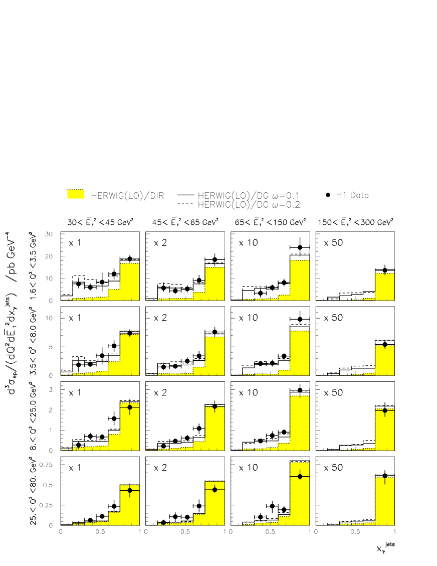
Figure 3: The differential dijet cross-section ${\rm d}^{3}\sigma_{ep}/{\rm d}Q^{2}{\rm d}\overline{E_{t}}^{2}{\rm d}x^{jets}_{\gamma}$ shown as a function of $x^{jets}_{\gamma}$ for different regions of $\overline{E_{t}}^{2}$ and $Q^{2}$. The scale factors applied to the cross-sections are indicated. The error bar shows the quadratic sum of systematic and statistical errors. The absence of a data point indicates that no measurement was made because of insufficient statistics for the two dimensional unfolding. Also shown is the HERWIG(LO)/DG model with 10% soft-underlying event and two choices of the $Q^{2}$ suppression factor $\omega$. The full histogram is for $\omega=0.1~{}{\rm GeV}$ and the dashed for $\omega=0.2~{}{\rm GeV}$. The direct component of this model is shown as the shaded histogram.

The corrected triple-differential cross-section for $0.1<y<0.7$ and for jets satisfying the criteria given in equations 10 – 13 is given in Tables  2 and 3 and is shown in Figures 3, 4 and 5 in various projections. The three Figures show the cross-section as functions of $x^{jets}_{\gamma}$, $\overline{E_{t}}^{2}$ and $Q^{2}$, respectively. In each case, the distributions are shown for ranges of the other two variables. The data are depicted as points with error bars. The error bars show the statistical and systematic errors added in quadrature. Note that the systematic errors are dominant everywhere. The absence of a data point indicates that no measurement was made in that bin because of insufficient statistics for the unfolding.

In Figure 3, the $x^{jets}_{\gamma}$ distributions can be seen to peak towards $x^{jets}_{\gamma}=1$, where the direct photon contribution is expected to be concentrated. There is a strong decrease in the cross-section with increasing $\overline{E_{t}}^{2}$. As $Q^{2}$ increases at fixed $\overline{E_{t}}^{2}$, the cross-section decreases and, for $\overline{E_{t}}^{2}<150\;{\rm GeV}^{2}$, the relative contribution from resolved photons, in the region $x^{jets}_{\gamma}\,\lower 1.07639pt\hbox{$\scriptstyle\sim$}\kern-5.59721pt\raise 2.36806pt\hbox{$\scriptstyle<$}\,0.75$, can be seen to diminish. For $\overline{E_{t}}^{2}>150\;{\rm GeV}^{2}$, only the highest $x^{jets}_{\gamma}$ point has been measured. Note that the reduction in the cross-section in the lowest $x^{jets}_{\gamma}$ bin is a consequence of the cuts in $\overline{\eta}$ and $\overline{E_{t}}^{2}$.

The data are compared with predictions of models with LO matrix elements and parton densities. The HERWIG(LO)/DG simulation is shown for two choices of the $Q^{2}$ suppression factor, $\omega$. The predictions for the direct only contribution are also shown. With $\omega=0.1\;{\rm GeV}$, the HERWIG(LO)/DG model gives a reasonable description of the cross-section throughout the $Q^{2}$-$\overline{E_{t}}^{2}$ range. Increasing $\omega$ to 0.2 GeV leads to an overestimation in the low $Q^{2}$, low $\overline{E_{t}}^{2}$ regions. The value of $\omega$ which best describes the data, however, depends on the frequency of soft underlying events. The RAPGAP(LO)/DG model prediction (not shown in this Figure), which contains no soft underlying event, requires $\omega$ $\sim 0.2\;{\rm GeV}$ in order to describe the data. As $Q^{2}$ increases, both HERWIG models tend to underestimate the cross-section for intermediate $x^{jets}_{\gamma}$ values and overestimate it at high $x^{jets}_{\gamma}$ The direct only contribution is able to describe the data in the highest $x^{jets}_{\gamma}$ bin but underestimates the data for $x^{jets}_{\gamma}\,\lower 1.07639pt\hbox{$\scriptstyle\sim$}\kern-5.59721pt\raise 2.36806pt\hbox{$\scriptstyle<$}\,0.75$ except possibly in the highest $Q^{2}$ range.

The $\overline{E_{t}}^{2}$ dependence of the cross-section is shown in Figure 4. It is compared with predictions from RAPGAP(LO) using three different choices for the photon parton densities. In the highest $x^{jets}_{\gamma}$ range, where direct processes are expected to dominate, all the models give a good description of the data. Elsewhere, the models provide a spread of predictions and no single one is preferred. The Drees-Godbole model tends to overestimate the cross-section for $1.6<Q^{2}<3.5\;{\rm GeV}^{2}$. For $Q^{2}>3.5\;{\rm GeV^{2}}$ and $0.45<x_{\gamma}<0.75$, all three models tend to underestimate the data but are still compatible within errors.

The $Q^{2}$ dependence of the cross-section is shown in Figure 5. There is a steep decrease in the cross-section with $Q^{2}$. The expectation from the direct photon component only of the RAPGAP(LO)/DG model shows a rate of suppression of the cross-section which is independent of $x^{jets}_{\gamma}$. However, the data show a rate of suppression which diminishes with increasing $x^{jets}_{\gamma}$. This behaviour is governed by the additional $Q^{2}$ suppression of the photon parton densities and the full RAPGAP(LO)/DG model including the resolved photon component gives a better description.

From the above comparisons we conclude that the observed dependence of the dijet cross-section is consistent with that predicted for a resolved virtual photon with parton density functions evolving with $Q^{2}$ according to QCD motivated models. In the next section we therefore proceed to extract an effective parton density for virtual photons from the data.

6 The effective parton density for virtual photons

6.1 Measurement of the Effective Parton Density

In order to measure the parton densities of the virtual photons we adapt the Single Effective Subprocess Approximation [31], originally developed for use in $p\overline{p}$ collisions and recently used to investigate real photon structure [3]. In LO, the cross-section for the production of dijets by resolved virtual photons can be written as:

$$\frac{{\rm d}^{5}\sigma}{{\rm d}y\;{\rm d}x_{\gamma}\;{\rm d}x_{\rm p}\;{\rm d}\cos\theta^{*}\;{\rm d}Q^{2}}=\qquad\qquad\qquad$$

$$\qquad\frac{1}{32\pi s_{\rm ep}}\,\,\sum_{k=T,L}\frac{f_{\gamma/{\rm e}}^{k}(y,Q^{2})}{y}\,\,\sum_{ij}\,\,\frac{f_{i/\gamma}^{k}(x_{\gamma},P_{t}^{2},Q^{2})}{x_{\gamma}}\,\,\frac{f_{j/{\rm p}}(x_{\rm p},P_{t}^{2})}{x_{\rm p}}\,\,|M_{ij}(\cos\theta^{*})|^{2}\;.$$ (15)

Here $f_{i/\gamma}^{T}$, $f_{i/\gamma}^{L}$ and $f_{i/{\rm p}}$ are the densities of parton species $i$ in transverse photons, longitudinal photons and the proton respectively. They are evaluated at the factorisation scale which we set equal to the renormalisation scale and choose to be $P_{t}^{2}$. The $M_{ij}$ are matrix elements for $2\rightarrow 2$ parton-parton hard scattering processes. The quantity $s_{{\rm ep}}$ is the square of the centre of mass energy in the ep collision, $\theta^{*}$ is the polar angle of the outgoing partons in the parton-parton centre of mass frame and $x_{\rm p}$ is the momentum fraction of the parton out of the proton. The fluxes of transverse and longitudinal photons are given by [32]:

$$f^{T}_{\gamma/e}(y,Q^{2}) = \frac{\alpha}{2\pi}\Bigl{[}\frac{1+(1-y)^{2}}{y}\frac{1}{Q^{2}}-\frac{2m_{e}^{2}y}{Q^{4}}\Bigr{]}$$

$$f^{L}_{\gamma/e}(y,Q^{2}) = \frac{\alpha}{2\pi}\frac{2(1-y)}{y}\frac{1}{Q^{2}}.$$ (16)

The measured dijet cross-sections do not allow us to separate the various parton sub-processes or photon polarisation states. To obtain a factorisable form, we first approximate equation (15) by:

$$\frac{{\rm d}^{5}\sigma}{{\rm d}y\;{\rm d}x_{\gamma}\;{\rm d}x_{\rm p}\;{\rm d}\cos\theta^{*}\;{\rm d}Q^{2}}\approx\qquad\qquad\qquad$$

$$\qquad\frac{1}{32\pi s_{\rm ep}}\,\,\frac{f_{\gamma/{\rm e}}^{T}(y,Q^{2})}{y}\,\,\sum_{ij}\,\,\frac{f_{i/\gamma}(x_{\gamma},P_{t}^{2},Q^{2})}{x_{\gamma}}\,\,\frac{f_{j/{\rm p}}(x_{\rm p},P_{t}^{2})}{x_{\rm p}}\,\,|M_{ij}(\cos\theta^{*})|^{2}\;,$$ (17)

We have defined a set of photon polarisation-averaged parton densities:

$$f_{i/\gamma}(x_{\gamma},P_{t}^{2},Q^{2}) \equiv f_{i/\gamma}^{T}(x_{\gamma},P_{t}^{2},Q^{2})+\overline{\epsilon}f_{i/\gamma}^{L}(x_{\gamma},P_{t}^{2},Q^{2}),$$ (18)

where $\overline{\epsilon}\sim 1$ is the ratio of longitudinal to transverse photon fluxes, averaged over the $y$-range of the data. $f_{i/\gamma}^{L}$ is expected to be small over most of the kinematic range considered here [7, 12, 33].

The Single Effective Subprocess (SES) approximation exploits the fact that the dominant contributions to the cross-section, namely $qg\rightarrow qg$, $gg\rightarrow gg$ and $qq\rightarrow qq$ t-channel processes, come from parton-parton scattering matrix elements that have similar shapes and so differ mainly by their associated colour factors. Thus the sum over processes can be replaced by a single effective sub-process cross-section and effective parton densities for the photon and proton:

$$\frac{{\rm d}^{5}\sigma}{{\rm d}y\;{\rm d}x_{\gamma}\;{\rm d}x_{\rm p}\;{\rm d}\cos\theta^{*}\;{\rm d}Q^{2}}\approx\qquad\qquad\qquad$$

$$\qquad\frac{1}{32\pi s_{\rm ep}}\,\,\frac{f_{\gamma/{\rm e}}^{T}(y,Q^{2})}{y}\,\,\frac{\tilde{f}_{\gamma}(x_{\gamma},P_{t}^{2},Q^{2})}{x_{\gamma}}\,\,\frac{\tilde{f}_{{\rm p}}(x_{\rm p},P_{t}^{2})}{x_{\rm p}}\,\,|M_{\rm SES}(\cos\theta^{*})|^{2}\;.$$ (19)

where the effective parton densities are

$$\tilde{f}_{\gamma}(x_{\gamma},P_{t}^{2},Q^{2}) \equiv \sum_{\rm n_{f}}\left(f_{{\rm q}/\gamma}(x_{\gamma},P_{t}^{2},Q^{2})+f_{\overline{\rm q}/\gamma}(x_{\gamma},P_{t}^{2},Q^{2})\right)+\frac{9}{4}\,f_{{\rm g}/\gamma}(x_{\gamma},P_{t}^{2},Q^{2})\;\;\;\;$$ (20)

$${\rm and}\quad\tilde{f}_{\rm p}(x_{\rm p},P_{t}^{2}) \equiv \sum_{\rm n_{f}}\left(f_{{\rm q}/{\rm p}}(x_{\rm p},P_{t}^{2})+f_{\overline{\rm q}/{\rm p}}(x_{\rm p},P_{t}^{2})\right)+\frac{9}{4}\,f_{{\rm g}/{\rm p}}(x_{\rm p},P_{t}^{2})\;$$ (21)

and the sums are over the quark flavours.

To extract the effective parton densities, the Bayesian unfolding method was applied again to correct the dijet cross-section to the diparton cross-section. This second unfolding corrects for hadronisation effects, the influence of the soft underlying event, and initial and final state QCD radiation. It uses correlations between the $\{x_{\gamma}^{jets},\overline{E}_{T}^{2}\}$ of the jets and $\{x_{\gamma},P_{t}^{2}\}$ of the parton-parton hard scattering, obtained using the HERWIG(LO)-DG simulation. Here we use LO parton densities and the 1-loop formula for $\alpha_{S}$ for a consistent leading-order treatment. The resolution in $x_{\gamma}$ varies from $15\%$ at low $x_{\gamma}$ to $10\%$ at high $x_{\gamma}$ in resolved events, and is $7\%$ in direct processes. The $P_{t}^{2}$ resolution is $40\%$ at low $P_{t}$ improving to $24\%$ at high $P_{t}$. The effective parton density was then determined by comparing the diparton cross-section measured in the data with that predicted by the simulations with a known set of photon parton densities:

$$\tilde{f}^{DATA}_{\gamma}=\tilde{f}^{MC}_{\gamma}\times\frac{({\rm d}^{3}\sigma_{ep}/{\rm d}Q^{2}{\rm d}P_{t}^{2}{\rm d}x_{\gamma})^{DATA}}{({\rm d}^{3}\sigma_{ep}/{\rm d}Q^{2}{\rm d}P_{t}^{2}{\rm d}x_{\gamma})^{MC}}$$ (22)

using equation 20 to evaluate $\tilde{f}^{MC}_{\gamma}$.

Now we discuss the systematic errors on the effective parton density. Additional systematic errors associated with the second unfolding were added in quadrature to those associated with determination of the triple-differential cross-section measurement described in the previous section. The most significant new systematic effects arise from the model dependences. These were estimated by repeating the second unfolding with RAPGAP and HERWIG varying the input parton densities, the amount of soft underlying event and the hadronisation models as detailed below.

• Model Dependence. Additional model dependences arising from the use of different parton showering and hadronisation mechanisms and different input parton densities were estimated by unfolding the data using the RAPGAP(LO)/SAS-1D, RAPGAP(LO)/SAS-2D and RAPGAP(LO)/DG models and comparing the results with those obtained after unfolding with HERWIG(LO)/DG. We assign a further 25% systematic error on the basis of this test, of which 20% arises from the hadronisation uncertainties.

• Unfolding Instability. Unfolding instabilities were estimated by varying the number of iterations and lead to a 10% uncertainty.

• Soft Underlying Event. The transformation from jet-based observables to parton variables is more strongly influenced by the presence of the soft underlying event than was the case for the transformation between true and measured jets. As an independent measure of the amount of soft underlying event we examine the transverse energy flow in the region outside the jets. In Figure 6 we show the transverse energy flow per unit area in the $(\eta,\phi)$ plane outside of circles of radius 1.3 about the two highest $E_{t}$ jets and in the range $-1.0<\eta<1.0$ as a function of $Q^{2}$. This central region of pseudo-rapidity is where transverse energy flow from remnant-remnant interactions is expected to be largest. The energy flow is corrected for detector effects. The inner error bars show the statistical errors and the outer error bars the quadratic sum of statistical and systematic errors. The latter include all the sources considered for the jet cross-section measurement. The observed decrease with increasing $Q^{2}$ is compared with predictions from HERWIG(LO)/DG with 0%, 5% and 10% soft underlying event and with RAPGAP(LO)/SAS-2D. Note that with the different choice of minimum $P_{t}$ and space-like shower parameter QSPAC (see section 3), which is used in HERWIG(LO)-DG for this step in the analysis, a lower soft underlying event frequency is required to describe the data.

  We varied the soft-underlying event probability in HERWIG between 0% and 10% in order to estimate the systematic uncertainty on the effective parton density. The resulting systematic error has a mean value of 20% and the error is largest at low $x_{\gamma}$ and low $Q^{2}$.

6.2 Discussion of the Extracted Effective Parton Density

The extracted effective parton density is given in Table 4 and shown in Figures 7, 8, and 9. The measurement uncertainties are everywhere domininated by the systematic errors. Only points where $\langle P_{t}^{2}\rangle>\langle Q^{2}\rangle$ are shown. It should be noted that in the highest $Q^{2}$ bins, $Q^{2}$ approaches $P_{t}^{2}$ and the assumptions of factorisation involved in the definition of a universal effective parton density begin to break down [7, 28]. Furthermore, the effects arising from higher twist contributions and longitudinally polarised photons are largest here. Nevertheless, we extract the effective parton distributions in the full region of the available data. The universality of the PDF’s extracted in the region where $Q^{2}$ is of the same order as $P_{t}^{2}$ will need to be demonstrated in other virtual photon induced reactions. The Figures show the evolution of the effective parton density in the photon both with the scale at which it is probed and with its virtuality. The data are compared with three sets of parton densities, SAS-1D, SAS-2D and the effective parton density calculated from the Drees-Godbole model using GRV-LO densities for the real photon and setting the free parameter, $\omega$, in the suppression factor to 0.1 GeV. The predictions were evaluated at the mean $x_{\gamma}$ and logarithmic mean $Q^{2}$ and $P_{t}^{2}$ of the ranges.

Figure 7 shows that the effective parton density tends to rise with $x_{\gamma}$ in the region studied. This shape is characteristic of photon structure. The data are described by all three models within errors except possibly in the two higher $Q^{2}$ ranges where the models tend to underestimate the data in the intermediate and high $x_{\gamma}$ bins.

In Figure 8, the parton density is shown as a function of the square of the probing scale $P_{t}^{2}$ in ranges of $x_{\gamma}$ and $Q^{2}$. The effective parton density is roughly independent of $P_{t}^{2}$ in each of the ranges. This scale dependence contrasts with the falling behaviour expected for hadronic parton densities and, within the rather large systematic errors, is consistent with the normalisation and logarithmic scale dependence predicted by perturbative QCD for the anomalous component of the photon.

The decrease of the parton density with virtuality is most clearly seen in Fig 9, where the $Q^{2}$ dependence is shown in ranges of $P_{t}^{2}$ and $x_{\gamma}$. The three parameterisations for the parton density all give a good description of the data both in the lowest $x_{\gamma}$ range and in the lowest two $Q^{2}$ bins. They all predict a more rapid suppression as $Q^{2}$ increases than is seen in the data. It is in this region where $Q^{2}\rightarrow P_{t}^{2}$ that non-leading terms, not accounted for in the models, are expected to become important and may affect the extraction of the effective parton distribution from these data.

In Figure 10, the $Q^{2}$ evolution of the effective parton density is shown for $P_{t}^{2}=85\;{\rm GeV}^{2}$, in the upper Figure for $0.35<x_{\gamma}<0.5$ and in the lower for $0.5<x_{\gamma}<0.7$. Superimposed on the same plots are photoproduction data at $P_{t}^{2}=112\;{\rm GeV}^{2}$ and $x_{\gamma}$ values of 0.3 and 0.55, taken from reference [3], which we have extrapolated to the $P_{t}^{2}$ and $x_{\gamma}$ values in the Figures. The extrapolation was based on the GRV-LO parton densities which give a good description of the photoproduction data. The evolution is compared with that predicted by the three models described above and also with a simple $\rho$-pole suppression factor characteristic of a pure VMD model:

$$f_{i|\gamma}(x_{\gamma},P_{t}^{2},Q^{2})\sim f_{i|\gamma}(x_{\gamma},P_{t}^{2},0)\Bigl{(}\frac{m_{\rho}^{2}}{m_{\rho}^{2}+Q^{2}}\Bigr{)}^{2}.$$ (23)

The latter clearly underestimates the data. The logarithmic suppression predicted by the virtual photon models on the other hand gives a good description below $Q^{2}\sim 20\;{\rm GeV}^{2}$. At higher $Q^{2}$ they predict a more rapid decrease than is seen in the data.

7 Conclusions

We have measured the triple-differential cross-section, ${\rm d}^{3}\sigma_{ep}/{\rm d}Q^{2}{\rm d}\overline{E_{t}}^{2}{\rm d}x^{jets}_{\gamma}$, in dijet events for $1.6<Q^{2}<80\;\rm{GeV}^{2}$ and $0.1<y<0.7$. The measured cross-sections show the $x^{jets}_{\gamma}$, $\overline{E_{t}}^{2}$ and $Q^{2}$ behaviour expected for processes in which a virtual photon, carrying a partonic structure evolving according to perturbative QCD, interacts with the proton via hard parton-parton scattering. The measurements are consistent with the perturbative QCD prediction that, as $Q^{2}\rightarrow\overline{E_{t}}^{2}$, the photon structure reduces to a simple direct coupling to $q\overline{q}$ pairs and the dijet cross-section is well-described without invoking photon structure. LO Monte Carlo models based on these QCD predictions give a good description of the data.

An effective, leading order, parton density of the virtual photon has been extracted in the Single Effective Subprocess approximation and its dependences on $x_{\gamma}$, probing scale $P_{t}^{2}$ and target virtuality $Q^{2}$ have been measured. The photon parton density is approximately independent of $p_{T}^{2}$ and, within errors, it is consistent with the normalisation and logarithmic scaling violations characteristic of photon structure. It is seen to be suppressed with increasing $Q^{2}$ as predicted by perturbative QCD.

$Q^{2}$ (${\rm GeV}^{2})$	$\overline{E_{t}}^{2}$ (${\rm GeV}^{2}$)	$x_{\gamma}$	$\sigma$ (pb)	Stat($\pm$)	Sys(+)	Sys(-)
1.6$<Q^{2}<$3.5	30$<\overline{E_{t}}^{2}<$45	0.15$<x_{\gamma}<$0.3	7.50	0.18	2.84	1.96
		0.3$<x_{\gamma}<$0.45	5.98	0.15	1.64	1.37
		0.45$<x_{\gamma}<$0.6	8.34	0.21	4.20	4.15
		0.6$<x_{\gamma}<$0.75	12.00	0.25	2.59	2.58
		0.75$<x_{\gamma}<$1.0	18.76	0.30	1.70	1.71
1.6$<Q^{2}<$3.5	45$<\overline{E_{t}}^{2}<$65	0.15$<x_{\gamma}<$0.3	2.81	0.11	1.28	0.78
		0.3$<x_{\gamma}<$0.45	2.20	0.09	0.85	0.70
		0.45$<x_{\gamma}<$0.6	2.62	0.08	0.78	0.75
		0.6$<x_{\gamma}<$0.75	4.58	0.11	1.21	0.97
		0.75$<x_{\gamma}<$1.0	9.22	0.19	1.38	1.51
1.6$<Q^{2}<$3.5	65$<\overline{E_{t}}^{2}<$150	0.3$<x_{\gamma}<$0.45	0.33	0.02	0.22	0.19
		0.45$<x_{\gamma}<$0.6	0.58	0.03	0.14	0.15
		0.6$<x_{\gamma}<$0.75	0.81	0.03	0.18	0.16
		0.75$<x_{\gamma}<$1.0	2.40	0.05	0.46	0.41
1.6$<Q^{2}<$3.5	150$<\overline{E_{t}}^{2}<$300	0.75$<x_{\gamma}<$1.0	0.27	0.01	0.05	0.04
3.5$<Q^{2}<$8.0	30$<\overline{E_{t}}^{2}<$45	0.15$<x_{\gamma}<$0.3	1.88	0.05	1.33	1.33
		0.3$<x_{\gamma}<$0.45	1.95	0.05	0.47	0.30
		0.45$<x_{\gamma}<$0.6	3.46	0.07	1.42	1.45
		0.6$<x_{\gamma}<$0.75	5.18	0.09	1.06	1.07
		0.75$<x_{\gamma}<$1.0	7.38	0.12	0.68	0.64
3.5$<Q^{2}<$8.0	45$<\overline{E_{t}}^{2}<$65	0.15$<x_{\gamma}<$0.3	0.75	0.03	0.36	0.29
		0.3$<x_{\gamma}<$0.45	0.81	0.02	0.22	0.18
		0.45$<x_{\gamma}<$0.6	1.27	0.04	0.31	0.29
		0.6$<x_{\gamma}<$0.75	1.72	0.05	0.43	0.46
		0.75$<x_{\gamma}<$1.0	3.80	0.07	0.46	0.43
3.5$<Q^{2}<$8.0	65$<\overline{E_{t}}^{2}<$150	0.3$<x_{\gamma}<$0.45	0.21	0.01	0.05	0.04
		0.45$<x_{\gamma}<$0.6	0.21	0.01	0.06	0.06
		0.6$<x_{\gamma}<$0.75	0.34	0.01	0.05	0.06
		0.75$<x_{\gamma}<$1.0	0.98	0.02	0.14	0.10
3.5$<Q^{2}<$8.0	150$<\overline{E_{t}}^{2}<$300	0.75$<x_{\gamma}<$1.0	0.11	0.01	0.02	0.02

Table 2: The triple-differential dijet cross-section ${\rm d}^{3}\sigma_{ep}/{\rm d}Q^{2}{\rm d}\overline{E_{t}}^{2}{\rm d}x^{jets}_{\gamma}$ for $0.1<y<0.7$ in ranges of $Q^{2}$, $\overline{E_{t}}^{2}$ and $x^{jets}_{\gamma}$. The cross-section in pb is given together with the statistical, positive systematic and negative systematic errors. The table shows measurements for $Q^{2}\leq 8.0~{}{\rm GeV}^{2}$. The higher $Q^{2}$ region is given in table 3.

$Q^{2}$ (${\rm GeV}^{2}$)	$\overline{E_{t}}^{2}$ (${\rm GeV}^{2}$)	$x_{\gamma}$	$\sigma$ (pb)	Stat($\pm$)	Sys(+)	Sys(-)
8.0$<Q^{2}<$25	30$<\overline{E_{t}}^{2}<$45	0.15$<x_{\gamma}<$0.3	0.27	0.01	0.21	0.20
		0.3$<x_{\gamma}<$0.45	0.670	0.02	0.17	0.18
		0.45$<x_{\gamma}<$0.6	0.670	0.01	0.16	0.14
		0.6$<x_{\gamma}<$0.75	1.58	0.03	0.35	0.34
		0.75$<x_{\gamma}<$1.0	2.13	0.03	0.41	0.38
8.0$<Q^{2}<$25	45$<\overline{E_{t}}^{2}<$65	0.15$<x_{\gamma}<$0.3	0.11	0.01	0.05	0.04
		0.3$<x_{\gamma}<$0.45	0.23	0.01	0.04	0.04
		0.45$<x_{\gamma}<$0.6	0.31	0.01	0.08	0.08
		0.6$<x_{\gamma}<$0.75	0.54	0.01	0.12	0.13
		0.75$<x_{\gamma}<$1.0	1.09	0.02	0.15	0.15
8.0$<Q^{2}<$25	65$<\overline{E_{t}}^{2}<$150	0.3$<x_{\gamma}<$0.45	0.047	0.002	0.01	0.011
		0.45$<x_{\gamma}<$0.6	0.074	0.003	0.022	0.020
		0.6$<x_{\gamma}<$0.75	0.091	0.003	0.014	0.012
		0.75$<x_{\gamma}<$1.0	0.298	0.005	0.031	0.038
8.0$<Q^{2}<$25	150$<\overline{E_{t}}^{2}<$300	0.75$<x_{\gamma}<$1.0	0.039	0.001	0.008	0.006
25$<Q^{2}<$80	30$<\overline{E_{t}}^{2}<$45	0.15$<x_{\gamma}<$0.3	0.021	0.001	0.033	0.033
		0.3$<x_{\gamma}<$0.45	0.065	0.005	0.019	0.017
		0.45$<x_{\gamma}<$0.6	0.114	0.006	0.025	0.026
		0.6$<x_{\gamma}<$0.75	0.236	0.007	0.081	0.078
		0.75$<x_{\gamma}<$1.0	0.433	0.007	0.087	0.086
25$<Q^{2}<$80	45$<\overline{E_{t}}^{2}<$65	0.15$<x_{\gamma}<$0.3	0.018	0.001	0.018	0.018
		0.3$<x_{\gamma}<$0.45	0.055	0.005	0.026	0.036
		0.45$<x_{\gamma}<$0.6	0.051	0.003	0.015	0.017
		0.6$<x_{\gamma}<$0.75	0.120	0.005	0.040	0.040
		0.75$<x_{\gamma}<$1.0	0.220	0.004	0.031	0.020
25$<Q^{2}<$80	65$<\overline{E_{t}}^{2}<$150	0.3$<x_{\gamma}<$0.45	0.010	0.001	0.005	0.005
		0.45$<x_{\gamma}<$0.6	0.024	0.001	0.006	0.009
		0.6$<x_{\gamma}<$0.75	0.020	0.001	0.005	0.005
		0.75$<x_{\gamma}<$1.0	0.060	0.001	0.008	0.004
25$<Q^{2}<$80	150$<\overline{E_{t}}^{2}<$300	0.75$<x_{\gamma}<$1.0	0.012	0.001	0.001	0.002

Table 3: The triple-differential dijet cross-section ${\rm d}^{3}\sigma_{ep}/{\rm d}Q^{2}{\rm d}\overline{E_{t}}^{2}{\rm d}x^{jets}_{\gamma}$ in ranges of $Q^{2}$, $\overline{E_{t}}^{2}$ and $x^{jets}_{\gamma}$. The cross-section in pb is given together with the statistical, positive systematic and negative systematic errors. The table shows measurements for $Q^{2}>8.0~{}{\rm GeV}^{2}$. The lower $Q^{2}$ region is given in table 2.

$Q^{2}$ (${\rm GeV}^{2}$)	$P_{t}^{2}$ (${\rm GeV}^{2}$)	$x_{\gamma}$	$\alpha^{-1}\tilde{f}_{\gamma}$	Stat($\pm$)	Sys(+)	Sys(-)
2.4	40.0	0.275	0.55	0.02	0.23	0.19
		0.425	0.60	0.02	0.15	0.12
		0.6	0.95	0.03	0.17	0.29
	52.0	0.275	0.59	0.02	0.32	0.19
		0.425	0.57	0.02	0.20	0.15
		0.6	0.93	0.03	0.19	0.18
	85.0	0.425	0.53	0.02	0.29	0.18
		0.6	0.98	0.03	0.21	0.26
5.3	40.0	0.275	0.33	0.01	0.15	0.15
		0.425	0.49	0.02	0.14	0.13
		0.6	0.82	0.03	0.13	0.30
	52.0	0.275	0.36	0.01	0.20	0.16
		0.425	0.50	0.02	0.14	0.15
		0.6	0.85	0.03	0.14	0.25
	85.0	0.425	0.64	0.02	0.19	0.21
		0.6	0.87	0.03	0.15	0.23
12.7	40.0	0.275	0.16	0.01	0.07	0.08
		0.425	0.42	0.02	0.09	0.19
		0.6	0.54	0.02	0.10	0.25
	52.0	0.275	0.18	0.01	0.09	0.09
		0.425	0.45	0.02	0.09	0.20
		0.6	0.62	0.03	0.10	0.23
	85.0	0.425	0.46	0.02	0.12	0.21
		0.6	0.74	0.03	0.14	0.27
40.0	85.0	0.425	0.43	0.04	0.09	0.27
		0.6	0.65	0.04	0.19	0.41

Table 4: The leading order effective parton density of the photon $x_{\gamma}\tilde{f}_{\gamma}=\sum_{\rm n_{f}}\left(f_{{\rm q}/\gamma}+f_{\overline{\rm q}/\gamma}\right)+\frac{9}{4}\,f_{{\rm g}/\gamma}$ , divided by the fine structure constant $\alpha$, for different values of $Q^{2}$, $P_{t}^{2}$ and $x_{\gamma}$. Statistical, positive systematic and negative systematic errors are given.

Figure 1: Examples of leading order Feynman diagrams of dijet production in $\gamma^{*}p$ collisions. In direct processes (left) all of the photon’s 4-momentum enters the hard collision. If the transverse momentum of the outgoing dijets (labelled jet 1 and jet 2 in the figures) is large compared with $Q^{2}$, the virtual photon may be resolved (right) with only a fraction $x_{\gamma}<1$ of the photon’s 4-momentum involved. The diagrams are applicable to dijet production with either real or virtual photons.

Figure 2: The observed transverse energy flow in $\phi$ with respect to the axes (located at $\phi=0$) of each of the two highest $E_{t}$ jets in the selected event sample for a slice $\mid\eta-\eta^{jet}\mid<1$. The result is shown for various ranges of $\eta$ and $E_{t}$ of the jets. The second jet is always chosen to have $\phi<0$, leaving the pedestal level clearly visible to the right of the jet core, in the region $\phi>0$. The data are compared with predictions from the HERWIG(HO)/DG simulation with 10% soft underlying event (dashed histogram) and with the RAPGAP(HO)/SAS-2D model.

Figure 4: The differential dijet cross-section ${\rm d}^{3}\sigma_{ep}/{\rm d}Q^{2}{\rm d}\overline{E_{t}}^{2}{\rm d}x^{jets}_{\gamma}$ shown as a function of $\overline{E_{t}}^{2}$ for different regions of $x^{jets}_{\gamma}$ and $Q^{2}$. The error bars show the quadratic sum of systematic and statistical errors. Also shown is the RAPGAP(LO) model with three choices of photon parton density. The DG model with GRV-LO real photon densities and $\omega=0.2~{}{\rm GeV}$ is shown as the full curve. The predictions with SAS-1D and SAS-2D are shown as the dashed and dot-dashed curves respectively.

Figure 5: The differential dijet cross-section ${\rm d}^{3}\sigma_{ep}/{\rm d}Q^{2}{\rm d}\overline{E_{t}}^{2}{\rm d}x^{jets}_{\gamma}$ shown as a function of $Q^{2}$ for different regions of $x^{jets}_{\gamma}$ and $\overline{E_{t}}^{2}$. The error bars show the quadratic sum of systematic and statistical errors. The prediction from the RAPGAP(LO)/DG model is shown as the full curve. The dashed curve shows the prediction for the direct photon processes in this model.

Figure 6: The average transverse energy per unit area in $\eta-\phi$ space in the range $-1.0<\eta<1.0$ and $0<\phi<2\pi$ in the $\gamma^{*}p$ cms as a function of $Q^{2}$ and outside the two highest $E_{t}$ jets. The data are corrected for detector effects. The inner error bars show the statistical errors and the outer error bars are the quadratic sum of the statistical and systematic errors. Also shown is the prediction from the HERWIG(LO)/DG model with three choices for the percentage of resolved events with a soft underlying event: 0% (dash-dotted), 5% (full) and 10% (dashed). The prediction from the RAPGAP(LO)/SAS-2D model is shown as the dotted curve.

Figure 7: The leading order effective parton density of the photon $x_{\gamma}\tilde{f}_{\gamma}=\sum_{\rm n_{f}}\left(f_{{\rm q}/\gamma}+f_{\overline{\rm q}/\gamma}\right)+\frac{9}{4}\,f_{{\rm g}/\gamma}$ , divided by the fine structure constant $\alpha$, as a function of $x_{\gamma}$ for different values of $Q^{2}$ and $P_{t}^{2}$. The data are displayed as points, with the inner error bar depicting the statistical error, and the total error bar the quadratic sum of statistical and systematic errors. In most bins the inner errors are contained within the data point marker. Also shown are the predictions from the DG model using GRV-LO real photon parton densities and $\omega=0.1~{}{\rm GeV}$ (solid line) and the SAS-1D (dashed line) and SAS-2D (dot-dashed line) parameterisations.

Figure 8: The leading order effective parton density of the photon $x_{\gamma}\tilde{f}_{\gamma}=\sum_{\rm n_{f}}\left(f_{{\rm q}/\gamma}+f_{\overline{\rm q}/\gamma}\right)+\frac{9}{4}\,f_{{\rm g}/\gamma}$ , divided by the fine structure constant $\alpha$, as a function of the squared parton transverse momentum, $P_{t}^{2}$, for different values of $Q^{2}$ and $x_{\gamma}$. The data are displayed as points, with the inner error bar depicting the statistical error, and the total error bar the quadratic sum of statistical and systematic errors. In most bins the inner errors are contained within the data point marker. Also shown are the predictions from the DG model using GRV-LO real photon parton densities and $\omega=0.1~{}{\rm GeV}$ (solid line) and the SAS-1D (dashed line) and SAS-2D (dot-dashed line) parameterisations.

Figure 9: The leading order effective parton density of the photon $x_{\gamma}\tilde{f}_{\gamma}=\sum_{\rm n_{f}}\left(f_{{\rm q}/\gamma}+f_{\overline{\rm q}/\gamma}\right)+\frac{9}{4}\,f_{{\rm g}/\gamma}$ , divided by the fine structure constant $\alpha$, as a function of $Q^{2}$ for different values of $P_{t}^{2}$ and $x_{\gamma}$. The data are displayed as points, with the inner error bar depicting the statistical error, and the total error bar the quadratic sum of statistical and systematic errors. In most bins the inner errors are contained within the data point marker. Also shown are the predictions from the DG model using GRV-LO real photon parton densities and $\omega=0.1~{}{\rm GeV}$ (solid line) and the SAS-1D (dashed line) and SAS-2D (dot-dashed line) parameterisations.

Figure 10: The leading order effective parton density of the photon $x_{\gamma}\tilde{f}_{\gamma}=\sum_{\rm n_{f}}\left(f_{{\rm q}/\gamma}+f_{\overline{\rm q}/\gamma}\right)+\frac{9}{4}\,f_{{\rm g}/\gamma}$ , divided by the fine structure constant $\alpha$, as a function of $Q^{2}$ for $P_{t}^{2}=85~{}{\rm GeV^{2}}$ and two values of $x_{\gamma}$. The data are displayed as points, with the inner error bar depicting the statistical error, and the total error bar the quadratic sum of statistical and systematic errors. The points at $Q^{2}=0$ are taken from reference [3] and extrapolated to the right $P_{t}^{2}$ and $x_{\gamma}$ values by scaling with factors derived from GRV-LO parton densities for real photons. Also shown are the prediction from the DG model using GRV-LO photon parton densities and $\omega=0.1~{}{\rm GeV}$ (solid line) and the SAS-1D (dashed line) and SAS-2D (dotted line) parameterisations. The dot-dashed curve shows the photoproduction data scaled by a $\rho$-pole factor (see text).

References

-
[1]
PLUTO Collab., Ch. Berger et al., Phys. Lett. B142 (1984) 111;
PLUTO Collab., Ch. Berger et al., Nucl. Phys. B281 (1987) 365;
PLUTO Collab., Ch. Berger et al., Phys. Lett. B107 (1981) 168;
JADE Collab., W. Bartel et al., Z. Phys. C24 (1984) 231;
TASSO Collab., M. Althoff et al., Z. Phys. C24 (1984) 231;
TPC/2 Collab., H. Aihara et al., Phys. Rev. Lett. 58 (1987) 97;
TPC/2 Collab., H. Aihara et al., Z. Phys. C34 (1987) 1;
AMY Collab., T. Sasaki et al., Phys. Lett. B252 (1990) 491;
OPAL Collab., R. Akers et al., Z. Phys. C61 (1994) 199;
AMY Collab., B. J. Kim et al., Phys. Lett. B325 (1994) 248;
TOPAZ Collab., H. Hayashii et al., Phys. Lett. B314 (1993) 149;
ALEPH Collab., D. Buskulic et al., Phys. Lett. B313 (1993) 509;
DELPHI Collab., P. Abreu et al., Phys. Lett. B342 (1995) 402. -
[2]
ZEUS Collab., M. Derrick et al.,
Phys. Lett. B322 (1994) 287;
H1 Collab., T. Ahmed et al., Nucl. Phys. B445 (1995) 195;
ZEUS Collab., M. Derrick et al., Phys. Lett. B384 (1996) 401;
ZEUS Collab., J. Breitweg et al., Eur. Phys. J. C1 (1998) 109. - [3] H1 Collaboration, C. Adloff et al., Eur. Phys. J. C1 (1998) 97.
- [4] H1 Collab., S. Aid et al., Z. Phys. C70 (1996) 17.
-
[5]
T. Uematsu and T. Walsh, Phys. Lett. B101 (1981) 263;
T. Uematsu and T. Walsh, Nucl. Phys. B199 (1982) 93;
G. Rossi, U. California at San Diego preprint UCSD-10P10-227 (1983);
G. Rossi, Phys. Rev. D29 (1984) 852. - [6] PLUTO Collab., Ch. Berger et al., Phys. Lett. B142 (1984) 119.
- [7] M. Glück, E. Reya and M. Stratmann, Phys. Rev. D54 (1996) 5515.
- [8] M. Klasen, G. Kramer and B. Pötter, Eur. Phys. J. C1 (1998) 261.
- [9] D. de Florian, C. Garcia Canal and R. Sassot, Z. Phys. C75 (1997) 265.
- [10] J. Chýla, J. Cvach, Proceedings of the Workshop 1995/96 on “Future Physics at HERA”, eds. G. Ingelman, A. de Roeck and R. Klanner, DESY 1996, Vol. 1, 545.
- [11] M. Drees and R. Godbole, Phys. Rev. D50 (1994) 3124.
- [12] F. Borzumati and G. Schuler, Z. Phys. C58 (1993) 139.
- [13] H1 Collaboration, C. Adloff et al., Phys. Lett. B415 (1997) 418.
-
[14]
For detailed studies, refer to:
M.Taševský, PhD Thesis, Prague, in preparation. - [15] H1 Collaboration, Di-Jet Event Rates in Deep-Inelastic Scattering at HERA, DESY preprint 98-076, submitted to Eur. Phys. J. C.
-
[16]
S.D. Ellis, D.E. Soper, Phys. Rev. D48 (1993) 3160;
S. Catani, Yu.L. Dokshitzer, M.H. Seymour and B.R. Webber, Nucl. Phys. B406 (1993) 187. - [17] H1 Collaboration, I. Abt et al., Nucl. Instr. and Meth. A386 (1997) 310 and 348.
- [18] H1 SPACAL Group, R. D. Appuhn et al., Nucl. Instr. and Meth. A386 (1997) 397.
- [19] H1 Calorimeter Group, B. Andrieu et al., Nucl. Instr. and Meth. A336 (1993) 460.
-
[20]
H1 Calorimeter Group, B. Andrieu et al., Nucl. Instr. and Meth.
A350 (1994) 57;
H1 Calorimeter Group, B. Andrieu et al., Nucl. Instr. and Meth. A336 (1993) 499. - [21] G. Marchesini et al., Comp. Phys. Comm. 67 (1992) 465.
-
[22]
H. Jung, Comp. Phys. Comm. 86 (1995) 147;
RAPGAP 2.06 manual, to be published. -
[23]
G. Marchesini and B. Webber, Nucl. Phys. B238 (1984) 1;
G. Marchesini and B. Webber, Nucl. Phys. B310 (1988) 461. -
[24]
T. Sjöstrand, Comp. Phys. Comm. 82 (1994) 74;
T. Sjöstrand, CERN-TH-7112-93 (Dec. 1993, revised Aug. 1994) - [25] M. Glück, E. Reya and A. Vogt, Z. Phys. C67 (1995) 433.
- [26] ZEUS Collab., J. Breitweg et al., Eur. Phys. J. C1 (1998) 109.
- [27] M. Glück, E. Reya and A. Vogt, Phys. Rev. D45 (1992) 3986.
- [28] T. Sjöstrand and G. A. Schuler, Phys. Lett. B376 (1996) 193.
- [29] S. Frixione and G. Ridolfi, Nucl. Phys. B507 (1997) 315.
- [30] G. D’Agostini, Nucl. Instr. and Meth. A362 (1995) 487.
- [31] B. V. Combridge, C. J. Maxwell, Nucl. Phys. B239 (1984) 429.
- [32] See for example, V. M. Budnev et al., Phys. Rep. C15 (1974) 181.
- [33] S. Frixione, M. Mangano, P. Nason and G. Ridolfi, Phys. Lett. B319 (1993) 339.