DELPHI Collaboration DELPHI 98-174 PHYS 813 WU B 98-39 7 December, 1998

The Strong Coupling:
Measurements and Running

S. Hahn

Fachbereich Physik, Bergische Universität-GH Wuppertal
Gaußstraße 20, 42097 Wuppertal, Germany
e-mail: s.hahn@cern.ch

Measurements of $\alpha_{s}$ from event shapes in $\mbox{e}^{+}\mbox{e}^{-}$ annihilation are discussed including recent determinations using experimentally optimized scales, studies of theoretically motivated scale setting prescriptions, and recently observed problems with predictions in Next to Leading Logarithmic Approximation. Other recent precision measurements of $\alpha_{s}$ are briefly discussed. The relevance of power terms for the energy evolution of event shape means and distributions is demonstrated. Finally a summary on the current results on $\alpha_{s}(M_{Z}^{2})$ and its running is given.

Plenary talk presented at the Hadron Structure’98

Stara Lesna, September 7-13, 1998

1 Introduction

Most of our current knowledge about the strong coupling and its running comes from the analysis of the process $\mbox{e}^{+}\mbox{e}^{-}$ $\rightarrow hadrons$ which is the simplest possible initial state for strong interaction. The energy scale of the process is exactly known and hadronic interaction is limited to the final state. For many observables the hadronization corrections are proportional $1/Q$ and therefore LEP with an energy range up to about $200\>\mbox{Ge\kern-0.43057ptV}$ in the year 2000 is an ideal laboratory for studying QCD. Due to the huge cross section at the $\rm Z^{0}$ resonance every LEP experiment collected several million hadronic events, serving for a precise determination of $\alpha_{s}(M_{Z}^{2})$. With the high energy data from LEP 2, the running of $\alpha_{s}$ and the influence of non-perturbative power terms on the observed quantities can be studied in detail.

2 Consistent Measurements of $\alpha_{s}$ from the Analysis of $\bf Z^{0}$ Data using Oriented Event Shapes

Within the recent analysis [1] of $\rm Z^{0}$ data by the DELPHI collaboration, the distributions of 18 different shape observables are determined as a function of the polar angle $\vartheta_{T}$ of the thrust axis with respect to the $\mbox{e}^{+}\mbox{e}^{-}$ beam direction. Since the definition of the thrust axis has a forward-backward ambiguity, $\cos\vartheta\geq 0$ has been chosen, $\cos\vartheta$ is called the event orientation. The definition of the observables studied can be found in [1]. The theoretical predictions in $\cal O$($\alpha_{s}^{2}$) are calculated using EVENT2 [2], which applies the matrix elements of the Leiden Group [3]. Using this program, the double differential cross section for any IR- and collinear safe observable $Y$ in $\mbox{e}^{+}\mbox{e}^{-}$ annihilation in dependence on the event orientation can be calculated:

$$\frac{1}{\sigma_{tot}}\frac{d^{2}\sigma(Y,\cos\vartheta)}{dYd\cos\vartheta} = \bar{\alpha}_{s}(\mu^{2})\cdot A(Y,\cos\vartheta)$$

$$+ \bar{\alpha}_{s}^{2}(\mu^{2})\cdot\Big{[}B(Y,\cos\vartheta)+(2\pi\beta_{0}\ln(x_{\mu})-2)A(Y,\cos\vartheta)\Big{]}$$

where $\bar{\alpha}_{s}=\alpha_{s}/2\pi$ and $\rm\beta_{0}=(33-2n_{f})/12\pi$. $\sigma_{tot}$ is the one loop corrected cross section for the process $\mbox{e}^{+}\mbox{e}^{-}$ $\rm\to$ hadrons. $\rm A$ and $\rm B$ denote the $\cal O$($\alpha_{s}$) and $\cal O$($\alpha_{s}^{2}$) QCD coefficient functions, respectively.

The dependence on the renormalization scale $\mu$ enters logarithmically in $\cal O$($\alpha_{s}^{2}$). The scale factor $x_{\mu}$ is defined by $\mu^{2}=x_{\mu}Q^{2}$ where $Q=M_{Z}$ is the center of mass energy. In $\cal O$($\alpha_{s}^{2}$), the running of the strong coupling $\alpha_{s}$ at the renormalization scale $\mu$ is given by

$$\alpha_{s}(\mu)=\frac{1}{\beta_{0}\ln\frac{\mu^{2}}{\Lambda^{2}}}\left(1-\frac{\beta_{1}}{\beta_{0}^{2}}\frac{\ln\ln\frac{\mu^{2}}{\Lambda^{2}}}{\ln\frac{\mu^{2}}{\Lambda^{2}}}\right)$$ (2)

where $\Lambda\equiv\Lambda_{\overline{MS}}^{(5)}$ is the QCD scale parameter computed in the $\overline{MS}$ scheme for $n_{f}=5$ flavors and $\beta_{1}=(153-19n_{f})/24\pi^{2}$. The renormalization scale $\mu$ is a formally unphysical parameter and should not enter at all into an exact infinite order calculation. However, within the context of a truncated finite order perturbative expansion for any particular process under consideration, the definition of $\mu$ depends on the renormalization scheme employed, and its value is in principle completely arbitrary.

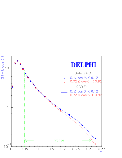
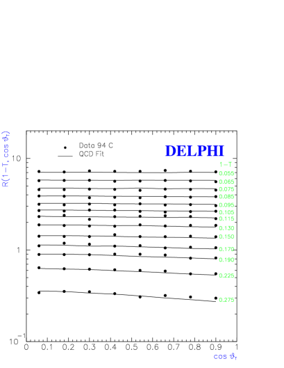
Figure 1: (a) QCD fits to the measured thrust distribution for two bins in $\rm\cos\vartheta_{T}$. (b) Measured thrust distribution at various fixed values of $\rm 1-T$ as a function of $\rm\cos\vartheta_{T}$. The solid lines represent the QCD fit.

The traditional experimental approach is, to measure all observables at the same, fixed scale value, the so-called physical scale (PHS) $\rm x_{\mu}=1$ or equivalently $\rm\mu^{2}=Q^{2}$. Applying PHS to the high precision DELPHI data at $\sqrt{s}=M_{Z}$ yields in general only a poor description of the measured event shape distributions, $\chi^{2}$ values up to $\chi^{2}/n_{df}\sim 40$ are found. For the PHS choice the $\rm 2^{nd}$ order contribution in Eq. 2 is in general quite large. For some observables the ratio of the $\cal O$($\alpha_{s}^{2}$) with respect to the $\cal O$($\alpha_{s}$) contribution $r_{NLO}$ is almost $\rm\left|r_{NLO}\right|\simeq 1.0$, indicating a poor convergence behavior of the corresponding perturbative expression. This quite naturally explains the observation of the wide spread of the measured $\alpha_{s}$ values for the individual observables (see Fig. 3b). If PHS is applied, an unweighted average for the $\alpha_{s}(M_{Z}^{2})$ values of the 18 observables yields $\chi^{2}/n_{df}=40/16$, i.e. the individual measurements are inconsistent. For the differential 2-jet rate determined using the Geneva-Algorithm, the fit applying $x_{\mu}=1$ fails completely to describe the data. Here, no $\alpha_{s}(M_{Z}^{2})$ value can be derived at all if PHS is applied. Therefore, the central method for measuring $\alpha_{s}(M_{Z}^{2})$ has been chosen to be a combined fit of $\alpha_{s}$ and the scale parameter $x_{\mu}$, a method known as experimentally optimized scales (EXP). Here one finds in general much smaller contributions from the $\cal O$($\alpha_{s}^{2}$) term in Eq. 2, indicating a better convergence behavior of the perturbative series. Applying EXP, the $\cal O$($\alpha_{s}^{2}$) predictions including the event orientation yield an excellent description of the high statistics data (see Fig. 1 as an example). For all observables considered, the QCD fit yields $\chi^{2}/n_{df}\simeq 1$.

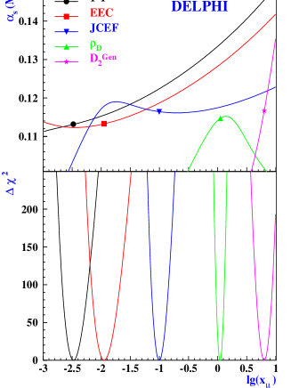
Figure 2: $\alpha_{s}(M_{Z}^{2})$ and $\Delta\chi^{2}=\chi^{2}-\chi^{2}_{min}$ from $\cal O$($\alpha_{s}^{2}$) fits for some of the observables studied as a function of the renormalization scale $x_{\mu}$. Additionally, the $\chi^{2}$ minima are indicated in the $\alpha_{s}(M_{Z}^{2})$ curves.

Fig. 2 shows the renormalization scale dependence of $\alpha_{s}(M_{Z}^{2})$ for some of the observables studied. It turns out that in order to describe the data, the scale has to be fixed to a rather narrow range of values. Consistent $\alpha_{s}(M_{Z}^{2})$ measurements can only be derived, if the optimized scale values $\bar{x}_{\mu}$ are applied, i.e. from the $\alpha_{s}$ values corresponding to the $\chi^{2}$ minima of the individual fits. For most of the observables the scale dependence in the vicinity of the $\chi^{2}$ minima is significantly reduced, but even for the few observables exhibiting a strong scale dependence around the $\chi^{2}$ minima, the corresponding $\alpha_{s}(M_{Z}^{2})$ values are perfectly consistent. The observable with the smallest scale dependence of $\alpha_{s}(M_{Z}^{2})$ is the Jet Cone Energy Fraction (JCEF) [4]. Here, the change in $\alpha_{s}(M_{Z}^{2})$ is only $\Delta\alpha_{s}(M_{Z}^{2})$ $=\pm 0.0010$, even if the scale is varied within the large range of $\bar{x}_{\mu}/2\leq x_{\mu}\leq 1.$ Additionally JCEF has the smallest hadronization correction uncertainties as well.

The $\alpha_{s}(M_{Z}^{2})$ values determined from 18 different observables are shown in Fig. 3 for EXP in comparison with PHS. For EXP the scatter among the different observables is significantly reduced. The errors of $\alpha_{s}(M_{Z}^{2})$ correspond to the quadratic sum of the uncertainty from the fit, the systematic experimental uncertainty and the hadronization uncertainty. Conservatively, an additional uncertainty due to the variation of the central renormalization scale value $\bar{x}_{\mu}$ between $0.5\cdot\bar{x}_{\mu}$ and $2.\cdot\bar{x}_{\mu}$ has been considered for both methods PHS and EXP. An unweighted average yields $\alpha_{s}(M_{Z}^{2})$ $=0.1165\pm 0.0026$ for EXP to be compared with $\alpha_{s}(M_{Z}^{2})$ $=0.1243\pm 0.0080$ in the case of PHS. The corresponding $\chi^{2}$ value is $\chi^{2}/n_{df}=7.3/17$ for EXP and $\chi^{2}/n_{df}=79/16$ for PHS. It should be emphasized, that the consistency for EXP does not depend on the additional uncertainty due to renormalization scale variation. Ignoring this uncertainty yields an consistent average value of $\alpha_{s}(M_{Z}^{2})$ as well ($\chi^{2}/n_{df}=9.2/17$). A weighted average of $\alpha_{s}(M_{Z}^{2})$ considering correlations between the observables yields $\alpha_{s}(M_{Z}^{2})$ $=0.1164\pm 0.0025$, almost identical to the unweighted average. The investigation of the influence of heavy quark mass effects on $\alpha_{s}(M_{Z}^{2})$ is under study. A preliminary estimate yields $\alpha_{s}(M_{Z}^{2})$ $=0.117\pm 0.003$.

     

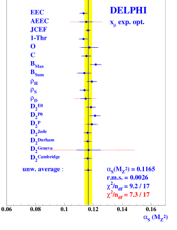
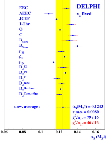
Figure 3: Results of the $\alpha_{s}(M_{Z}^{2})$ measurements from 18 event shape distributions. (a) fits using experimentally optimized scale values, (b) fixed scale fits : $x_{\mu}=1$. The errors on $\alpha_{s}(M_{Z}^{2})$ indicated correspond to the quadratic sum of the uncertainty from the fit, the systematic experimental uncertainty and the hadronization uncertainty. The dotted error bars indicate the additional uncertainty due to the variation of the central renormalization scale value $x_{\mu}$ between $0.5\cdot x_{\mu}$ and $2.\cdot x_{\mu}$.

2.1 Theoretically Motivated Scale Setting Methods

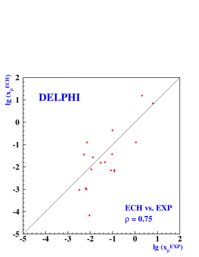
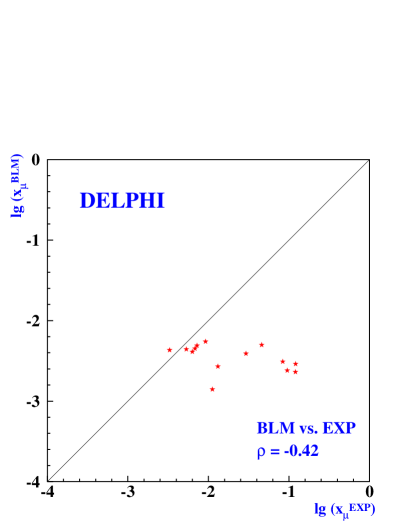
Figure 4: Correlation of experimentally optimized renormalization scale values with values predicted by theoretically motivated scale setting prescriptions. (left side: ECH method, right side: BLM approach)

Additional studies [1] have been made using theoretically motivated scale setting prescriptions, like the principle of minimal sensitivity (PMS), the method of effective charges (ECH) and the method of Brodsky, Lepage and MacKenzie (BLM). In the case of PMS and ECH, a strong correlation with the measured scale values from EXP can be observed. For the BLM method no such correlation is observed (see Fig. 4). Moreover, the BLM fits do not converge for some of the observables under study. The individual $\alpha_{s}$ values from the remaining observables turn out to be inconsistent. However, the average values of $\alpha_{s}(M_{Z}^{2})$ for all methods considered are consistent with EXP, but the scatter of the individual $\alpha_{s}(M_{Z}^{2})$ measurements is somewhat larger for the theoretically motivated methods.

The influence of higher order contributions has also been investigated [1] by using the method of Padé Approximants for the estimate of the uncalculated $\cal O$($\alpha_{s}^{3}$) contributions (PAP). In comparison with $\cal O$($\alpha_{s}^{2}$), the renormalization scale dependence for PAP is significantly reduced. Here, a fixed scale value of $x_{\mu}=1$ has been chosen for the $\alpha_{s}(M_{Z}^{2})$ measurements from the individual observables. The average value of $\alpha_{s}(M_{Z}^{2})$ is again in perfect agreement with the $\cal O$($\alpha_{s}^{2}$) result, suggesting small contributions due to missing higher order predictions.

2.2 Comparison with NLLA predictions

The probably most relevant check on the influence of higher order contributions comes from a study of the all orders resummed next to leading logarithmic approximation (NLLA), which has been calculated for a limited number of observables. Two different strategies have been applied [1]. Pure NLLA calculations have been used to measure $\alpha_{s}(M_{Z}^{2})$ in a limited kinematical region close to the infrared limit, where the logarithmic contributions become large. Matched NLLA + $\cal O$($\alpha_{s}^{2}$) calculations have been used to extend the $\cal O$($\alpha_{s}^{2}$) fit range towards the 2-jet region. Unlike $\cal O$($\alpha_{s}^{2}$) theory, no optimization is involved in adjusting the renormalization scale for NLLA predictions. Therefore the renormalization scale value has been fixed to $x_{\mu}=1$. Both methods yield average values of $\alpha_{s}(M_{Z}^{2})$ compatible with the average from $\cal O$($\alpha_{s}^{2}$), the scatter of the individual measurements is somewhat larger for the resummed theory.

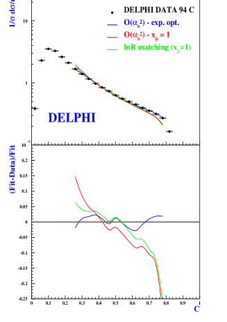
Figure 5: Comparison of the measured C-Parameter Distribution with three different QCD Fits: i) $\cal O$($\alpha_{s}^{2}$) using an experimentally optimized renormalization scale, ii) $\cal O$($\alpha_{s}^{2}$) using a fixed renormalization scale $\rm x_{\mu}=1$ and iii) $\ln R$ matched NLLA ($\rm x_{\mu}=1$) for the C Parameter. The lower part shows the relative difference (Fit-Data)/Fit. Whereas the $\cal O$($\alpha_{s}^{2}$) curve describes the data over the whole fit range, the slope of the curves for the fixed scale and $\ln R$ matching show a similar systematic distortion with respect to the data.

Looking at the individual measurements, one finds that the $\alpha_{s}$ values derived from matched predictions are systematically higher than those from pure NLLA theory. For some of the observables, the $\alpha_{s}$ value from matched predictions are even higher than for both pure NLLA and $\cal O$($\alpha_{s}^{2}$) predictions. Clearly the matched result is expected to be a kind of average of the results from both the distinct theories. Moreover, the matched theory predictions for some of the observables yield only a poor description of the high precision data, a more detailed investigation reveals a systematic deviation of the predicted slope with respect to the data (see Fig. 5). The distortion observed is similar to the distortion obtained using $\cal O$($\alpha_{s}^{2}$) predictions applying a fixed renormalization scale value of $x_{\mu}=1$, indicating that the terms included from the $2^{nd}$ order predictions dominate the matched predictions. Whereas $x_{\mu}=1$ seems to be an appropriate choice for pure NLLA predictions, the similarity of the two fit curves indicate a mismatch of the renormalization scale values for the $\cal O$($\alpha_{s}^{2}$) and NLLA part of the combined prediction.

3 Other High Precision $\alpha_{s}$ Measurements

3.1 $\alpha_{s}$ Determination from Precision Electroweak Measurements

The precise electroweak measurements performed at LEP and SLD can be used to check the validity of the Standard Model and to infer information about its fundamental parameters. Within the Standard Model fits of the LEP Electroweak Working Group, the value of $\alpha_{s}(M_{Z}^{2})$ depends mainly on $R_{l}$, $\Gamma_{Z}$ and $\sigma_{had}$. The theoretical prediction is known in NNLO-Precision. A recent update of the fit results presented at the ICHEP’98 [5] yields a value for the strong coupling of $\alpha_{s}(M_{Z}^{2})$ $=0.119\pm 0.003_{Fit}\pm 0.002_{Theo}$.

3.2 $\alpha_{s}$ Determination from Spectral Functions in Hadronic $\tau$ Decays

One of the few processes, where QCD predictions are known in NNLO, is the hadronic decay of the $\tau$ Lepton. Within the recent OPAL analysis [6], $\alpha_{s}$ has been determined from the moments of the spectral functions of the vector and axial-vector current in hadronic $\tau$ decays, which are weighted integrals over the differential decay rate $dR_{\tau,V/A}/ds$ for vector (V) and axial-vector (A) decays:

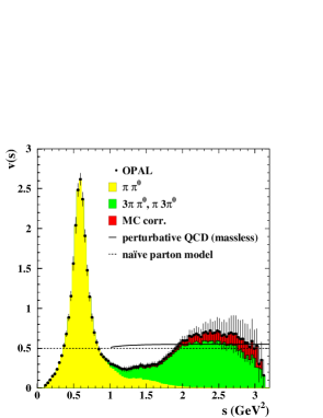
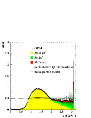
Figure 6: The vector and axial-vector spectral functions in hadronic $\tau$decays. The data points correspond to the sum of all contributing channels. Some exclusive contributions are shown as shaded areas.

$$R^{kl}_{\tau,V/A}(s_{0})=\int\limits_{0}^{s_{0}}ds\left(1-\frac{s}{s_{0}}\right)^{k}\left(\frac{s}{m_{\tau}^{2}}\right)^{l}dR_{\tau,V/A}/ds$$ (3)

The analysis involves a measurement of the invariant mass of the hadronic system and thus requires an exclusive reconstruction of all hadronic final states. After unfolding the measured spectra, normalizing them to their branching ratios and summing them up with their appropriate weights, one obtains the spectral functions shown in Fig. 6.

The QCD predictions have been calculated including perturbative and non-perturbative contributions. Within the framework of the Operator Product Expansion (OPE) the non-perturbative contributions are expressed as a power series in terms of $1/m_{\tau}^{2}$. In contrast to the perturbative part, the power corrections differ for the vector and axial-vector part, thus the difference of the vector and axial-vector spectral function is sensitive to non-perturbative effects only. The perturbative contribution is known in $\cal O$($\alpha_{s}^{3}$) and partly known in $\cal O$($\alpha_{s}^{4}$). On a first glance this accuracy looks quite impressive, it should however be emphasized, that with the small momentum transfers involved, the divergence of the perturbative series is a much more important issue for the $\tau$ decay than for $\alpha_{s}$ measurements at high energies. Recent estimates of the complete $\cal O$($\alpha_{s}^{4}$) contribution[8] to the perturbative prediction by the means of Padé Approximation predict an $\cal O$($\alpha_{s}^{4}$) contribution of about 20 % w.r.t. the leading order term, indicating that further higher-order terms could have a significant effect on the perturbative prediction. Three different calculations for the perturbative prediction have been studied within the OPAL analysis. Apart from the standard fixed order perturbative expansion (FOPT), two attempts have been studied to obtain a resummation of some of the higher order terms. The so-called contour improved perturbative theory (CIPT) accounts on higher order logarithmic terms in $\alpha_{s}$ by expressing the perturbative prediction by contour-integrals, which are evaluated numerically using the solution of the renormalization group equation (RGE) to four-loops. The third calculation includes an all order resummation of renormalon contributions in the so-called large $\beta_{0}$-limit (RCPT). This strategy has the advantage to be renormalization scheme invariant.

Prediction                       $\alpha_{s}(M_{Z}^{2})$                        $\chi^{2}/n_{df}$ (Fit 1) $\chi^{2}/n_{df}$ (Fit 2)
FOPT	$0.1191\pm 0.0008_{exp}\pm 0.0013_{theo}\pm 0.0003_{evol}$	$0.17/1$	$0.62/4$
CIPT	$0.1219\pm 0.0010_{exp}\pm 0.0017_{theo}\pm 0.0003_{evol}$	$0.16/1$	$0.63/4$
RCPT	$0.1169\pm 0.0007_{exp}\pm 0.0015_{theo}\pm 0.0003_{evol}$	$0.07/1$	$0.61/4$

Table 1: Results on $\alpha_{s}(M_{Z}^{2})$ from an OPAL analysis of spectral functions in hadronic $\tau$ decay. Given are the $\alpha_{s}(M_{Z}^{2})$ values for the three different perturbative calculations studied. The $\alpha_{s}(M_{Z}^{2})$ values for the two different fits are identical. Shown are also the $\chi^{2}/n_{df}$ values for both fit strategies.

Two different fits to the data have been performed. The first fit uses 5 moments from the sum of the vector and axial-vector spectral function for the determination of $\alpha_{s}(m_{\tau}^{2})$ together with three parameters from OPE, the second fit uses 10 moments and applies the vector and axial-vector functions separately for the determination of $\alpha_{s}(m_{\tau}^{2})$ in combination with 5 parameters from OPE. Both fits yield nearly identical results for $\alpha_{s}(m_{\tau}^{2})$. The $\alpha_{s}$ values are extrapolated to $M_{Z}$ using the RGE, the results for $\alpha_{s}(M_{Z}^{2})$ are summarized in table 1. The three different approaches describe the data equally well, the theoretical errors as well as the overall error is nearly the same, so from an experimental point of view there is no preferred calculation. However, the difference of the $\alpha_{s}$ values measured applying different theoretical assumptions is about 4 % i.e. the difference is much larger than the the theoretical error determined for each method. The reason for this is most likely due to underestimation of the uncertainty due to missing higher order terms. For the $\alpha_{s}(m_{\tau}^{2})$ determination, the renormalization scale value $x_{\mu}=\mu^{2}/m_{\tau}^{2}$ has been fixed to $\rm x_{\mu}=1$, an uncertainty has been estimated due to scale variation in the range $\rm 0.4\leq x_{\mu}\leq 2$, which is nearly the same range as in the DELPHI analysis of $\mbox{e}^{+}\mbox{e}^{-}$ event shapes. However, within the DELPHI analysis it turned out, that this scale variation range is sufficient only if one applies experimentally optimized scales, but yields inconsistent results for fixed scale values. An uncertainty due to the scheme dependence of the RGE coefficient $\beta_{3}$, which has been applied using the $\overline{MS}$ value, has been estimated due to variation between $0.\leq\beta_{3}^{RS}/\beta_{3}^{\overline{MS}}\leq 2.$, however there is no theoretical reason, why its value should not be negative. This is indeed sometimes the case if optimized renormalization schemes are applied (se e.g. [9]). A similar analysis done by the ALEPH collaboration[7] has shown, that the use of the PMS scheme optimization leads to an reduced value of $\alpha_{s}(M_{Z}^{2})$ and therefore reduces the discrepancy between FOPT and RCPT. Since the renormalization scheme optimization turns out to be of major importance in $\mbox{e}^{+}\mbox{e}^{-}$ annihilation, it would clearly be desirable to do similar studies in the analysis of hadronic $\tau$-decays.

3.3 $\alpha_{s}$ Determination from the Gross-Llewellyn-Smith Sum Rule in $\nu$-N-DIS

The Gross-Llewellyn-Smith (GLS) Sum Rule predicts the integral over the non-singlet structure function $xF_{3}(x,Q^{2})$ measured in $\nu$-N deep inelastic scattering. In the naive quark parton model, the value of this integral should be three. QCD corrections have been calculated in NNLO:

$$\int\limits_{0}^{1}xF_{3}(x,Q^{2})\frac{dx}{x}=3\left[1-\frac{\alpha_{s}}{\pi}-a(n_{f})(\frac{\alpha_{s}}{\pi})^{2}-b(n_{f})(\frac{\alpha_{s}}{\pi})^{3}\right]-\frac{\Delta HT}{Q^{2}}$$ (4)

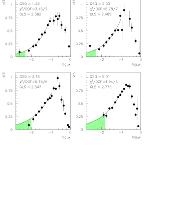
Figure 7: $xF_{3}$ as a function of $x$ at the four lowest $Q^{2}$ values. The curve shows a power law fit to the points with $x<0.1$, which is used to calculate the integral in the shaded regions.

The recent CCFR/NuTeV analysis [10] covers an energy range of $1\>\mbox{Ge\kern-0.43057ptV}^{2}<Q^{2}<15\>\mbox{Ge\kern-0.43057ptV}^{2}$ with $\langle Q^{2}\rangle\simeq 3\>\mbox{Ge\kern-0.43057ptV}^{2}$. The dominant error comes from the contribution of higher twist terms $\Delta HT$, which have been estimated to $\Delta HT=0.15\pm 0.15\>\mbox{Ge\kern-0.43057ptV}^{2}$. The GLS integral is evaluated using the $xF_{3}$ data separately in different $Q^{2}$ bins. For very low $x$ the data have been extrapolated using a power law fit (see fig. 7). Evolving the fit result for $\alpha_{s}(3\>\mbox{Ge\kern-0.43057ptV}^{2})$ to $M_{Z}^{2}$ yields $\alpha_{s}(M_{Z}^{2})$ = $0.114\pm^{.005}_{.006}(stat)\pm^{.007}_{.009}(syst)\pm.005(theo)$, which is consistent with other precise $\alpha_{s}$ determinations in different energy ranges.

3.4 $\alpha_{s}$ Determination in $\nu$-N-DIS from high $x$ scaling violations

Another $\alpha_{s}$ determination in $\nu$-N-DIS within an updated analysis of the CCFR collaboration [11] comes from a simultaneous fit of the $F_{2}$ and $xF_{3}$ structure functions. The QCD predictions are known in NLO. Improvements w.r.t. previous analyses are due to the new energy calibration and the higher energy and statistics of the experiment. The energy range of the data used for the $\alpha_{s}$ determination is $5\>\mbox{Ge\kern-0.43057ptV}^{2}<Q^{2}<125\>\mbox{Ge\kern-0.43057ptV}^{2}$. The fit yields $\alpha_{s}(M_{Z}^{2})$ = $0.119\pm 0.002(exp)\pm 0.001(HT)\pm 0.004(scale)$. The precision is better than from the NNLO analysis applying the GLS sum rule.

The result can e.g. be compared with a result of similar precision from the analysis of the $F_{2}$ structure function data from SLAC/BCDMS[12]. Within this analysis $\alpha_{s}$ has been determined to $\alpha_{s}(M_{Z}^{2})$ = $0.113\pm 0.003(exp)\pm 0.004(theo)$. Within both analyses, the renormalization scale value has been chosen to $x_{\mu}=1$. For an estimate of the scale uncertainty, $x_{\mu}$ has been varied within a large range of $0.1\leq x_{\mu}\leq 4.0$. A similar variation has been done also for the factorization scale uncertainty. The range for the scale variation has been chosen in such a way, that the $\chi^{2}$ of the fit is not significantly increased, indicating that the choice $x_{\mu}=1$ for the central result is appropriate for the analysis of structure functions in DIS.

4 Running of $\alpha_{s}$

The running of the strong coupling $\alpha_{s}$ is among the most fundamental predictions of QCD. Due to the large energy range covered by LEP1/2, this prediction can now be tested from $\mbox{e}^{+}\mbox{e}^{-}$ data, measured within a single experiment. Whereas the perturbative predictions lead to an approximately logarithmic energy dependence of event shapes, the hadronization process causes an inverse power law behavior in energy and can therefore be disentangled from the perturbative part by studying the energy evolution of event shapes. Traditionally, hadronization corrections are calculated by phenomenological Monte Carlo (MC) models, whose predictions can now precisely been tested over a large energy range. Although MC-models yield a good description of the measured data within a large energy range (see e.g. [14]), their predictive power suffers from a large number of free parameters, which have to be tuned to the data (e.g. 10-15 main parameters to be tuned within the JETSET partonshower model). A novel way in understanding the hadronization process has been achieved with the Dokshitzer-Webber (DW) model[13], which has recently been improved by results from 2-loop-calculations. Within this model, the power behaving contributions can be calculated, leaving only a single non-perturbative parameter to be determined from the data.

4.1 Power Corrections and the Dokshitzer-Webber model

Non-perturbative power corrections in the spirit of the DW-model arise from soft gluon radiation at energies of the order of the confinement scale. The leading power behavior is quantified by a non-perturbative parameter $\alpha_{0}$, defined by

$$\alpha_{0}(\mu_{I})=\frac{1}{\mu_{I}}\int\limits_{0}^{\mu_{I}}\alpha_{s}(k)dk$$ (5)

which is expected to be approximately universal. Here, the true coupling $\alpha_{s}(k)$ is assumed to be infrared regular and can be understood as the sum of two terms

$$\alpha_{s}(k)=\alpha_{s}^{PT}(k)+\alpha_{s}^{NP}(k)$$ (6)

where the perturbative part $\alpha_{s}^{PT}$ is separated from the non-perturbative part $\alpha_{s}^{NP}$ by an infrared matching scale $\mu_{I}$ of the order of a few  GeV. It is expected, that the factorial growing divergence of the fixed order perturbative expansion gets cancelled due to the merging with the non-perturbative counter-part, yielding a renormalon free theory.

For the shape observables $Y$ studied so far, the DW-model predicts the effect of the power corrections to be a simple shift of the perturbative distribution, i.e. for $Y=1-T,C,M_{H}$:

$$\frac{d\sigma}{dY}(Y)=\frac{d\sigma^{pert.}}{dY}(Y-c_{Y}{\cal P})$$ (7)

with an observable dependent factor $c_{Y}$ and $\cal P$ proportional $1/Q$:

$${\cal P}=\frac{4C_{F}}{\pi^{2}}{\cal M}\frac{\mu}{Q}\left[\alpha_{0}(\mu_{I})-\alpha_{s}(\mu)-\frac{\beta_{0}}{2\pi}\left(ln\frac{\mu}{\mu_{I}}+\frac{K}{\beta_{0}}+1\right)\right]$$ (8)

For the jet broadening observables $Y=B_{W},B_{T}$ the shift is predicted to be

$$\frac{d\sigma}{dY}(Y)=\frac{d\sigma^{pert.}}{dY}(Y-c_{Y}{\cal P}ln\frac{B}{B_{0}})$$ (9)

with an additional non-perturbative parameter $\alpha^{\prime}_{0}$ and a term ${\cal P}^{\prime}$ entering via the log-enhanced term. Within the re-analysis of the JADE-data[15] it turned out that in order to describe the transition from the perturbative predictions to the observed spectra of the jet broadening observables, not only a shift, but also a squeeze of the partonic distribution is required. The original calculations for the jet broadening observables are considered to be erroneous, however the problem seems to be solved now[16].

4.2 Power Corrections to mean event shapes

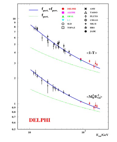
Figure 8: left side: Measured mean values of $1-T$ and $M_{H}$ from DELPHI high energy data and low energy data from various experiments. The solid lines represent the QCD fits in $\cal O$($\alpha_{s}^{2}$) applying the DW-model, the dotted lines show the perturbative contributions only. right side: $\langle 1-T\rangle$ distribution from an ALEPH analysis. The solid line represents a QCD fit in $\cal O$($\alpha_{s}^{2}$) applying the DW-model the dashed line represents a fit applying MC hadronization corrections.

Analysis	Observable	$\alpha_{0}(2\>\mbox{Ge\kern-0.43057ptV})$	$\alpha_{s}(M_{Z}^{2})$	$\chi^{2}/n_{df}$
DW-model (DELPHI)	$\langle 1-T\rangle$	$0.494\pm 0.009$	$0.1176\pm 0.0057$	43/22
DW-model (DELPHI)	$\langle M_{H}\rangle$	$0.558\pm 0.025$	$0.1172\pm 0.0037$	2/11
DW-model (ALEPH)	$\langle 1-T\rangle$	$0.497\pm 0.009^{*}$	$0.1184\pm 0.0019^{*}$	28/30
MC-corr.   (ALEPH)	$\langle 1-T\rangle$	$-$	$0.1307\pm 0.0005^{*}$	66/31

Table 2: Results of QCD fits in $\cal O$($\alpha_{s}^{2}$) to the mean values of event shapes at different $E_{cm}$. Hadronization corrections have been applied either by the means of the DW-model or as predicted by MC. ^∗Statistical errors only.

The earliest predictions from the DW-model have been made for the mean values of event shape distributions. In the context of the analysis of LEP2 data they have the advantage to make use of the full data statistics. Fig. 8 shows QCD fits in $\cal O$($\alpha_{s}^{2}$) applying the DW-model to mean event shapes measured at various $E_{cm}$, done by DELPHI[14] and ALEPH[17]. The fit results are listed in table 2. For the two observables studied, universality of $\alpha_{0}$ is found on a 10 % level. Apart from a somewhat poor fit quality for the $\langle 1-T\rangle$ data used by the DELPHI collab., which can be explained by the poor quality of the low energy data, the DW-model fits yield a good description of the data, which is even better than for MC hadronization corrections. The $\alpha_{s}(M_{Z}^{2})$ values obtained applying the DW model are in remarkable good agreement with $\alpha_{s}(M_{Z}^{2})$ as determined by the DELPHI analysis of $\mbox{e}^{+}\mbox{e}^{-}$ event shapes at the $\rm Z^{0}$. There is however a fundamental difference between both analyses: Whereas the analysis of $\rm Z^{0}$ data applies experimentally optimized scales in combination with MC hadronization corrections, the analysis applying the DW-model applies fixed scale values $x_{\mu}=1$, since a scale optimization is not feasible in this case. However, the fit quality of the DW-model fits indicate, that $x_{\mu}=1$ is an appropriate choice. The ALEPH result for the QCD fit to the $\langle 1-T\rangle$ distribution applying MC hadronization corrections is also listed in table 2. Here, again $x_{\mu}=1$ has been applied. The fit quality is quite poor and $\alpha_{s}(M_{Z}^{2})$ is much larger. The same observation has been made within the DELPHI $\rm Z^{0}$ analysis, and the result is just another demonstration, that fixed scale values are not qualified for an analysis applying MC corrections.

4.3 Power Corrections to event shape distributions

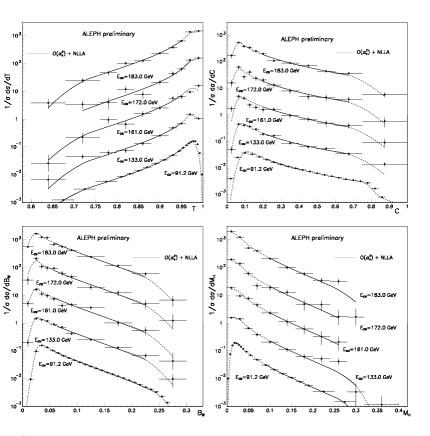
Figure 9: left side: Measured distributions of Thrust, C-Parameter, wide jet broadening and the heavy jet mass from ALEPH data between $91.2\>\mbox{Ge\kern-0.43057ptV}\leq E_{cm}\leq 183\>\mbox{Ge\kern-0.43057ptV}$. The lines represent a QCD fit applying the DW-model to shape distributions in matched $\cal O$($\alpha_{s}^{2}$) and NLLA precision. right side: QCD fits to the C-Parameter in matched $\cal O$($\alpha_{s}^{2}$) and NLLA precision applying DW power corrections to JADE and LEP data between $35\>\mbox{Ge\kern-0.43057ptV}\leq E_{cm}\leq 183\>\mbox{Ge\kern-0.43057ptV}$.

ALEPH[17] has studied event shape distributions of Thrust, C-Parameter, wide jet broadening and the heavy jet mass in matched $\cal O$($\alpha_{s}^{2}$) and NLLA precision. The central results are quoted as averages between two different matching schemes. They studied as well power corrections as hadronization corrections from MC. Fig. 9 shows the distributions in the energy range $91.2\>\mbox{Ge\kern-0.43057ptV}\leq E_{cm}\leq 183\>\mbox{Ge\kern-0.43057ptV}$. For the fits applying the DW-model they reported a poor fit quality for the jet broadening distribution and that no $\alpha_{s}$ determination was possible. This can be understood due to the erroneous theoretical calculation mentioned before. For the heavy jet mass they got reasonable results applying the ln R matching scheme but the fits were unstable under systematic variations of the analysis. The results for the Thrust and the C-Parameter fits are listed in table 3.

Analysis	Observable	$\alpha_{0}(2\>\mbox{Ge\kern-0.43057ptV})$	$\alpha_{s}(M_{Z}^{2})$
	T	$0.462\pm 0.060$	$0.1193\pm 0.0064$
DW-model	C	$0.449\pm 0.082$	$0.1130\pm 0.0046$
	C,T comb.	$0.451\pm 0.061$	$0.1168\pm 0.0044$
MC-correction	T	$-$	$0.1253\pm 0.0061$
(LEP 1)	C	$-$	$0.1212\pm 0.0065$
MC-correction	T	$-$	$0.1282\pm 0.0054$
(LEP 2)	C	$-$	$0.1233\pm 0.0060$

Table 3: Results for the ALEPH fits to Thrust and C-Parameter. A combined fit to Thrust and C-Parameter has been made for the DW-model analysis. The fits applying MC hadronization corrections have been done separately for LEP1 and LEP2 energies.

Observable	$\alpha_{0}(2\>\mbox{Ge\kern-0.43057ptV})$	$\alpha_{s}(M_{Z}^{2})$
T	$0.501\pm 0.009$	$0.1136\pm 0.0015$
C	$0.482\pm 0.008$	$0.1128\pm 0.0022$

Table 4: Results from QCD fits in matched $\cal O$($\alpha_{s}^{2}$) and NLLA precision applying power corrections predicted by the DW-model to the distributions of Thrust and C-parameter. The errors stated are statistical errors only.

As for the DW fits to mean event shapes, the quality of the fits to event shape distributions is better if the DW-model is applied than for fits applying MC corrections. The agreement with DW-model fits to mean event shapes in $\cal O$($\alpha_{s}^{2}$) is good, in particular for the combined fit to the Thrust and C-Parameter. It should be emphasized, that the observed agreement is different than the observation within the DELPHI analysis of $\rm Z^{0}$ data, where it turned out, that apart from a poor description of the data, the $\alpha_{s}$ values from matched predictions were systematically higher than for $\cal O$($\alpha_{s}^{2}$) predictions. The results from the DELPHI analysis suggested a mismatch between the quite different renormalization scale values required for NLLA and $\cal O$($\alpha_{s}^{2}$) theory. As shown in the previous section, a fixed renormalization scale value $x_{\mu}=1$ is appropriate if the DW-model predictions are applied, therefore there should be no mismatch if the matched predictions are applied in combination with the DW-model. The agreement between $\cal O$($\alpha_{s}^{2}$) and matched results can then be interpreted in such a way that the contribution of the higher order logarithmic terms is quite small. In contrast the $\alpha_{s}$ values from fits applying MC hadronization corrections are quite large, they are indeed larger than in any of the high precision analyses introduced before. This observation is basically the same than in [1], also the fit quality is worse than for the DW-model, but acceptable within this analysis.

DW-model fits to event shape distributions have also been made within the re-analysis of the JADE data[15] between $35\>\mbox{Ge\kern-0.43057ptV}$ and $44\>\mbox{Ge\kern-0.43057ptV}$ in combination with various data from LEP experiments. Since the predictions for the jet broadening observables turned out to be erroneous, the results for the fits to Thrust and C-Parameter only are given in table 4. So far, only the statistical errors have been evaluated. The results are in agreement with the results from the ALEPH collaboration. There seems to be a trend that the measured $\alpha_{s}$ values are even smaller than $\alpha_{s}$ from DW-model fits in $\cal O$($\alpha_{s}^{2}$), contrary to $\alpha_{s}$ measurements applying MC corrections.

4.4 $\alpha_{s}$ and its running from the higher moments of shape distributions

Figure 10: Moments of the C-Parameter Distribution at different $E_{cm}$ from an OPAL analysis. Superimposed is a fit of $\cal O$($\alpha_{s}^{2}$) QCD including DW power corrections for the first moment and MC-corrections for the higher moments. The solid line shows a fit with experimentally optimized renormalization scales, the dashed line with $x_{\mu}=1$ kept fixed.

Even at LEP energies, perturbative QCD predictions yield a significant correction due to large non-perturbative, power suppressed corrections. This contributions can be reduced by the study of the higher moments $n$ of event shape distributions:

$$\langle Y^{n}\rangle=\frac{1}{\sigma}\int dy\frac{d\sigma}{dY}Y^{n}$$ (10)

Observable	Moments	$\alpha_{s}(M_{Z}^{2})$	$\chi^{2}/n_{df}$	$\alpha_{s}(M_{Z}^{2})$	$\chi^{2}/n_{df}$
		$x_{\mu}$ fitted		$x_{\mu}=1$, fixed
C	1-3	$0.116\pm 0.010$	9.4/9	$0.141\pm 0.010$	”large”
1-T	1-3	$0.114\pm 0.009$	5.8/9	$0.140\pm 0.009$	”large”
C	1	0.1164	2.3/3	0.1307	2.8/3
C	2	0.1164	2.7/3	0.1537	3.1/3
C	3	0.1164	2.9/3	0.1609	3.1/3

Table 5: Fit results of QCD fits in $\cal O$($\alpha_{s}^{2}$) to the moments of event shape distributions at energies between $91.2\>\mbox{Ge\kern-0.43057ptV}\leq E_{cm}\leq 172\>\mbox{Ge\kern-0.43057ptV}$. DW power corrections have been applied to the first moment only. Results on $\alpha_{s}(M_{Z}^{2})$ are shown for simultaneous fits to the first three moments of 1-T and the C-Parameter applying experimentally optimized scales and for fits applying a constant renormalization scale value $x_{\mu}\equiv\mu/Q=1$. For the C-Parameter, also the $\alpha_{s}$ values for separated fits to the individual higher moments are given. For these fits, the uncertainties on $\alpha_{s}(M_{Z}^{2})$ are not available so far.

which has recently been performed within an OPAL analysis[18]. For shape distributions with power corrections proportional $\mu_{i}/Q$, the power corrections of the corresponding higher moments are expected to be suppressed by factors $(\mu_{i}/Q)^{n}$. The size of the power corrections could in principal be determined by applying the DW-model, in practice however it turns out, that the corresponding non-perturbative parameter $\alpha_{n-1}$ can only be constrained by the data for the first moment $n=1$. Therefore DW power corrections have only been applied for the first moments and MC corrections for the second and third moment of thrust and C-Parameter. QCD fits in $\cal O$($\alpha_{s}^{2}$) have been done to the first three moments of event shape distributions simultaneously at various $E_{cm}$, Fig. 10 shows for example the moments of the C-Parameter. The results of the determination of $\alpha_{s}(M_{Z}^{2})$ are listed in table 5. As for the analysis applying MC corrections introduced before, also OPAL finds only a poor description of the data, if the renormalization scale value is fixed to $x_{\mu}=1$, whereas the description is perfect in the case of experimentally optimized scales. In the case of experimentally optimized scales, the fitted values of $\alpha_{s}(M_{Z}^{2})$ are in good agreement with the results of the determination of $\alpha_{s}(M_{Z}^{2})$ in $\cal O$($\alpha_{s}^{2}$) at the $\rm Z^{0}$[1] as well as with the $\alpha_{s}(M_{Z}^{2})$ determinations applying DW power corrections in $\cal O$($\alpha_{s}^{2}$) and matched $\cal O$($\alpha_{s}^{2}$) with NLLA. The largest contribution to the total uncertainty of $\alpha_{s}(M_{Z}^{2})$ is due to the variation of the renormalization scale. The quite conservative estimate of this uncertainty yields $\Delta\alpha_{s}(M_{Z}^{2})$ $=0.0074(scale)$ for both observables. For the fits applying a fixed scale value, the $\alpha_{s}(M_{Z}^{2})$ values obtained are however much larger, and even under consideration of large scale uncertainties only poorly compatible with the precise $\alpha_{s}(M_{Z}^{2})$ determinations introduced before. The differences of the results between experimentally optimized scales and fixed scale values are even more obvious, if one looks at the results for the fits to the individual moments of the shape distributions. They are listed for the C-Parameter as an example in table 5. Whereas in the case of experimentally optimized scales $\alpha_{s}(M_{Z}^{2})$ is exactly identical for the separate fits to the first three moments, the scatter of $\alpha_{s}(M_{Z}^{2})$ is about 20 % for the three fits. The largest value of $\alpha_{s}(M_{Z}^{2})$ = 0.1609 is obtained from a fit to the third moment, which differs from the current PDG-average by several $\sigma$. A model with constant $\alpha_{s}$ has been excluded within the OPAL analysis with a confidence level of at least 95 %.

4.5 Running of $\alpha_{s}$ from LEP data between 30 and 183  GeV

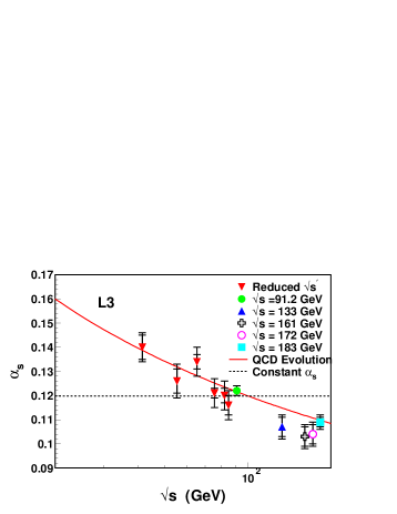
Figure 11: $\alpha_{s}$ measurements from L3 data as a function of $E_{cm}$. The solid and dashed lines represent fits with an energy evolution as predicted by QCD and with constant $\alpha_{s}$, respectively.

Within the L3 analysis[19] the running of $\alpha_{s}$ has been studied including also $\mbox{e}^{+}\mbox{e}^{-}$ annihilation data at reduced center of mass energies $E_{cm}<M_{z}$. For this purpose, events with hard, isolated photons have been selected. This high energy photons are radiated either through initial state radiation or through quark bremsstrahlung, which takes place before the evolution of the hadronic shower. The QCD scale is assumed to be the center of mass energy of the recoiling hadronic system $\sqrt{s^{{}^{\prime}}}$, which is related to the photon energy $E_{\gamma}$ by

$$\sqrt{s^{{}^{\prime}}}=\sqrt{s\left(1-\frac{2E_{\gamma}}{\sqrt{s}}\right)}$$ (11)

The selection provides $\alpha_{s}$ determinations at reduced $\sqrt{s^{{}^{\prime}}}$ from 30 to 86  GeV. $\alpha_{s}$ has been determined from a QCD fit in matched $\cal O$($\alpha_{s}^{2}$) and NLLA precision to the distributions of thrust, heavy jet mass, wide and total jet broadening. Hadronization corrections have been calculated by the means of MC models. Although the matched predictions turned out to be less reliable[1] for the determination of an absolute value for $\alpha_{s}(M_{Z}^{2})$, this should be no problem in terms of the running of the strong coupling, since the errors are fully correlated. Fig. 11 shows the $\alpha_{s}(M_{Z}^{2})$ values measured as a function of $E_{cm}$ together with a fit to the QCD evolution equation. The fit yields a $\chi^{2}$ of 16.9 for 10 degrees of freedom, corresponding to a confidence level of 0.076, whereas a model with constant $\alpha_{s}$ yields a $\chi^{2}$ of 91.4 corresponding to a confidence level of $2.9\times 10^{-13}$.

5 Status of the Strong Coupling

Measurements of the strong coupling are available from a large number of different reactions. Some problems arise, when the individual results are combined in order to calculate a global average. First, a global average of $\alpha_{s}(M_{Z}^{2})$ contains a certain subjective element in the way the input data are selected. There are for example a large number of measurements in $\mbox{e}^{+}\mbox{e}^{-}$ annihilation at different center of mass energies which are however expected to be strongly correlated. The fact, that the exact correlation pattern between different measurements is unknown suggests a pre-clustering of the input data in order to achieve a balanced mixture of measurements from different reaction types, which are then hopefully less correlated. Further problems arise due to the dominance of theoretical uncertainties within the $\alpha_{s}$ determinations. Most experiments try to calculate uncertainties due to missing higher order contributions by the means of the variation of the renormalization scale, however, the range within the scale should be varied is quite arbitrary and different for each experiment. Therefore the resulting uncertainties on $\alpha_{s}(M_{Z}^{2})$ are arbitrary to a large extent as well.

Therefore, three different numbers will be given within the following considerations. The first number is a simple unweighted mean, which has within this context the advantage to ignore the doubtful scale ambiguity errors at all, however, different experimental uncertainties are ignored as well. The second number will be a simple weighted average, which does not account for the (unknown) correlations between the different $\alpha_{s}$ measurements. Also an estimate for a correlated weighted average as introduced in[20] will be given. This method tries to estimate the covariance matrix by assuming a common correlation between the measurements, described by a single parameter $\rho_{\rm eff}$. The method applies, if $\chi^{2}<n_{df}$. Then, the measurements are assumed to be correlated and $\rho_{\rm eff}$ is adjusted until the expectation $\chi^{2}=n_{df}$ is satisfied. In general, this method yields a conservative error estimate. The uncertainty of the average value might be quite large, if (e.g. theoretical) uncertainties are overestimated for some of the measurements included. Too small errors for the individual measurements yield in an underestimation of the correlation between the measurements.

5.1 Status of $\alpha_{s}$ (early 1995)

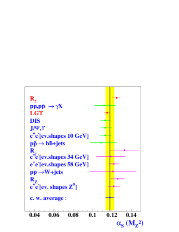
Figure 12: Summary of $\alpha_{s}(M_{Z}^{2})$ measurements at the beginning of 1995[21]. The measurements are ordered according to the energy of the process. The shaded band represents the uncertainty of the correlated weighted average.

value	$\alpha_{s}(M_{Z}^{2})$	$\chi^{2}/n_{df}$
simple mean	$0.1185\pm 0.0072$
simple weighted average	$0.1180\pm 0.0022$	6.4 / 10
correlated w. average	$0.1180\pm 0.0045$

Table 6: A global average for $\alpha_{s}(M_{Z}^{2})$ measurements representing the status in early 1995, estimated using three different methods.

In order to illustrate the enormous progress achieved within the last three years, this overview is started with a summary of $\alpha_{s}(M_{Z}^{2})$ measurements[21] from 1995. Fig. 12 shows a graphical overview of the different measurements. There were apparently two problems with the measurements shown. First the $\alpha_{s}$ measurements from Lattice Gauge Theory (LGT) ( $\alpha_{s}(M_{Z}^{2})$ $=0.115\pm 0.003)$ and from hadronic $\tau$-decays ( $\alpha_{s}(M_{Z}^{2})$ $=0.125\pm 0.004)$, which claimed both to be the most precise, yielded a large difference. They have been ignored in the global average, motivated by the fact that the LGT value has been unstable in the past and the $\tau$-decay value due to the controversial discussion about the validity of some specific theoretical assumptions. The second problem was, that the $\alpha_{s}(M_{Z}^{2})$ values were clustered into two different groups of low and high energy ($Q\gtrsim 25\>\mbox{Ge\kern-0.43057ptV}$) measurements (with the exception of $\alpha_{s}(M_{Z}^{2})$ from $\tau$-decays). The difference observed gave some input for speculations about new physics occurring at this energy scale. The overall scatter of the individual measurements is quite large (see table 6), the uncertainty calculated from a simple weighted average clearly underestimates the true uncertainty, however the correlated weighted average seems to be appropriate here.

5.2 Status of $\alpha_{s}$ today

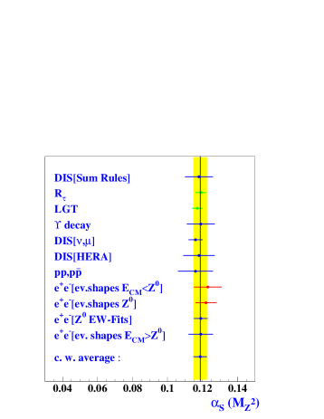
Figure 13: Summary of $\alpha_{s}(M_{Z}^{2})$ measurements. Status after the ICHEP’98 conference.

value	$\alpha_{s}(M_{Z}^{2})$	$\chi^{2}/n_{df}$
simple mean	$0.1187\pm 0.0022$
simple weighted average	$0.1189\pm 0.0014$	1.84 / 10
correlated w. average	$0.1189\pm 0.0039$

Table 7: A global average for $\alpha_{s}(M_{Z}^{2})$ measurements representing the status after the ICHEP’98 conference. The light shaded band represents the uncertainty of the correlated weighted average.

In comparison with 1995 the situation now has drastically changed (see Fig. 13 for a graphical overview on current $\alpha_{s}$ measurements). The difference between $\alpha_{s}(M_{Z}^{2})$ from LGT and from hadronic $\tau$ decays has been largely reduced. Since the $\alpha_{s}(M_{Z}^{2})$ measurements from $\tau$ decays revealed a somewhat larger uncertainty due to the differences from the models employed, a preliminary average of $\alpha_{s}(M_{Z}^{2})$ $=0.119\pm 0.003$ has been considered, corresponding to an average over the three different models introduced before. The current PDG average value for $\alpha_{s}(M_{Z}^{2})$ from LGT of $\alpha_{s}(M_{Z}^{2})$ $=0.117\pm 0.003$[22] is in good agreement with the value from $\tau$ decays and there is no longer a reason to exclude them from the global average. Furthermore, the two clusters of $\alpha_{s}$ values observed earlier completely disappeared. The global average for $\alpha_{s}(M_{Z}^{2})$ (see table 7 ) is nearly the same than in 1995, however the scatter between the individual measurements is largely reduced. The $\chi^{2}$ is 1.84 for 10 degrees of freedom, indicating that the (theoretical) uncertainties might be overestimated. However, the procedure for calculating a correlated weighted average interprets the small $\chi^{2}$ entirely in terms of correlations between the observables, therefore yielding a quite conservative error estimate. The largest deviation from the global average comes from the event shape measurements in $\mbox{e}^{+}\mbox{e}^{-}$ annihilation. Here, the results from matched $\cal O$($\alpha_{s}^{2}$) and NLLA predictions in combination with MC corrections have been used for the global average, since this is the standard method nowadays and a large number of measurements have been made. But as we have seen within the previous discussion, there are serious arguments, why this predictions yield less precise results than predictions in $\cal O$($\alpha_{s}^{2}$) in combination with experimentally optimized scales. It is quite instructive to study the changes on the global average value, when the results from matched predictions are replaced. This will be done in the next section.

5.3 looking into the future …

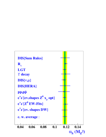
Figure 14: Another summary of $\alpha_{s}(M_{Z}^{2})$ measurements. Here the results from matched $\cal O$($\alpha_{s}^{2}$) and NLLA predictions have been replaced with results from $\cal O$($\alpha_{s}^{2}$) QCD applying experimentally optimized scales, and with results from using DW-model corrections. The light shaded band represents the uncertainty of the correlated weighted average. Additionally the uncertainty of the simple weighted average is indicated by the dark shaded band.

value	$\alpha_{s}(M_{Z}^{2})$	$\chi^{2}/n_{df}$
simple mean	$0.1185\pm 0.0072$
simple weighted average	$0.1180\pm 0.0022$	6.4 / 10
correlated w. average	$0.1180\pm 0.0045$

Table 8: A modified global average for $\alpha_{s}(M_{Z}^{2})$ where the results from matched predictions have been replaced.

In a first step, the global results from $\rm Z^{0}$ data have been replaced by the single result of $\alpha_{s}(M_{Z}^{2})$ $=0.117\pm 0.003$ from the DELPHI collaboration[1], obtained from $\cal O$($\alpha_{s}^{2}$) predictions in combination with experimentally optimized scales. Secondly, it has been assumed, that the DW-model gets established and the results from $\mbox{e}^{+}\mbox{e}^{-}$ data with $E_{cm}\neq M_{Z}$ have been replaced by an average value of current results from DW-model predictions. This average has been calculated assuming fully correlated errors which yields $\alpha_{s}(M_{Z}^{2})$ $=0.117\pm 0.005$. (Here, the results of [15] have been ignored, since only statistical errors are given.) See Fig. 14 for a graphical view and table 8 for the average value. The modified result is quite impressive. The global average is about 1 % smaller than before, and the consistency of the measurements gets further improved. The scatter of the individual measurements is now only $\pm 0.0012$ and the uncertainty of $\Delta\alpha_{s}(M_{Z}^{2})$ $=\pm 0.0038$ seems now really be too pessimistic. The uncertainty obtained from a simple weighted average is about 1 % and indicated in Fig. 14 for illustration reasons. Clearly, no correlations between the measurements are considered here. Also the new results introduced here have to be established. However, if one considers the progress achieved within the last three years, a 1% error on $\alpha_{s}(M_{Z}^{2})$ seems to be a realistic perspective for the foreseeable future.

6 Summary

An enormous progress has been achieved on the determination of $\alpha_{s}(M_{Z}^{2})$ and its running with the analyses presented at this years summer conferences. The importance of adjusting the renormalization scale has been demonstrated with the analysis of high statistics and high precision $\rm Z^{0}$ data using angular dependent shape observables. The observation is confirmed by the analysis of higher moments of event shapes from LEP high energy data. Comparison of the data with predictions from matched $\cal O$($\alpha_{s}^{2}$) with NLLA precision revealed an so far unreported problem, presumably arising due to a mismatch of the renormalization scales. The DW-model is a novel way in understanding non-perturbative power corrections to event shape distributions. First results are impressive. Applying the DW-model, QCD predictions in $\cal O$($\alpha_{s}^{2}$) precision and matched $\cal O$($\alpha_{s}^{2}$) and NLLA precision yield similar $\alpha_{s}(M_{Z}^{2})$ values, which are also in good agreement with other results from precise $\alpha_{s}(M_{Z}^{2})$ measurements. If hadronization corrections from MC models are applied instead, a larger deviation of $\alpha_{s}(M_{Z}^{2})$ is observed for matched predictions, however still compatible with the global $\alpha_{s}(M_{Z}^{2})$ average value. The running of $\alpha_{s}$ is clearly established from LEP $\mbox{e}^{+}\mbox{e}^{-}$ data only. All recent precise $\alpha_{s}(M_{Z}^{2})$ measurements agree very well with each other, a global average of

$\alpha_{s}(M_{Z}^{2})$ $=0.1189\pm 0.0039$

has been determined using a correlated weighted average. Replacing the results from matched $\cal O$($\alpha_{s}^{2}$) and NLLA predictions with the new results obtained from applying experimentally optimized scales and from DW model predictions further improves the consistency of the global $\alpha_{s}(M_{Z}^{2})$ measurements. A roughly 1 % error on $\alpha_{s}(M_{Z}^{2})$ seems to be a realistic perspective for the foreseeable future.

References

-
[1]
DELPHI Collab., S. Hahn and J. Drees, ICHEP’98 #142 (1998),
Paper contributed to the ICHEP’98 in Vancouver and references therein. - [2] M. Seymour, program EVENT2, URL: http://wwwinfo.cern.ch/seymour/nlo.
- [3] E. B. Zijlstra and W. L. van Neerven, Nucl. Phys. B 383 (1992) 525.
- [4] Y. Ohnishi and H. Masuda, SLAC-PUB-6560 (1994).
- [5] M. Grünewald, Talk presented at the ICHEP’98 in Vancouver.
- [6] OPAL Collab., K. Ackerstaff et al., CERN-EP/98-102 (1998).
- [7] ALEPH collab., R. Barate et al., Eur. Phys. Jour. C 4 (1998) 409.
- [8] T.G. Steele and V. Elias, hep-ph/9808490 (1998).
- [9] A.C. Mattingly and P.M. Stevenson, Phys. Rev. D 49 (1994) 439.
- [10] J. Yu, Talk presented at the ICHEP’98 in Vancouver.
-
[11]
T. Doyle, Talk presented at the ICHEP’98 in Vancouver;
W.G. Seligman et al., hep-ex/9701017 (1998). - [12] M. Virchaux and A. Milsztajn, Phys. Lett. B 274 (1992) 221.
-
[13]
Yu.L. Dokshitzer, B.R. Webber, Phys. Lett. B 352 (1995) 451;
Yu.L. Dokshitzer, B.R. Webber, Phys. Lett. B 404 (1997) 321. -
[14]
DELPHI collab., D. Wicke et al., ICHEP’98 #137 (1998)
Paper contributed to the ICHEP’98 in Vancouver. - [15] P.A.M. Fernández, Talk presented at the QCD’98 in Montpellier.
- [16] Yu.L. Dokshitzer, Talk presented at the ICHEP’98 in Vancouver.
-
[17]
ALEPH Collab., ICHEP’98 #940 (1998),
Paper contributed to the ICHEP’98 in Vancouver. -
[18]
OPAL collab., ICHEP’98 #305 (1998),
Paper contributed to the ICHEP’98 in Vancouver. -
[19]
L3 collab., ICHEP’98 #536 (1998),
Paper contributed to the ICHEP’98 in Vancouver. - [20] M. Schmelling, Phys. Scripta 51 (1995) 676.
- [21] M. Schmelling, Phys. Scripta 51 (1995) 683.
- [22] Particle Data Group, C. Caso et al., Europ. Phys. Jour. C 3 (1998) 1