EUROPEAN LABORATORY FOR PARTICLE PHYSICS

CERN-EP/98-186

25 November 1998

A Measurement of
the Product Branching Ratio
$\boldsymbol{f(\mathrm{b}\rightarrow\Lambda_{\mathrm{b}})\cdot\mathrm{BR}(\Lambda_{\mathrm{b}}\rightarrow\Lambda\mathrm{X})}$
in $\boldsymbol{\mathrm{Z}^{0}}$ Decays

The OPAL Collaboration

The product branching ratio, $f(\mathrm{b}\rightarrow\Lambda_{\mathrm{b}})\cdot\mathrm{BR}(\Lambda_{\mathrm{b}}\rightarrow\Lambda\mathrm{X})$, where $\Lambda_{\mathrm{b}}$ denotes any weakly-decaying b–baryon, has been measured using the OPAL detector at LEP. $\Lambda_{\mathrm{b}}$’s are selected by the presence of energetic $\Lambda$ particles in bottom events tagged by the presence of displaced secondary vertices. A fit to the momenta of the $\Lambda$ particles separates signal from B meson and fragmentation backgrounds. The measured product branching ratio is

$$f(\mathrm{b}\rightarrow\Lambda_{\mathrm{b}})\cdot\mathrm{BR}(\Lambda_{\mathrm{b}}\rightarrow\Lambda\mathrm{X})=(2.67\pm 0.38(stat)^{+0.67}_{-0.60}(sys))\%.$$

Combined with a previous OPAL measurement, one obtains

$$f(\mathrm{b}\rightarrow\Lambda_{\mathrm{b}})\cdot\mathrm{BR}(\Lambda_{\mathrm{b}}\rightarrow\Lambda\mathrm{X})=(3.50\pm 0.32(stat)\pm 0.35(sys))\%.$$

(Submitted to the European Physical Journal C)

G. Abbiendi², K. Ackerstaff⁸, G. Alexander²³, J. Allison¹⁶, N. Altekamp⁵, K.J. Anderson⁹, S. Anderson¹², S. Arcelli¹⁷, S. Asai²⁴, S.F. Ashby¹, D. Axen²⁹, G. Azuelos^18,a, A.H. Ball¹⁷, E. Barberio⁸, R.J. Barlow¹⁶, R. Bartoldus³, J.R. Batley⁵, S. Baumann³, J. Bechtluft¹⁴, T. Behnke²⁷, K.W. Bell²⁰, G. Bella²³, A. Bellerive⁹, S. Bentvelsen⁸, S. Bethke¹⁴, S. Betts¹⁵, O. Biebel¹⁴, A. Biguzzi⁵, S.D. Bird¹⁶, V. Blobel²⁷, I.J. Bloodworth¹, P. Bock¹¹, J. Böhme¹⁴, D. Bonacorsi², M. Boutemeur³⁴, S. Braibant⁸, P. Bright-Thomas¹, L. Brigliadori², R.M. Brown²⁰, H.J. Burckhart⁸, P. Capiluppi², R.K. Carnegie⁶, A.A. Carter¹³, J.R. Carter⁵, C.Y. Chang¹⁷, D.G. Charlton^1,b, D. Chrisman⁴, C. Ciocca², P.E.L. Clarke¹⁵, E. Clay¹⁵, I. Cohen²³, J.E. Conboy¹⁵, O.C. Cooke⁸, C. Couyoumtzelis¹³, R.L. Coxe⁹, M. Cuffiani², S. Dado²², G.M. Dallavalle², C. Darling³¹, R. Davis³⁰, S. De Jong¹², A. de Roeck⁸, P. Dervan¹⁵, K. Desch⁸, B. Dienes^33,d, M.S. Dixit⁷, J. Dubbert³⁴, E. Duchovni²⁶, G. Duckeck³⁴, I.P. Duerdoth¹⁶, D. Eatough¹⁶, P.G. Estabrooks⁶, E. Etzion²³, F. Fabbri², M. Fanti², A.A. Faust³⁰, F. Fiedler²⁷, M. Fierro², I. Fleck⁸, R. Folman²⁶, A. Fürtjes⁸, D.I. Futyan¹⁶, P. Gagnon⁷, J.W. Gary⁴, J. Gascon¹⁸, S.M. Gascon-Shotkin¹⁷, G. Gaycken²⁷, C. Geich-Gimbel³, G. Giacomelli², P. Giacomelli², V. Gibson⁵, W.R. Gibson¹³, D.M. Gingrich^30,a, D. Glenzinski⁹, J. Goldberg²², W. Gorn⁴, C. Grandi², K. Graham²⁸, E. Gross²⁶, J. Grunhaus²³, M. Gruwé²⁷, G.G. Hanson¹², M. Hansroul⁸, M. Hapke¹³, K. Harder²⁷, A. Harel²², C.K. Hargrove⁷, C. Hartmann³, M. Hauschild⁸, C.M. Hawkes¹, R. Hawkings²⁷, R.J. Hemingway⁶, M. Herndon¹⁷, G. Herten¹⁰, R.D. Heuer²⁷, M.D. Hildreth⁸, J.C. Hill⁵, P.R. Hobson²⁵, M. Hoch¹⁸, A. Hocker⁹, K. Hoffman⁸, R.J. Homer¹, A.K. Honma^28,a, D. Horváth^32,c, K.R. Hossain³⁰, R. Howard²⁹, P. Hüntemeyer²⁷, P. Igo-Kemenes¹¹, D.C. Imrie²⁵, K. Ishii²⁴, F.R. Jacob²⁰, A. Jawahery¹⁷, H. Jeremie¹⁸, M. Jimack¹, C.R. Jones⁵, P. Jovanovic¹, T.R. Junk⁶, D. Karlen⁶, V. Kartvelishvili¹⁶, K. Kawagoe²⁴, T. Kawamoto²⁴, P.I. Kayal³⁰, R.K. Keeler²⁸, R.G. Kellogg¹⁷, B.W. Kennedy²⁰, D.H. Kim¹⁹, A. Klier²⁶, S. Kluth⁸, T. Kobayashi²⁴, M. Kobel^3,e, D.S. Koetke⁶, T.P. Kokott³, M. Kolrep¹⁰, S. Komamiya²⁴, R.V. Kowalewski²⁸, T. Kress⁴, P. Krieger⁶, J. von Krogh¹¹, T. Kuhl³, P. Kyberd¹³, G.D. Lafferty¹⁶, H. Landsman²², D. Lanske¹⁴, J. Lauber¹⁵, S.R. Lautenschlager³¹, I. Lawson²⁸, J.G. Layter⁴, D. Lazic²², A.M. Lee³¹, D. Lellouch²⁶, J. Letts¹², L. Levinson²⁶, R. Liebisch¹¹, B. List⁸, C. Littlewood⁵, A.W. Lloyd¹, S.L. Lloyd¹³, F.K. Loebinger¹⁶, G.D. Long²⁸, M.J. Losty⁷, J. Ludwig¹⁰, D. Liu¹², A. Macchiolo², A. Macpherson³⁰, W. Mader³, M. Mannelli⁸, S. Marcellini², C. Markopoulos¹³, A.J. Martin¹³, J.P. Martin¹⁸, G. Martinez¹⁷, T. Mashimo²⁴, P. Mättig²⁶, W.J. McDonald³⁰, J. McKenna²⁹, E.A. Mckigney¹⁵, T.J. McMahon¹, R.A. McPherson²⁸, F. Meijers⁸, S. Menke³, F.S. Merritt⁹, H. Mes⁷, J. Meyer²⁷, A. Michelini², S. Mihara²⁴, G. Mikenberg²⁶, D.J. Miller¹⁵, R. Mir²⁶, W. Mohr¹⁰, A. Montanari², T. Mori²⁴, K. Nagai⁸, I. Nakamura²⁴, H.A. Neal¹², B. Nellen³, R. Nisius⁸, S.W. O’Neale¹, F.G. Oakham⁷, F. Odorici², H.O. Ogren¹², M.J. Oreglia⁹, S. Orito²⁴, J. Pálinkás^33,d, G. Pásztor³², J.R. Pater¹⁶, G.N. Patrick²⁰, J. Patt¹⁰, R. Perez-Ochoa⁸, S. Petzold²⁷, P. Pfeifenschneider¹⁴, J.E. Pilcher⁹, J. Pinfold³⁰, D.E. Plane⁸, P. Poffenberger²⁸, J. Polok⁸, M. Przybycień⁸, C. Rembser⁸, H. Rick⁸, S. Robertson²⁸, S.A. Robins²², N. Rodning³⁰, J.M. Roney²⁸, K. Roscoe¹⁶, A.M. Rossi², Y. Rozen²², K. Runge¹⁰, O. Runolfsson⁸, D.R. Rust¹², K. Sachs¹⁰, T. Saeki²⁴, O. Sahr³⁴, W.M. Sang²⁵, E.K.G. Sarkisyan²³, C. Sbarra²⁹, A.D. Schaile³⁴, O. Schaile³⁴, F. Scharf³, P. Scharff-Hansen⁸, J. Schieck¹¹, B. Schmitt⁸, S. Schmitt¹¹, A. Schöning⁸, M. Schröder⁸, M. Schumacher³, C. Schwick⁸, W.G. Scott²⁰, R. Seuster¹⁴, T.G. Shears⁸, B.C. Shen⁴, C.H. Shepherd-Themistocleous⁸, P. Sherwood¹⁵, G.P. Siroli², A. Sittler²⁷, A. Skuja¹⁷, A.M. Smith⁸, G.A. Snow¹⁷, R. Sobie²⁸, S. Söldner-Rembold¹⁰, S. Spagnolo²⁰, M. Sproston²⁰, A. Stahl³, K. Stephens¹⁶, J. Steuerer²⁷, K. Stoll¹⁰, D. Strom¹⁹, R. Ströhmer³⁴, B. Surrow⁸, S.D. Talbot¹, S. Tanaka²⁴, P. Taras¹⁸, S. Tarem²², R. Teuscher⁸, M. Thiergen¹⁰, J. Thomas¹⁵, M.A. Thomson⁸, E. von Törne³, E. Torrence⁸, S. Towers⁶, I. Trigger¹⁸, Z. Trócsányi³³, E. Tsur²³, A.S. Turcot⁹, M.F. Turner-Watson¹, I. Ueda²⁴, R. Van Kooten¹², P. Vannerem¹⁰, M. Verzocchi¹⁰, H. Voss³, F. Wäckerle¹⁰, A. Wagner²⁷, C.P. Ward⁵, D.R. Ward⁵, P.M. Watkins¹, A.T. Watson¹, N.K. Watson¹, P.S. Wells⁸, N. Wermes³, J.S. White⁶, G.W. Wilson¹⁶, J.A. Wilson¹, T.R. Wyatt¹⁶, S. Yamashita²⁴, G. Yekutieli²⁶, V. Zacek¹⁸, D. Zer-Zion⁸

¹School of Physics and Astronomy, University of Birmingham, Birmingham B15 2TT, UK
²Dipartimento di Fisica dell’ Università di Bologna and INFN, I-40126 Bologna, Italy
³Physikalisches Institut, Universität Bonn, D-53115 Bonn, Germany
⁴Department of Physics, University of California, Riverside CA 92521, USA
⁵Cavendish Laboratory, Cambridge CB3 0HE, UK
⁶Ottawa-Carleton Institute for Physics, Department of Physics, Carleton University, Ottawa, Ontario K1S 5B6, Canada
⁷Centre for Research in Particle Physics, Carleton University, Ottawa, Ontario K1S 5B6, Canada
⁸CERN, European Organisation for Particle Physics, CH-1211 Geneva 23, Switzerland
⁹Enrico Fermi Institute and Department of Physics, University of Chicago, Chicago IL 60637, USA
¹⁰Fakultät für Physik, Albert Ludwigs Universität, D-79104 Freiburg, Germany
¹¹Physikalisches Institut, Universität Heidelberg, D-69120 Heidelberg, Germany
¹²Indiana University, Department of Physics, Swain Hall West 117, Bloomington IN 47405, USA
¹³Queen Mary and Westfield College, University of London, London E1 4NS, UK
¹⁴Technische Hochschule Aachen, III Physikalisches Institut, Sommerfeldstrasse 26-28, D-52056 Aachen, Germany
¹⁵University College London, London WC1E 6BT, UK
¹⁶Department of Physics, Schuster Laboratory, The University, Manchester M13 9PL, UK
¹⁷Department of Physics, University of Maryland, College Park, MD 20742, USA
¹⁸Laboratoire de Physique Nucléaire, Université de Montréal, Montréal, Quebec H3C 3J7, Canada
¹⁹University of Oregon, Department of Physics, Eugene OR 97403, USA
²⁰CLRC Rutherford Appleton Laboratory, Chilton, Didcot, Oxfordshire OX11 0QX, UK
²²Department of Physics, Technion-Israel Institute of Technology, Haifa 32000, Israel
²³Department of Physics and Astronomy, Tel Aviv University, Tel Aviv 69978, Israel
²⁴International Centre for Elementary Particle Physics and Department of Physics, University of Tokyo, Tokyo 113-0033, and Kobe University, Kobe 657-8501, Japan
²⁵Institute of Physical and Environmental Sciences, Brunel University, Uxbridge, Middlesex UB8 3PH, UK
²⁶Particle Physics Department, Weizmann Institute of Science, Rehovot 76100, Israel
²⁷Universität Hamburg/DESY, II Institut für Experimental Physik, Notkestrasse 85, D-22607 Hamburg, Germany
²⁸University of Victoria, Department of Physics, P O Box 3055, Victoria BC V8W 3P6, Canada
²⁹University of British Columbia, Department of Physics, Vancouver BC V6T 1Z1, Canada
³⁰University of Alberta, Department of Physics, Edmonton AB T6G 2J1, Canada
³¹Duke University, Dept of Physics, Durham, NC 27708-0305, USA
³²Research Institute for Particle and Nuclear Physics, H-1525 Budapest, P O Box 49, Hungary
³³Institute of Nuclear Research, H-4001 Debrecen, P O Box 51, Hungary
³⁴Ludwigs-Maximilians-Universität München, Sektion Physik, Am Coulombwall 1, D-85748 Garching, Germany

^a and at TRIUMF, Vancouver, Canada V6T 2A3
^b and Royal Society University Research Fellow
^c and Institute of Nuclear Research, Debrecen, Hungary
^d and Department of Experimental Physics, Lajos Kossuth University, Debrecen, Hungary
^e on leave of absence from the University of Freiburg

1 Introduction

In this paper, we present a measurement of the product branching ratio, $f(\mathrm{b}\rightarrow\Lambda_{\mathrm{b}})\cdot\mathrm{BR}(\Lambda_{\mathrm{b}}\rightarrow\Lambda\mathrm{X})$, at the $\mathrm{Z}^{0}$ resonance. In this process a b quark from $\mathrm{Z}^{0}\rightarrow\mathrm{b\bar{b}}$ decays produces a b-flavoured baryon which decays, directly or indirectly, into a $\Lambda$ baryon and other particles. Previous studies of inclusive b–baryon decays have emphasized semileptonic decays of the $\Lambda_{\mathrm{b}}$[1, 2, 3].

The result presented here, when combined with the semileptonic branching ratio, $f(\mathrm{b}\rightarrow\Lambda_{\mathrm{b}})\cdot\mathrm{BR}(\Lambda_{\mathrm{b}}\rightarrow\Lambda\ell\mathrm{X})$, allows one to determine the ratio $\Gamma(\Lambda_{\mathrm{b}}\rightarrow\Lambda\ell\mathrm{X})/\Gamma(\Lambda_{\mathrm{b}}\rightarrow\Lambda\mathrm{X})$[4]. Since $\Gamma(\Lambda_{\mathrm{b}}\rightarrow\Lambda\ell\mathrm{X})$ depends on $\mathrm{V_{cb}}$ and well understood leptonic currents, it may also be possible to extract this fundamental weak parameter in a setting with hadronic uncertainties different from those of B meson measurements [5, 6].

For this analysis, we select events containing a $\Lambda$ particle and a vertex significantly displaced from the $\mathrm{Z}^{0}$ decay point. This gives a sample enriched in $\Lambda_{\mathrm{b}}$’s. Significant backgrounds come from the decay of B mesons into $\Lambda$ particles, and from b-hadron events where a high-momentum $\Lambda$ is produced in the primary hadronisation process. These backgrounds are separated from the signal by using a simultaneous fit to the momentum and transverse momentum distributions of the $\Lambda$ baryon.

The previously published OPAL measurement of the product branching ratio used a “companion baryon technique” to identify jets containing a $\Lambda_{\mathrm{b}}$[4]. That analysis used the momenta of a $\Lambda$ and an anti-baryon identified in the same hemisphere, whereas this analysis uses the momentum and transverse momentum of a $\Lambda$. The two techniques are complementary and have less than 20% of events in common.

After general information about the OPAL detector and Monte Carlo event simulation, we outline the event selection which provides an enriched sample of $\Lambda_{\mathrm{b}}$. The backgrounds are then addressed, followed by a discussion of signal efficiencies. Systematic errors are discussed in detail. Finally, the measured value of the product branching ratio is presented. This is combined with the previous OPAL measurement, and is used to update the ratio $\mathrm{BR}(\Lambda_{\mathrm{b}}\rightarrow\Lambda\ell\mathrm{X})/\mathrm{BR}(\Lambda_{\mathrm{b}}\rightarrow\Lambda\mathrm{X})$ from [4].

2 The OPAL Detector and Its Simulation

The OPAL detector is described in detail elsewhere [7]. Here, we briefly describe the components which are particularly relevant to this analysis. Charged particle tracking is performed by the central tracking system which is located in a solenoidal magnetic field of 0.435 T. The central tracking system consists of a two-layer silicon micro-vertex detector [8], a high-precision vertex drift chamber, a large-volume jet chamber and $z$–chambers for accurately measuring track coordinates along the beam direction.

The measurement of specific ionisation in the jet chamber, ${\mathrm{d}E}/{\mathrm{d}x}$, is used for particle identification. Tracks emitted at large angle to the beam direction have up to 159 samplings providing a ${\mathrm{d}E}/{\mathrm{d}x}$ resolution of 3.2% [9].

The central detector is surrounded by a lead-glass electromagnetic calorimeter with a wire streamer chamber as presampler. The iron magnet yoke is instrumented with layers of streamer tubes which serve as a hadron calorimeter and provide information for muon identification. Four layers of planar drift chambers surround the hadron calorimeter and serve for tracking muons.

To obtain momentum distributions of $\Lambda$’s from different sources, and to evaluate efficiencies and backgrounds, we utilize 6 million $\mathrm{Z}^{0}\rightarrow\mathrm{q\bar{q}}$ and 3 million $\mathrm{Z}^{0}\rightarrow\mathrm{b\bar{b}}$ simulated events. The Monte Carlo simulation of the OPAL detector is described elsewhere [10]. The JETSET 7.4 string fragmentation program is used to form hadrons and decay short-lived particles [11, 12]. The fragmentation function of Peterson et al., is used for heavy flavors, ($\epsilon_{P}=0.0038$ for b quarks) [13, 14]. For this analysis the $\Lambda$ momentum in the rest frame of B mesons for $\Lambda$’s from B meson decay is tuned to match measurements by CLEO [15].

3 Event Selection

This study uses a total of 3 554 212 hadronic $\mathrm{Z}^{0}$ decays collected by the OPAL detector between 1991 and 1995. The method for selecting hadronic $\mathrm{Z}^{0}$ decays has been described in previous OPAL publications [16, 17] and has an efficiency of $(98.7\pm 0.4)\%$.

To select events with a clear two-jet structure, the thrust of the event is required to be at least $0.8$ [18]. Events are also required to be in that region of the detector with good ${\mathrm{d}E}/{\mathrm{d}x}$ and silicon micro-vertex coverage by requiring $\left|\cos(\theta_{T})\right|<0.75$, where $\theta_{T}$ is the polar angle of the thrust axis. After the angular acceptance cut, thrust cut, and requiring important detector components to be operational, $\mathrm{N_{mh}}$ = 2 323 302 multihadronic events are retained.

Reconstructed vertices displaced from the interaction point are used to select $\mathrm{Z}^{0}\rightarrow\mathrm{b\bar{b}}$ events. The primary vertex is determined for each event using the average beam spot position as a constraint [19, 20]. Jets are found using a cone algorithm with a cone having a half-angle of 0.55 radians and a minimum jet energy of 5.0 GeV [21]. Both charged tracks and calorimeter clusters not associated with a track are used to identify jets. An iterative approach is used when attempting to form a significantly displaced vertex, referred to as a secondary vertex, in each jet [22]. Events containing at least one reconstructed secondary vertex are retained. The efficiency of tagging a jet associated with a b quark is measured to be $(21.2\pm 0.9)\%$ for a purity of $(95.5\pm 0.5)\%$. Details of the efficiency calculation are described in section 7.

4 $\boldsymbol{\Lambda}$ Identification

Events are split into hemispheres using the plane orthogonal to the thrust axis. $\Lambda$ particles are identified both in the hemisphere with a jet containing a secondary vertex and in the opposite hemisphere to increase the sample size.

The $\Lambda$ selection used here is similar to the method described in [12]. $\Lambda$’s are reconstructed via the decay $\Lambda\rightarrow\mathrm{p}\pi$. All combinations of well–measured oppositely-charged tracks forming a vertex are considered. The higher momentum track is assumed to be the proton. Each track is required to have a significant impact parameter in the r-$\phi$ plane with respect to the primary vertex to reduce combinatorial backgrounds. The $\Lambda$ direction is required to be in the range $|\cos(\theta)_{\Lambda}|<0.9$. The momentum component parallel to the beam line for each track, $p_{z}$, is re-calculated assuming it originates from the reconstructed $\Lambda$ decay point [2]. $\Lambda$ candidates whose invariant mass lies within 8 $\mathrm{MeV/c}^{2}$ of the nominal $\Lambda$ mass are accepted if the invariant mass, assuming pion masses for both tracks, does not fall within 6 $\mathrm{MeV/c}^{2}$ of the $\mathrm{K_{s}^{0}}$ mass.

The ${\mathrm{d}E}/{\mathrm{d}x}$ identification of the candidate proton requires that the observed energy loss is consistent with a proton and inconsistent with that of a pion of the same momentum. No ${\mathrm{d}E}/{\mathrm{d}x}$ requirements are made on the pion candidate.

The reconstructed decay point of the $\Lambda$ is required to be at a distance greater than 8 cm in the r-$\phi$ plane from the primary interaction point. There must be no hits in the silicon detector that are associated with either of the tracks. The angle $\phi(\Lambda)$ between the position vector of the $\Lambda$ decay vertex and its momentum vector is required to be less than 14 mrad. To reduce $\Lambda$’s coming from fragmentation, the opening angle of the $\Lambda$ direction with the jet axis is required to be less than 0.2 radians, and the momentum of the $\Lambda$ is required to be greater than 5 $\mathrm{GeV/c}$.

Monte Carlo studies indicate that the fake $\Lambda$’s remaining in $\mathrm{Z}^{0}\rightarrow\mathrm{b\bar{b}}$ events are predominantly from real $\Lambda$ decays where one decay product of the $\Lambda$ is combined with a random track. The fake $\Lambda$ rate has been studied using side-bands of the $\Lambda$ mass distribution and, for the selection criteria of this paper, is estimated at 2% in both data and Monte Carlo. The above selection retains 1582 events.

5 Backgrounds

Besides the $\Lambda_{\mathrm{b}}\rightarrow\Lambda\mathrm{X}$ signal, the selected event sample contains the following backgrounds: (1) events with a b-hadron and a $\Lambda$ produced in the hadronisation process, (2) $\Lambda$’s from B meson decay, (3) other backgrounds and fake $\Lambda$ baryons. These three background sources are discussed below.

(1) Events where a $\Lambda$ baryon arises in hadronisation can be separated from those produced in $\Lambda_{\mathrm{b}}$ decays on a statistical basis. The $\Lambda$ baryons from this source generally have low momentum, $p$, and transverse momentum, $p_{t}$. There are two distinct sub-classes to this background:

• the $\Lambda$ is created in associated production with another light baryon within a $\mathrm{Z}^{0}\rightarrow\mathrm{b\bar{b}}$ event;

• the $\Lambda$ is created in associated production with a primary b–baryon.

Monte Carlo studies indicate that these two classes of $\Lambda$ baryons have similar $p$ and $p_{t}$ distributions, which are different from those of the signal. Before the minimum momentum cut, the momentum spectrum for fragmentation $\Lambda$’s peaks at 1 GeV, and $p_{t}$ is peaked at 200 MeV. Because these distributions have long tails, it is not possible to remove all fragmentation $\Lambda$’s with a cut.

(2) $\mathrm{B}\rightarrow\Lambda\mathrm{X}$ decays are a significant background. Although the branching ratio for this process is small, the fraction of b quarks which hadronise to B mesons is $(89.9^{+3.1}_{-3.5})\%$ in $\mathrm{Z}^{0}$ decays [14], so the $\Lambda$ yield from B mesons is about the same as that from $\Lambda_{\mathrm{b}}$ baryons. However, $\Lambda$’s from B meson decays have a softer $p_{t}$ spectrum than the signal since baryon number conservation requires an additional baryon in the decay products of the B meson.

While not yet observed, it is expected that the $\mathrm{B^{0}_{s}}$ meson will produce $\Lambda$’s in its decay chain. The kinematics are assumed to be similar to $\mathrm{B^{0}}$ decays. Excited B mesons are also produced in $\mathrm{Z}^{0}\rightarrow\mathrm{b\bar{b}}$ hadronisation. We assume that these mesons decay either hadronically or electromagnetically to a weakly decaying B meson, and that the kinematics are similar to when the B mesons are directly produced in the ground state.

(3) Other backgrounds contribute 3% to the sample. The $\mathrm{D^{+}}$ is the only charmed hadron with a lifetime long enough to produce a signficant background after requiring a displaced vertex. However, since the $\mathrm{D^{+}}$ is too light to decay to a $\Lambda$ and an anti–baryon, it is only a background when coupled with a fragmentation $\Lambda$ or a charm baryon to $\Lambda$ decay in the opposite hemisphere. The few $\mathrm{D^{+}}$ events accepted are included in the background class (1) above, since they are kinematically similar. Leading $\Lambda$ baryons from light quark (u,d,s) decays of the $\mathrm{Z}^{0}$ are less than 1% of the sample due to the secondary vertex requirement.

6 Fitting the $\boldsymbol{\Lambda}$ Momentum and Transverse Momentum Spectra

The fraction of $\Lambda$’s from $\Lambda_{\mathrm{b}}\rightarrow\Lambda\mathrm{X}$ decays is determined by simultaneously fitting the total and transverse momentum spectra of the $\Lambda$ particles. Figure 1 shows the six input Monte Carlo distributions used in the fit. They are the $p$ and $p_{t}$ for $\Lambda$’s from b–baryons and the two backgrounds: B meson and fragmentation. (The uncertainties due to these Monte Carlo distributions are discussed in section 9.) The fit returns the fractions of the signal and the two major backgrounds in the data.

The fit, which takes into account finite statistics, uses a binned maximum likelihood technique described in [23]. The 25% correlation between $p$ and $p_{t}$ is not taken into account by this technique. The effect of correlations was studied using Monte Carlo samples. This technique underestimates the error by 5%, but the central value of the fit fraction is unchanged. We correct the error for this effect.

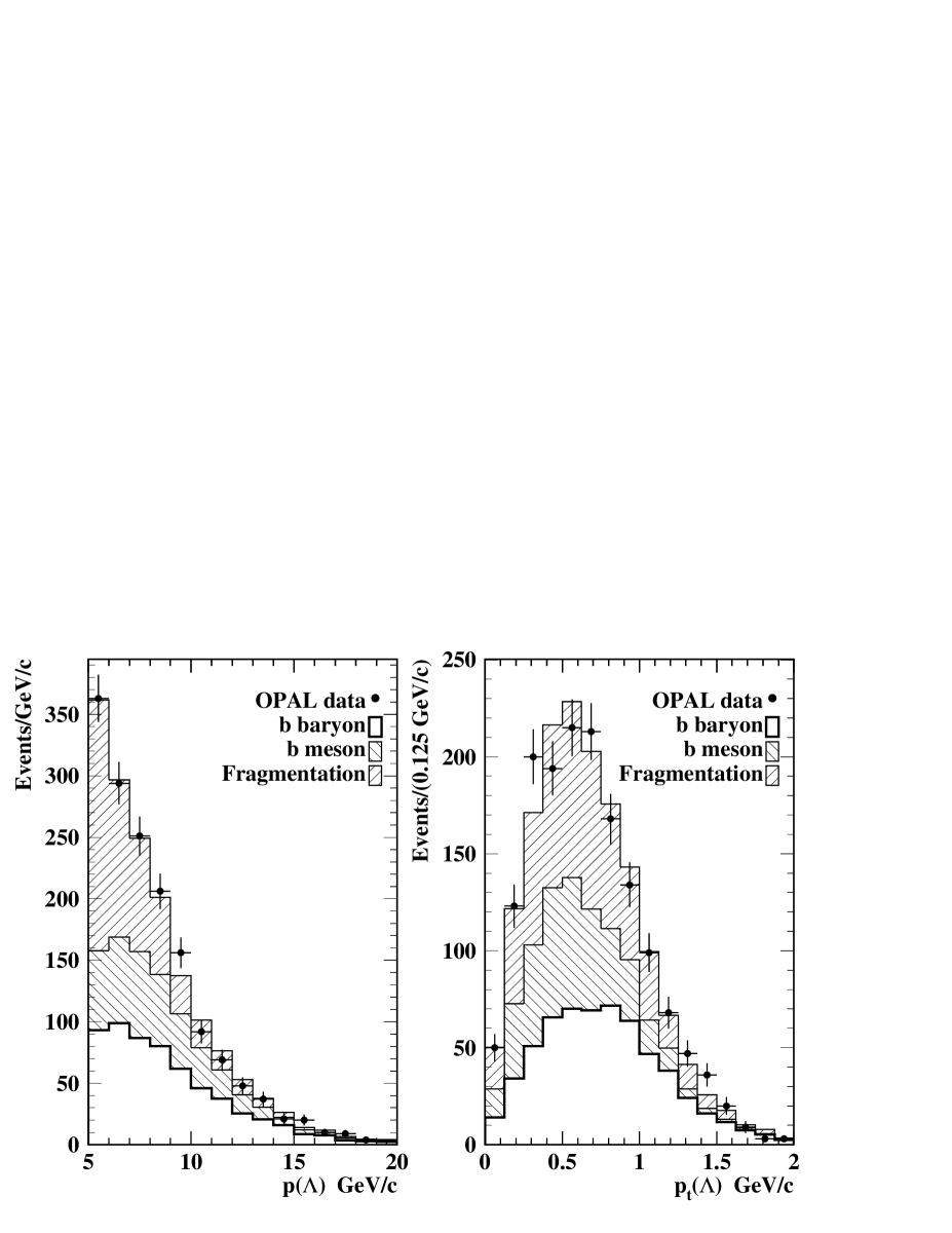
Figure 2: Distributions of $\Lambda$ $p$ and $p_{t}$ in data (points with error bars) and Monte Carlo (histogram). The three sources: fragmentation, B meson, and $\Lambda_{\mathrm{b}}$ are normalized to their fitted fractions.

The fitted distributions are shown in Figure 2 and the fractions are listed in Table 1. The $\chi^{2}$ of the fit is 25 for 27 degrees of freedom. The fraction of signal events is fitted to be ($37.4\pm 5.3$)%, where the error is due to finite statistics in data and Monte Carlo. This corresponds to $592\pm 83$ $\Lambda_{\mathrm{b}}\rightarrow\Lambda\mathrm{X}$ signal events.

The fit method was checked by performing 5000 trial fits on fake data samples which were generated by adding the three Monte Carlo sources and allowing the histogram bins to vary according to Poisson statistics. The distribution of fit fractions matches the values in the fake data with a standard deviation equal to the uncertainty assigned by the fitting routine.

The stability of the fit result was checked by varying the minimum $p$ and $p_{t}$ allowed in the fit and recalculating the product branching ratio for each case. The $\Lambda$ momentum was allowed to vary from 3 $\mathrm{GeV/c}$ to 8 $\mathrm{GeV/c}$ in 1 $\mathrm{GeV/c}$ steps. We also varied the minimum $p_{t}$ cut from 0.0 to 0.75 $\mathrm{GeV/c}$ in 0.25 $\mathrm{GeV/c}$ steps while holding the minimum $p$ cut constant at 5 $\mathrm{GeV/c}$. For all cases the product branching ratio was consistent within $10\%$ and there were no deviations that were not compatible with statistical fluctuations.

Source	Fit fraction (%)	Correlations
		$\Lambda_{\mathrm{b}}\rightarrow\Lambda\mathrm{X}$	$\mathrm{frag}\rightarrow\Lambda\mathrm{X}$	$\mathrm{B}\rightarrow\Lambda\mathrm{X}$
$\Lambda_{\mathrm{b}}\rightarrow\Lambda\mathrm{X}$	37.4 $\pm$ 5.3	1.0	–0.15	–0.64
$\mathrm{frag}\rightarrow\Lambda\mathrm{X}$	37.1 $\pm$ 5.1	–0.15	1.0	–0.61
$\mathrm{B}\rightarrow\Lambda\mathrm{X}$	25.5 $\pm$ 6.6	–0.64	–0.61	1.0

Table 1: Results of the fit. The fit fractions indicate the fraction of each source in the data sample. The correlations between the fit fractions are also shown.

7 Secondary Vertex Reconstruction Efficiency

The overall secondary vertex reconstruction efficiency, $\epsilon_{sig}^{b}$, depends on the efficiency of reconstructing a secondary vertex in both the unbiased b hemisphere, $\epsilon_{\mathrm{b}}$, and the hemisphere containing the decay $\Lambda_{\mathrm{b}}\rightarrow\Lambda\mathrm{X}$, $\epsilon^{b}_{\Lambda_{\mathrm{b}}\rightarrow\Lambda\mathrm{X}}$. To measure the efficiency of reconstructing a secondary vertex in an unbiased b-hadron hemisphere, we compare the fraction of tagged hemispheres in events with at least one reconstructed secondary vertex to the number of events with a reconstructed vertex in both hemispheres. This is done for a sample of multihadron events which pass all selection criteria except $\Lambda$ identification.

Solving the following equations for $\epsilon_{\mathrm{b}}$ yields the efficiency.

$$R_{b}\epsilon_{\mathrm{b}}+R_{udsc}\epsilon_{\mathrm{udsc}}=f_{\mathrm{1v}}$$ (1)

$$R_{b}\epsilon_{\mathrm{b}}^{2}+R_{udsc}\epsilon_{\mathrm{udsc}}^{2}=f_{\mathrm{2v}}$$ (2)

The efficiency of selecting a non-b hemisphere is represented by the symbol $\epsilon_{\mathrm{udsc}}$, $f_{\mathrm{1v}}$ is the fraction of hemispheres with a reconstructed secondary vertex, $f_{\mathrm{2v}}$ is the fraction of events in which both hemispheres have a secondary vertex, $R_{b}$ is $\Gamma_{\mathrm{b\bar{b}}}/\Gamma_{\mathrm{had}}=0.2169$ [14] and $R_{udsc}\ =1-R_{b}$. This measurement yields a value for $\epsilon_{\mathrm{b}}$ of $(21.2\pm 0.9$)%, where the error is from finite statistics in the data and Monte Carlo, and year-by-year variations in the detector configuration. The effect of tagging efficiency correlations between the hemispheres is negligible for this analysis.

The presence of a high-momentum $\Lambda$ in a hemisphere reduces the efficiency for reconstructing a secondary vertex. This is true for all sources of $\Lambda$’s in the sample. The proton and pion from $\Lambda$’s in signal events are unlikely to be included in a secondary vertex, which reduces its probability of being reconstructed. The $\Lambda$ selection enhances the proportion of $\Lambda_{\mathrm{b}}$’s which have a shorter lifetime than the average b-hadron. Monte Carlo studies indicate that, when the average b-hadron lifetime is adjusted to that of the $\Lambda_{\mathrm{b}}$, the shorter lifetime reduces the secondary vertex reconstruction efficiency by a factor of $0.84\pm 0.05$. Lastly, if the selected high momentum $\Lambda$ is from fragmentation, the primary b-hadron will have less momentum than usual. A shorter flight distance decreases the probability of reconstructing a displaced vertex.

To calculate the efficiency for reconstructing secondary vertices in $\Lambda_{\mathrm{b}}\rightarrow\Lambda\mathrm{X}$ hemispheres, we begin by comparing the number of selected $\Lambda$’s in the same hemisphere as a reconstructed secondary vertex (same-side) to the number of $\Lambda$’s in the opposite hemisphere (opposite-side). If the presence of high-momentum $\Lambda$’s had no effect on the reconstruction of vertices we would expect to find the same number of same-side and opposite-side $\Lambda$’s in the sample. Instead, we find that the ratio of same-side to opposite-side $\Lambda$’s is $R^{(data)}=0.58\pm 0.03$ and $R^{(MC)}=0.64\pm 0.01$. In the Monte Carlo the ratios for specific sources of $\Lambda$’s are: $R_{\Lambda_{\mathrm{b}}}^{(MC)}=0.54\pm 0.03$, $R_{frag}^{(MC)}=0.62\pm 0.03$, $R_{Bmeson}^{(MC)}=0.77\pm 0.03$.

$R^{(MC)}$ must be multiplied by a factor of 0.9 to match $R^{(data)}$. Assuming that this factor is the same for each source, the corrected ratio for $\Lambda_{\mathrm{b}}$ is $R^{\prime(data)}_{\Lambda_{\mathrm{b}}}=0.49\pm 0.06$, where the full size of the correction is included in the uncertainty. The efficiency for tagging hemispheres with the decay $\Lambda_{\mathrm{b}}\rightarrow\Lambda\mathrm{X}$ is

$$\epsilon_{\Lambda_{\mathrm{b}}\rightarrow\Lambda\mathrm{X}}^{b}=\epsilon_{\mathrm{b}}\cdot R^{\prime(data)}_{\Lambda_{\mathrm{b}}}=(10.4\pm 1.3)\%$$ (3)

where the error includes both statistical and systematic uncertainties.

An event containing a $\Lambda_{\mathrm{b}}\rightarrow\Lambda\mathrm{X}$ decay may be tagged by a reconstructed secondary vertex either in the hemisphere containing the $\Lambda$ or in the opposite hemisphere. The overall efficiency for identifying displaced vertices in these events is therefore:

$$\epsilon_{sig}^{b}=\epsilon_{\Lambda_{\mathrm{b}}\rightarrow\Lambda\mathrm{X}}^{b}+\epsilon_{\mathrm{b}}(1-\epsilon_{\Lambda_{\mathrm{b}}\rightarrow\Lambda\mathrm{X}}^{b})=(29.4\pm 1.5)\%.$$ (4)

8 $\boldsymbol{\Lambda}$ Reconstruction Efficiency

The efficiency of $\Lambda$ reconstruction is determined from Monte Carlo for $\Lambda$’s satisfying all selection criteria. The Monte Carlo simulates well the kinematic properties like $\Lambda$ mass resolution, momentum distributions, and the ${\mathrm{d}E}/{\mathrm{d}x}$ response of the detector. The overall efficiency for reconstructing $\Lambda$ particles from $\Lambda_{\mathrm{b}}$ decay, $\epsilon_{\Lambda}$, is found to be $(11.7\pm 0.6)\%$ for a minimum momentum of 5 $\mathrm{GeV/c}$. The error comes from Monte Carlo statistics, the 2% fake rate and the tracking resolution. The sensitivity to tracking resolution was studied by varying the Monte Carlo resolutions by $\pm 10\%$ which caused the $\Lambda$ identification efficiency to change by $\pm 0.4\%$.

9 Systematic Uncertainty due to Monte Carlo Distributions

The simultaneous fit to the momentum spectra of the $\Lambda$ candidates requires six Monte Carlo input distributions: the $p$ and $p_{t}$ of $\Lambda$’s from b–baryon, B meson, and fragmentation sources. A systematic error is assigned to account for possible mis-modelling of these distributions. Each distribution is checked against a data sample, though the comparisons are limited because it is impossible to obtain pure, large data samples for the three sources.

This section describes how the uncertainties on each of the Monte Carlo distributions are determined and how they propagate to the fit fraction for the $\Lambda_{\mathrm{b}}$ source, $f_{\Lambda_{\mathrm{b}}}$. The results are summarised in Table 2.

Sources of Systematic Errors for $f_{\Lambda_{\mathrm{b}}}$	negative	positive
	errors	errors
$p$($\Lambda$) and $p_{t}$($\Lambda$) from $\mathrm{B}\rightarrow\Lambda\mathrm{X}$	–3.5%	3.5%
$p$($\Lambda$) of Fragmentation $\Lambda$’s	–1.3%	0.8%
$p_{t}$($\Lambda$) of Fragmentation	–12.5%	12.7%
$p$($\Lambda$) from $\Lambda_{\mathrm{b}}\rightarrow\Lambda\mathrm{X}$	–2.9%	4.8%
$p_{t}$($\Lambda$) from $\Lambda_{\mathrm{b}}\rightarrow\Lambda\mathrm{X}$	–16.6%	19.8%
Tracking Uncertainty	–2.7%	2.7%
Total	–21.5%	24.4%

Table 2: Systematic errors contributing to the uncertainty in the measurement of the $\Lambda_{\mathrm{b}}$ fit fraction, $f_{\Lambda_{\mathrm{b}}}$.

$\boldsymbol{\Lambda}$’s from B mesons

The Monte Carlo momentum spectra of $\Lambda_{\mathrm{c}}$’s and $\Lambda$’s coming from B mesons are adjusted to match CLEO data [15]. In the B meson rest frame, the CLEO data have large errors for $\Lambda$’s with momentum less than 0.5 GeV/c. $\Lambda$’s with low momentum in the rest frame of the B meson are reweighted within a range corresponding to these uncertainties, and the fit is repeated for several reweightings in the selected range, changing the $\Lambda_{\mathrm{b}}$ fit fraction by 7%. Values in the center of the range are used in the final fit, and an error of 3.5%, half of the variation observed, is assigned for the uncertainty in the B meson $p$ and $p_{t}$ distributions.

$\boldsymbol{\Lambda}$’s from Fragmentation

A powerful technique for isolating $\Lambda$’s coming from $\Lambda_{\mathrm{b}}$ baryons requires that a lepton with high momentum and transverse momentum be identified in the hemisphere with the $\Lambda$ [1, 2]. For these studies lepton refers to only electrons and muons. The correlation between lepton charge and baryon number of the $\Lambda$ is indicative of its origin: combinations with opposite lepton charge and baryon number (right-sign) are used to tag $\Lambda_{\mathrm{b}}\rightarrow\Lambda\ell\mathrm{X}$ events; wrong-sign combinations yield a high purity of fragmentation $\Lambda$’s [4], which are used as a control sample to compare the $p$ and $p_{t}$ spectra of fragmentation $\Lambda$’s in the data and Monte Carlo.

The lepton identification of [24] is used. The $\Lambda$ selection is tuned to maximize the number and purity of $\Lambda$’s from fragmentation in the wrong-sign sample. Differences with respect to the event selection of section 4 include removing the secondary vertex requirement and requiring the invariant mass of the $\Lambda$–lepton pair to be greater than 2 $\mathrm{GeV/c^{2}}$ to reject $\Lambda_{\mathrm{c}}$ and B meson decays. With this selection, 266 data events are found with a purity of fragmentation $\Lambda$’s of 75%.

Plots a) and c) of Figure 3 show the comparison of the data and Monte Carlo wrong-sign distributions. The means of the $p$ and $p_{t}$ distributions for data and Monte Carlo agree well and are listed in Table 3. We calculate an uncertainty in the agreement by adding in quadrature the errors on the data and Monte Carlo means. An uncertainty of 2.4% is assigned for the momentum distribution and 4.2% for the transverse momentum distribution.

To assess a systematic error on $f_{\Lambda_{\mathrm{b}}}$ due to the Monte Carlo simulation of $p$ or $p_{t}$, each entry in a distribution is multiplied by a factor which raises or lowers the mean of the distribution. For example, to see the effect of the 2.4% uncertainty on the $p$ mean we multiply each entry by 0.976, which shifts the mean downward. The fit is then repeated with the shifted distribution to observe the change in $f_{\Lambda_{\mathrm{b}}}$. The procedure is repeated with a factor of 1.024 to determine the positive error on $f_{\Lambda_{\mathrm{b}}}$.

The fit fraction $f_{\Lambda_{\mathrm{b}}}$ changes by ${}^{+0.8}_{-1.3}$ % when the fragmentation p distribution is varied by its uncertainty, and by ${}^{+12.7}_{-12.5}$ % when the $p_{t}$ distrubution is varied. These changes are assigned as systematic errors on $f_{\Lambda_{\mathrm{b}}}$ due to uncertainties in the fragmentation $\Lambda$ spectra.

	$\mu_{data}$ ($\mathrm{GeV/c}$)	$\mu_{MC}$ ($\mathrm{GeV/c}$)	$\delta\mu$	$\sigma_{\mu}$
WS $p$($\Lambda$)	7.70 $\pm$ 0.15	7.55 $\pm$ 0.09	2.0%	2.4%
WS $p_{t}$($\Lambda$)	0.70 $\pm$ 0.03	0.67 $\pm$ 0.01	4.0%	4.2%
RS-WS $p$($\Lambda$)	8.63 $\pm$ 0.28	8.84 $\pm$ 0.10	2.4%	3.4%
RS-WS $p_{t}$($\Lambda$)	0.85 $\pm$ 0.04	0.86 $\pm$ 0.01	1.2%	5.2%

Table 3: A summary of the $\Lambda$-lepton studies comparing data and Monte Carlo for right-sign minus wrong-sign (RS–WS) and wrong-sign (WS) distributions. RS-WS is used to compare $\Lambda$ $p$ and $p_{t}$ for $\Lambda$’s in $\Lambda_{\mathrm{b}}\rightarrow\Lambda\ell\mathrm{X}$ decay. WS is used to compare distributions from fragmentation $\Lambda$’s. The means of the Monte Carlo and data distributions are listed along with their relative difference $\delta\mu$ and the uncertainty on the relative difference $\sigma_{\mu}$ which is from the data and Monte Carlo uncertainties added in quadrature.

$\boldsymbol{\Lambda}$’s from $\boldsymbol{\Lambda_{\mathrm{b}}}$

The technique described in the previous section is also used to compare $p$ and $p_{t}$ distributions for $\Lambda$’s from $\Lambda_{\mathrm{b}}\rightarrow\Lambda\ell\mathrm{X}$ decays. Right-sign combinations of $\Lambda$’s and leptons result in a sample composed mostly of signal $\Lambda$’s, with the remainder being $\Lambda$’s from fragmentation. To isolate the signal shapes, the wrong-sign distributions are subtracted from the right-sign. Fragmentation $\Lambda$’s and those from light quark events populate the right-sign and wrong-sign equally, so the background subtracted distributions represent well the momentum distributions of $\Lambda$’s from $\Lambda_{\mathrm{b}}\rightarrow\Lambda\ell\mathrm{X}$ decay.

The event selection used here is the same as for the previous section, except that the minimum $\Lambda$-lepton invariant mass cut is set at 2.2 $\mathrm{GeV/c^{2}}$, which reduces contributions from B meson and $\Lambda_{\mathrm{c}}$ decays to about one percent of the total. After subtracting wrong-sign from right-sign, the momentum distributions in data contain 289 entries. The $p$ and $p_{t}$ of the subtracted distributions agree well. Values are listed in Table 3 and the distributions are shown in plots b) and d) of Figure 3.

Shifting the $\Lambda_{\mathrm{b}}\rightarrow\Lambda\mathrm{X}$ Monte Carlo distributions by $\pm$3.4% for $p$ and $\pm$5.2% for $p_{t}$ yields systematic uncertainties on $f_{\Lambda_{\mathrm{b}}}$ of ${}^{+4.8}_{-2.9}$ % from the $p$ distribution and ${}^{+19.8}_{-16.6}$% from $p_{t}$.

In addition to these tests, we also varied the shape of the $p_{t}$ distribution to ensure that shifting the means was a good measure of how variations affect the fit. For several reweightings which skewed the distribution to look more like the semileptonic distribution, it was found that the fit result was directly correlated to the mean $p_{t}$. Variations in the mean are a good measure of the sensitivity of the fit to variations in the input Monte Carlo distributions.

10 Other Systematic Uncertainties

This section discusses systematic uncertainties that have not already been addressed. They are the effect of $\Lambda_{\mathrm{b}}$ polarisation [25], Monte Carlo decay model, and tracking resolution.

$\Lambda_{\mathrm{b}}$ polarisation was not simulated in the Monte Carlo. The presence of $\Lambda_{\mathrm{b}}$ polarisation shifts slightly the momentum distributions of $\Lambda$’s coming from $\Lambda_{\mathrm{b}}$’s. Possible differences between Monte Carlo and data due to polarisation are, therefore, included in the previously assigned uncertainties because all Monte Carlo distributions are compared directly to data samples.

Three additional factors which govern the primary hadronisation process and decay of the $\Lambda_{\mathrm{b}}$ and its daughter particles could each affect the $\Lambda$ momentum distributions. These are the modelling of b quark fragmentation [13] and baryon production and decay in the Monte Carlo. Again, since the $\Lambda$ $p$ and $p_{t}$ for all sources have been compared directly to data samples, the effects are small and any contributing uncertainties are included in errors assigned for the modelling of the momentum distributions.

The effect of tracking resolution is also small for this analysis. Varying the Monte Carlo tracking resolutions by $\pm 10\%$, consistent with the known quality of tracking in the simulation, causes the $\Lambda_{\mathrm{b}}$ fit fraction, $f_{\Lambda_{\mathrm{b}}}$, to vary by $\pm 0.01$. This is included in the uncertainty of $f_{\Lambda_{\mathrm{b}}}$ in Table 2.

11 Consistency Checks of $\boldsymbol{p_{t}}$ for $\boldsymbol{\Lambda}$’s from $\boldsymbol{\Lambda_{\mathrm{b}}}$

Since the overall systematic error is most sensitive to the $\Lambda$ $p_{t}$ from $\Lambda_{\mathrm{b}}$ decays, we present three additional checks on this distribution. While these tests are not as precise as the $\Lambda$–lepton studies described in section 9, they are consistent and provide additional evidence that the data is well modelled for $\Lambda_{\mathrm{b}}\rightarrow\Lambda\mathrm{X}$ decays and that semi-leptonic decays provide a good measure of the Monte Carlo uncertainty.

(1) One test of the modelling of $\Lambda$ $p_{t}$ from $\Lambda_{\mathrm{b}}\rightarrow\Lambda\mathrm{X}$ decays is made using the fit directly. The $p_{t}$ distribution is shifted until the $\chi^{2}$ of the fit exceeds the 90% confidence interval. This occurs for shifts of +6% and –13%. These limits suggest that the true mean of the $p_{t}$ distribution is somewhere in this range. Hence the possible increase in the mean $p_{t}$ for $\Lambda$’s from $\Lambda_{\mathrm{b}}$ decay cannot be very much greater than the assigned uncertainty of 5.2%.

(2) This test is similar to the $\Lambda$–lepton studies already described in section 9, but looks for a lepton in the opposite hemisphere from the $\Lambda$. This lepton does not bias the inclusive sample of $\Lambda$’s, and therefore provides a direct check of $\Lambda$’s from $\Lambda_{\mathrm{b}}\rightarrow\Lambda\mathrm{X}$ decays. When the b quark does not mix in the lepton hemisphere, the correlation between charge and baryon number (with the opposite definition of right-sign and wrong-sign) still holds for $\Lambda_{\mathrm{b}}$ decays. Fragmentation $\Lambda$ events still populate the right-sign and wrong-sign samples equally.

Because an invariant mass cut between the $\Lambda$ and lepton is no longer meaningful, there are a significant number of B meson decays in the right-sign sample. After subtracting the wrong-sign $\Lambda$ $p_{t}$ distributions from the right-sign, the Monte Carlo predicts a sample with $65\%$ $\Lambda_{\mathrm{b}}$ events, and the rest from B mesons. The average $p_{t}$ in data and Monte Carlo agree to within a statistical precision of 10%. This large uncertainty is due to the many fragmentation and B meson events in both the right and wrong-sign samples. While not as powerful as the studies of same-side semileptonic decays, the agreement is evidence of good Monte Carlo simulation of non-leptonic $\Lambda_{\mathrm{b}}$ decays.

(3) Finally, the Monte Carlo predicts a $\Lambda$ $p_{t}$ mean 13% higher for $\Lambda_{\mathrm{b}}\rightarrow\Lambda\ell\mathrm{X}$ decays than for $\Lambda_{\mathrm{b}}\rightarrow\Lambda\mathrm{X}$ decays. Three factors contribute to this difference: a 10% correlation between the $p_{t}$ of the lepton and $\Lambda$, the $\Lambda$–lepton invariant mass cut, and a smaller multiplicity in semileptonic $\Lambda_{\mathrm{b}}$ decays. Understanding this difference offers us some confidence that $\Lambda_{\mathrm{b}}\rightarrow\Lambda\mathrm{X}$ decays are well modelled.

The effect of correlation between the lepton and $\Lambda$ $p_{t}$ is investigated by varying the minimum lepton $p_{t}$ cut and observing the corresponding shift in the $\Lambda$ mean $p_{t}$. For minimum lepton $p_{t}$ cuts between 0. and 1.5 $\mathrm{GeV/c}$ with 0. as the reference value, a maximum variation of 5% is seen in the $\Lambda$ mean $p_{t}$. The Monte Carlo models well the effect in the data. Similarly, the effect of the $\Lambda$–lepton invariant mass cut is investigated by varying its value. Once again the Monte Carlo models the effects on the data well, with a 7% observed variation in the $\Lambda$ mean $p_{t}$ in response to changes in the invariant mass cut. Together, the $\Lambda$–lepton correlation and the invariant mass cut account for more than half of the 13% difference in the $p_{t}$ means for $\Lambda$’s from $\Lambda_{\mathrm{b}}\rightarrow\Lambda\ell\mathrm{X}$ and $\Lambda_{\mathrm{b}}\rightarrow\Lambda\mathrm{X}$ decay.

The remaining difference in the mean $p_{t}$ values can be accounted for by the different multiplicities of the two types of decay. Fundamentally, the differences in $\Lambda$ $p_{t}$ between semileptonic and hadronic decays of the $\Lambda_{\mathrm{b}}$ is governed by differences in decay multiplicity. The semileptonic decays are expected to have a lower multiplicity, which will cause the mean $p_{t}$ to be higher. This effect is investigated by examining the track multiplicity in secondary vertices that are in the same hemisphere as the $\Lambda$.

In the Monte Carlo, the average multiplicity for vertices in hemispheres with a $\Lambda$–lepton pair is lower than for hemispheres with just a selected $\Lambda$ by $17\pm 2\%$. In data, this difference is $10\pm 5\%$. The Monte Carlo adequately models the multiplicity difference, providing further evidence that the $p_{t}$ differences between $\Lambda_{\mathrm{b}}\rightarrow\Lambda\ell\mathrm{X}$ and $\Lambda_{\mathrm{b}}\rightarrow\Lambda\mathrm{X}$ events are well modelled

12 Results

The product branching ratio can be expressed as follows:

$$f(\mathrm{b}\rightarrow\Lambda_{\mathrm{b}})\cdot\mathrm{BR}(\Lambda_{\mathrm{b}}\rightarrow\Lambda\mathrm{X})=\frac{N_{\Lambda}f_{\Lambda_{\mathrm{b}}}}{2R_{b}{N_{mh}}\epsilon_{\Lambda}\epsilon_{sig}^{b}\mathrm{BR}(\Lambda\rightarrow\mathrm{p}\pi)}$$ (5)

where $N_{\Lambda}$ is the number of $\Lambda$ candidates in the final sample, and $f_{\Lambda_{\mathrm{b}}}$ is the fitted fraction of $\Lambda$’s from $\Lambda_{\mathrm{b}}$’s. $R_{b}$ is the fraction of hadronic $\mathrm{Z}^{0}\rightarrow\mathrm{b\bar{b}}$ decays [14], $N_{mh}$ is the number of identified multihadronic events in the data, $\epsilon_{\Lambda}$ is the efficiency of reconstructing $\Lambda\rightarrow\mathrm{p}\pi$ decays from $\Lambda_{\mathrm{b}}$, $\epsilon_{sig}^{b}$ is the overall secondary vertex reconstruction efficiency for $\Lambda_{\mathrm{b}}\rightarrow\Lambda\mathrm{X}$ events, and $\mathrm{BR}(\Lambda\rightarrow\mathrm{p}\pi)$ is the fraction of $\Lambda$’s decaying to a proton and pion [14]. See Table 4 for the values of these quantities.

		Uncertainty on
		$f(\mathrm{b}\rightarrow\Lambda_{\mathrm{b}})\cdot\mathrm{BR}(\Lambda_{\mathrm{b}}\rightarrow\Lambda\mathrm{X})$
$N_{\Lambda}$	$1582\pm 40(stat)$	$\pm 0.07(stat)$
$f_{\Lambda_{\mathrm{b}}}$	$0.374\pm 0.053(stat)^{+0.091}_{-0.080}(sys)$	$0.38(stat)^{+0.65}_{-0.57}(sys)$
$R_{b}$	$0.2169\pm 0.0012(sys)$	$\pm 0.01(sys)$
$N_{mh}$	2 323 302	—
$\epsilon_{\Lambda}$	$0.117\pm 0.006(sys)$	$\pm 0.14(sys)$
$\epsilon_{sig}^{b}$	$0.294\pm 0.015(sys)$	$\pm 0.14(sys)$
$\mathrm{BR}(\Lambda\rightarrow\mathrm{p}\pi)$	$0.639\pm 0.005(sys)$	$\pm 0.02(sys)$

Table 4: Quantities needed for evaluating the product branching ratio.

Combining these factors, the measured product branching ratio is

$$f(\mathrm{b}\rightarrow\Lambda_{\mathrm{b}})\cdot\mathrm{BR}(\Lambda_{\mathrm{b}}\rightarrow\Lambda\mathrm{X})=(2.67\pm 0.38(stat)^{+0.67}_{-0.60}(sys))\%.$$ (6)

where the statistical error arises from the finite number of data and Monte Carlo events in the fit and the systematic error is dominated by the modelling of the $\Lambda$ $p_{t}$ spectrum in $\Lambda_{\mathrm{b}}$ decays.

To calculate a new OPAL value of the product branching ratio we combine the result presented here with an updated value of the previous OPAL measurement using the more recent value of $R_{b}=0.2169\pm 0.0012$. This gives, for the previous product branching ratio, $(4.00\pm 0.47(stat)\pm 0.38(sys))\%$ [4]. The event samples for the two measurements of the product branching ratio have less than 20% of events in common. Taking into account statistical and systematic correlations, we find

$$f(\mathrm{b}\rightarrow\Lambda_{\mathrm{b}})\cdot\mathrm{BR}(\Lambda_{\mathrm{b}}\rightarrow\Lambda\mathrm{X})=(3.50\pm 0.32(stat)\pm 0.35(sys))\%.$$ (7)

This agrees with and is of higher precision than the value of $(2.2^{+1.3}_{-0.8})$% measured by the DELPHI collaboration [26].

The value of $f(\mathrm{b}\rightarrow\Lambda_{\mathrm{b}})$ has been determined to be $(10.1^{+3.9}_{-3.1})\%$[14] using measurements of reconstructed $\Lambda_{\mathrm{c}}\ell$ and $\Xi\ell$ events. Using this value, we calculate

$$\mathrm{BR}(\Lambda_{\mathrm{b}}\rightarrow\Lambda\mathrm{X})=(35^{+14}_{-12})\%.$$ (8)

Finally, we use the data and method of [4] to calculate an improved value for the ratio $R_{\Lambda\ell}=\mathrm{BR}(\Lambda_{\mathrm{b}}\rightarrow\Lambda\ell\mathrm{X})/\mathrm{BR}(\Lambda_{\mathrm{b}}\rightarrow\Lambda\mathrm{X})=(8.0\pm 1.2\pm 0.9)\%$.

Acknowledgements

We particularly wish to thank the SL Division for the efficient operation of the LEP accelerator at all energies and for their continuing close cooperation with our experimental group. We thank our colleagues from CEA, DAPNIA/SPP, CE-Saclay for their efforts over the years on the time-of-flight and trigger systems which we continue to use. In addition to the support staff at our own institutions we are pleased to acknowledge the
Department of Energy, USA,
National Science Foundation, USA,
Particle Physics and Astronomy Research Council, UK,
Natural Sciences and Engineering Research Council, Canada,
Israel Science Foundation, administered by the Israel Academy of Science and Humanities,
Minerva Gesellschaft,
Benoziyo Center for High Energy Physics,
Japanese Ministry of Education, Science and Culture (the Monbusho) and a grant under the Monbusho International Science Research Program,
Japanese Society for the Promotion of Science (JSPS),
German Israeli Bi-national Science Foundation (GIF),
Bundesministerium für Bildung, Wissenschaft, Forschung und Technologie, Germany,
National Research Council of Canada,
Research Corporation, USA,
Hungarian Foundation for Scientific Research, OTKA T-016660, T023793 and OTKA F-023259.

Figure 1: The Monte Carlo $p$ and $p_{t}$ distributions for the signal and the two main background sources of b-hadron events containing $\Lambda$’s. The six distributions are used as input to the fit.

Figure 3: Plots a) and c) represent wrong-sign distributions from $\Lambda$–lepton studies used to compare $\Lambda$’s from fragmentation in data and Monte Carlo. Plots b) and d) represent the results of the right-sign minus wrong-sign subtraction used to compare $\Lambda$’s from $\Lambda_{\mathrm{b}}$’s. Points with error bars are OPAL data and the histogram is Monte Carlo.

References

- [1] OPAL Collaboration, P. Acton et al., Phys. Lett. B281 (1992) 394.
- [2] OPAL Collaboration, R. Akers et al., Z. Phys. C69 (1996) 195.
- [3] ALEPH Collaboration, R. Barate et al., Eur. Phys. J. C5 (1998) 205.
- [4] OPAL Collaboration, K. Ackerstaff et al., Z. Phys. C74 (1997) 423.
- [5] I. Bigi, M. Shifman, N. Uraltsev, Ann. Rev. Nucl. Part. Sci. 47 (1997) 591.
- [6] M. Neubert, CERN-TH/98-002 (1998).
- [7] OPAL Collaboration, K. Ahmet et al., Nucl. Instr. Meth. A305 (1991) 275.
- [8] P.P. Allport et al., Nucl. Instr. Meth. A324 (1993) 34.
- [9] M. Hauschild et al., Nucl. Instr. Meth. A379 (1996) 436.
- [10] J. Allison et al., Nucl. Instr. Meth. A317 (1992) 47.
- [11] T. Sjöstrand et al., Comp. Phys. Comm. 82 (1994) 74.
- [12] OPAL Collaboration, P. Acton et al., Phys. Lett. B291 (1992) 503.
- [13] C. Peterson et al., Phys. Rev. D27 (1983) 105.
- [14] C. Caso et al., Eur. Phys. J. C3 (1998) 1.
- [15] CLEO Collaboration, G. Crawford et al., Phys. Rev. D45 (1992) 752.
- [16] OPAL Collaboration, G. Abbiendi et al., CERN-EP/98-137 (1998), accepted by Eur. Phys. J. C.
- [17] OPAL Collaboration, R. Akers et al., Z. Phys. C65 (1995) 17.
- [18] OPAL Collaboration, G. Abbiendi et al., CERN-EP/98-124 (1998), accepted by Phys. Lett. B.
- [19] OPAL Collaboration, R. Akers et al., Phys. Lett. B338 (1994) 497.
- [20] OPAL Collaboration, P. Acton et al., Z. Phys. C59 (1993) 183.
- [21] OPAL Collaboration, R. Akers et al., Z. Phys. C63 (1994) 197.
- [22] OPAL Collaboration, R. Akers et al., Z. Phys. C66 (1995) 19.
- [23] R. Barlow and C. Beeston, Comp. Phys. Comm. 77 (1993) 219.
- [24] OPAL Collaboration, G. Alexander et al., Z. Phys. C70 (1996) 357.
- [25] OPAL Collaboration, G. Abbiendi et al., CERN-EP/98-119 (1998), accepted by Phys. Lett. B.
- [26] DELPHI Collaboration, P. Abreu et al., Phys. Lett. B347 (1995) 447.