Abstract

We have combined recently published leptoquark results from the CDF and DØ  Collaborations which yielded 95% CL lower limits on the first generation scalar leptoquark mass of 213 GeV and 225 GeV, respectively, under assumption of 100% branching fraction of the leptoquark decay into the $eq$ channel. The combined limit from the two experiments is 242 GeV. This is the most stringent limit on the first generation scalar leptoquark mass to date.

1 Introduction

Recently, the DØ and CDF Collaborations at the Fermilab Tevatron have both published [1, 2] limits on the pair production of the first generation scalar leptoquarks that ruled out an interpretation of the HERA high-$Q^{2}$ event excess reported by the H1 and ZEUS Collaborations [3, 4] as an $s$-channel production of leptoquarks with 100% branching fraction to the charged lepton channel ($eq$). DØ set a 95% confidence level (CL) lower limit of 225 GeV on the mass of such a leptoquark; the analogous CDF limit is 213 GeV.

In this paper we discuss a combination of the results of the two experiments, using both Bayesian and traditional frequentist approaches, that results in a tighter limit of 242 GeV. This is the most restrictive limit on the leptoquark mass to date.

2 Individual results

The experimental results from both experiments are summarized in Table 1. In the region of interest (leptoquark mass $M>200$ GeV) neither experiment observes any candidate events.

Table 1: Individual results from the CDF and DØ experiments

Quantity	CDF	DØ
Number of candidates	0	0
Background	N/A	$0.44\pm 0.06$
Efficiency	28% $\pm$ 11%	$36\%-39\%\pm 12\%$ ($M>220$ GeV)
Integrated luminosity	110 $\pm$ 8 pb-1	123 $\pm$ 6.5 pb-1

To obtain a combined limit, we need to understand the correlations between the two experiments. We have considered a number of systematic errors for different parameters used in the calculation of the integrated luminosities, efficiencies, and backgrounds for each of the experiments. Central values of these parameters and fractional errors in each of them are summarized in Table 2. Let us discuss some of these errors in more details.

CDF determines the integrated luminosity based on its own measurements of the inelastic, single and double diffractive cross sections. The DØ calculation of the integrated luminosity is based on both the CDF [5] and E710 [6] inelastic, single diffractive, and double diffractive cross section measurements. Since the two measurements of the inelastic cross section differ by nearly two standard deviations, a $\chi^{2}$-based factor of 1.85 is used to scale the errors in the inelastic cross sections of the two experiments (see [7] for details). The single and double diffractive cross section measurements are in a good agreement and therefore no scaling of the errors quoted by either experiment was done for these cross sections. For simplicity of calculation we use here just the average of single and double diffractive cross sections for both the CDF and DØ luminosity calculation (CDF in fact uses just their own measurement but numerically it does not affect the results at all). We further neglect the error on the double diffractive cross section since it is small compared to the errors in the inelastic and single diffraction cross sections. The CDF- and DØ-specific luminosity errors are then calculated by subtracting in quadrature the error due to the cross section measurements (based on each experiment’s approach) from the total quoted errors of 7.2% (CDF) and 5.3% (DØ).

The other source of common systematics is the error in efficiency due to the MC modelling of the signal, dominated by the uncertainties due to parton distribution functions and gluon radiation. This fractional 10% error is assumed to be completely correlated between the two experiments and folded in the efficiency for each experiment as a $1.0\pm 0.1$ factor. Then the CDF- and DØ-specific efficiency errors are obtained by subtracting the common 10% error in quadrature from the overall quoted 11% (CDF) and 12% (DØ) efficiency errors, which gives the experiment-specific errors of: 4.9% (CDF) and 6.5% (DØ).

Table 2: Integrated luminosity, efficiency and background for CDF and DØ leptoquark searches.

Parameter	Center value	Fractional uncertainty
CDF inelastic c.s.	60.33 pb	2.3%
E710 inelastic c.s.	55.5 pb	4.0%
Average single diffractive c.s.	9.54 pb	4.5%
CDF-specific luminosity error	110 pb-1	6.6%
DØ-specific luminosity error	123 pb-1	2.6%
Common MC modelling factor	1.00	10.0%
CDF-specific efficiency error	0.28	4.9%
DØ-specific efficiency error	0.38	6.5%
CDF background	N/A	N/A
DØ background	0.44	13.6%

3 Bayesian Approach

In the Bayesian aproach we will define probability functions for each experiment in such a way that they take into account correlated and uncorrelated uncertainties. We assume Gaussian errors in all the parameters.

We start by determining the 95% CL upper limits from each experiment independently, i.e. reproducing published numbers.

Since neither experiment observed any candidate events in the region of interest, the likelihood function of each measurement is given by Poisson distribution with given expected signal and background means:

$$P(n=0\;|\;S({\cal L},\varepsilon),B,I)=e^{-(S+B)},$$ (1)

where $S({\cal L},\varepsilon)$ is the expected signal for a given integrated luminosity ${\cal L}$ and efficiency $\varepsilon$, $B$ is the expected background, and $I$ represents other prior information. For a given cross section of the leptoquark pair production $\sigma$ we have:

$$S({\cal L},\varepsilon)=\sigma\varepsilon{\cal L}.$$ (2)

We can now apply Bayes’ theorem and write down the expression for the posterior probability for the cross section $\sigma$, given the observation of zero events in the data:

$$p(\sigma\;|\;n=0,I)=\frac{\int d\varepsilon d{\cal L}dBP(n=0\;|\sigma{\cal L}\varepsilon,B,I)p(\varepsilon|I)p({\cal L}|I)p(B|I)p(\sigma|I)}{\int d\sigma d\varepsilon d{\cal L}p(\varepsilon|I)p({\cal L}|I)p(B|I)p(\sigma|I)},$$ (3)

where $p(\varepsilon|I)$, $p({\cal L}|I)$, $p(B|I)$ are prior probability densities for efficiency, integrated luminosity and backgrounds, and are Gaussian by assumption. Finally, $p(\sigma|I)$ is the prior for the signal cross section, and since the most basic assumption about the signal is that it cannot be negative, but otherwise can be anything, a natural choice for the signal prior is $p(\sigma|I)=\theta(\sigma)$, where $\theta(x)$ is $\theta$-function, defined as $0$ for $x<0$ and 1 for $x\geq 0$.

An efficient way to calculate the integral (3) is to use a Monte Carlo (MC) integration by generating random values of ${\cal L}$, $\varepsilon$ an $B$ according to their Gaussian priors. The value of the integral is simply the average value of $p(n=0\;|\sigma{\cal L}\varepsilon,B,I)$ obtained in the series of the MC trials, since by definition probability density functions are normalized to unity.

We then vary the input value of $\sigma$ for the MC trials to obtain $P(\sigma\;|\;n=0,I)$ in the entire range: $0\leq\sigma<\infty$. The upper 95% confidence level limit on signal cross section, $\sigma^{95}$, can then be obtained by solving the following integral equation:

$$\int_{0}^{\sigma^{95}}P(\sigma\;|\;n=0,I)d\sigma=0.95\int_{0}^{\infty}p(\sigma\;|\;n=0,I)d\sigma.$$ (4)

(Here we have to normalize the posterior probability to unity since $p(\sigma|I)=\theta(\sigma)$ is not properly normalized.)

From the Eq. (1) it is natural to expect that $p(\sigma\;|\;n=0,I)$ can be parameterized as $Ae^{-a\sigma}$. In this case equation (4) transforms into:

$$\exp(-a\sigma^{95})=1-0.95=0.05,$$

which can be easily solved:

$$\sigma^{95}=\frac{1}{a}\ln 20=3.00/a.$$ (5)

We can now apply this approach independently to the CDF and DØ measurements. The only subtlety here is that the efficiency $\varepsilon$ generally depends on the leptoquark mass, and thus far we have not made any connections between the mass and the cross section. One can obtain a more complex two-dimensional function $p(\sigma,M\;|\;n=0,I)$ and then obtain a cross section limit for any given leptoquark mass. We however, will use the fact that for the leptoquark masses above 200 GeV the efficiency changes very slowly, and we simply use the efficiency measured at the published value of the mass limit for each experiment in order to reproduce the results. When calculating the limits for each particular experiment, we do not care about correlated and uncorrelated errors, and therefore can simply use overall uncertainties on ${\cal L}$, $\varepsilon$ and $B$ for each experiment. In the case of CDF, there was no background estimate made, and therefore no background subtraction was used when obtaining cross section limits. This fact, however, does not influence the limit since it is well known [8] that for the case of zero observed candidate events, the limit on the signal does not depend on the actual value of the background or its uncertainty. We therefore assign background $B=0.00\pm 0.00$ events in the CDF case.

The estimates of ${\cal L}$, $\varepsilon$ and $B$ for each of the experiments are summarized in Table 3.

Table 3: Integrated luminosity, efficiency and background for CDF and DØ leptoquark searches.

Parameter	CDF	DØ
${\cal L}$	$110\pm 8$ pb-1	$123\pm 7$ pb-1
$\varepsilon$	$(28.0\pm 3.1)$%	$(38.0\pm 4.6)$%
$B$	N/A	$0.44\pm 0.06$

A posterior probability function for DØ  experiment is shown in Fig. 1, together with an exponential fit. The fit has essentially $\chi^{2}=0$, so indeed the assumption of exponential approximation works well. Using Eq. (5) we obtain the following 95% CL upper limits on the production cross sections:

$$\sigma^{95}_{\rm CDF} = 0.0993~{}\mbox{pb}$$ (6)

$$\sigma^{95}_{\rm D\O} = 0.0663~{}\mbox{pb},$$ (7)

which can be translated into the lower mass limits on the first generation scalar leptoquarks using parameterization of the lower band of next-to-leading order cross section [9]:

$$M > 213.5~{}\mbox{GeV (CDF)}$$ (8)

$$M > 225.8~{}\mbox{GeV (D\O)},$$ (9)

in agreement with the published values [2, 1].

Figure 1: Posterior probability $p(\sigma\;|n=0,I)$ for DØ experiment and the corresponding 95% CL cross section upper limit. The line shows a fit to the exponential function. The arrow indicates 95% CL cross section upper limit.

Having reproduced the individual results of each experiment, we can now combine them by breaking down the errors of each of the experiments into several pieces and by using one and the same random values for the correlated uncertainties, and different values for the uncorrelated ones during the MC integration.

For the combined results from the two experiments we again have zero candidates observed, so the only required modification to the Eq. (1) is that the signal expectation is:

$$S=\sigma(\varepsilon_{1}{\cal L}_{1}+\varepsilon_{2}{\cal L}_{2}),$$ (10)

where indices 1 and 2 correspond to the CDF and DØ  experiments, respectively. The overall background expectation is still the same, since we use no background for the CDF case. The rest of the formalism does not change, except that now we integrate not over $d{\cal L}d\varepsilon dB$, but over all the individual Gaussian uncertainties used in the joint analysis (see Table 2).

Figure 2: Posterior probability $p(\sigma\;|n=0,I)$ for combined CDF and DØ experiments and the corresponding upper 95% CL cross section limit. The line shows a fit to the exponential function. The arrow indicates 95% CL upper cross section limit.

After performing the MC integration we obtain the posterior probability function for the CDF and DØ  measurements, as shown in Fig. 2, which is well described by an exponential. The following 95% CL limits on the production cross section and the leptoquark mass are obtained:

$$\sigma < 0.0383~{}\mbox{pb}$$ (11)

$$M > 242.4~{}\mbox{GeV}.$$ (12)

This is the final result of the Bayesian combined analysis.

4 Frequentist Analysis

In the classical or frequentist approach, the upper limit at a confidence level $\alpha$ is defined such that, when the experiment is repeated a large number of times, the fraction of experiments that observe a value smaller or equal to the measured one is less or equal to $\alpha$, if the true value of the quantity is larger than the upper limit. If the number of observed events is small they will be distributed according to Poisson statistics, $P(n;\mu)=\frac{e^{-\mu}\mu^{n}}{n!}$, where $n$ is the number of observed events and $\mu$ = ${\cal L}\sigma\varepsilon$ is the most probable number of events produced. ${\cal L}$ is the integrated luminosity, $\varepsilon$ is the efficiency, and $\sigma$ is the production cross section. If we have two measurements of the same quantity, the total likelihood of observing $n_{1}$ and $n_{2}$ events from the same source is:

$$P(n_{1},n_{2}\;|\;\mu)=P(n_{1}\;|\;\mu)P(n_{2}\;|\;\mu).$$ (13)

To account for systematic uncertainties on the efficiency and luminosity, the Poisson probability is convoluted with the probability distributions of $\varepsilon$ and ${\cal L}$, assumed to be Gaussians. Then the probability of observing a number of events $n_{i}$ in experiment $i$ is:

$${\it P(n_{i}\;|\;{\cal L}\varepsilon_{i}\mu)}=\int_{0}^{1}{\it P(n_{i}\;|\;{\cal L}\varepsilon_{i}^{\prime}\mu)}{\it G(\varepsilon_{i}^{\prime};\varepsilon_{i},\sigma_{i})}d\varepsilon_{i}^{\prime},$$ (14)

where ${\it G(\varepsilon_{i}^{\prime}\;|\;\varepsilon_{i},\sigma_{i})}$ indicates the sampling of the efficiency with a Gaussian distribution of mean $\varepsilon_{i}$ and sigma $\sigma_{i}$.

In combining two experiments the uncertainties in the efficiencies are decomposed in two parts: those correlated between the two experiments, and the uncorrelated ones, as indicated above. The total likelihood for observing a set of events in the two experiments is:

$${\cal L}=\prod_{1}^{2}{\it P(n_{i}\;|\;{\cal L}_{i}\varepsilon_{i}\mu)},$$

with the correlation between the efficiencies taken into account:

$${\it G(\varepsilon^{\prime}_{i};\varepsilon_{i},\sigma_{i})}={\it G(\varepsilon^{\prime\rm~{}corr}_{i}\;|\;\varepsilon_{i}^{\rm corr},\sigma_{i}^{\rm corr})}\cdot{\it G(\varepsilon^{\prime\rm~{}uncorr}_{i}\;|\;\varepsilon_{i}^{\rm uncorr},\sigma_{i}^{\rm uncorr})}.$$

The likelihood is evaluated with a Monte Carlo technique [10]. The mean number $\mu_{i}$ of events for each experiment is calculated from the relative luminosities and efficiencies, with the latter drawn from Gaussian distributions with a common width for the correlated uncertainties, and individual widths for the uncorrelated ones. The number of observed events $n_{i}^{\prime}$ for each experiment is drawn from a Poisson distribution with mean $\mu_{i}$. By generating a large number of experiments, we calculate the fraction with $n_{i}^{\prime}$ less or equal to the observed events (zero in this case) for the different values of $\mu$. The 95% upper limit corresponds to the $\mu$ for which this fraction is $\leq$ 0.05. With the values of the efficiencies discussed above, we obtain a 95% cross section limit of 0.0391 pb, which corresponds to a lower mass limit of 241.7 GeV for scalar leptoquarks. This calculation does not take into account backgrounds in each experiment, which in the case of zero observed events is equivalent to a proper background subtraction technique. Limits obtained by the frequentist method are in a good agreement with those from the Bayesian prescription.

5 Conclusions

We performed proper statistical combinations of the DØ [1] and CDF [2] limits on the first generation scalar leptoquarks, using both Bayesian and frequentist approaches, with common systematic uncertainties taken into account. The two methods are in a good agreement. Our combined upper 95% CL cross section limit for leptoquark pair production is 38 fb, which corresponds to a lower LQ mass limit of 242 GeV, based on the lower band of the NLO calculations [9]. The cross section limits from both experiments, as well as the combined result, are shown in Fig. 3, together with the theoretical predictions. This is the most stringent limit on the mass of first generation scalar leptoquarks to date.

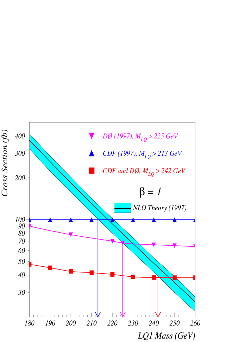
Figure 3: 95% CL upper cross section limits from CDF (triangles), DØ (inverted triangles), and combined (squares) leptoquark analyses. The band shows the NLO theoretical cross section; arrows correspond to the respective 95% CL lower mass limits.

6 Acknowledgements

We would like to thank all the CDF and DØ  members involved in the leptoquark searches. We thank the staffs at Fermilab and collaborating institutions for their contributions to this work, and acknowledge support from the Department of Energy and National Science Foundation (U.S.A.), the Italian Istituto Nazionale di Fisica Nucleare; the Ministry of Science, Culture, and Education of Japan; the Natural Sciences and Engineering Research Council of Canada; the National Science Council of the Republic of China; Commissariat à L’Energie Atomique (France), State Committee for Science and Technology and Ministry for Atomic Energy (Russia), CAPES and CNPq (Brazil), Departments of Atomic Energy and Science and Education (India), Colciencias (Colombia), CONACyT (Mexico), Ministry of Education and KOSEF (Korea), CONICET and UBACyT (Argentina), and the A. P. Sloan Foundation.

References

- [1] DØ Collaboration, B. Abbott et al., Phys. Rev. Lett. 79, 4321 (1997).
- [2] CDF Collaboration, F. Abe et al., Phys. Rev. Lett. 79, 4327 (1997).
- [3] H1 Collaboration, C. Adloff et al., Z. Phys. C 74, 191 (1997).
- [4] ZEUS Collaboration, J. Breitweg et al., Z. Phys. C 74, 207 (1997).
- [5] CDF Collaboration, F. Abe et al., Phys. Rev. D 50, 5518 (1994); ibid. D 50, 5535 (1994).
- [6] E710 Collaboration, R. Rubenstein et al., preprint Fermilab Conf–93/216-E (1993).
- [7] N.Amos et al., DØ Internal Note # 2186, unpublished (1994).
- [8] PDG Review of Particle Physics, Phys. Rev. D 54, 166 (1996).
- [9] M. Krämer, T. Plehn, M. Spira, and P.M. Zerwas, Phys. Rev. Lett. 79, 341 (1997).
- [10] R. Hollebeek, et al., Internal CDF Note 1109, unpublished (1990).