Correlations between $D$ and $\overline{D}$ mesons produced in 500 GeV/$c$ $\pi^{-}$-nucleon interactions

Abstract.

We present a study of correlations between $D$ and $\overline{D}$ mesons produced in 500 GeV/$c$ $\pi^{-}$-nucleon interactions, based on data from experiment E791 at Fermilab. We have fully reconstructed $791\pm 44$ charm meson pairs to study correlations between the transverse and longitudinal momenta of the two $D$ mesons and the relative production rates for different types of $D$ meson pairs. We see slight correlations between the longitudinal momenta of the $D$ and the $\bar{D}$, and significant correlations between the azimuthal angle of the $D$ and the $\bar{D}$. The experimental distributions are compared to a next-to-leading-order QCD calculation and to predictions of the Pythia/Jetset Monte Carlo event generator. We observe less correlation between transverse momenta and different correlations between longitudinal momenta than these models predict for the default values of the model parameters. Better agreement between data and theory might be achieved by tuning the model parameters or by adding higher order perturbative terms, thus contributing to a better understanding of charm production.

The relative production rates for the four sets of charm pairs, $D^{0}\overline{D}\!^{\;0}$, $D^{0}D^{-}$, $D^{+}\overline{D}\!^{\;0}$, $D^{+}D^{-}$, as calculated in the Pythia/Jetset event generator with the default parameters, agree with data as far as the relative ordering, but predict too many $D^{+}\overline{D}\!^{\;0}$ pairs and too few $D^{+}D^{-}$ pairs.

1 Introduction

Using data from experiment E791 at Fermilab, we reconstruct pairs of charm mesons produced in 500 GeV/$c$ $\pi^{-}$-nucleon interactions, where $\sqrt{s}=30.6$ GeV, and use correlations between the mesons to probe two aspects of the hadroproduction of mesons containing a heavy quark: the dynamics of the production of heavy quark-antiquark pairs and the subsequent hadronization of the quarks into hadrons. Correlations between the $D$ and $\overline{D}$ momenta transverse to the beam direction are sensitive to corrections to the leading-order calculations of the $c\overline{c}$ cross section. Correlations between the longitudinal momenta, as well as differences in the production rates of the four types of $D\overline{D}$ pairs ($D^{0}\overline{D}\!^{\;0}$, $D^{0}D^{-}$, $D^{+}\overline{D}\!^{\;0}$, and $D^{+}D^{-}$), provide information regarding the role of the remnants of the colliding hadrons in the hadronization process that transforms the charm quarks into charm mesons.

In most studies of the hadroproduction of charm particles, distributions for single charm particles are used to probe the underlying production physics [1, 2]. The variables used to describe the single particle distributions are the transverse momentum with respect to the beam direction, $p_{t}$, and either the rapidity $y$ or the Feynman scaling variable $x_{F}$, where

$$y\equiv\frac{1}{2}\ln\left(\frac{E+p_{z}}{E-p_{z}}\right){\rm and}$$ (1)

$$x_{F}\equiv p_{z}/{p_{z}^{max}}\approx 2p_{z}/\sqrt{s}.$$ (2)

$E$ and $p_{z}$ are the center-of-mass energy and longitudinal momentum of the charm particle and $\sqrt{s}$ is the total center-of-mass energy. The center of mass is that of the pion-nucleon system. Such single charm studies are insensitive to correlations between the two charm hadrons in a single event.

We have fully reconstructed $791\pm 44$ $D\overline{D}$ pairs. Based on this sample, we present background-subtracted, acceptance-corrected distributions for the following variables:

1. the invariant mass of the pair of charm mesons, $M_{D\overline{D}}$;

2. the square of the vector sum of the transverse momenta, with respect to the beam direction, of the $D$ and $\overline{D}$ mesons ($p^{2}_{t,D\overline{D}}\equiv|\mathchoice{\mbox{\boldmath$\displaystyle\bf p$}}{\mbox{\boldmath$\textstyle\bf p$}}{\mbox{\boldmath$\scriptstyle\bf p$}}{\mbox{\boldmath$\scriptscriptstyle\bf p$}}_{t,D}+\mathchoice{\mbox{\boldmath$\displaystyle\bf p$}}{\mbox{\boldmath$\textstyle\bf p$}}{\mbox{\boldmath$\scriptstyle\bf p$}}{\mbox{\boldmath$\scriptscriptstyle\bf p$}}_{t,\overline{D}}|^{2}$);

3. correlations between $x_{F,D}$ and $x_{F,\overline{D}}$, as well as $y_{D}$ and $y_{\overline{D}}$;

4. $\mathchar 257\relax x_{F}\equiv x_{F,D}-x_{F,\overline{D}}$ and $\mathchar 262\relax x_{F}\equiv x_{F,D}+x_{F,\overline{D}}$;

5. $\mathchar 257\relax y\equiv y_{D}-y_{\overline{D}}$ and $\mathchar 262\relax y\equiv y_{D}+y_{\overline{D}}$;

6. correlations between the squares of the magnitudes of the transverse momenta of the $D$ and $\overline{D}$ mesons, $p^{2}_{t,D}$ and $p^{2}_{t,\overline{D}}$;

7. $\mathchar 257\relax p_{t}^{2}\equiv|p^{2}_{t,D}-p^{2}_{t,\overline{D}}|$ and $\mathchar 262\relax p_{t}^{2}\equiv p^{2}_{t,D}+p^{2}_{t,\overline{D}}$;

8. the azimuthal separation between the momentum vectors of the $D$ and $\overline{D}$ mesons in the plane perpendicular to the beam direction, $\mathchar 257\relax\phi\equiv$ (minimum of $|\phi_{D}-\phi_{\overline{D}}|$ and $360^{\circ}-|\phi_{D}-\phi_{\overline{D}}|$);

9. correlations between the azimuthal separation ($\mathchar 257\relax\phi$) and the scalar sum and difference of the $D$ and $\overline{D}$ transverse momenta, $\mathchar 257\relax p_{t}^{2}$ and $\mathchar 262\relax p_{t}^{2}$ ;

In addition, this paper reports the relative production rates for each type of $D\overline{D}$ pair ($D^{0}\overline{D}\!^{\;0}$, $D^{0}D^{-}$, $D^{+}\overline{D}\!^{\;0}$, and $D^{+}D^{-}$), and compares the rapidity correlations for the various $D\overline{D}$ pair combinations.

We also investigate the extent to which the observed charm-pair correlations can be duplicated by simply convoluting the observed single charm particle distributions. In addition, we compare our measured distributions to three sets of theoretical predictions:

1. the distributions of $c\overline{c}$ pairs from a next-to-leading-order perturbative QCD calculation by Mangano, Nason and Ridolfi[3, 4];

2. the distributions of $c\overline{c}$ pairs from the Pythia/Jetset Monte Carlo event generator[5] which uses a parton-shower model to include higher-order perturbative effects[6]; and

3. the distributions of $D\overline{D}$ pairs from Pythia/Jetset which uses the Lund string model to transform $c\overline{c}$ pairs to $D\overline{D}$ pairs[7].

In Table 1, we compare the E791 charm-pair sample to those from other fixed-target experiments (both hadroproduction and photoproduction). The largest previous sample of fully-reconstructed hadroproduced charm pairs used to study correlations is 20 pairs from the CERN $\pi^{-}$-nucleon experiment NA32[10]. Some studies have been conducted with partially-reconstructed charm hadrons, in which the direction but not necessarily the magnitude of the charm particle momentum is determined directly. NA32 partially reconstructed 642 such charm pairs[11]. In photoproduction experiments, the largest sample of charm pairs reconstructed is from the E687 data[15], with 325 fully-reconstructed and 4534 partially-reconstructed charm pairs. In the E687 partially-reconstructed sample, one $D$ meson is fully reconstructed and the momentum vector of the other charm meson is determined by scaling the momentum vector of low-momentum charged pions from the decays $D^{*\pm}\rightarrow D^{0}\pi^{\pm}$.

Table 1.: Summary of fully-reconstructed and partially-reconstructed charm-pair samples from hadroproduction and photoproduction fixed-target experiments. In the last column, we list the physics variables studied in each experiment. The variables are defined in the text.

Experiment	Beam	Number	Measured Pair
	Energy(GeV),	of Pairs	Variables
	Beam Type,	Reconstructed
	and Target
E791	500 $\pi^{-}$	791 fully	$\mathchar 257\relax\phi$, $|\mathchar 262\relax\mathchoice{\mbox{\boldmath$\displaystyle\bf p$}}{\mbox{\boldmath$\textstyle\bf p$}}{\mbox{\boldmath$\scriptstyle\bf p$}}{\mbox{\boldmath$\scriptscriptstyle\bf p$}}_{t}|^{2}$, $\mathchar 262\relax p_{t}^{2}$,
			$\mathchar 257\relax p_{t}^{2}$, correlations,
(this paper)	Pt, C		$\mathchar 262\relax x_{F}$, $\mathchar 257\relax x_{F}$, $\mathchar 262\relax y$,
			$\mathchar 257\relax y$, $M_{D\overline{D}}$,
			$\sigma_{D^{0}\overline{D}^{0}}:\sigma_{D^{0}D^{-}}:$
			$\sigma_{D^{+}\overline{D}^{0}}:\sigma_{D^{+}D^{-}}$
WA92 [8]	350 $\pi^{-}$	475 partially	$\mathchar 257\relax\phi$, $|\mathchar 262\relax\mathchoice{\mbox{\boldmath$\displaystyle\bf p$}}{\mbox{\boldmath$\textstyle\bf p$}}{\mbox{\boldmath$\scriptstyle\bf p$}}{\mbox{\boldmath$\scriptscriptstyle\bf p$}}_{t}|^{2}$, $M_{D\overline{D}}$,
	Cu		$\mathchar 257\relax x_{F}$, $\mathchar 262\relax x_{F}$, $\mathchar 257\relax y$
E653 [9]	800 $p$	35 partially	$\mathchar 257\relax\phi$, $|\mathchar 262\relax\mathchoice{\mbox{\boldmath$\displaystyle\bf p$}}{\mbox{\boldmath$\textstyle\bf p$}}{\mbox{\boldmath$\scriptstyle\bf p$}}{\mbox{\boldmath$\scriptscriptstyle\bf p$}}_{t}|^{2}$,
	emulsion		$\mathchar 257\relax y$, $M_{D\overline{D}}$, $\cos\theta_{cm}$
NA32 [10][11]	230 $\pi^{-}$	20 fully	$|\mathchar 262\relax\mathchoice{\mbox{\boldmath$\displaystyle\bf p$}}{\mbox{\boldmath$\textstyle\bf p$}}{\mbox{\boldmath$\scriptstyle\bf p$}}{\mbox{\boldmath$\scriptscriptstyle\bf p$}}_{t}|^{2}$, $\mathchar 257\relax y$, $M_{D\overline{D}}$
(ACCMOR)	Cu	642 partially	$|\mathchar 262\relax\mathchoice{\mbox{\boldmath$\displaystyle\bf p$}}{\mbox{\boldmath$\textstyle\bf p$}}{\mbox{\boldmath$\scriptstyle\bf p$}}{\mbox{\boldmath$\scriptscriptstyle\bf p$}}_{t}|^{2}$, $\mathchar 257\relax y$, $M_{D\overline{D}}$, $\mathchar 257\relax\phi$
WA75 [12]	350 $\pi^{-}$	177 partially	$\mathchar 257\relax\phi$, $\mathchar 257\relax y$
	emulsion	120 partially	$M_{D\overline{D}}$, $\mathchar 262\relax x_{F}$, $\mathchar 262\relax p_{t}^{2}$
NA27 [13]	400 $p$	17 fully	$|\mathchar 262\relax\mathchoice{\mbox{\boldmath$\displaystyle\bf p$}}{\mbox{\boldmath$\textstyle\bf p$}}{\mbox{\boldmath$\scriptstyle\bf p$}}{\mbox{\boldmath$\scriptscriptstyle\bf p$}}_{t}|^{2}$, $\mathchar 262\relax x_{F}$, $\mathchar 257\relax y$, $M_{D\overline{D}}$
(LEBC)	H2	107 partially	$\mathchar 257\relax\phi$, $\sigma_{D^{0}\bar{D}^{0}}:$
			$\sigma_{D^{0}D^{-}+D^{+}\overline{D}^{0}}:\sigma_{D^{+}D^{-}}$
NA27 [14]	360 $\pi^{-}$	12 fully	$|\mathchar 262\relax\mathchoice{\mbox{\boldmath$\displaystyle\bf p$}}{\mbox{\boldmath$\textstyle\bf p$}}{\mbox{\boldmath$\scriptstyle\bf p$}}{\mbox{\boldmath$\scriptscriptstyle\bf p$}}_{t}|^{2}$, $\mathchar 262\relax x_{F}$,
			$\mathchar 257\relax y$, $M_{D\overline{D}}$
(LEBC)	H2	53 partially	$\mathchar 257\relax\phi$
E687 [15]	200 $\gamma$	$325$ fully	$\mathchar 257\relax\phi$, $|\mathchar 262\relax\mathchoice{\mbox{\boldmath$\displaystyle\bf p$}}{\mbox{\boldmath$\textstyle\bf p$}}{\mbox{\boldmath$\scriptstyle\bf p$}}{\mbox{\boldmath$\scriptscriptstyle\bf p$}}_{t}|^{2}$, $\mathchar 257\relax y$, $M_{D\overline{D}}$
	Be	4534 partially	$\mathchar 257\relax\phi$, $\mathchar 257\relax y$, $M_{D\overline{D}}$
NA14/2 [16]	100 $\gamma$	22 fully	$\mathchar 257\relax\phi$, $|\mathchar 262\relax\mathchoice{\mbox{\boldmath$\displaystyle\bf p$}}{\mbox{\boldmath$\textstyle\bf p$}}{\mbox{\boldmath$\scriptstyle\bf p$}}{\mbox{\boldmath$\scriptscriptstyle\bf p$}}_{t}|$, $\mathchar 262\relax p_{z}$,
	Si		$\mathchar 257\relax y$, $M_{D\overline{D}}$

In the analysis presented here, we have completed an extensive study of acceptance corrections. Acceptance corrections are made as a function of the eight variables that describe the $D$ and $\overline{D}$ degrees of freedom: $((y,p_{t},\phi,n)_{D},(y,p_{t},\phi,n)_{\overline{D}})$. Here $n$ is the number of decay tracks from the $D$ meson. Corrections are also made for the branching fractions of the reconstructed $D$ and $\overline{D}$ decay modes.

We performed a maximum likelihood fit to the two-dimensional reconstructed candidate $D$ mass distribution, including terms in the likelihood function for the true $D\overline{D}$ pairs that are the signal of interest, and also terms for combinations of a true $D$ with background, combinations of a true $\overline{D}$ with background, and combinations of two background candidates in the same event. From the full data set, the resulting number of true fully reconstructed $D\overline{D}$ pairs was $791\pm 44$. In making the distributions for single-charm and charm-pair physics variables, a likelihood fit was performed for each bin of the relevant physics variable.

Since we fully reconstruct both the $D$ and $\overline{D}$ meson, our results have fewer systematic errors than previously published results based on partially reconstructed pairs. In particular, we do not need to correct for missing tracks or possible contamination from baryons.

In the next section, we review the current theoretical understanding of the hadroproduction and hadronization of charm quarks. In the Appendix, we use both theoretical calculations and phenomenological models to investigate the dependence of various measurable properties of charm production on higher-order QCD effects, the charm quark mass, the parton distribution functions, the factorization scale and the renormalization scale. In Sec. 3, we describe the E791 detector and data processing. In Sec. 4, we describe the optimization of selection criteria for charm pairs. We discuss the extraction of background-subtracted distributions and corrections for acceptance effects in Sec. 5. In Sec. 6, we present the measured distributions for the charm pairs and compare them to the distributions predicted by (uncorrelated) single-charm distributions and to theoretical predictions. We summarize our results in Sec. 7.

2 Theoretical Overview

The charm quark is the lightest of the heavy quarks. Its relatively small mass ensures copious charm particle production at energies typical of fixed-target hadroproduction experiments. Its relatively large mass allows calculation of the large-momentum-transfer processes responsible for producing $c\overline{c}$ pairs using perturbative quantum chromodynamics (QCD). The consequence of the charm quark being the lightest heavy quark — more specifically, having a mass not sufficiently larger than $\mathchar 259\relax_{QCD}$ — is that there are considerable uncertainties associated with these calculations. Such large theoretical uncertainties, combined with conflicting experimental results from early charm hadroproduction experiments, have made systematic comparisons between theory and data difficult to interpret. Recent calculations of the full next-to-leading-order (NLO) differential cross sections by Mangano, Nason and Ridolfi (MNR)[3] and others, as well as unprecedented numbers of charm particles reconstructed by current fixed-target experiments, have allowed more progress to be made in this field.

In this section, we outline the theoretical framework used to describe the hadroproduction of charm pairs, focusing on the framework used by the following two packages: the FORTRAN program HVQMNR[4], which implements the MNR NLO perturbative QCD calculation for charm quarks, and the Pythia/Jetset Monte Carlo event generator[5], which makes predictions for charm particles based on leading order parton matrix elements, parton showers and the Lund string fragmentation model. In the Appendix we examine predictions from these two packages for the same beam type and energy as E791 for a wide range of theoretical assumptions to determine how sensitive the theoretical predictions are to

1. the inclusion of higher order terms ($\alpha_{s}^{3}$ or parton shower contributions); and

2. non-perturbative effects, including

   1. variations in parameters such as the mass of the charm quark and alternative parton distribution functions;

   2. changes in the factorization and renormalization scales; and

   3. other non-perturbative effects (hadronization and intrinsic transverse momentum of the colliding partons).

2.1 Charm Quark Production

Both the HVQMNR and Pythia/Jetset packages use a perturbative QCD framework to obtain the differential cross section for producing a $c\overline{c}$ pair:

$${\rm d}{\sigma_{c\overline{c}}}=\sum_{i,j}\int{\rm d}x_{b}\,{\rm d}x_{t}\,f_{i}^{b}(x_{b},\,\mu_{F})\,f_{j}^{t}(x_{t},\mu_{F})\,{\rm d}\hat{\sigma}_{ij}(x_{b}P_{b},x_{t}P_{t},p_{c},p_{\overline{c}},m_{c},\mu_{R}),$$ (3)

where

• $P_{b}$ ($P_{t}$) is the momentum of the beam (target) hadron in the center of mass of the colliding hadrons;

• $x_{b}$ ($x_{t}$) is the fraction of $P_{b}$ ($P_{t}$) carried by the hard-scattering parton from the beam (target) hadron;

• $f_{i}^{b}$ ($f_{i}^{t}$) is the parton distribution function for the beam (target) hadron;

• $\mu_{R}$, the renormalization scale, and $\mu_{F}$, the factorization scale, come from the perturbative QCD renormalization procedure which transforms the QCD coupling constant $g=\sqrt{4\pi\alpha_{s}}$ and the $\pi^{-}$ and nucleon wave functions from “bare” (infinite) values to physical (i.e., finite and measurable) values;

• ${\rm d}\hat{\sigma}_{ij}$ is the differential cross section for two hard-scattering partons to produce a pair of charm quarks, each with mass $m_{c}$, and with four-momenta $p_{c}$ and $p_{\overline{c}}$.

Leading order ($\alpha_{s}^{2}$) contributions to the $c\overline{c}$ cross section require the charm and anticharm quarks to be produced back-to-back in the center of mass of the $c\overline{c}$ pair. The (unknown) partonic center of mass is boosted in the beam direction with respect to the (known) hadronic center of mass. At fixed target energies, this boost smears the longitudinal momentum correlation while preserving the transverse correlation. Therefore, leading order calculations predict delta function distributions (i.e., maximal correlations) for variables which measure transverse correlations, such as $\mathchar 257\relax\phi_{c\overline{c}}=180^{\circ}$ and $p_{t,c\overline{c}}^{2}=0$, but predict small correlations in the longitudinal-momentum correlation variables $\mathchar 257\relax x_{F}$, $\mathchar 262\relax x_{F}$, $\mathchar 257\relax y$ and $\mathchar 262\relax y$.

These leading-order predictions are altered by the inclusion of higher order effects. The HVQMNR program adds the NLO ($\alpha_{s}^{3}$) corrections to the leading order calculation. NLO processes such as $gg\to c\overline{c}g$ produce $c\overline{c}$ pairs that are no longer back-to-back, smearing the leading order delta function distributions for $\mathchar 257\relax\phi_{c\overline{c}}$ and $p_{t,c\overline{c}}^{2}$.

The Pythia/Jetset event generator accounts for higher order perturbative QCD effects via a “parton shower” approach [17]. In this approach each of the two incoming and two outgoing partons, whose distributions are based on leading-order matrix elements, can branch — backwards and forwards in time respectively — into two partons, each of which can branch into two more partons, etc. This evolution continues until a small momentum scale is reached. In addition, the Pythia/Jetset event generator gives the hard-scattering partons an intrinsic transverse momentum $k_{t}$. Both the parton showers and the intrinsic transverse momentum tend to smear the transverse correlations, as shown in the Appendix.

The extent to which transverse-momentum correlations are smeared provides a measure of the importance of higher order perturbative effects. In addition, since the leading order calculation predicts very little longitudinal-momentum correlation, an enhancement of the longitudinal-momentum correlation also provides evidence for higher order perturbative effects or non-perturbative effects such as hadronization, described below.

2.2 Hadronization

The process whereby charm quarks are converted to hadrons is known as hadronization or fragmentation. Since this process occurs at an energy scale too low to be calculable by perturbative QCD, fragmentation functions are used to parameterize the hadronization of the charm quark. Such functions have been measured by several $e^{+}e^{-}$ experiments. The hadroproduction environment in $\pi^{-}$-N interactions, however, is quite different from the $e^{+}e^{-}$ environment. In $e^{+}e^{-}$ interactions, the light quarks in the produced charm hadrons must come from the vacuum. Hadroproduction leaves light quark beam and target remnants which are tied by the strong force to the charm quarks. Interactions between these remnants and the charm quarks can dramatically affect the momentum and flavor of the observed charm hadrons.

The Pythia/Jetset event generator uses the Lund string fragmentation framework, described in the Pythia/Jetset manual[5], to hadronize the charm quarks. To illustrate this model we consider an example from E791 where a gluon from a $\pi^{-}$ and a gluon from a nucleon in the target interact to form a $c\overline{c}$ pair. This accounts for $\sim 90\%$ of the theoretical cross section for 500 GeV/$c$ $\pi^{-}$-N interactions. After the gluon-gluon fusion, the remnant $\pi^{-}$ and nucleon are no longer color-singlet particles. The remnant $\pi^{-}$ is split into two valence quarks, and the remnant nucleon into a valence quark plus a diquark. Given this minimal set of partons — ($c$, $\overline{c}$), $(\overline{u},d)_{\pi}$, and $(qq,q)_{N}$ — the two dominant ways to make color-singlet strings, and the ones PYTHIA uses are[18]:

$$(c,\;\overline{u}_{\pi}), (\overline{c},\;q_{N}), {\rm and}\;\;(d_{\pi},\;qq_{N});\;{\rm or}$$ (4)

$$(\overline{c},\;d_{\pi}), (c,\;qq_{N}), {\rm and}\;\;(\overline{u}_{\pi},\;q_{N}).$$

In the center of mass of a particular $q\overline{q}$ system, such as $\overline{c}d$, the $\overline{c}$ and $d$ are moving apart along the string axis. As they move apart, energy is transferred to the color field. When this energy is great enough, $q\overline{q}$ pairs are created from the vacuum with equal and opposite transverse momentum (with respect to the string axis) according to a Gaussian distribution. The transverse momentum relative to the string axis of the resulting $\overline{c}q$ meson is determined by the $q$ quark since the $\overline{c}$ contributes none. The longitudinal momentum of the meson is given by a fragmentation function which describes the probability that a meson will carry off a fraction $z$ of the available longitudinal momentum. By default, heavy quark fragmentation is performed according to a Lund fragmentation function [7] modified by Bowler [19]:

$$f(z)\;\propto\;\frac{(1-z)^{a}}{z^{1+bm_{Q}^{2}}}\exp\left(\frac{-bm_{t}^{2}}{z}\right)$$ (5)

where $m_{t}^{2}\equiv M_{h}^{2}+\,p_{t}^{2}$ is the transverse mass of the hadron and $m_{Q}$ is the mass of the heavy quark. The default Pythia/Jetset settings are $a=0.3$ and $b=0.58\;({\rm GeV}/c^{2})^{-2}$.

When the remaining energy in the string drops below a certain cutoff (dependent on the mass of the remaining quarks) a coalescence procedure is followed, which collapses the last partons into a hadron while conserving energy. The entire string system is then boosted back into the lab frame. In the case of a $(\overline{c},\,d_{\pi})$ or $(c,\,\overline{u}_{\pi})$ string, this boost will tend to increase the longitudinal momentum of the charm hadron with respect to the charm quark since the $d_{\pi}$ and $\overline{u}_{\pi}$ will tend to have large longitudinal momentum. The opposite will occur, however, for a $(\overline{c},\,q_{N})$ string.

In some fraction of events, strings will be formed with too little energy to generate $q\overline{q}$ pairs from the vacuum. In these cases the $c$ quark (antiquark) will coalesce into a single meson with the beam antiquark (quark) or will coalesce into a single baryon (meson) with the target diquark (“bachelor” quark). This will tend to enhance production of charm hadrons with a light quark in common with a valence beam quark in the forward direction (beam fragmentation region) and production of charm hadrons with a light valence quark or diquark in common with the target in the target fragmentation region. This phenomenon has been used to explain the leading particle effect seen in charm hadroproduction experiments[20]–[25].

However, in most events, the string has sufficient energy to produce at least one $q\overline{q}$ pair from the vacuum. In this type of beam/target “dragging,” the strength of the dragging is not dependent on the light quark content of the produced particle.

These effects are evident in Fig. 1, which shows a scatter plot of the charm and anticharm rapidities for Pythia/Jetset $D\overline{D}$ events. Comparison of the scatter plot of the charm and anticharm quark rapidities, Fig. 1a, to the scatter plot of the $D$ and $\overline{D}$ rapidities, Fig. 1b, clearly demonstrates that significant correlations are introduced by hadronization.

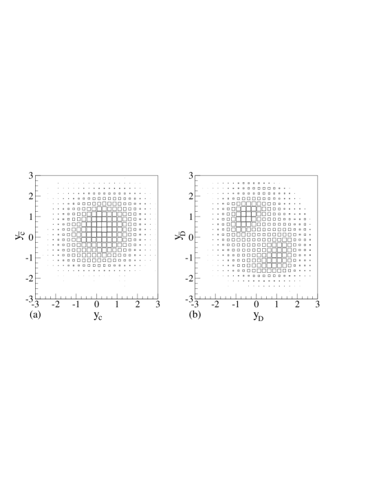
Fig. 1.: Scatter plots of $y_{\overline{c}}$ vs. $y_{c}$ and $y_{\overline{D}}$ vs. $y_{D}$, from 100,000 Pythia/Jetset $c\overline{c}$ and $D\overline{D}$ events, showing the correlation introduced by the hadronization model. As discussed in Sec. 4, we only reconstruct $D\overline{D}$ events in the region $-0.5<y_{D,\overline{D}}<2.5$.

Both the degree of correlation between the $D$ and $\overline{D}$ longitudinal momenta as well as differences in production of the four types of $D\overline{D}$ pairs — $D^{0}\overline{D}\!^{\;0}$, $D^{0}D^{-}$, $D^{+}\overline{D}\!^{\;0}$ and $D^{+}D^{-}$ — provide information about the charm quark hadronization process in a hadronic environment.

3 Experiment E791

The results reported in this paper are based on a data sample recorded by Fermilab experiment E791 during the 1991/92 fixed-target run. The E791 spectrometer is illustrated in Fig. 2. A 500 GeV/$c$ $\pi^{-}$ beam impinged on platinum and carbon targets. The spectrometer consisted of proportional wire chambers (PWC’s) and silicon microstrip detectors (SMD’s) upstream and downstream of the targets, two magnets, 35 drift chamber (DC) planes, two Čerenkov counters, an electromagnetic calorimeter, a hadronic calorimeter and a muon detector composed of an iron shield and two planes of scintillation counters.

Fig. 2.: The E791 spectrometer.

The spectrometer was an upgraded version of the apparatus used in Fermilab experiments E516, E691, and E769[26]. The major differences between the earlier versions and E791 were the addition of more planes of SMD’s, enhancement of the muon identification system, new front-end detector-signal digitizers and a new data acquisition system. In general, E791 finds that the most important parts of the spectrometer for analysis are the charged-particle tracking system and the threshold Čerenkov counters; although the threshold Čerenkov counters were used minimally in the analysis reported in this paper.

3.1 Target

The target consisted of five foils with center-to-center separations that varied from 14.8 to 15.4 mm. The most upstream foil was 0.5 mm thick and was made of platinum to provide a significant interaction probability in a thin target. The next four foils were 1.6 mm thick and were made of industrial diamond. The low Z of these carbon targets minimized multiple scattering, while the higher density of diamond permitted thinner downstream targets for the same interaction probability. The total pion interaction length of all five targets was about 1.9%. This target arrangement was chosen so that most of the particles with lifetimes and momenta within the range of interest to this experiment have a decay vertex in the gaps, where there is less background from secondary interactions.

3.2 The Spectrometer

The $\pi^{-}$ beam particle was tracked with eight PWC planes and six SMD planes upstream of the target region. Downstream of the targets, the charged-particle tracking system consisted of 17 SMD planes, two PWC planes, and 35 drift chamber planes. In general several planes of tracking chambers with different angular orientations around the beam axis were grouped together in each tracking station to provide hit ambiguity resolution. The various coordinates ($x$, $y$, $w$, $u$, $v$) measured by the planes in the tracking chamber stations were defined relative to a right-handed coordinate system $x-y-z$ in which increasing $z$ was in the beam direction, $x$ was the horizontal dimension and $y$ increases vertically upward. The $w$, $u$ and $v$ axes were rotated by $+60^{\circ}$, $+20.5^{\circ}$, and $-20.5^{\circ}$ with respect to the positive $x$ axis.

The beam PWC’s[27] had a wire spacing of 1 mm and were arranged in two stations widely separated in $z$ to measure the angle of the incoming beam particle with high precision. The first station was 31 m upstream, and the second was 12 m upstream of the last carbon target. Each station consisted of 4 planes: two staggered $x$ planes, a $y$ plane and a $w$ plane.

The beam SMD’s had a pitch of 25 $\mu$m and were also arranged in two stations, each with an $x$, $y$ and $w$ plane. The first SMD station was 80 cm upstream of the most downstream target, and the second station was 30 cm upstream of this target. The system of SMD’s downstream of the targets started 2.8 cm downstream of the last target and extended for 45 cm. It had a maximum angular acceptance of about $\pm$125 mr in both $x$ and $y$. Each of the first two planes ($x$ and $y$) had an active area of 2.5 cm by 5 cm, a pitch of 25 $\mu$m in the central 9.6 mm and 50 $\mu$m in the outer regions, and an efficiency of about 84%. The next nine planes were identical to those used in E691[28]. Each plane had a pitch of 50 $\mu$m, and an efficiency from 88% to 98%. They were instrumented to give an acceptance of  $\pm 100$ mrad with respect to the center of the most downstream target. They measured $x-y-v-y-x-v-x-y-v$ coordinates respectively. The final six SMD planes had active areas of 9 cm by 9 cm. The inner 3 cm had a pitch of 50 $\mu$m while the outer regions had an effective pitch of 200 $\mu$m. These measured $v-x-y-x-y-v$ coordinates. The efficiencies ranged from 96% to 99%.

The drift chambers were arranged in four stations as illustrated in Fig. 2. Each station was subdivided into substations with plane orientations such that an $x-y-z$ space point could be reconstructed in each substation. The characteristics of these chambers are given in Table 2. Since the beam, which operated at about 2 MHz throughout the run, passed through the center of the drift chambers in a small region instrumented with very few wires, each plane had a central inefficient region in which the efficiency decreased to $<10$% and the resolution was degraded by as much as a factor of four. The profile of the efficiency and resolution degradation region was approximately gaussian in an angular region of three to four mrad centered on the beam. The extent of the inefficient region increased with time during the run and is the major source of systematic uncertainty associated with the acceptance at large $x_{F}$. Each substation of the first drift chamber station was augmented by a PWC which measured the $y$ coordinate. These PWC’s had a wire spacing of 2 mm. Typical inclusive single charm acceptances for two, three, and four particle $D$ decays are shown in Fig. 3.

Table 2.: Characteristics of the DC tracking chambers for E791. “View” refers to the coordinate measured by that plane, with $u$ = $+20.5^{\circ}$, $v$ = $-20.5^{\circ}$ and $x^{\prime}$ staggered by one-half a wire spacing relative to the $x$ plane. The efficiency is for the region outside the central inefficient area.

Station	D1	D2	D3	D4
Approximate size (cm)	130 $\times$ 75	280 $\times$ 140	320 $\times$ 140	500 $\times$ 250
Number of substations	2	4	4	1
Views per substation	$x,\ x^{\prime},\ u,\ v$	$u,\ x,\ v$	$u,\ x,\ v$	$u,\ x,\ v$
$u$ and $v$ cell size (cm)	0.446	0.892	1.487	2.974
$x$ cell size (cm)	0.476	0.953	1.588	3.175
$z$ position of first plane	142.4	381.4	928.1	1738.
$z$ position of last plane	183.7	500.8	1047.1	1749.2
Approx. resolution ($\mu$m)	430	320	260	500
Typical efficiency	92%	93%	93%	85%

Fig. 3.: E791 acceptance functions vs. $x_{F}$ and $p_{t}^{2}$ for $K\pi$, $K\pi\pi$ and $K\pi\pi\pi$ candidates. The inclusive charm acceptance shown here was used to obtain approximately 150,000 reconstructed $D^{0}$ and $D^{+}$ charm meson decays in the E791 spectrometer as described, for example, in the study of single-charm production [29] and [30]. The $p_{t}^{2}$ acceptance is obtained for charm mesons with $-0.1<x_{F}<0.6$. The acceptance for events in which both charm particles are detected is quite different and is documented in detail later in this paper. (See Section 5.2.)

Momentum analysis was provided by two dipole magnets that bent particles in the same direction in the horizontal plane. The transverse momentum kicks were 212 MeV/$c$ for the first magnet and 320 MeV/$c$ for the second magnet. The centers of the two magnets were 2.8 m and 6.2 m downstream of the last target, respectively. The $x-y-z$ aperture of the pole faces of the first magnet was 183 cm by 81 cm by 100 cm and that of the second magnet was 183 cm by 86 cm by 100 cm.

Two segmented, gas-filled, threshold Čerenkov counters[31] provided particle identification over a large range of momenta. The threshold momenta above which a charged particle emits light were 6, 20 and 38 GeV/$c$ for $\pi$’s, $K$’s, and $p$’s, respectively, for the first counter, and 11, 36, and 69 GeV/$c$ for the second. The particle identification algorithm correlates the Čerenkov light observed in a given mirror-phototube segment with the charged particle tracking information. The algorithm indicates the likelihood that a charged particle of a given mass could have generated the observed Čerenkov light in the segment(s) in question.

The electromagnetic calorimeter, which we called the Segmented Liquid Ionization Calorimeter (SLIC), consisted of 20 radiation lengths of lead and liquid scintillator and was 19 m from the target. Layers of scintillator counters 3.17 and 6.24 cm wide were arranged transverse to the beam and their orientations alternated among horizontal and $\pm 20.5^{\circ}$ with respect to the vertical direction[32]. The hadronic calorimeter consisted of six interaction lengths of steel and acrylic scintillator. There were 36 layers, each with a 2.5-cm-thick steel plate followed by a plane of 14.3-cm-wide by 1-cm-thick scintillator slats; the slats were arranged alternately in the horizontal and vertical directions, and the upstream and downstream halves of the calorimeter were summed separately[33]. The signals from the hadronic calorimeter as well as those from the electromagnetic calorimeter were used for electron identification. Signals from both calorimeters were used to form the transverse energy requirement in the hardware trigger [34]. Electron identification was not used in this analysis.

Muons were identified by two planes of scintillation counters located behind a total of 15 interaction lengths of shielding, including the calorimeters. The first plane, 22.4 m from the target, consisted of twelve 40-cm-wide by 300-cm-long vertical scintillation counters in the outer region and three counters 60 cm wide in the central region. The second plane, added for E791, consisted of 16 scintillation counters 24.2 m from the target. These counters were each 14 cm wide and 300 cm long, and measured position in the vertical plane. These counters were equipped with TDC’s which provided information on the horizontal position of the incident muons [34]. Muon identification was not used in this analysis.

3.3 Trigger and Data Acquisition

To minimize biasing the charm data sample, the trigger requirements were very loose. The most significant requirements were that the signal in a scintillation counter downstream of the target be at least four times the most likely signal from one minimum-ionizing particle, and that the sum of the energy deposited in the electromagnetic and hadronic calorimeters, weighted by the sine of the angle relative to the beam, be above a threshold corresponding to 3 GeV of transverse energy. The time for the full hardware trigger decision was about 470 ns. This trigger was fully 100% efficient for charm decays.

A total of 24,000 channels were digitized and read out in 50 $\mu$s with a parallel-architecture data acquisition system[35]. Events were accepted at a rate of 9 kHz during the 23-second Tevatron beam spill. The typical recorded event size was 2.5 kbytes. Data were written continuously (during both the 23-second spill and the 34-second interspill periods) to forty-two Exabyte[36] model 8200 8-mm-tape drives at a rate of 9.6 Mbytes/s. Over $2\times 10^{10}$ hadronic interactions were recorded on 24,000 tapes.

3.4 Data Processing

The $2\times 10^{10}$ interactions recorded constitute about 50 Terabytes of data. Event reconstruction and filtering took place over a period of two and a half years at four locations: the University of Mississippi, The Ohio State University (moved to Kansas State University in 1993), Fermi National Accelerator Laboratory, and O Centro Brasileiro de Pesquisas Físicas, Rio de Janeiro (CBPF). The first three sites used clusters of commercial UNIX/RISC workstations controlled from a single processor with multiprocessor management software[37], while CBPF used ACP-II custom-built single-board computers[38].

As part of the reconstruction stage, a filter was applied which kept $\sim$20% of the events. This filter was effectively an offline trigger. To pass this filter, an event was required to have a reconstructed primary production vertex whose location coincided with one of the target foils. The event also had to include at least one of the following:

1. At least one reconstructed secondary decay vertex of net charge 0 for an even number of decay tracks and $\pm 1$ for an odd number of decay tracks. The longitudinal separation of the secondary vertex from the primary had to be at least four sigma for secondary vertices with three or more tracks and at least six sigma for vertices with two tracks, where sigma is the error in the separation,

2. At least one reconstructed $K_{s}\rightarrow\pi^{-}\pi^{+}$ or $\mathchar 259\relax\rightarrow p\pi$ candidate whose decay was observed upstream of the first magnet,

3. and for part of the run, at least one reconstructed $\phi\rightarrow K^{+}K^{-}$ candidate.

For one-third of the data sample, several other classes of events were also kept. These are included in analyses not covered in this paper:

1. Events in which the net charge of all the reconstructed tracks was negative and their total momentum was a large fraction of the beam momentum.

2. $K_{s}\rightarrow\pi^{-}\pi^{+}$ or $\mathchar 259\relax\rightarrow p\pi$ candidates that decayed inside the aperture of the first magnet.

Following the initial reconstruction/filter, which was applied to all events, additional selections of events were made to further divide the large data sample into subsets by class of physics analysis.

3.5 Detector Performance

The important detector performance characteristics for this analysis are the resolution for reconstructing the positions of both the primary interaction and secondary decay vertices, the efficiency for reconstructing the trajectories of charged particles, the resolution for measuring charged track momenta, and the efficiency and the misidentification rates for identifying charged pions and kaons using information from the Čerenkov counters.

The resolution for measuring the position of the primary vertex along the beam direction varies from about 240 $\mu$m for the most downstream target foil to 450 $\mu$m for the upstream foil. The variation is due to the extrapolation from the SMD system and to multiple scattering in material downstream of the interaction. The mean number of reconstructed tracks used to fit the primary vertex is seven. The measured secondary vertex resolution depends on the decay mode, the momentum of the $D$, and the selection criteria. For example, the vertex resolutions along the beam direction for $K^{-}\pi^{+}$ and $K^{-}\pi^{+}\pi^{-}\pi^{+}$ are 320 and 395 $\mu$m, respectively, for a mean $D^{0}$ momentum of 65 GeV/$c$, and worsen by 33 and 36 $\mu$m for every 10 GeV/$c$ increase in $D^{0}$ momentum.

The total efficiency, including acceptance, for reconstructing charged tracks is approximately 80% for particles with a momentum greater than 30 GeV/$c$ and drops to around 60% for particles of momentum 10 GeV/$c$. (This includes the inefficiency in the beam region.) For tracks which pass through both magnets and have a momentum greater than 10 GeV/$c$, the average resolution for measuring charged particle momentum $p$ is $\delta p/p=0.6\%\oplus(0.02p)\%$ where $\oplus$ stands for the quadratic sum, and $p$ is in GeV/$c$. Tracks which pass through only the first magnet have a resolution $\delta p/p=2\%\oplus(0.1p)\%$. The mean $D$ mass resolution for hadronic decays to two, three and four charged particles varies from 13 to 8 MeV/$c^{2}$ as the decay multiplicity increases. The mass resolution varies by about a factor of 2 between low and high momentum $D$ mesons.

In most E791 analyses, the Čerenkov counters play a very important role [39]. However, in this analysis with the two fully reconstructed D-meson decays, the Čerenkov counters play a minimal role. We use the Čerenkov counters for charged kaon identification. The kaon identification efficiencies and misidentification probabilities vary with longitudinal and transverse momentum and with the signatures required in the Čerenkov counters. For typical particle momenta in the range 20 GeV/$c$ to 40 GeV/$c$, and for the nonstringent criteria used for some of the final states, in this analysis, the Čerenkov identification efficiency for a kaon ranged from 64% to 72% while the probability for a pion to be misidentified as a kaon ranged from 6% to 12%.

A complete Monte Carlo simulation of the apparatus was used in this analysis to calculate the efficiency and investigate systematic effects. The simulation included all relevant physical processes such as multiple interactions and multiple scattering as well as geometrical apertures and resolution effects. It produced data in the same format as the real experiment. That Monte Carlo data was then reconstructed and analyzed with the same software as the real data.

4 Event Selection

In each E791 event, we search for two charm mesons ($D^{0}$, $\overline{D}\!^{\;0}$, $D^{+}$ or $D^{-}$) decaying to Cabibbo-favored final states that can be reconstructed with relatively high efficiency: $D^{0}\to K^{-}\pi^{+}$, $D^{0}\to K^{-}\pi^{+}\pi^{-}\pi^{+}$, $D^{+}\to K^{-}\pi^{+}\pi^{+}$, and the charge conjugate modes. To optimize the efficiency for reconstructing charm pairs, we search for both $D$ candidates simultaneously, rather than searching for the two candidates consecutively. In such a simultaneous search, we can require that one candidate or the other satisfy a fairly stringent selection criterion based on a particular variable used to discriminate charm decays from background, or that both candidates satisfy less stringent criteria.

We start with a sample of events, each containing two candidate $K^{-}\pi^{+}$, $K^{-}\pi^{+}\pi^{+}$ or $K^{-}\pi^{+}\pi^{-}\pi^{+}$ combinations with invariant mass between 1.7 and 2.0 GeV$/c^{2}$, and rapidity in the range $-0.5<y_{D,\overline{D}}<2.5$. These candidates are found by looping over all reconstructed tracks. The primary vertex is then refit after removing tracks which are associated with either candidate. No particle identification requirements are applied at this time. Candidates are rejected if any charged track, the primary vertex or either of the two secondary vertices do not meet minimal fit quality criteria. The sample of candidate pairs that pass just these criteria is dominated by combinatoric backgrounds. To choose further selection criteria, we use this sample to represent background. To represent signal, we use reconstructed charm pairs generated with the Monte Carlo program described at the end of the previous section. We then search for selection criteria that provide optimal discrimination between signal and background.

In order to extract the signal, we use selection criteria defined by discrimination variables (properties of the candidate event) and minimum or maximum allowed values for each variable. For candidate pairs with the same final states (i.e., both $K\pi$, both $K\pi\pi$, or both $K\pi\pi\pi$), the same discrimination variables and maximum or minimum values are used for both candidate $D$’s; for pairs with different final states, the discrimination variables are allowed to be different for the two candidate $D$’s.

The discrimination variables used address the following questions. Is a $D$ candidate consistent with originating from the primary interaction vertex? Is the vertex formed by the decay products of a $D$ candidate well separated from the primary interaction vertex and not inside a target foil? Do any of the decay products of the $D$ candidate appear to originate from the primary interaction vertex or from the other $D$ candidate vertex? Is the scalar sum of the squares of the transverse momenta of the $D$ candidate decay products, with respect to the $D$ candidate trajectory, indicative of a heavy meson decay? Is the Čerenkov information for the kaon candidate consistent with that for a real kaon? As an example of the cuts used: the $p_{t}$ balance cut was 400 MeV/$c$, and the secondary vertices were separated from the primary vertices by 8 times the rms-uncertainty in the separation.

To optimize the significance of the signal, we repeatedly choose the selection criterion that maximizes $N_{S}/\sqrt{N_{S}+N_{B}}$ while rejecting no more than 5% of the (Monte Carlo) signal. $N_{S}$ is the number of signal pairs satisfying the selection criterion, determined by Monte Carlo simulation, and $N_{B}$ is the number of background pairs, determined from the data. This requires properly normalizing the number of signal pairs in the Monte Carlo to the number of signal pairs in the data. When the background becomes dominated by pairs with only one true $D$ decay, we exclude from the background sample only those pairs in which both $D$ candidates lie in a narrow range around the $D$ mass.

We iterate the procedure of finding the optimal selection criterion (always allowing variables to be reused in subsequent iterations) until the significance of the signal no longer increases. The selection criteria are optimized separately for each of five decay topologies of $D\overline{D}$ pairs: 2-2, 3-3, 2-3, 2-4 and 3-4, where each integer represents the number of charged particles in the decay. We find that selection criteria are more often applied to one $D$ candidate or the other, rather than to both, especially early in the optimization procedure. In several cases, a criterion will be applied to one of the $D$ candidates, and a more stringent criterion involving the same discrimination variable will be applied to the other.

After optimizing our selection criteria, we end up with a sample of 9254 events in the data with both $D$ candidates in the mass range 1.7 to 2.0 GeV$/c^{2}$ and in the rapidity range $-0.5$ to $2.5$. Only pairs in which the two $D$ candidates have opposite charm quantum numbers are included in this sample. No significant signal for $DD$ or $\overline{D}\>\!\overline{D}$ pairs is observed. In Fig. 4, we plot the mass of the $D$ candidate versus the mass of the $\overline{D}$ candidate, for all five types of pairs. Three types of candidate pairs are evident in this scatter plot. Combinatoric background pairs consisting of a fake $D$ and a fake $\overline{D}$ candidate are spread over the entire plot. The density of these points decreases linearly with increasing candidate-$D$ mass. Pairs containing one real and one fake $D$ candidate appear as horizontal and vertical bands (called $D$ and $\overline{D}$ ridge events, respectively). In the center of the plot, we see an enhancement due to the crossing of the two bands and due to real pairs of $D$ mesons.

Fig. 4.: Scatter plot of the $D$-candidate mass versus the $\overline{D}$-candidate mass for the final unweighted charm-pair sample.

5 Data Analysis

In this section we describe the analysis procedures by which we determine the number of signal events in the full data sample shown in Fig. 4, as well as in each bin of the physics variables used to study the charm-pair production. Acceptance corrections include geometric acceptance, relative branching ratios, reconstruction efficiencies, and event selection efficiencies.

5.1 Determination of Yields

The experimental resolution for the $D$ mass measurement in the E791 spectrometer depends on both the $D$ decay mode and the $x_{F}$ of the $D$ meson, and the mean reconstructed mass depends on the decay mode. Therefore, we fit to the normalized $D$ mass defined as

$$M_{n}\equiv{M-M_{D}\over\sigma_{M}},$$ (6)

where $M$ is the measured mass, $M_{D}$ is the mean measured mass for the particular decay mode of the $D$ candidate, and $\sigma_{M}$ is the experimental resolution for the particular decay mode and $x_{F}$ of the $D$ candidate.

In this analysis we use the maximum likelihood method which assumes we have $N$ independent measurements of one or more quantities and that these quantities $\textstyle\bf z$ are distributed according to some probability density function $f(\mathchoice{\mbox{\boldmath$\displaystyle\bf z$}}{\mbox{\boldmath$\textstyle\bf z$}}{\mbox{\boldmath$\scriptstyle\bf z$}}{\mbox{\boldmath$\scriptscriptstyle\bf z$}};\mathchoice{\mbox{\boldmath$\displaystyle\bf\alpha$}}{\mbox{\boldmath$\textstyle\bf\alpha$}}{\mbox{\boldmath$\scriptstyle\bf\alpha$}}{\mbox{\boldmath$\scriptscriptstyle\bf\alpha$}})$ where $\textstyle\bf\alpha$ is a set of unknown parameters to be determined. To determine the set of values $\textstyle\bf\alpha$ that maximizes the joint probability for all events, we numerically solve the set of equations[40]:

$$\frac{\partial\ln L(\mathchoice{\mbox{\boldmath$\displaystyle\bf\alpha$}}{\mbox{\boldmath$\textstyle\bf\alpha$}}{\mbox{\boldmath$\scriptstyle\bf\alpha$}}{\mbox{\boldmath$\scriptscriptstyle\bf\alpha$}})}{\partial\alpha_{j}}=0\;\;{\rm where}\;\;L(\mathchoice{\mbox{\boldmath$\displaystyle\bf\alpha$}}{\mbox{\boldmath$\textstyle\bf\alpha$}}{\mbox{\boldmath$\scriptstyle\bf\alpha$}}{\mbox{\boldmath$\scriptscriptstyle\bf\alpha$}})=\prod_{i=1}^{N}f(\mathchoice{\mbox{\boldmath$\displaystyle\bf z$}}{\mbox{\boldmath$\textstyle\bf z$}}{\mbox{\boldmath$\scriptstyle\bf z$}}{\mbox{\boldmath$\scriptscriptstyle\bf z$}}_{i};\mathchoice{\mbox{\boldmath$\displaystyle\bf\alpha$}}{\mbox{\boldmath$\textstyle\bf\alpha$}}{\mbox{\boldmath$\scriptstyle\bf\alpha$}}{\mbox{\boldmath$\scriptscriptstyle\bf\alpha$}}).$$

The quantities that we measure for each event are the normalized mass of both the $D$ and $\overline{D}$ candidate; i.e., $\mathchoice{\mbox{\boldmath$\displaystyle\bf z$}}{\mbox{\boldmath$\textstyle\bf z$}}{\mbox{\boldmath$\scriptstyle\bf z$}}{\mbox{\boldmath$\scriptscriptstyle\bf z$}}=(M_{n}^{K^{-}m_{1}\pi}$, $M_{n}^{K^{+}m_{2}\pi}$). The unknown parameters in the maximum likelihood fit are the number of signal events, $N_{S}$; combinatoric events, $N_{C}$; events with one real $D$ and one combinatoric background called $D$-ridge events, $N_{D}$; events with one real $\overline{D}$ and one combinatoric background called $\overline{D}$-ridge events, $N_{\overline{D}}$; the slope of the background $K^{-}m_{1}\pi$ distribution, $S^{D}$; and the slope of the background $K^{+}m_{2}\pi$ distribution, $S^{\overline{D}}$. That is, the unknown parameters are

$$\mathchoice{\mbox{\boldmath$\displaystyle\bf\alpha$}}{\mbox{\boldmath$\textstyle\bf\alpha$}}{\mbox{\boldmath$\scriptstyle\bf\alpha$}}{\mbox{\boldmath$\scriptscriptstyle\bf\alpha$}}=(N_{S},N_{C},N_{D},N_{\overline{D}},S^{D},S^{\overline{D}}).$$

The terms $K^{-}m_{1}\pi$ and $K^{+}m_{2}\pi$ refer to $D$ or $\overline{D}$ decays into a kaon and $m_{i}$ pions.

We construct our probability density function using the following two assumptions: (i) the normalized mass distribution for background $K^{-}m_{1}\pi$ and $K^{+}m_{2}\pi$ is linear in $M_{n}^{K^{-}m_{1}\pi}$ and $M_{n}^{K^{+}m_{2}\pi}$, and (ii) the normalized mass distribution of real $D$’s and real $\overline{D}$’s is Gaussian with mean of 0 and sigma of 1. Under these assumptions, which are correct for our data, the probability density functions — normalized to unity in the two-dimensional window defined by $|M_{n}^{(K^{-}m_{1}\pi)}|<6.5$ and $|M_{n}^{(K^{+}m_{2}\pi)}|<6.5$ — for each class of events is

Combinatoric background:	$P_{C}=1/169+S^{D}M_{n}^{K^{-}m_{1}\pi}+S^{\overline{D}}M_{n}^{K^{+}m_{2}\pi},$
$D$-Ridge background events:	$P_{D}=(\frac{1}{13\sqrt{2\pi}}+\frac{N_{C}}{N_{D}}S^{\overline{D}}M_{n}^{K^{+}m_{2}\pi})\;e^{-(M_{n}^{K^{-}m_{1}\pi})^{2}/2},$
$\overline{D}$-Ridge background events:	$P_{\overline{D}}=(\frac{1}{13\sqrt{2\pi}}+\frac{N_{C}}{N_{\overline{D}}}S^{D}M_{n}^{K^{-}m_{1}\pi})\;e^{-(M_{n}^{K^{+}m_{2}\pi})^{2}/2},$
Signal events:	$P_{S}=\frac{1}{2\pi}e^{-((M_{n}^{K^{-}m_{1}\pi})^{2}+(M_{n}^{K^{+}m_{2}\pi})^{2})/2}.$

The distribution for each set of events is $N_{i}P_{i}$. The overall probability density function is then

$$f(\mathchoice{\mbox{\boldmath$\displaystyle\bf z$}}{\mbox{\boldmath$\textstyle\bf z$}}{\mbox{\boldmath$\scriptstyle\bf z$}}{\mbox{\boldmath$\scriptscriptstyle\bf z$}};\mathchoice{\mbox{\boldmath$\displaystyle\bf\alpha$}}{\mbox{\boldmath$\textstyle\bf\alpha$}}{\mbox{\boldmath$\scriptstyle\bf\alpha$}}{\mbox{\boldmath$\scriptscriptstyle\bf\alpha$}})=\frac{N_{C}P_{C}+N_{D}P_{D}+N_{\overline{D}}P_{\overline{D}}+N_{S}P_{S}}{N_{C}+N_{D}+N_{\overline{D}}+N_{S}}.$$

In this analysis, we use the extended maximum likelihood method[41, pg. 249] in which the number of $D\overline{D}$ candidates found, $N_{D\overline{D}}$, is considered to be one more measurement with a Gaussian probability distribution $G(N_{D\overline{D}},\mu)$ of mean $\mu=N_{C}+N_{D}+N_{\overline{D}}+N_{S}$ and $\sigma=\sqrt{\mu}$. Our likelihood function is then

$$L=G(N_{D\overline{D}},\mu)\;\prod_{i=1}^{N_{D\overline{D}}}f(\mathchoice{\mbox{\boldmath$\displaystyle\bf z$}}{\mbox{\boldmath$\textstyle\bf z$}}{\mbox{\boldmath$\scriptstyle\bf z$}}{\mbox{\boldmath$\scriptscriptstyle\bf z$}}_{i};\mathchoice{\mbox{\boldmath$\displaystyle\bf\alpha$}}{\mbox{\boldmath$\textstyle\bf\alpha$}}{\mbox{\boldmath$\scriptstyle\bf\alpha$}}{\mbox{\boldmath$\scriptscriptstyle\bf\alpha$}}).$$ (7)

To maximize the likelihood, we use the function minimization and error analysis FORTRAN package MINUIT [40]. Figure 5 shows the function
$N_{D\overline{D}}f(\mathchoice{\mbox{\boldmath$\displaystyle\bf z$}}{\mbox{\boldmath$\textstyle\bf z$}}{\mbox{\boldmath$\scriptstyle\bf z$}}{\mbox{\boldmath$\scriptscriptstyle\bf z$}};\mathchoice{\mbox{\boldmath$\displaystyle\bf\alpha$}}{\mbox{\boldmath$\textstyle\bf\alpha$}}{\mbox{\boldmath$\scriptstyle\bf\alpha$}}{\mbox{\boldmath$\scriptscriptstyle\bf\alpha$}})$ that maximizes the likelihood function for the final sample of $D\overline{D}$ candidates from Fig. 4 with $|M_{n}|\leq 6.5$, the mass range used for all fits in this analysis. The projections of the fit onto the $D$ and $\overline{D}$ axes are compared to the data in Fig. 6. The projected background contains both ridge events (one real $D$ and one combinatoric background) and events with two combinatoric background candidates. Therefore, the background under the charm-pair signal in the projected distribution is a linear distribution plus a Gaussian distribution, shown as the dotted line in the figure. The net charm-pair signal is shown as the residual after background subtraction.

Fig. 5.: The function that maximizes the joint probability of the unweighted charm-pair candidates from Fig. 4 with $|M_{n}|\leq 6.5$. The axes are the normalized candidate-$D$ masses $M_{n}$ defined in Eq. 6 in the text.

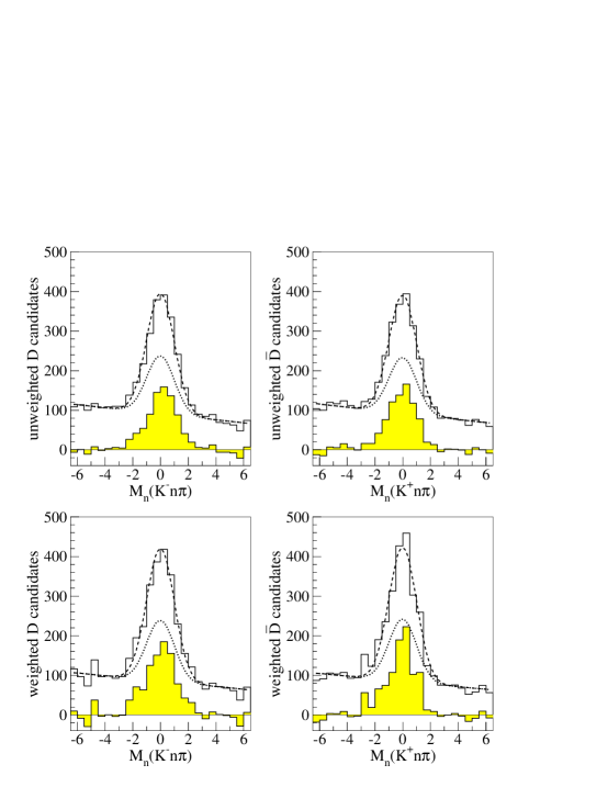
Fig. 6.: One-dimensional projections of the charm-pair normalized mass distributions for $D$ and $\overline{D}$ candidates, for unweighted events (top), and weighted events (bottom). The dashed curves are the fit projections. The dotted curves are the fit projections for the non-signal part of the fit. This includes background from one real $D$ ($\overline{D}$) and one fake $\overline{D}$ ($D$). The shaded histograms are the background-subtracted signals.

5.2 Acceptance Corrections

We determine the size of acceptance and smearing effects with a sample of approximately 7000 Monte Carlo simulated pairs that pass the same selection criteria as the real data. The size of the resolution with which we measure each charm-pair physics variable is much smaller than the range over which we bin that variable. Therefore, we ignore smearing effects.

We incorporate acceptance effects in the likelihood function for the fit by replacing the probability $p_{i}$ for event $i$ by $(p_{i})^{w_{i}}$ where $w_{i}$ is the weight for event $i$ [42]. The weight $w_{i}$ is inversely proportional to the efficiency and is normalized such that $\mathchar 262\relax_{i=1}^{N_{D\overline{D}}}w_{i}=N_{D\overline{D}}$, where $N_{D\overline{D}}$ is the number of $D\overline{D}$ candidates in the final sample. Corrections for relative branching fractions are also included in $w_{i}$, as described below. By construction, the mean of the weights is equal to 1. The standard deviation of the weights is 1.3. The total number of $D\overline{D}$ events found in the unweighted fit is $N_{s}=791\pm 44$. For the weighted likelihood fit, we find $N_{s}=910\pm 45$.

The efficiency depends not only on the detector acceptance but also on the relative branching fractions for the detected decay modes. By correcting for branching fractions, the final efficiency-corrected distributions reflect the relative production rates of the four types of $D\overline{D}$ pairs ($D^{0}\overline{D}\!^{\;0}$, $D^{0}D^{-}$, $D^{+}\overline{D}\!^{\;0}$, and $D^{+}D^{-}$) rather than the relative detected rates. We use the values $B(D^{+}\to K^{-}\pi^{+}\pi^{+})=(9.1\pm 0.6)\%$, $B(D^{0}\to K^{-}\pi^{+}\pi^{-}\pi^{+})=(8.1\pm 0.5)\%$, and $B(D^{0}\to K^{-}\pi^{+})=(4.01\pm 0.14)\%$[43].

A minimal independent set of properties that the acceptance could depend on is the decay mode of each of the $D$ mesons ($K^{-}\pi^{+}$, $K^{-}\pi^{+}\pi^{+}$, or $K^{-}\pi^{+}\pi^{-}\pi^{+}$), the rapidity $y$, the transverse momentum $p_{t}$, and the azimuthal angle $\phi$ of each of the $D$ mesons. In principle, we can use Monte Carlo simulated events to determine the acceptance for a particular candidate pair. The problem is the large number of Monte Carlo events that is needed to span such a large space (a 48-dimensional space, six variables for each pair of decay modes used). However, the efficiency function can be factorized for each combination of the $D$ decay modes, greatly increasing the statistical power of the Monte Carlo.

Using the Monte Carlo simulated events, we find that the acceptance of the $D$ is independent of the $\overline{D}$, and vice versa, at the level of the statistical precision of the simulation. This is true in spite of the correlations in the selection criteria described in Section 4. For each one, however, the shape of the acceptance as a function of $y$ depends on both the number of particles in the decay, $n_{D}$ or $n_{\overline{D}}$, and, at high $y$, whether the candidate decay is a $D$ or $\overline{D}$. The shape of the acceptance as a function of $p_{t}$ depends only on the number of particles in the decay, $n_{D}$ or $n_{\overline{D}}$. It is also found that the acceptance does not depend on the azimuthal angle $\phi$ of the $D$ or $\overline{D}$. Therefore, the acceptance function factorizes as follows:

$$A(n_{D},n_{\overline{D}},y_{D},y_{\overline{D}},p_{t,D},p_{t,{\overline{D}}},\phi_{D},\phi_{\overline{D}})$$

$$=b_{n_{D}}b_{n_{\overline{D}}}c(y_{D},y_{\overline{D}})d_{n_{D}}(p_{t,D})d_{n_{\overline{D}}}(p_{t,{\overline{D}}}),$$ (8)

where the subscripts, superscripts, and functional dependences of the terms b, c, and d are explicit, showing how the factorization is done.

We next determine which of the variables that describe the candidate pair, and for which the acceptance is not uniform, are correlated in the originally generated Monte Carlo. Such correlations could affect the apparent acceptance from the Monte Carlo if we simply integrate over a variable that is correlated with the variable for which we are determining the acceptance. We find that the most significant correlations in the Monte Carlo generator are between the variables $y_{D}$ and $y_{\overline{D}}$, where the acceptance is not uniform, and between the variables $\phi_{D}$ and $\phi_{\overline{D}}$, where the acceptance is uniform. Therefore, we cannot simply integrate over $y_{D}$ when determining the acceptance as a function of $y_{\overline{D}}$. Instead, we use the Monte Carlo to determine the two-dimensional acceptance function $c(y_{D},y_{\overline{D}})$ —which is independent of the Monte Carlo generated correlations — for each of the possible values of $n_{D}$ and $n_{\overline{D}}$ and use this function in Eq. 8. (This removes any dependence on the physics assumptions of the Monte Carlo from this equation.) Because of the uniform $\phi$ acceptance for the observed events, the double variable technique is not needed for $\phi$. Finally, the weight $w_{i}$ is calculated for each event such that it is proportional to ${1\over B(D)B(\overline{D})A}$ and $\mathchar 262\relax_{i=1}^{N_{D\overline{D}}}w_{i}=N_{D\overline{D}}$, where $N_{D\overline{D}}$ is the number of unweighted $D\overline{D}$ candidates in the final sample. Here $B$ is $B(D^{+}\to K^{-}\pi^{+}\pi^{+})$ for the charged $D$ candidates and $B$ is $B(D^{0}\to K^{-}\pi^{+}\pi^{-}\pi^{+})+B(D^{0}\to K^{-}\pi^{+})$ for the neutral $D$ candidates except for $D^{0}\overline{D}\!^{\;0}$ events where $B(D^{0})B(\overline{D}\!^{\;0})=B(D^{0}\to K^{-}\pi^{+})^{2}+2B(D^{0}\to K^{-}\pi^{+})B(D^{0}\to K^{-}\pi^{+}\pi^{-}\pi^{+})$ due to the exclusion of 4-4 pairs from the final sample.

5.3 Checks & Systematic Errors

Sources of systematic errors in our measurements include effects associated with the fitting procedure used to obtain the yields, the finite statistics of the Monte Carlo data sample used to generate the acceptance contributions to the weights, and imperfections in our modeling of the apparatus in the Monte Carlo.

For all the measured distributions, we compared the data to the two dimensional normalized mass distributions; in all cases, the fits qualitatively match the data. (For example, see Fig. 6.)

We also checked the fitting procedure by comparing the yields with those given by a simple counting method. In this method the normalized mass scatterplot was divided into regions corresponding to different combinations of signal, ridge, and combinatoric background events. The number of signal events was then found by subtracting the properly normalized number of events in the ridge and background regions from the central signal region. The results are in agreement, but the fitting technique gave smaller statistical errors, as expected.

The effect of the finite statistics in the Monte Carlo was determined by repeating the fits for the yields in each kinematic bin while varying the weight of each event randomly according to a Gaussian whose width corresponded to the statistical error on the weight. The systematic errors on the yields generated by this process were about $20\%$ of the statistical errors from the fit, which are negligible when added in quadrature.

As demonstrated in Figs. 7 to 12, in most cases the weighted and unweighted distributions are very similar. Statistical errors associated with modeling the acceptance are most important for events with large weights, but the number of events with large weights is small. We checked the effect of large weights by generating distributions without the large weight events, with no significant change. The distributions were also examined with all $K\pi\pi\pi$ candidates eliminated, the source of most of the events with a large acceptance correction. Again, the change did not significantly affect the distributions.

Fig. 7.: Single-charm distributions for $x_{F}$, $y$, $p_{t}^{2}$ and $\phi$, obtained from summing the $D$ and $\overline{D}$ distributions from our signal $D\overline{D}$ events; unweighted ($\circ$) and weighted ($\bullet$) data are described in Sec. 5.2.

Fig. 8.: Charm-pair distributions for $\mathchar 257\relax x_{F}=x_{F,D}-x_{F,\overline{D}}$ and $\mathchar 262\relax x_{F}=x_{F,D}+x_{F,\overline{D}}$. The uncorrelated single-charm predictions (——) for $\mathchar 257\relax x_{F}$ and $\mathchar 262\relax x_{F}$ are defined in Eqs. 9 and 10. Unweighted ($\circ$) and weighted ($\bullet$) data are described in Sec. 5.2.

Fig. 9.: Charm-pair distributions for $\mathchar 257\relax y=y_{D}-y_{\overline{D}}$ and $\mathchar 262\relax y=y_{D}+y_{\overline{D}}$. The uncorrelated single-charm predictions (——) for $\mathchar 257\relax y$ and $\mathchar 262\relax y$ are defined in Eqs. 9 and 10. Unweighted ($\circ$) and weighted ($\bullet$) data are described in Sec. 5.2.

Fig. 10.: Charm-pair distributions for $|\mathchar 257\relax p_{t}^{2}|=|p^{2}_{t,D}-p^{2}_{t,\overline{D}}|$ and $\mathchar 262\relax p_{t}^{2}=p^{2}_{t,D}+p^{2}_{t,\overline{D}}$. The uncorrelated single-charm predictions (——) for $\mathchar 257\relax p_{t}^{2}$ and $\mathchar 262\relax p_{t}^{2}$ are defined in Eqs. 9 and 10. Unweighted ($\circ$) and weighted ($\bullet$) data are described in Sec. 5.2.

Fig. 11.: Charm-pair distributions for $\mathchar 257\relax\phi=$ (minimum of $|\phi_{D}-\phi_{\overline{D}}|$ and $360^{\circ}-|\phi_{D}-\phi_{\overline{D}}|$) and $\mathchar 262\relax\phi=(\phi_{D}+\phi_{\overline{D}}$ modulo $360^{\circ})$. The uncorrelated single-charm predictions (——) for $\mathchar 257\relax\phi$ and $\mathchar 262\relax\phi$ are defined in Eqs. 9 and 10. Unweighted ($\circ$) and weighted ($\bullet$) data are described in Sec. 5.2.

Fig. 12.: Charm-pair distributions for $p^{2}_{t,D\overline{D}}=|\mathchoice{\mbox{\boldmath$\displaystyle\bf p$}}{\mbox{\boldmath$\textstyle\bf p$}}{\mbox{\boldmath$\scriptstyle\bf p$}}{\mbox{\boldmath$\scriptscriptstyle\bf p$}}_{t,D}~{}+\mathchoice{\mbox{\boldmath$\displaystyle\bf p$}}{\mbox{\boldmath$\textstyle\bf p$}}{\mbox{\boldmath$\scriptstyle\bf p$}}{\mbox{\boldmath$\scriptscriptstyle\bf p$}}_{t,\overline{D}}|^{2}$ and $M_{D\overline{D}}$. The solid histogram shows the uncorrelated single-charm predictions. The dashed $p^{2}_{t,D\overline{D}}$ histogram assumes that $x_{F,D}$ and $x_{F,\overline{D}}$ are uncorrelated and that $p^{2}_{t,D}$ and $p^{2}_{t,\overline{D}}$ are uncorrelated, but that $\phi_{D}$ and $\phi_{\overline{D}}$ are correlated as shown in Fig. 11. Unweighted ($\circ$) and weighted ($\bullet$) data are described in Sec. 5.2.

Another potential source of systematic error is uncertainty in the modeling of the beam-induced inefficiency in the centers of the drift chambers. The inefficiencies increased as the run progressed, primarily affecting $D$’s at large $x_{F}$. Since most $D$’s in the $D\overline{D}$ events are at low to modest $x_{F}$, the drift chamber inefficiencies did not have a significant effect on the relative efficiencies used in this analysis. We checked this by comparing the experimental results that had been efficiency-corrected with Monte Carlo simulations corresponding to different parts of the run, and found no significant differences.

In summary, systematic errors were found to be small relative to statistical errors.

6 Results

In this section, we present the background-subtracted, acceptance-corrected charm-pair distributions from the data and compare them to theoretical predictions. The Appendix contains an extensive discussion of the theoretical predictions for charm-pair distributions. As discussed in Sec. 4, all distributions — experimental and theoretical — are obtained after excluding any events in which the center-of-mass rapidity of either $D$ meson or either charm quark is less than $-0.5$ or greater than $2.5$.

For the experimental results, the acceptance-corrected distributions are obtained from maximizing the likelihood function with weighted events as discussed in Sec. 5.2. The uncorrected distributions are obtained from maximizing the unweighted likelihood function; the total number of signal $D\overline{D}$ events found in the unweighted fit is $N_{s}=791\pm 44$.

If the two charm mesons in each $D\overline{D}$ event are completely uncorrelated, then the charm-pair distributions contain no more information than the single-charm distributions. Before comparing the observed distributions to theoretical predictions, we use two methods to determine whether there exist correlations in the data. In the first method, described in Section 6.1, we convolute acceptance-corrected single-charm distributions to predict what the charm-pair distributions would be if the $D$ and $\overline{D}$ were uncorrelated. Comparing these single-charm predictions, the measured charm-pair distributions provide one measure of the degree of correlation between the $D$ and $\overline{D}$. In the second method, described in Section 6.2, we look directly for correlations by examining several two-dimensional distributions. For example, by finding the number of signal $D\overline{D}$ events per $y_{D}$ interval in several $y_{\overline{D}}$ intervals, we can determine whether the shape of the $y_{D}$ distribution depends on the value of $y_{\overline{D}}$. In Section 6.3, we compare our experimental distributions to the theoretical predictions discussed in Sec. 2 and in the Appendix. In Section 6.4, we examine integrated production asymmetries among the four types of $D\overline{D}$ pairs — $D^{0}\overline{D}\!^{\;0}$, $D^{0}D^{-}$, $D^{+}\overline{D}\!^{\;0}$, and $D^{+}D^{-}$ — and compare our experimental results to the predictions from the Pythia/Jetset event generator.

6.1 Single-Charm Predictions

In Fig. 7 we show the measured single-charm distributions for $x_{F}$, $y$, $p_{t}^{2}$ and $\phi$, as defined in Sec. 1. The single-charm distributions are obtained by fitting the two-dimensional normalized mass distributions for only those $D\overline{D}$ pairs in which the value of the single-charm variable for the candidate $D$ (or $\overline{D}$) is in the appropriate interval for each bin. In this way, the contribution to the single-charm signal from the $D$ and $\overline{D}$ ridge events is excluded. The distributions shown in Fig. 7 correspond to single-charm mesons from $D\overline{D}$ pairs in which the center-of-mass rapidity of both charm mesons lies between $-0.5$ and $+2.5$. Each distribution shown in Fig. 7 is obtained by summing the $D$ and $\overline{D}$ distributions. We have checked and found that the $D$ and $\overline{D}$ distributions are the same within statistical errors.

The vertical axis of each distribution gives the fraction of signal mesons per variable $v$ interval, $P(v)=\frac{1}{N_{D}}\frac{{\rm d}N_{D}}{{\rm d}v}$, where the total number of signal $D$ mesons $N_{D}$ is simply twice the number of signal $D\overline{D}$ events. Only a very small fraction (0% – 3%) of the signal events lie outside any of the ranges used in Figs. 7–11.

For each single-charm variable $v=x_{F}$, $y$, $p_{t}^{2}$, and $\phi$ we obtain two measured charm-pair distributions: the difference in $v$ for the two $D$’s, $\mathchar 257\relax v=v_{D}-v_{\overline{D}}$, and the sum of the $v$’s for the two $D$’s, $\mathchar 262\relax v=v_{D}+v_{\overline{D}}$. ($\mathchar 257\relax\phi$ is defined to be the minimum of $|\phi_{D}-\phi_{\overline{D}}|$ and $360^{\circ}-|\phi_{D}-\phi_{\overline{D}}|$, and $\mathchar 262\relax\phi$ is defined to be $\phi_{D}+\phi_{\overline{D}}$ modulo $360^{\circ}$.) In Figs. 8–11, we compare these measured charm-pair distributions to the charm-pair distributions one would generate from the measured single-charm distributions assuming the $D$ and $\overline{D}$ are completely uncorrelated, calculated as follows:

$$Q(\mathchar 257\relax v) = \int\int\delta(\mathchar 257\relax v-v_{D}+v_{\overline{D}})P(v_{D})P(v_{\overline{D}})dv_{D}dv_{\overline{D}}\,,$$ (9)

and

$$Q(\mathchar 262\relax v) = \int\int\delta(\mathchar 262\relax v-v_{D}-v_{\overline{D}})P(v_{D})P(v_{\overline{D}})dv_{D}dv_{\overline{D}}\,,$$ (10)

where $P(v)$ refers to the single-charm distributions shown in Fig. 7.

This convolution cannot be done with previously reported inclusive single charm distributions [25] since the inclusive distributions contain events which are excluded from the charm-pair sample, for example, events in which the $x_{F}$ of the unobserved $D$ is outside the acceptance or in which the unobserved charm particle is a charm baryon.

If the $D$ and $\overline{D}$ in the signal $D\overline{D}$ events are completely uncorrelated, then the measured charm-pair distributions for $\mathchar 257\relax v$ and $\mathchar 262\relax v$ should agree with the single-charm predictions, because both the charm-pair and single-charm distributions are for $D$ mesons with exactly the same restrictions on the rapidity of both $D$ mesons in the event. With the exception of the $\mathchar 257\relax\phi$ distribution (Fig. 11), the measured distributions are quite similar to the uncorrelated single-charm predictions, indicating both that the correlation between the $D$ and $\overline{D}$ longitudinal momenta is small and that the correlation between the amplitudes of the $D$ and $\overline{D}$ transverse momenta is small. The measured $\mathchar 257\relax x_{F}$ and $\mathchar 257\relax y$ distributions, however, are somewhat more peaked near zero than the single-charm predictions, possibly indicating slight longitudinal correlations.

Two other commonly used charm-pair variables are the square of the net transverse momentum of the charm pair, $p^{2}_{t,D\overline{D}}=|\mathchoice{\mbox{\boldmath$\displaystyle\bf p$}}{\mbox{\boldmath$\textstyle\bf p$}}{\mbox{\boldmath$\scriptstyle\bf p$}}{\mbox{\boldmath$\scriptscriptstyle\bf p$}}_{t,D}+\mathchoice{\mbox{\boldmath$\displaystyle\bf p$}}{\mbox{\boldmath$\textstyle\bf p$}}{\mbox{\boldmath$\scriptstyle\bf p$}}{\mbox{\boldmath$\scriptscriptstyle\bf p$}}_{t,\overline{D}}|^{2}$, and the invariant mass of the charm pair, $M_{D\overline{D}}$. The measured distributions and the uncorrelated single-charm predictions for these two variables are shown in Fig. 12. Obtaining these single-charm predictions for $p^{2}_{t,D\overline{D}}$ and $M_{D\overline{D}}$ is slightly more involved than for the $\mathchar 257\relax v$ and $\mathchar 262\relax v$ variables because $p^{2}_{t,D\overline{D}}$ and $M_{D\overline{D}}$ are not linear functions of $x_{F,D}$, $x_{F,\overline{D}}$, $\phi_{D}$, $\phi_{\overline{D}}$, $p^{2}_{t,D}$, and $p^{2}_{t,\overline{D}}$. Rather, in terms of these single-charm variables,

$$p^{2}_{t,D\overline{D}}=p^{2}_{t,D}+p^{2}_{t,\overline{D}}+2\sqrt{p^{2}_{t,D}p^{2}_{t,\overline{D}}}\cos(\phi_{D}-\phi_{\overline{D}}),\;{\rm and}$$

$$M_{D\overline{D}}=\sqrt{2M_{D}^{2}+2E_{D}E_{\overline{D}}-2\sqrt{p^{2}_{t,D}p^{2}_{t,\overline{D}}}\cos(\phi_{D}-\phi_{\overline{D}})-\frac{s\;x_{F,D}\;x_{F,\overline{D}}}{2}},$$

where the $D$ meson energy $E$ is $\sqrt{M_{D}^{2}+p^{2}_{t}+\frac{s\;x^{2}_{F}}{4}}$, and $s$ is the square of the center-of-mass energy of the colliding hadrons. We obtain single-charm predictions by randomly generating $10^{8}$ $D\overline{D}$ events in which all three variables ($x_{F}$, $\phi$, and $p_{t}^{2}$) for both $D$ mesons from each $D\overline{D}$ event are selected independently and randomly from a probability density function that is flat within the bins shown in Fig. 7, and zero elsewhere. Each event is weighted by

$$\frac{1}{|J|}P(x_{F,D})P(\phi_{D})P(p^{2}_{t,D})P(x_{F,\overline{D}})P(\phi_{\overline{D}})P(p^{2}_{t,\overline{D}}),$$

where $P(v)$ refers to the single-charm distributions shown in Fig. 7 and $|J|$ is the Jacobian determinant of the transformation from the complete and independent set of variables ($x_{F,D}$, $x_{F,\overline{D}}$, $\phi_{D}$, $\phi_{\overline{D}}$, $p^{2}_{t,D}$, and $p^{2}_{t,\overline{D}}$) to the set ($x_{F,D}$, $x_{F,\overline{D}}$, $\phi_{D}$, $\phi_{\overline{D}}$, $p^{2}_{t,D\overline{D}}$, and $M_{D\overline{D}}$). Specifically, $|J|=$

$$\left|\begin{array}[]{cc}1+\sqrt{\frac{p^{2}_{t,\overline{D}}}{p^{2}_{t,D}}}\cos(\phi_{D}-\phi_{\overline{D}})&1+\sqrt{\frac{p^{2}_{t,D}}{p^{2}_{t,\overline{D}}}}\cos(\phi_{D}-\phi_{\overline{D}})\\ \frac{1}{2\sqrt{2}M_{D\overline{D}}}\left(\frac{E_{\overline{D}}}{E_{D}}-\sqrt{\frac{p^{2}_{t,\overline{D}}}{p^{2}_{t,D}}}\cos(\phi_{D}-\phi_{\overline{D}})\right)&\frac{1}{2\sqrt{2}M_{D\overline{D}}}\left(\frac{E_{D}}{E_{\overline{D}}}-\sqrt{\frac{p^{2}_{t,D}}{p^{2}_{t,\overline{D}}}}\cos(\phi_{D}-\phi_{\overline{D}})\right)\end{array}\right|.$$

The measured distribution for $M_{D\overline{D}}$ agrees quite well with the uncorrelated single-charm prediction. The measured distribution for $p^{2}_{t,D\overline{D}}$, however, is steeper than the uncorrelated single-charm prediction, indicating the presence of correlations between $\mathchoice{\mbox{\boldmath$\displaystyle\bf p$}}{\mbox{\boldmath$\textstyle\bf p$}}{\mbox{\boldmath$\scriptstyle\bf p$}}{\mbox{\boldmath$\scriptscriptstyle\bf p$}}_{t,D}$ and $\mathchoice{\mbox{\boldmath$\displaystyle\bf p$}}{\mbox{\boldmath$\textstyle\bf p$}}{\mbox{\boldmath$\scriptstyle\bf p$}}{\mbox{\boldmath$\scriptscriptstyle\bf p$}}_{t,\overline{D}}$. The dashed histogram in Fig. 12 demonstrates that this lack of agreement is not due to the correlations between $\phi_{D}$ and $\phi_{\overline{D}}$ evident in the $\mathchar 257\relax\phi$ distribution in Fig. 11. This latter prediction is obtained by assuming that $x_{F,D}$ and $x_{F,\overline{D}}$ are uncorrelated and that $p^{2}_{t,D}$ and $p^{2}_{t,\overline{D}}$ are uncorrelated, but that $\phi_{D}$ and $\phi_{\overline{D}}$ are correlated as shown in Fig. 11. The correlations in $p^{2}_{t,D\overline{D}}$ should reflect similar correlations in $\mathchar 257\relax\phi$, $p^{2}_{t,D}$, and $p^{2}_{t,\overline{D}}$, since $p^{2}_{t,D\overline{D}}$ is a function of these variables. The fact that the disagreement in Fig. 12 is not so readily explained is a sign that the correlations can be subtle, and that there are additional correlations among the variables. In the following section we investigate correlations between $\mathchar 257\relax\phi$, $p_{t,D}$, and $p_{t,\overline{D}}$ in more detail.

6.2 Two-Dimensional Distributions

A direct method for investigating whether the variables $v_{D}$ and $v_{\overline{D}}$ are correlated is to determine the number of $D\overline{D}$ signal events per $v_{D}$ interval for a series of $v_{\overline{D}}$ intervals. Such two-dimensional distributions show whether the $v_{D}$ distribution depends on the value of $v_{\overline{D}}$, and vice-versa. Given the limited number of $D\overline{D}$ pairs, we use coarse binning to see statistically meaningful effects. In Figs. 13, 14 and 15, we show the results for $v=x_{F}$, $y$ and $p^{2}_{t}$, respectively. In part (a) of each figure, we show the number of acceptance-corrected $D\overline{D}$ signal events reconstructed in nine $(v_{D},\;v_{\overline{D}})$ bins — three $v_{D}$ bins times three $v_{\overline{D}}$ bins. Note that the three bin sizes are not equal. From the information in this two-dimensional plot, several normalized one-dimensional plots are created, facilitating our ability to detect differences in the shapes of the distributions. In particular, plot (b) in each figure shows the $v_{D}$ distribution for each $v_{\overline{D}}$ bin, $\frac{{\rm d}N_{s}}{{\rm d}v_{D}}/N_{i}$, where $N_{s}$ is the number of events in the relevant bin, and $N_{i}$ is the total number of events in the three $v_{D}$ bins. This normalization is chosen so that the integral over each $v_{D}$ distribution equals one. The symbols are defined in plot (a). Similarly, plot (c) in each figure shows the normalized $v_{\overline{D}}$ distribution for each $v_{D}$ bin. If the three sets of points in the figures (b) and (c) are statistically consistent, there are no significant correlations. Lastly, plots (d)–(f) simply rearrange the information shown in (b) and (c). Plot (d) shows the normalized $v_{D}$ and $v_{\overline{D}}$ distributions for the first $v_{\overline{D}}$ and $v_{D}$ bin, respectively; plot (e) shows results for the second bins; and plot (f) shows results for the third bins. In (d)-(f), agreement of the two sets of points implies that correlations in $v_{\overline{D}}$ are the same as correlations in $v_{D}$. The two-dimensional plots show the actual number of acceptance-corrected $D\overline{D}$ signal events in each bin, whereas the one-dimensional plots, proportional to $\frac{{\rm d}N_{s}}{{\rm d}v_{D}}$, take into account the variation in bin size.

Fig. 13.: (a) Number of weighted $D\overline{D}$ signal events d$N_{s}$ found in nine ($x_{F,D}$, $x_{F,\overline{D}}$) bins.  (b) $x_{F,D}$ distribution $({\rm d}N_{s}/{\rm d}x_{F,D})/N_{i}$ for each $x_{F,\overline{D}}$ bin, where $N_{i}$ is the total number of events in the three $x_{F,D}$ bins.  (c) $x_{F,\overline{D}}$ distribution for each $x_{F,D}$ bin.  (d)-(f) $x_{F,D}$ ($x_{F,\overline{D}}$) distribution for the first, second and third $x_{F,\overline{D}}$ ($x_{F,D}$) bins, respectively. Open symbols show the $x_{F,D}$ distributions; closed symbols show the $x_{F,\overline{D}}$ distributions. The weighting procedure is described in Sec. 5.2.

Fig. 14.: (a) Number of weighted $D\overline{D}$ signal events d$N_{s}$ found in nine ($y_{D}$, $y_{\overline{D}}$) bins. (b) $y_{D}$ distribution $({\rm d}N_{s}/{\rm d}y_{D})/N_{i}$ for each $y_{\overline{D}}$ bin, where $N_{i}$ is the total number of events in the three $y_{D}$ bins. (c) $y_{\overline{D}}$ distribution for each $y_{D}$ bin. (d)-(f) $y_{D}$ ($y_{\overline{D}}$) distribution for the first, second and third $y_{\overline{D}}$ ($y_{D}$) bins, respectively. Open symbols show the $y_{D}$ distributions; closed symbols show the $y_{\overline{D}}$ distributions. The weighting procedure is described in Sec. 5.2.

Fig. 15.: (a) Number of weighted $D\overline{D}$ signal events d$N_{s}$ found in nine ($p^{2}_{t,D}$, $p^{2}_{t,\overline{D}}$) bins. (b) $p^{2}_{t,D}$ distribution $({\rm d}N_{s}/{\rm d}p^{2}_{t,D}/N_{i})$ for each $p^{2}_{t,\overline{D}}$ bin, where $N_{i}$ is the total number of events in the three $p^{2}_{t,D}$ bins. (c) $p^{2}_{t,\overline{D}}$ distribution for each $p^{2}_{t,D}$ bin. (d)-(f) $p^{2}_{t,D}$ ($p^{2}_{t,\overline{D}}$) distribution for the first, second and third $p^{2}_{t,\overline{D}}$ ($p^{2}_{t,D}$) bins, respectively. Open symbols show the $p^{2}_{t,D}$ distributions; closed symbols show the $p^{2}_{t,\overline{D}}$ distributions. The weighting procedure is described in Sec. 5.2.

Figure 13 indicates some correlation between $x_{F,D}$ and $x_{F,\overline{D}}$. In particular, the first-bin distributions are more peaked at low $x_{F}$ than the second- and third-bin distributions of figures (b) and (c). This result is consistent with Fig. 8, discussed above, which shows that the measured $\mathchar 257\relax x_{F}$ distribution is somewhat steeper than the single-charm prediction. Because $x_{F}$ and $y$ are highly correlated, Fig. 14 shows the same trends as Fig. 13. Figure 15 indicates that $p^{2}_{t,D}$ and $p^{2}_{t,\overline{D}}$ are also slightly correlated — the second-bin $p^{2}_{t,D}$ and $p^{2}_{t,\overline{D}}$ distributions are enhanced in the second bin; and the third-bin $p^{2}_{t,D}$ and $p^{2}_{t,\overline{D}}$ distributions are enhanced in the third bin of figures (b) and (c). This result should be compared with Fig. 10, which is consistent with no correlation. Correlations are also seen in Fig. 12 which shows that the measured $p^{2}_{t,D\overline{D}}$ distribution is somewhat steeper than the uncorrelated single-charm prediction. In all three figures (13–15), the shapes of the three $v_{D}$ distributions are remarkably similar to the shapes of the respective $v_{\overline{D}}$ distributions as seen in figures (d)–(f). In Fig. 16 we investigate whether the separation in azimuthal angle between the $D$ and $\overline{D}$ is correlated to the amplitude of the transverse momenta of the $D$ and $\overline{D}$. In particular, we determine the number of signal $D\overline{D}$ events per $\mathchar 257\relax\phi$ interval in $\mathchar 262\relax p^{2}_{t}$ intervals and the number of signal $D\overline{D}$ events per $\mathchar 257\relax\phi$ interval in $|\mathchar 257\relax p_{t}^{2}|$ intervals. Although we find no significant correlation between $\mathchar 257\relax\phi$ and $|\mathchar 257\relax p_{t}^{2}|$, we find that $\mathchar 257\relax\phi$ and $\mathchar 262\relax p_{t}^{2}$ are quite correlated. The $\mathchar 257\relax\phi$ distribution is more peaked at large $\mathchar 262\relax p_{t}^{2}$ and the $\mathchar 262\relax p_{t}^{2}$ distribution is flatter at large $\mathchar 257\relax\phi$. A theoretical explanation for these correlations is discussed in the following section.

Fig. 16.: (a) Number of weighted $D\overline{D}$ signal events d$N_{s}$ found in nine ($\mathchar 257\relax\phi$, $\mathchar 262\relax p_{t}^{2}$) bins. (b) $\mathchar 257\relax\phi$ distribution $({\rm d}N_{s}/{\rm d}\mathchar 257\relax\phi)/N_{i}$ for each $\mathchar 262\relax p_{t}^{2}$ bin, where $N_{i}$ is the total number of events in the three $\mathchar 257\relax\phi$ bins. (c) $\mathchar 262\relax p_{t}^{2}$ distribution for each $\mathchar 257\relax\phi$ bin. (d) Number of weighted $D\overline{D}$ signal events d$N_{s}$ found in nine ($\mathchar 257\relax\phi$, $|\mathchar 257\relax p_{t}^{2}|$) bins. (e) $\mathchar 257\relax\phi$ distribution for each $|\mathchar 257\relax p_{t}^{2}|$ bin. (f) $|\mathchar 257\relax p_{t}^{2}|$ distribution for each $\mathchar 257\relax\phi$ bin. The weighting procedure is described in Sec. 5.2.

6.3 Comparisons with Theory

In this section, we compare all the acceptance-corrected distributions discussed in the previous two sections (Figs. 7–16) to three sets of theoretical predictions: the distributions of $c\overline{c}$ pairs from a next-to-leading-order (NLO) perturbative QCD calculation by Mangano, Nason and Ridolfi (MNR)[3, 4]; the distributions of $c\overline{c}$ pairs from the Pythia/Jetset Monte Carlo event generator[5] which uses a parton-shower model to include higher-order perturbative effects[6]; and the distributions of $D\overline{D}$ pairs from the Pythia (Version 5.7)/Jetset (Version 7.4) Monte Carlo event generator[5] which uses the Lund string model to transform $c\overline{c}$ pairs to $D\overline{D}$ pairs[7]. For all theoretical predictions, we use the default parameters suggested by the respective authors, which are discussed in the Appendix. All distributions are obtained after excluding any candidates in which the center-of-mass rapidity of either the $D$ or $\overline{D}$ (or, for the MNR calculation, the $c$ or $\overline{c}$) is less than $-0.5$ or greater than 2.5.

6.3.1 Single-Charm Distributions

Lack of agreement between an experimental charm-pair distribution and a theoretical prediction can arise if the theory does not model the correlations between the two charm particles correctly. However, it can also arise if the theory models the correlations correctly but does not correctly model the single-charm distributions. Hence, before comparing the experimental charm-pair distributions to theory, we first compare the acceptance-corrected single-charm distributions ($x_{F}$, $y$, $p_{t}^{2}$ and $\phi$) to theory in Fig. 17.

Fig. 17.: Single-charm distributions for $x_{F}$, $y$, $p_{t}^{2}$ and $\phi$: weighted data ($\bullet$) as described in Sec. 5.2; NLO QCD prediction (——); Pythia/Jetset charm quark prediction (${\scriptscriptstyle-\;\!-\;\!-\;\!-}$); and Pythia/Jetset $D$ meson prediction (${\scriptstyle\cdots\cdots\cdots}$). All distributions are obtained by summing the charm and anticharm distributions from charm-pair events.

For the longitudinal momentum distributions — $x_{F}$ and $y$ — the experimental results and theoretical predictions based on the default parameters do not agree. The experimental distributions are most similar to the NLO and Pythia/Jetset $c\overline{c}$ distributions, but are narrower than all three. The difference between the Pythia/Jetset $c\overline{c}$ and the Pythia/Jetset $D\overline{D}$ longitudinal distributions shows the effect of the hadronization scheme that color-attaches one charm quark to the remnant beam and the other to the remnant target, broadening the longitudinal distributions.

The experimental $p_{t}^{2}$ distribution agrees quite well with all three theoretical distributions. However, the Pythia/Jetset $c\overline{c}$ distribution is somewhat flatter; the Pythia/Jetset $D\overline{D}$ distribution is somewhat steeper. As expected, both the theoretical and experimental $\phi$ distributions are consistent with being flat.

6.3.2 Longitudinal Distributions for Pairs

The experimental and theoretical $\mathchar 257\relax x_{F}$ and $\mathchar 262\relax x_{F}$ distributions (Fig. 18) and $\mathchar 257\relax y$ and $\mathchar 262\relax y$ distributions (Fig. 19) do not agree with theoretical predictions derived from default parameters. This may be a reflection of the disagreement between the measured single-charm longitudinal distributions and theoretical models. As with the single-charm distributions, the experimental results are much closer to the two $c\overline{c}$ predictions than to the Pythia/Jetset $D\overline{D}$ prediction, but narrower than all three predictions. The Pythia/Jetset hadronization scheme introduces a strong correlation between the $D$ and $\overline{D}$ which significantly broadens the $\mathchar 257\relax y$ distribution. That is, hadronization tends to pull the $D\overline{D}$ apart, due to color string attachment to the incident hadronic remnants. As we show in Fig. 20, the Pythia/Jetset $D\overline{D}$ $\mathchar 257\relax y$ distribution is broader than the prediction we obtain by using the predicted single-charm distributions and assuming they are uncorrelated, as calculated using Eqn. 9. In contrast, the experimental $\mathchar 257\relax y$ distribution is slightly narrower than its uncorrelated single-charm prediction (Fig. 9).

Fig. 18.: Charm-pair $\mathchar 257\relax x_{F}$ and $\mathchar 262\relax x_{F}$ distributions; weighted data ($\bullet$) as described in Sec. 5.2; NLO QCD prediction (——); Pythia/Jetset charm quark prediction (${\scriptscriptstyle-\;\!-\;\!-\;\!-}$); and Pythia/Jetset $D$ meson prediction (${\scriptstyle\cdots\cdots\cdots}$).

Fig. 19.: Charm-pair $\mathchar 257\relax y$ and $\mathchar 262\relax y$ distributions; weighted data ($\bullet$) as described in Sec. 5.2; NLO QCD prediction (——); Pythia/Jetset charm quark prediction (${\scriptscriptstyle-\;\!-\;\!-\;\!-}$); and Pythia/Jetset $D$ meson prediction (${\scriptstyle\cdots\cdots\cdots}$).

Fig. 20.: Pythia/Jetset $D\overline{D}$ prediction for $\mathchar 257\relax y$ compared to the Pythia/Jetset single-charm prediction that is obtained by assuming that the $D$ and $\overline{D}$ mesons are completely uncorrelated (see Eq. 9).

6.3.3 Transverse Distributions for Pairs

In Figs. 21–23, we compare experimental distributions to theoretical predictions for the following transverse variables: $|\mathchar 257\relax p_{t}^{2}|$, $\mathchar 262\relax p_{t}^{2}$, $\mathchar 257\relax\phi$, $\mathchar 262\relax\phi$, and $p^{2}_{t,D\overline{D}}$. Any observed discrepancy between theory and data for the $|\mathchar 257\relax p^{2}_{t}|$, $\mathchar 257\relax\phi$, and $p^{2}_{t,D\overline{D}}$ distributions is noteworthy because the single-charm $p^{2}_{t}$ and $\phi$ experimental distributions agree well with theory. An observed discrepancy, therefore, must derive from the theory modeling the correlation between $\mathchoice{\mbox{\boldmath$\displaystyle\bf p$}}{\mbox{\boldmath$\textstyle\bf p$}}{\mbox{\boldmath$\scriptstyle\bf p$}}{\mbox{\boldmath$\scriptscriptstyle\bf p$}}_{t,D}$ and $\mathchoice{\mbox{\boldmath$\displaystyle\bf p$}}{\mbox{\boldmath$\textstyle\bf p$}}{\mbox{\boldmath$\scriptstyle\bf p$}}{\mbox{\boldmath$\scriptscriptstyle\bf p$}}_{t,\overline{D}}$ incorrectly.

If $\mathchoice{\mbox{\boldmath$\displaystyle\bf p$}}{\mbox{\boldmath$\textstyle\bf p$}}{\mbox{\boldmath$\scriptstyle\bf p$}}{\mbox{\boldmath$\scriptscriptstyle\bf p$}}_{t,D}$ and $\mathchoice{\mbox{\boldmath$\displaystyle\bf p$}}{\mbox{\boldmath$\textstyle\bf p$}}{\mbox{\boldmath$\scriptstyle\bf p$}}{\mbox{\boldmath$\scriptscriptstyle\bf p$}}_{t,\overline{D}}$ were completely uncorrelated, then the single-charm predictions (Figs. 10–12) would provide good estimates for these three distributions. At the opposite extreme, if $\mathchoice{\mbox{\boldmath$\displaystyle\bf p$}}{\mbox{\boldmath$\textstyle\bf p$}}{\mbox{\boldmath$\scriptstyle\bf p$}}{\mbox{\boldmath$\scriptscriptstyle\bf p$}}_{t,D}$ and $\mathchoice{\mbox{\boldmath$\displaystyle\bf p$}}{\mbox{\boldmath$\textstyle\bf p$}}{\mbox{\boldmath$\scriptstyle\bf p$}}{\mbox{\boldmath$\scriptscriptstyle\bf p$}}_{t,\overline{D}}$ were completely anticorrelated — as in the leading-order perturbative QCD prediction — then the $\mathchar 257\relax p^{2}_{t}$ distribution would be a delta function at $\mathchar 257\relax p^{2}_{t}=0\;{\rm GeV}^{2}$; the $p^{2}_{t,D\overline{D}}$ distribution a delta function at $p^{2}_{t,D\overline{D}}=0\;{\rm GeV}^{2}$; and the $\mathchar 257\relax\phi$ distribution a delta function at $\mathchar 257\relax\phi=180^{\circ}$. Both the experimental distributions and the three sets of theoretical predictions lie between these extremes. None of the three experimental distributions, however, is as steep as any of the theoretical predictions. The next-to-leading-order predictions are the steepest — that is, the next-to-leading-order calculation predicts the most correlation between $\mathchoice{\mbox{\boldmath$\displaystyle\bf p$}}{\mbox{\boldmath$\textstyle\bf p$}}{\mbox{\boldmath$\scriptstyle\bf p$}}{\mbox{\boldmath$\scriptscriptstyle\bf p$}}_{t,c}$ and $\mathchoice{\mbox{\boldmath$\displaystyle\bf p$}}{\mbox{\boldmath$\textstyle\bf p$}}{\mbox{\boldmath$\scriptstyle\bf p$}}{\mbox{\boldmath$\scriptscriptstyle\bf p$}}_{t,\overline{c}}$ as a model for $\mathchoice{\mbox{\boldmath$\displaystyle\bf p$}}{\mbox{\boldmath$\textstyle\bf p$}}{\mbox{\boldmath$\scriptstyle\bf p$}}{\mbox{\boldmath$\scriptscriptstyle\bf p$}}_{t,D}$ and $\mathchoice{\mbox{\boldmath$\displaystyle\bf p$}}{\mbox{\boldmath$\textstyle\bf p$}}{\mbox{\boldmath$\scriptstyle\bf p$}}{\mbox{\boldmath$\scriptscriptstyle\bf p$}}_{t,\overline{D}}$. Thus hadronization and higher-order perturbative effects smear out the $c\overline{c}$ correlations. The Pythia/Jetset hadronization scheme broadens the $\mathchar 257\relax\phi$ distribution, bringing it closer to the experimental results. The same hadronization scheme also narrows the $p^{2}_{t,D\overline{D}}$ and $\mathchar 257\relax p_{t}^{2}$ distributions, which makes them disagree even more with the experimental results. One mechanism which would broaden the $p^{2}_{t,D\overline{D}}$ and $\mathchar 257\relax p_{t}^{2}$ distributions as well as the $\mathchar 257\relax\phi$ distribution (bringing all into better agreement with the experimental results) is to increase the intrinsic transverse momentum of the colliding partons in the beam and target hadrons (see the Appendix, Secs. A.5 and A.6). An improved theoretical understanding may involve adding terms higher than NLO to calculations, although other authors find good agreement by choosing appropriate values for nonperturbative parameters [44].

Fig. 21.: Charm-pair $|\mathchar 257\relax p^{2}_{t}|$ and $\mathchar 262\relax p_{t}^{2}$ distributions; weighted data ($\bullet$) as described in Sec. 5.2; NLO QCD prediction (——); Pythia/Jetset charm quark prediction (${\scriptscriptstyle-\;\!-\;\!-\;\!-}$); and Pythia/Jetset $D$ meson prediction (${\scriptstyle\cdots\cdots\cdots}$).

Fig. 22.: Charm-pair $\mathchar 257\relax\phi$ and $\mathchar 262\relax\phi$ distributions; weighted data ($\bullet$) as described in Sec. 5.2; NLO QCD prediction (——); Pythia/Jetset charm quark prediction (${\scriptscriptstyle-\;\!-\;\!-\;\!-}$); and Pythia/Jetset $D$ meson prediction (${\scriptstyle\cdots\cdots\cdots}$).

Fig. 23.: Charm-pair $p^{2}_{t,D\overline{D}}$ and $M_{D\overline{D}}$ distributions: weighted data ($\bullet$) as described in Sec. 5.2; NLO QCD prediction (——); Pythia/Jetset charm quark prediction (${\scriptscriptstyle-\;\!-\;\!-\;\!-}$); and Pythia/Jetset $D$ meson prediction (${\scriptstyle\cdots\cdots\cdots}$).

6.3.4 Charm-Pair Invariant Mass

In Fig. 23, we compare the experimental charm-pair invariant mass distribution to the Pythia/Jetset prediction. The experimental $M_{D\overline{D}}$ distribution is steeper than the theoretical predictions. This is similar to the experimental single-charm $x_{F}$ (or $y$) distributions, which are also steeper than the theoretical predictions. (See Fig. 17.)

In addition, the correlations introduced by the Pythia/Jetset hadronization scheme broaden the invariant mass distribution.

6.3.5 Two-Dimensional Distributions

In Figs. 24–27, we examine the same two-dimensional experimental distributions discussed in Section 6.2. We now compare these experimental results to the three sets of theoretical predictions. In each figure, the top row shows the NLO perturbative QCD $c\overline{c}$ prediction; the middle row, the Pythia/Jetset $c\overline{c}$ prediction; and the bottom row, the Pythia/Jetset $D\overline{D}$ prediction. The experimental data points and errors are repeated in each row.

The longitudinal distributions, $x_{F}$ and $y$, are shown in Figs. 24 and 25. The three theoretical predictions are quite different. The NLO $c\overline{c}$ predictions show no significant correlation between $x_{F,D}$ and $x_{F,\overline{D}}$ (or between $y_{D}$ and $y_{\overline{D}}$) and the $x_{F,D}$ and $x_{F,\overline{D}}$ distributions are quite similar. The Pythia/Jetset $c\overline{c}$ predictions show a slight correlation and the $x_{F,D}$ and $x_{F,\overline{D}}$ distributions are somewhat different. Due to the Pythia/Jetset hadronization scheme, the Pythia/Jetset $D\overline{D}$ prediction shows the strongest correlation between $x_{F,D}$ and $x_{F,\overline{D}}$. Interestingly, in the Pythia/Jetset $D\overline{D}$ prediction, $x_{F,D}$ and $x_{F,\overline{D}}$ are anticorrelated; in the Pythia/Jetset $c\overline{c}$ prediction they are positively correlated. The correlation patterns in the experimental results, although inconsistent with any of the theoretical predictions, are closest to the Pythia/Jetset $c\overline{c}$ predictions.

Fig. 24.: (a) The NLO QCD prediction for the number of $c\overline{c}$ events in nine ($x_{F,D}$, $x_{F,\overline{D}}$) bins, normalized such that the number of NLO events equals the number of weighted $D\overline{D}$ signal events. (b) Experimental $x_{F,D}$ distribution for each $x_{F,\overline{D}}$ bin compared to the NLO QCD predictions. Each $x_{F,D}$ distribution is normalized such that the integral over $x_{F,D}$ equals one. (c) Same as (b) for the $x_{F,\overline{D}}$ distributions. (d)-(f) Same as (a)-(c) for the Pythia/Jetset $c\overline{c}$ prediction. (g)-(i) Same as (a)-(c) for the Pythia/Jetset $D\overline{D}$ prediction. Symbols represent weighted data; histograms represent theoretical predictions. $\triangle$ and —— correspond to the low bin; $\bullet$ and ${\scriptscriptstyle-\;\!-\;\!-\;\!-}$ to the middle bin; $\Box$ and ${\scriptstyle\cdots\cdots\cdots}$ to the high bin.

Fig. 25.: (a) The NLO QCD prediction for the number of $c\overline{c}$ events in nine ($y_{D}$, $y_{\overline{D}}$) bins, normalized such that the number of NLO events equals the number of weighted $D\overline{D}$ signal events. (b) Experimental $y_{D}$ distribution for each $y_{\overline{D}}$ bin compared to the NLO QCD predictions. Each $y_{D}$ distribution is normalized such that the integral over $y_{D}$ equals one. (c) Same as (b) for the $y_{\overline{D}}$ distributions. (d)-(f) Same as (a)-(c) for the Pythia/Jetset $c\overline{c}$ prediction. (g)-(i) Same as (a)-(c) for the Pythia/Jetset $D\overline{D}$ prediction. Symbols represent weighted data; histograms represent theoretical predictions. $\triangle$ and —— correspond to the low bin; $\bullet$ and ${\scriptscriptstyle-\;\!-\;\!-\;\!-}$ to the middle bin; $\Box$ and ${\scriptstyle\cdots\cdots\cdots}$ to the high bin.

In Fig. 26, we investigate the correlations between $p^{2}_{t,D}$ and $p^{2}_{t,\overline{D}}$. The three theoretical predictions and the experimental results all show similar trends. Although all the distributions are broader than the leading-order perturbative QCD prediction — a delta function at $p^{2}_{t,D}=p^{2}_{t,\overline{D}}$ — they all shows signs of an enhancement in the $p^{2}_{t,D}=p^{2}_{t,\overline{D}}$ bins. The Pythia/Jetset $c\overline{c}$ distributions and the Pythia/Jetset $D\overline{D}$ distributions are very similar and resemble the experimental results more so than the NLO $c\overline{c}$ distributions. All of the theoretical third-bin distributions are significantly flatter than the experimental third-bin distributions. In contrast to the longitudinal distributions, all the $p^{2}_{t,D}$ distributions are very similar to the respective $p^{2}_{t,\overline{D}}$ distributions.

Fig. 26.: (a) The NLO QCD prediction for the number of $c\overline{c}$ events in nine ($p^{2}_{t,D}$, $p^{2}_{t,\overline{D}}$) bins, normalized such that the number of NLO events equals the number of weighted $D\overline{D}$ signal events. (b) Experimental $p^{2}_{t,D}$ distribution for each $p^{2}_{t,\overline{D}}$ bin compared to the NLO QCD predictions. Each $p^{2}_{t,D}$ distribution is normalized such that the integral over $p^{2}_{t,D}$ equals one. (c) Same as (b) for the $p^{2}_{t,\overline{D}}$ distributions. (d)-(f) Same as (a)-(c) for the Pythia/Jetset $c\overline{c}$ prediction. (g)-(i) Same as (a)-(c) for the Pythia/Jetset $D\overline{D}$ prediction. Symbols represent weighted data; histograms represent theoretical predictions. $\triangle$ and —— correspond to the low bin; $\bullet$ and ${\scriptscriptstyle-\;\!-\;\!-\;\!-}$ to the middle bin; $\Box$ and ${\scriptstyle\cdots\cdots\cdots}$ to the high bin.

In Fig. 27, we investigate correlations between $\mathchar 257\relax\phi$ and $\mathchar 262\relax p_{t}^{2}$. For the $\mathchar 257\relax\phi$ dependence, a leading-order perturbative QCD calculation predicts a delta function at $\mathchar 257\relax\phi=180^{\circ}$. We expect perturbative predictions to be more accurate as the energy scale $Q$ of the partonic hard scattering increases:

$$Q\equiv\sqrt{m_{c}^{2}+\frac{p^{2}_{t,c}+p^{2}_{t,\overline{c}}}{2}}.$$ (11)

That is, we expect the $\mathchar 257\relax\phi$ distribution to be more peaked at $180^{\circ}$ for $D\overline{D}$ events with larger $\mathchar 262\relax p_{t}^{2}$. This behavior is clearly evident in our experimental distributions as well as in all three theoretical predictions. The theoretical $\mathchar 257\relax\phi$ distributions, however, for all three $\mathchar 262\relax p_{t}^{2}$ bins, are significantly steeper than the respective experimental distributions. The NLO $c\overline{c}$ $\mathchar 257\relax\phi$ distributions are the steepest. The experimental and theoretical $\mathchar 262\relax p_{t}^{2}$ distributions are in fairly good agreement, with the $\mathchar 262\relax p_{t}^{2}$ distribution broadening as $\mathchar 257\relax\phi$ increases. No significant correlation between $\mathchar 257\relax\phi$ and $|\mathchar 257\relax p_{t}^{2}|$ or between $\mathchar 257\relax\phi$ and $\mathchar 257\relax y$ is seen in the data or theory.

Fig. 27.: (a) The NLO QCD prediction for the number of $c\overline{c}$ events in nine ($\mathchar 257\relax\phi$, $\mathchar 262\relax p^{2}_{t}$) bins, normalized such that the number of NLO events equals the number of weighted $D\overline{D}$ signal events. (b) Experimental $\mathchar 257\relax\phi$ distribution for each $\mathchar 262\relax p^{2}_{t}$ bin compared to the NLO QCD predictions. Each $\mathchar 257\relax\phi$ distribution is normalized such that the integral over $\mathchar 257\relax\phi$ equals one. (c) Same as (b) for the $\mathchar 262\relax p^{2}_{t}$ distributions. (d)-(f) Same as (a)-(c) for the Pythia/Jetset $c\overline{c}$ prediction. (g)-(i) Same as (a)-(c) for the Pythia/Jetset $D\overline{D}$ prediction. Symbols represent weighted data; histograms represent theoretical predictions. $\triangle$ and —— correspond to the low bin; $\bullet$ and ${\scriptscriptstyle-\;\!-\;\!-\;\!-}$ to the middle bin; $\Box$ and ${\scriptstyle\cdots\cdots\cdots}$ to the high bin.

6.4 Dependence of Yields and Longitudinal Correlations on Type of $D\overline{D}$ Pair

6.4.1 Relative Yields

In Table 3, we compare the experimental yields for each type of $D\overline{D}$ pair to the predictions from the Pythia/Jetset event generator and to a naive spin-counting model. The experimental results are obtained by maximizing the weighted likelihood function where the weights account for both acceptance effects and the relative branching fractions of the reconstructed decay modes (Sec. 5.2). Again, for both data and Pythia/Jetset predictions, the results are for pairs in which the rapidities of both the $D$ and $\overline{D}$ lie between $-0.5$ and $2.5$. The Pythia/Jetset and naive spin-counting models both assume that vector $D^{*}$ production is three times more likely than pseudoscalar $D$ production due to the number of spin states and that contributions from higher spin states are negligible. They also use the known $D^{*\pm}$ branching fractions, $B(D^{*+}\to D^{0}\pi^{+})=68.3\%$ and $B(D^{*+}\to D^{+}X)=31.7\%$, to determine $D$ production. The differences between the Pythia/Jetset and naive spin-counting model come from the Pythia/Jetset hadronization scheme — in particular, the rate of coalescence. As discussed in Sec. 2.2, a charm quark tied to a valence quark by a low-mass string can coalesce with that valence quark into a meson. This will tend to increase the rate of $D^{-}(\overline{c}d)$ and $D^{0}(c\overline{u})$ production in the forward region for the E791 $\pi^{-}(\overline{u}d)$ beam. Since $D^{*-}$ decays to $\overline{D}\!^{\;0}$, production of $\overline{D}\!^{\;0}$ will also be enhanced. This effect is seen in Table 3 where the number of pairs that contain a $D^{+}$ is reduced while the number of pairs that contain a $D^{-},D^{0},$ or $\overline{D}\!^{\;0}$ is increased in the Pythia/Jetset model relative to the naive model. Both models agree with data as far as the relative ordering but predict too many $D^{0}\overline{D}\!^{\;0}$ pairs and too few $D^{+}D^{-}$ pairs.

Table 3.: Normalized acceptance-corrected experimental yields for the four types of $D\overline{D}$ pairs compared to predictions from a naive spin-counting model and the Pythia/Jetset event generator. Experimental and Pythia/Jetset yields are for $-0.5<y_{D,\overline{D}}<2.5$. Statistical and systematic errors are given for the data.

	Data	Spin-counting model	Pythia/Jetset
$D^{0}\overline{D}\!^{\;0}$	$0.50\pm 0.04\pm 0.01$	0.572	$0.604\pm 0.002$
$D^{0}D^{-}$	$0.20\pm 0.02\pm 0.01$	0.184	$0.208\pm 0.002$
$D^{+}\overline{D}\!^{\;0}$	$0.18\pm 0.02\pm 0.01$	0.184	$0.138\pm 0.002$
$D^{+}D^{-}$	$0.12\pm 0.02\pm 0.01$	0.060	$0.051\pm 0.001$

6.4.2 Correlations Between the $D$ and $\overline{D}$ Longitudinal Momenta

As shown in Fig. 28, in the Pythia/Jetset hadronization scheme, the correlation between $y_{D}$ and $y_{\overline{D}}$ is quite different for each of the four types of $D\overline{D}$ pairs. In Fig. 29, we investigate whether this is also true for data. Given the limited size of our data sample, we can only search for gross asymmetries in the ($y_{D}$, $y_{\overline{D}}$) distributions. We obtain the four plots in Fig. 29 by bisecting the two-dimensional ($y_{D}$, $y_{\overline{D}}$) distributions along the following four lines ($v=a$): $\mathchar 257\relax y=0$, $\mathchar 262\relax y=1.2$, $y_{D}=0.6$, and $y_{\overline{D}}=0.6$. These four lines are indicated by dashed lines in Fig. 28.

Fig. 28.: Pythia/Jetset prediction for the ($y_{D}$, $y_{\overline{D}}$) distribution for each of the four types of $D\overline{D}$ pairs. The dashed lines help define the asymmetry functions $A_{v}(i)$ (Eq. 12) shown in Fig. 29.

Fig. 29.: The asymmetry function $A_{v}(i)=\frac{N_{i}(v>a)-N_{i}(v<a)}{N_{i}(v>a)+N_{i}(v<a)}$, where $i=$($D^{0}\overline{D}\!^{\;0}$, $D^{0}D^{-}$, $D^{+}\overline{D}\!^{\;0}$, $D^{+}D^{-}$) and $N_{i}$ is the number of signal $D\overline{D}$ events of type $i$, for ($v$, $a$) = ($\mathchar 257\relax y$, $0$), ($\mathchar 262\relax y$, $1.2$), ($y_{D}$, $0.6$), and ($y_{\overline{D}}$, $0.6$). Both the weighted data (open symbols) and the Pythia/Jetset (closed symbols) distributions correspond to events in which $-0.5<y_{D},y_{\overline{D}}<2.5$.

To search for possible differences in asymmetries, we determine whether the fraction of signal events on one side of a given line depends on the type of $D\overline{D}$ pair. Specifically, for both theory and data, we show in Fig. 29

$$A_{v}(i)=\frac{N_{i}(v>a)-N_{i}(v<a)}{N_{i}(v>a)+N_{i}(v<a)}$$ (12)

where $i=(D^{0}\overline{D}\!^{\;0},D^{0}D^{-},D^{+}\overline{D}\!^{\;0},D^{+}D^{-})$ and $N_{i}$ is the number of signal $D\overline{D}$ events of type $i$. The Pythia/Jetset $A_{\mathchar 262\relax y}$ distribution is fairly flat, indicating no significant differences among the four $D\overline{D}$ types for the $\mathchar 262\relax y$ distribution. The Pythia/Jetset $A_{\mathchar 257\relax y}$, $A_{y_{D}}$, and $A_{y_{\overline{D}}}$ distributions, however, indicate significant differences, all of which are easily interpreted in terms of the Pythia/Jetset coalescence mechanism discussed in Sec. 2. Unfortunately, our experimental errors are of the same order as the degree of differences in the Pythia/Jetset predictions. The experimental $A_{y_{D}}$ distribution, for example, is consistent with the Pythia/Jetset prediction, but it is also consistent with being flat. Similarly, the experimental $A_{\mathchar 262\relax y}$ distribution is fairly consistent with the flat Pythia/Jetset prediction, but it also shows some indication of a difference between $D^{0}\overline{D}\!^{\;0}$ and $D^{+}D^{-}$. The most significant difference between the experimental results and the Pythia/Jetset predictions occurs for the $D\overline{D}$ types $D^{0}\overline{D}\!^{\;0}$ and $D^{+}D^{-}$ in the $A_{y_{\overline{D}}}$ distribution. Both theory and data indicate a difference between $D^{0}\overline{D}\!^{\;0}$ and $D^{+}D^{-}$; however, we find experimentally that $A_{y_{\overline{D}}}(D^{0}\overline{D}\!^{\;0})>A_{y_{\overline{D}}}(D^{+}D^{-})$, whereas the Pythia/Jetset model finds $A_{y_{\overline{D}}}(D^{+}D^{-})>A_{y_{\overline{D}}}(D^{0}\overline{D}\!^{\;0})$.

7 Conclusions

We fully reconstructed $791\pm 44$ true $D\overline{D}$ pairs after all background subtractions. This is the largest such sample of charm pairs used in an analysis of the hadroproduction of $c\overline{c}$ to date. The full reconstruction of the final states of both $D$ mesons offers several advantages over some of the previous studies that have used partially reconstructed $D$ candidates. We are able to correct the data for both detector inefficiencies and for the branching fractions of the observed decays so that the acceptance-corrected distributions represent the produced mixture of $D$ mesons, rather than the detected mixture. Because the final states are fully reconstructed, we are able to calculate both the magnitude and direction of the $D$ momenta. Therefore, we are able to thoroughly investigate the degree of correlation between both the transverse and longitudinal components of the momenta, with respect to the beam direction, of the $D$ and $\overline{D}$.

We have compared all the measured acceptance-corrected distributions to predictions of the fully differential next-to-leading-order calculation for $c\overline{c}$ production by Mangano, Nason and Ridolfi [3, 4], as well as to predictions from the Pythia/Jetset Monte Carlo event generator [5] for $c\overline{c}$ [6] and $D\overline{D}$ production [7].

7.1 Transverse Correlations

Our measurements indicate that the transverse momenta of the $D$ and $\overline{D}$ in charm-pair events are correlated in several ways. (See Secs. 6.2 and 6.3.5.) The square of the amplitudes of the $D$ and $\overline{D}$ transverse momenta are slightly correlated (Fig. 15). The directions of the $D$ and $\overline{D}$ in the plane transverse to the beam axis are significantly correlated (Fig. 11). The separation in azimuthal angle, $\mathchar 257\relax\phi$, is significantly correlated with the sum of the squares of the $D$ and $\overline{D}$ transverse momenta, $\mathchar 262\relax p^{2}_{t}$ (Fig. 16). These features have been observed by several other experiments [8, 9, 10, 11, 12, 13, 14, 15, 16]. Using the default parameters, the three models yield the same trend in correlations as we find in data. The models also predict that the relative transverse angles of the $D$ and $\overline{D}$ are more correlated than we find in data (Fig. 22). These results provide an opportunity to tune the default parameters, or add higher order terms in the models, to obtain better agreement with data [44].

7.2 Longitudinal Correlations

Our measurements indicate that the longitudinal momenta of the $D$ and $\overline{D}$ from charm-pair events are slightly correlated. The measured $\mathchar 257\relax x_{F}$ and $\mathchar 257\relax y$ distributions (Figs. 8–9) are somewhat narrower than what one would predict from the observed single-charm predictions assuming no correlations. The $x_{F,D}$ ($y_{D}$) distribution depends on the value of $x_{F,\overline{D}}$ ($y_{\overline{D}}$), and vice-versa (Figs. 13–14).

The single-charm $x_{F}$ and $y$ distributions from the three theoretical models do not agree with each other or with the measured distributions (Fig. 17). The three models predict different correlations between the charm and anticharm longitudinal momenta (Figs. 24–25) — the next-to-leading-order calculation predicts no significant correlation; the Pythia/Jetset $c\overline{c}$ prediction indicates a slight positive correlation; and the Pythia/Jetset $D\overline{D}$ prediction indicates a strong negative correlation. The $D\overline{D}$ data agree best with the Pythia/Jetset $c\overline{c}$ prediction. The disagreement between the models and the data might be corrected by adjusting the non-perturbative parameters in the models, or by adding higher order terms.

7.3 Dependence of Yields and Longitudinal Correlations on Type of $D\overline{D}$ Pair

The relative yields of the four types of charm pairs, $D^{0}\overline{D}\!^{\;0}$, $D^{0}D^{-}$, $D^{+}\overline{D}\!^{\;0}$, and $D^{+}D^{-}$, as calculated in the Pythia/Jetset event generator, agree with data as far as their ordering but disagree with regard to number of pairs produced, predicting too many $D^{0}\overline{D}\!^{\;0}$ pairs and too few $D^{+}D^{-}$ pairs. (See Table 3.) We studied the degree to which longitudinal correlations depend on the type of $D\overline{D}$ pair in data and in the Pythia/Jetset event generator. Although we see differences between data and the event generator (Fig. 29), the statistical uncertainties on the measured correlations are too large to make any conclusive statements.

7.4 Summary and Discussion

The charm-pair distributions presented in this paper provide an opportunity to extend our understanding of charm production beyond what was previously possible with single-charm and lower-statistics or partially reconstructed charm-pair distributions. The measured distributions and observed correlations can be compared to the predictions of models, testing assumptions in the models and providing discrimination among different values for the free parameters in the models. Some comparisons have been made in the paper and in the Appendix.

Before comparing the measurements to predictions, we looked for correlations directly in the charm-pair data by comparing the observed $D\overline{D}$ pair distributions with the convolution of the measured single-charm distributions assuming no correlations. We find that the charm-pair distributions are quite similar to the convoluted single-charm distributions, indicating little correlation between the two charm mesons in an event, with the exception of the distributions for $\mathchar 257\relax\phi$ and $p^{2}_{t,D\overline{D}}$. The $\mathchar 257\relax\phi$ distribution shows clear evidence of correlations, and the $p^{2}_{t,D\overline{D}}$ distribution is steeper than the uncorrelated single-charm prediction. In addition, the data are consistent with possible small correlations in the $\mathchar 257\relax x_{F}$ and $\mathchar 257\relax y$ pair distributions, which are somewhat more peaked near zero than the single-charm convolutions.

In the comparisons of the measured and predicted charm-pair distributions, we observe less correlation between transverse momenta and different correlations between longitudinal momenta than theoretical models predict, for the default values of parameters in the models. Work by other authors suggests a different set of parameters might provide better agreement [44]. Both the single-charm and charm-pair distributions agree best with the predictions for charm quark (rather than $D$ meson) production, possibly caused by an accidental cancellation of color-dragging and fragmentation effects. Also, the $\mathchar 257\relax\phi$ distribution is more similar to the prediction of the NLO theory at higher $\mathchar 262\relax p_{t}^{2}$.

In the Appendix, we investigate the sensitivity of single-charm and charm-pair distributions to various theoretical assumptions. We conclude that the predictions depend not only on unknown parameters such as the mass of the charm quark and the intrinsic transverse momentum of the partons that collide to form the $c\overline{c}$ pair, but also on the values of the renormalization and factorization scales. The measurements reported here, and the charm-pair measurements from photoproduction experiments, should allow the free parameters in the theoretical models to be further constrained.

Appendix A Theoretical Predictions for Charm-Pair Distributions

In Sec. 2, we introduced the theoretical framework used to describe the hadroproduction of $D\overline{D}$ pairs. In particular, we discussed:

• the leading-order perturbative QCD description of the hadroproduction of $c\overline{c}$ pairs;

• higher-order perturbative corrections to the leading-order calculation;

• the addition of intrinsic transverse momentum to the hard-scattering partons that collide to form the $c\overline{c}$ pair; and, lastly,

• the hadronization of $c\overline{c}$ pairs to observable $D\overline{D}$ pairs.

Using this framework, we investigate how sensitive single-charm and charm-pair distributions are to various theoretical assumptions. All predictions discussed in this Appendix are for a 500 GeV/$c$ $\pi^{-}$ beam incident on a nuclear target — the same beam-target as the data from experiment E791 reported in this paper.

The Pythia/Jetset event generator depends on many parameters. Unless otherwise mentioned, we use the default settings for all parameters. The next-to-leading order perturbative QCD calculation depends on the following six parameters:

• the mass of the charm quark, $m_{c}$,

• the beam and target parton distribution functions, $f^{\pi}$ and $f^{N}$, respectively,

• $\mathchar 259\relax_{QCD}$, the free parameter that must be determined experimentally, which roughly defines the mass scale below which quarks and gluons do not behave as independent, free partons — that is, below which perturbative QCD calculations are no longer valid, and

• the renormalization and factorization scales, $\mu_{R}$ and $\mu_{F}$.

The pairs of pion and nucleon parton distribution functions considered in this section, obtained from the CERN computer library package PDFLIB [45], are listed in Table 4. Parton distribution functions depend on the fraction $x$ of the hadron momentum carried by the hard-scattering parton, on both the factorization and renormalization scales, and on $\mathchar 259\relax_{QCD}$. In the parton distribution functions accessible from PDFLIB, the renormalization scale is defined to be the same as the factorization scale.

Table 4.: The pairs of pion and nucleon parton distribution functions considered in this Appendix, obtained from the CERN FORTRAN package PDFLIB. The functions have been extracted from fits to data assuming a fixed value of $\mathchar 259\relax_{QCD}$. The functions are undefined below the minimum scale $\mu_{0}$

. Set Name $\mu^{2}_{0}[{\rm GeV^{2}}]$ $\mathchar 259\relax^{(4)}_{\rm{QCD}}$ [MeV] Order Ref. (1) $f^{\pi}$ SMRS-P2 5 190 NLO [46] $f^{N}$ HMRS-B (4.90) 5 190 NLO [47] (2) $f^{\pi}$ GRV-P 0.3 200 NLO [48] $f^{N}$ GRV 0.3 200 NLO [49] (3) $f^{\pi}$ SMRS-P2 5 190 NLO [46] $f^{N}$ HMRS-B (8.90) 5 100 NLO [50] (4) $f^{\pi}$ ABFKW-P3 2 281 NLO [51] $f^{N}$ HMRS-B (8.90) 5 300 NLO [50] (5) $f^{\pi}$ OW-P1 4 200 LO [52] $f^{N}$ CTEQ 2L 4 190 LO [53]

For each parton distribution function listed in Table 4, we specify the square of the minimum factorization scale allowed, $\mu^{2}_{0}$; whether the evolution equations were calculated to leading-order (LO) or to next-to-leading order (NLO) and the value of $\mathchar 259\relax^{(4)}_{QCD}$ used in the fit. Querying PDFLIB for the value of a parton distribution function at a scale below $\mu_{0}$ gives undefined results. The default set of parton distribution functions for the Pythia/Jetset event generator is set (5) in Table 4; the default suggested by the authors of HVQMNR is set (1).

When possible, we choose pion and nucleon distribution functions that are fit assuming similar values for $\mathchar 259\relax_{QCD}$. For all predictions shown below, the $\mathchar 259\relax_{QCD}$ used in the next-to-leading order calculation of the partonic cross section is defined to be the same as the $\mathchar 259\relax_{QCD}$ used to extract the nucleon parton distribution function $f^{N}$.

The degree to which the charm-pair distributions are sensitive to variations in $\mu_{R}$ and $\mu_{F}$ gives an indication of how important higher-order corrections are; that is, an indication of how much (or little) we can trust the $\alpha_{s}^{3}$ calculation. In general, one tries to minimize higher-order contributions by choosing $\mu_{R}$ and $\mu_{F}$ to be of the same order as the energy scale $Q$ of the hard-scattering process. However, this scale cannot be defined unambiguously. One reasonable choice is

$$Q\equiv\sqrt{m_{c}^{2}+\frac{p^{2}_{t,c}+p^{2}_{t,\overline{c}}}{2}}.$$ (13)

The default setting for the Pythia/Jetset event generator is $\mu_{R}=\mu_{F}=Q$, leading to factorization scales as low as the mass of the charm quark, $m_{c}$, which by default is set to 1.35 GeV. The parton distribution functions used by the Pythia/Jetset event generator, however, are only defined for scales above 2 GeV. This problem is handled by setting the parton distribution function to $f(x,\mu_{0})$ for all factorization scales less than $\mu_{0}$.

The suggested default for the HVQMNR program is $\mu_{R}=Q$ and $\mu_{F}=2Q$. Given their suggested default for the mass of the charm quark of $m_{c}=1.5$ GeV, this choice ensures that the factorization scale will never go below the minimum allowed scale, $\mu_{0}=\sqrt{5}$ GeV.

In Figs. 30–36 we show single-charm and charm-pair distributions for a wide range of theoretical assumptions. When obtaining these theoretical predictions, we only allow charm-pair events in which both charm rapidities are greater than $-0.5$ and less than $2.5$. For the HVQMNR generator, which does not hadronize the $c\overline{c}$ pair to charmed mesons, the cut is on the charm quark rapidities. For the Pythia/Jetset generator, the cut is on the $D$ meson rapidities. In Table 5, we show which generator (HVQMNR or Pythia/Jetset) and what theoretical assumptions are used in each figure.

The same set of single-charm and charm-pair distributions are shown in each figure. Each charm particle in a charm-pair event can be described using three variables. A common choice of independent variables for single-charm analyses is $x_{F}$, $p_{t}^{2}$, and $\phi$.

We ignore the latter variable because all theoretical predictions give a flat $\phi$ distribution. Although $x_{F}$ and $y$ are very correlated, we show predictions for both distributions. For each single-charm variable $v$, we obtain predictions for two charm-pair distributions: $\mathchar 257\relax v=v_{c}-v_{\overline{c}}$ and $\mathchar 262\relax v=v_{c}+v_{\overline{c}}$. ($\mathchar 257\relax\phi$ is defined to be the minimum of $|\phi_{c}-\phi_{\overline{c}}|$ and $360^{\circ}-|\phi_{c}-\phi_{\overline{c}}|$.) As with the single-charm $\phi$ variable, we ignore the charm-pair $\mathchar 262\relax\phi$ variable because all theoretical predictions give a flat $\mathchar 262\relax\phi$ distribution. We do not, however, ignore the $\mathchar 257\relax\phi$ distribution which is very sensitive to theoretical assumptions. Two other commonly used charm-pair distributions that we examine are the square of the transverse momentum of the charm-pair, $p^{2}_{t,c\overline{c}}=|\mathchoice{\mbox{\boldmath$\displaystyle\bf p$}}{\mbox{\boldmath$\textstyle\bf p$}}{\mbox{\boldmath$\scriptstyle\bf p$}}{\mbox{\boldmath$\scriptscriptstyle\bf p$}}_{t,c}+\mathchoice{\mbox{\boldmath$\displaystyle\bf p$}}{\mbox{\boldmath$\textstyle\bf p$}}{\mbox{\boldmath$\scriptstyle\bf p$}}{\mbox{\boldmath$\scriptscriptstyle\bf p$}}_{t,\overline{c}}|^{2}$, and the invariant mass of the charm-pair, $M_{c\overline{c}}$.

The vertical axis of each distribution shown in Figs. 30–36 gives the fraction of single-charm (charm-pair) events per variable $v$ interval, $\frac{1}{N}\frac{{\rm d}N}{{\rm d}v}$, where $N$ is the total number of single-charm (charm-pair) events generated. The number of single-charm events generated is, of course, just twice the number of charm-pair events generated.

A.1 Sensitivity to Higher-Order Perturbative Corrections

In Fig. 30, we compare the complementary methods used by the HVQMNR program and the Pythia/Jetset event generator to include higher-order perturbative corrections to the leading-order partonic cross section. As discussed in the previous section, the Pythia/Jetset event generator, beginning with leading-order matrix elements, uses parton showers to include higher-order perturbative effects, whereas the HVQMNR program calculates the next-to-leading order $c\overline{c}$ cross section. To more directly compare these two approaches, we change three of the default Pythia/Jetset settings — $m_{c}$, $f^{\pi}$ and $f^{N}$ — to match the default HVQMNR settings. (See Table 5.) We obtain Pythia/Jetset $c\overline{c}$ distributions assuming no intrinsic transverse momentum for the interacting partons, as well as assuming $\sigma_{k_{t}}=0.44$ GeV which is the Pythia/Jetset default. As argued by T. Sjöstrand, the intrinsic transverse momentum may, at least in part, be seen as a replacement for gluon emission that is truncated in the parton shower approach due to the introduction of an energy scale below which the parton shower evolution is stopped[54]. In Fig. 30, we also show the HVQMNR leading-order distributions to emphasize which distributions are, and which are not, sensitive to higher-order corrections.

Table 5.: The settings used by the HVQMNR and Pythia/Jetset generators to obtain the single-charm and charm-pair distributions shown in Figs. 30-36. The set of pion and nucleon parton distribution functions (PDF), labeled (1) through (5), are defined in Table 4. A “Y” indicates that parton showers (PS) are included in the Pythia/Jetset event generator; an “N” indicates that they are not included. The last column describes the histogram style corresponding to the settings in that row, in the figure listed in the second to last column.

					$m_{c}$	$\sigma_{k_{t}}$
Generator		PDF	$\mu_{R}/Q$	$\mu_{F}/Q$	[GeV]	[GeV]	Fig./PS
MNR	NLO	(1)	1.0	2.0	1.5	0	30	solid
MNR	LO	(1)	1.0	2.0	1.5	0		dashed
P/J	$c\overline{c}$	(1)	1.0	1.0	1.5	0	Y	dotted
P/J	$c\overline{c}$	(1)	1.0	1.0	1.5	0.44	Y	solid
MNR	NLO	(1)	1.0	2.0	1.5	0	31	solid
MNR	NLO	(1)	1.0	2.0	1.2	0		dashed
MNR	NLO	(1)	1.0	2.0	1.8	0		dotted
MNR	NLO	(1)	1.0	2.0	1.5	0	32	solid
MNR	NLO	(2)	1.0	2.0	1.5	0		dashed
MNR	NLO	(3)	1.0	2.0	1.5	0		dotted
MNR	NLO	(4)	1.0	2.0	1.5	0		solid
MNR	NLO	(2)	0.5	0.5	1.5	0	34	solid
MNR	NLO	(2)	1.0	1.0	1.5	0		dashed
MNR	NLO	(2)	1.5	1.5	1.5	0		dotted
P/J	$D\overline{D}$	(5)	1.0	1.0	1.35	0.44	35/Y	solid
P/J	$c\overline{c}$	(5)	1.0	1.0	1.35	0	Y	dashed
P/J	$c\overline{c}$	(5)	1.0	1.0	1.35	0.44	N	dotted
P/J	$D\overline{D}$	(5)	1.0	1.0	1.35	0	N	solid
P/J	$D\overline{D}$	(5)	1.0	1.0	1.35	0.44	36/Y	solid
P/J	$D\overline{D}$	(5)	1.0	1.0	1.35	0.7	Y	dashed
P/J	$D\overline{D}$	(5)	1.0	1.0	1.35	1.0	Y	dotted
P/J	$D\overline{D}$	(5)	1.0	1.0	1.35	1.5	Y	solid

Fig. 30.: Sensitivity of single-charm and charm-pair distributions to higher-order perturbative corrections. The LO (dashed) and NLO (solid) distributions are obtained from the HVQMNR generator; the parton-shower distributions, with (solid) and without (dotted) intrinsic transverse momentum, from the Pythia/Jetset generator. See Table 5.

Figure 30 shows that higher-order perturbative corrections do not significantly affect the shapes of most of the single-charm and charm-pair distributions. That is, the HVQMNR leading-order and next-to-leading predictions for all distributions are very similar — except for the $|\mathchar 257\relax p^{2}_{t}|$, $\mathchar 257\relax\phi$, and $p^{2}_{t,c\overline{c}}$ distributions. In the leading-order calculation, these latter distributions are delta functions — at 0 (GeV/$c)^{2}$, $180^{\circ}$, and 0 (GeV/$c)^{2}$, respectively — because the leading-order charm and anticharm quark are back-to-back in the plane transverse to the beam axis.

The next-to-leading order predictions and the parton shower prediction are also quite similar. The $|\mathchar 257\relax p^{2}_{t}|$ and $\mathchar 257\relax\phi$ Pythia/Jetset distributions with no intrinsic transverse momentum included, indicate that the parton shower evolution is playing a very small role. The $\mathchar 257\relax\phi$ parton shower distribution, in particular, is closer to the leading-order delta-function prediction than to the next-to-leading order prediction. Adding intrinsic transverse momentum, with $\sigma_{k_{t}}=0.44$ GeV, brings the Pythia/Jetset prediction very close to the next-to-leading order HVQMNR prediction.

A.2 Sensitivity to the Mass of the Charm Quark

In Fig. 31, we investigate the degree to which the single-charm and charm-pair distributions are sensitive to variations in the mass of the charm quark. All distributions are obtained from HVQMNR NLO calculations using the default values for all parameters — except for $m_{c}$. Higher-order effects play a larger role as the charm-quark mass decreases because the ratio $Q/\mathchar 259\relax_{QCD}$ decreases, where $Q$ is the energy scale of the interaction (Eq. 13). For the lightest charm-quark mass ($m_{c}=1.2$ GeV/$c^{2}$), the single-charm $x_{F}$ and $p^{2}_{t}$ distributions are steepest because the outgoing charm quark can more easily radiate gluons; the single-charm $y$ distribution is less peaked near $y=0$; and the invariant mass of the charm-pair is significantly steeper than the higher mass predictions. The increase in higher-order effects for smaller $m_{c}$ is also evident in the $\mathchar 257\relax\phi$ distribution, which is flattest for $m_{c}=1.2$ GeV/$c^{2}$.

Fig. 31.: Sensitivity of single-charm and charm-pair distributions to variations in the mass of the charm quark. All distributions are obtained from HVQMNR NLO calculations with the default values for all parameters except $m_{c}$. The values of $m_{c}$ used are 1.5 GeV (solid), 1.2 GeV (dashed) and 1.8 GeV (dotted). See Table 5.

A.3 Sensitivity to Parton Distribution Functions

In Fig. 32, we investigate the degree to which the single-charm and charm-pair distributions are sensitive to variations in the parton distribution functions and $\mathchar 259\relax_{QCD}$. All distributions are obtained from HVQMNR NLO calculations using the default values for all parameters — except for the parton distribution functions. We examine predictions for four pairs of pion and nucleon parton distribution functions, sets (1) through (4) defined in Table 4.

Fig. 32.: Sensitivity of single-charm and charm-pair distributions to variations in the parton distribution functions. Sets (1) (solid), (2) (dashed), (3) (dotted) and (4) (solid) are defined in Table 4. All distributions are obtained from HVQMNR NLO calculations with the default values for all parameters except the parton distribution functions. See Table 5.

At fixed-target energies, the dominant contribution to the $c\overline{c}$ cross section is from gluon fusion. In Fig. 33, we compare the gluon distribution functions $f_{g}$ for sets (1) through (4). By energy conservation, the energy of the two colliding partons must be at least twice the mass of a charm quark to produce a $c\overline{c}$ pair; that is, $\sqrt{x_{\pi}x_{N}}\geq\frac{2m_{c}}{\sqrt{s}}$ where $\sqrt{s}=30.6$ GeV is the center-of-mass energy of the colliding hadrons. Hence, for each set, the pion and nucleon functions are obtained after imposing the constraint $x_{\pi}x_{N}\geq\frac{4m^{2}_{c}}{s}$. We impose this constraint because we want to investigate how the four sets compare in the region of $x$ that we explore, not in the very low $x$ region where the functions are largest.

Fig. 33.: Comparison of the gluon distribution functions for sets (1) through (4), defined in Table 4. The pion and nucleon functions for each set are obtained from PDFLIB after imposing the constraint $\sqrt{x_{\pi}x_{N}}\geq\frac{2m_{c}}{\sqrt{s}}$, where $\sqrt{s}$ is the center-of-mass energy of the colliding hadrons. The left plot shows the pion and nucleon gluon distribution functions for set (1). The middle and right plots show, for the pion and nucleon, respectively, the asymmetries between the set (1) gluon distribution function and each of the other three (n=2-4) gluon distribution functions.

Although the four sets of parton distribution functions differ significantly, the single-charm and charm-pair distributions shown in Fig. 32 are not very sensitive to these differences. The sensitivity of the $\mathchar 257\relax\phi$ distribution is due to the variation in $\mathchar 259\relax_{QCD}$ in sets (1) through (4) (see Table 4). As the value of $\mathchar 259\relax_{QCD}$ increases, the ratio $Q/\mathchar 259\relax_{QCD}$ decreases, where $Q$ is the energy scale of the interaction (Eq. 13), causing higher-order effects to play a larger role. Hence, the flattest $\mathchar 257\relax\phi$ distribution results from using Set (4) ($\mathchar 259\relax^{(4)}_{QCD}=300$ GeV); the steepest $\mathchar 257\relax\phi$ distribution, from using set (3) ($\mathchar 259\relax^{(4)}_{QCD}=100$ GeV).

A.4 Sensitivity to Factorization and Renormalization Scales

In Fig. 34, we investigate the degree to which the single-charm and charm-pair distributions are sensitive to variations in the renormalization and factorization scales. All distributions are obtained using the HVQMNR NLO calculation. We set the two arbitrary scales equal to each other, $\mu\equiv\mu_{F}=\mu_{R}$, and obtain distributions for $\mu=Q/2$, $Q$, and $2Q$, where $Q$ gives the energy scale of the interaction (Eq. 13). We use the GRV parton distribution functions for both the pion and the nucleon (set (2) in Table 4), which have been evolved down to $\mu_{0}^{2}$ = 0.3 ${\rm GeV^{2}}$. With this choice, the factorization scale $\mu$ can go as low as $m_{c}/2$ without going below $\mu_{0}$. As mentioned, the degree to which the distributions are sensitive to variations in the renormalization and factorization scales gives an indication of how much (or little) we can trust the $\alpha_{s}^{3}$ calculation. As expected, the distributions that are most sensitive to variations in $\mu$ are those distributions that are trivial at leading-order: $|\mathchar 257\relax p^{2}_{t}|$, $\mathchar 257\relax\phi$, and $p^{2}_{t,c\overline{c}}$. The smaller the factorization and renormalization scales, the broader these distributions are. That is, the higher-order $\alpha^{3}$ terms play a larger role, compared to the leading-order $\alpha^{2}$ terms, as renormalization and factorization scales decrease. The sensitivity of these scales indicates that the model may have several ways of obtaining accurate predictions, both by adjusting the model’s parameters, and by adding higher order terms.

Fig. 34.: Sensitivity of single-charm and charm-pair distributions to variations in the factorization and renormalization scales. All distributions are obtained from HVQMNR NLO calculations. Rather than using the default set of parton distribution functions, we use the GRV functions, which are evolved down to $\mu_{0}^{2}$ = 0.3 ${\rm GeV^{2}}$. The values of $\mu_{0}/Q$ used are 0.5 (solid), 1.0 (dashed) and 1.5 (dotted). The energy scale $Q$ is defined in Equation 13. See Tables 4 and 5.

A.5 Sensitivity to Higher-Order Nonperturbative Effects

In Fig. 35, we look separately at the effects of parton showers, intrinsic transverse momentum, and hadronization. All distributions are obtained using the Pythia/Jetset event generator. The distributions obtained using the default settings (solid) include all three effects. We compare these default distributions to three sets of distributions that are obtained by including:

• only hadronization, but no parton shower evolution or intrinsic transverse momentum (solid);

• only the parton shower evolution, but no intrinsic transverse momentum or hadronization (dashed);

• only intrinsic transverse momentum, but no hadronization or parton shower evolution (dotted).

For the longitudinal momentum distributions ($x_{F}$, $\mathchar 262\relax x_{F}$, $\mathchar 257\relax x_{F}$, $y$, $\mathchar 262\relax y$, $\mathchar 257\relax y$), the most important factor is whether or not hadronization is included. The two sets of distributions that include hadronization effects are quite similar; the two sets of distributions that do not include hadronization effects are similar; but the latter two sets of distributions differ significantly from the former two sets. In the Pythia/Jetset hadronization model, the broadening of the longitudinal momentum distribution is the result of color-connecting the charm quark to a valence antiquark (or diquark) from one of the colliding hadrons and the anticharm quark to a valence quark from the other colliding hadron.

Fig. 35.: Sensitivity of the single-charm and charm-pair distributions to the parton shower evolution (PS), the addition of intrinsic transverse momentum, and the hadronization process. All distribution are obtained from the Pythia/Jetset event generator. The solid distributions include all three effects; the dashed distributions include only the parton shower evolution; the dotted distributions include only intrinsic transverse momentum; the solid distributions include only hadronization. See Table 5.

All three higher-order effects broaden the leading-order delta function prediction for the $\mathchar 257\relax\phi$ distribution. The broadening due to the parton shower evolution, however, is significantly smaller than the broadening due to either the hadronization process or the addition of intrinsic transverse momentum ($\sigma_{k_{t}}=0.44$ GeV$/c$). The latter two effects broaden the $\mathchar 257\relax\phi$ distribution by roughly the same amount.

All three higher-order effects also broaden the leading-order delta function prediction for the $p^{2}_{t,c\overline{c}}$ distribution. In this case, however, the broadening due to the parton shower evolution is larger than the broadening due to either hadronization effects or the addition of intrinsic transverse momentum ($\sigma_{k_{t}}=0.44$ GeV$/c$).

A.6 Sensitivity to Intrinsic Transverse Momentum

In Fig. 36, we investigate the degree to which the single-charm and charm-pair distributions are sensitive to variations in the amount of intrinsic transverse momentum added to the hard-scattering partons that collide to form a $c\overline{c}$ pair. All distributions are obtained from the Pythia/Jetset event generator, with default settings for all parameters except for the width of the Gaussian intrinsic transverse momentum distribution, $\sigma_{k_{t}}$.

Fig. 36.: Sensitivity of single-charm and charm-pair distributions to variations in the amount of intrinsic transverse momentum added to the hard-scattering partons. All distributions are obtained from the Pythia/Jetset event generator, with default settings for all parameters except $\sigma_{k_{t}}$. The values of $\sigma_{k_{t}}$ used are 0.44 GeV/$c$  (solid), 0.7 GeV/$c$  (dashed), 1.0 GeV/$c$  (dotted) and 1.5 GeV/$c$  (solid). See Table 5.

When intrinsic transverse momentum is included, the hard-scattering partons from the colliding hadrons are no longer necessarily moving parallel to the colliding hadrons. The plane that is transverse to the axis of the parton-parton collision — which cannot be determined experimentally — is no longer the same as the plane that is transverse to the beam axis. Hence, including intrinsic transverse momentum smears the leading-order prediction $\mathchoice{\mbox{\boldmath$\displaystyle\bf p$}}{\mbox{\boldmath$\textstyle\bf p$}}{\mbox{\boldmath$\scriptstyle\bf p$}}{\mbox{\boldmath$\scriptscriptstyle\bf p$}}_{t,c}=-\mathchoice{\mbox{\boldmath$\displaystyle\bf p$}}{\mbox{\boldmath$\textstyle\bf p$}}{\mbox{\boldmath$\scriptstyle\bf p$}}{\mbox{\boldmath$\scriptscriptstyle\bf p$}}_{t,\overline{c}}$. Not surprisingly, the distributions that are most sensitive to variations in $\sigma_{k_{t}}$ are those transverse distributions that are trivial at leading-order: $|\mathchar 257\relax p_{t}^{2}|$, $\mathchar 257\relax\phi$, and $p^{2}_{t,c\overline{c}}$. As the width $\sigma_{k_{t}}$ increases, these distributions become flatter.

A.7 Summary

In this section, we briefly summarize the results of the comparisons shown in Figs. 30–36.

The longitudinal momentum distributions — $x_{F}$, $\mathchar 262\relax x_{F}$, $\mathchar 257\relax x_{F}$, $y$, $\mathchar 262\relax y$, and $\mathchar 257\relax y$ — are relatively insensitive to all variations considered above, except for inclusion or omission of the Pythia/Jetset hadroproduction hadronization (Fig. 35). The steepness of the invariant mass distribution is also sensitive to whether or not hadronization is included, as well as to the mass of the charm quark (Fig. 31). Therefore, the measured distributions for these physics variables, discussed in Sec. 6, provide a test of the Pythia/Jetset hadronization model — in particular, a test of the string topology scheme that color-connects the charm quark to a valence quark from one of the colliding hadrons and the anticharm quark to a valence quark from the other colliding hadron.

The transverse distributions $|\mathchar 257\relax p_{t}^{2}|$, $\mathchar 262\relax p_{t}^{2}$, $\mathchar 257\relax\phi$, and $p^{2}_{t,c\overline{c}}$ are sensitive to almost all variations considered above because they are sensitive to the degree of correlation between the charm and anticharm transverse momenta. Varying $m_{c}$ (Fig. 31), $\mathchar 259\relax_{QCD}$ (Fig. 32), or $\mu_{R}$ (Fig. 34) in the next-to-leading order calculation changes the definition of the running coupling constant $\alpha_{s}$, which is approximately proportional to $1/\ln(\mu_{R}/\mathchar 259\relax_{QCD})$. As the coupling constant increases — that is, as $m_{c}$ decreases, $\mathchar 259\relax_{QCD}$ increases, or $\mu_{R}$ decreases — higher-order effects play a larger role, and consequently the charm and anticharm transverse momenta become less correlated. The other methods we discussed for including higher-order effects were parton showers, intrinsic transverse momentum, and hadronization.

In Sec. 6, we quantify the degree of correlation between the transverse momenta of the $D$ and $\overline{D}$ mesons from our $D\overline{D}$ data sample. The sensitivity of the NLO predictions to the arbitrary renormalization and factorization scales (Fig. 34) indicates that higher-order perturbative corrections are important. In principle, one could determine the sets of theoretical parameters that generate predictions that are in good agreement with the full range of experimental results. The set of fit values chosen, however, may not be unique. The fit values of (e.g., the mass of the charm quark) would depend on the values of the renormalization and factorization scales. For example, if a renormalization scale of $Q/2$, rather than $Q$, is assumed, then a smaller value for $\sigma_{k_{t}}$ or a larger value for $m_{c}$ could each be used to fit the data.

References

- 1. J. Appel, Ann. Rev. Nucl. Part. Sci. 42, 367 (1992).
- 2. S. Frixione, M. Mangano, P. Nason and G. Ridolfi, Nucl. Phys. B 431, 453 (1994).
- 3. M. Mangano, P. Nason and G. Ridolfi, Nucl. Phys. B 373, 295 (1992).
- 4. M. Mangano, P. Nason and G. Ridolfi, Nucl. Phys. B 405, 507 (1993).
- 5. T. Sjöstrand, Pythia 5.6 and Jetset 7.3: Physics and Manual, CERN Report CERN-TH.6488/92; T. Sjöstrand, Computer Physics Commun. 82, 74 (1994).
- 6. H.-U. Bengtsson and T. Sjöstrand, Computer Physics Commun. 46, 43 (1987).
- 7. B. Andersson, G. Gustafson, G. Ingelman and T. Sjöstrand, Phys. Rep. 97, 31 (1983); T. Sjöstrand, Computer Physics Commun. 39, 347 (1986); T. Sjöstrand and M. Bengtsson, Computer Physics Commun. 43, 367 (1987).
- 8. WA92 Collaboration, M. Adamovich et al., Phys. Lett. B 348, 256 (1995); Nucl. Phys. B 495, 3 (1997); Phys. Lett. B 385, 487 (1996).
- 9. E653 Collaboration, K. Kodama et al., Phys. Lett. B 263, 579 (1991).
- 10. NA32 Collaboration, S. Barlag et al., Phys. Lett. B 257, 519 (1991); Phys. Lett. B 302, 112 (1993).
- 11. K. Rybicki and R. Rylko, Phys. Lett. B 353, 547 (1995).
- 12. WA75 Collaboration, S. Aoki et al., Phys. Lett. B 209, 113 (1988); Progress in Theoretical Physics 87, 1315 (1992).
- 13. NA27 Collaboration, M. Aguilar-Benitez et al., Z. Phys. C 40, 321 (1988).
- 14. NA27 Collaboration, M. Aguilar-Benitez et al., Phys. Lett. B 164, 404 (1985).
- 15. E687 Collaboration, P. L. Frabetti et al., Phys. Lett. B 308, 193 (1993).
- 16. NA14 Collaboration, M. P. Alvarez et al., Phys. Lett. B 278, 385 (1992).
- 17. R. K. Ellis, W. J. Stirling, B. R. Webber, QCD and Collider Physics (Cambridge University Press, Cambridge, U.K., 1996), p. 157.
- 18. For a more complete discussion see: E. Norrbin and T. Sjöstrand, LU TP 98-18, hep-ph/9809226 (submitted to Phys. Lett. B).
- 19. M. G. Bowler, Z. Phys. C 11, 169 (1981).
- 20. UCLA-Saclay Collaboration, S. Erhan et al., Phys. Lett. B 85, 447 (1979).
- 21. CERN-Bologna-Frascati Collaboration, M. Basile et al., Lett. Nuovo Cimento 30, 487 (1984).
- 22. E595 Collaboration, J. L. Ritchie et al., Phys. Lett. B 138, 213 (1984).
- 23. WA82 Collaboration, M. Adamovich et al., Phys. Lett. B 402, 402 (1993).
- 24. E769 Collaboration, G. A. Alves et al., Phys. Rev. Lett. 72, 812 (1994).
- 25. E791 Collaboration, E. M. Aitala et al., Phys. Lett. B 371, 157 (1996).
- 26. E516 Collaboration, K. Sliwa et al., Phys. Rev. D 32, 1053 (1985); E691 Collaboration, J. R. Raab et al., Phys. Rev. D 37, 2391 (1988); E769 Collaboration, G. A. Alves et al., Phys. Rev. Lett. 69, 3147 (1992).
- 27. H. Fenker, Fermilab Report TM-1179 (1983).
- 28. P. E. Karchin et al., IEEE Trans. Nucl. Sci. NS-32, 612 (1985); B. R. Kumar, Vertex Detectors, (Plenum Press, 1987), p. 167.
- 29. E791 Collaboration, E. M. Aitala et al., submitted to Physics Letters B .
- 30. E791 Collaboration, E. M. Aitala et al., Physics Letters B 371(1996) 157-162.
- 31. D. Bartlett et al., Nucl. Instrum. Methods A 260, 55 (1987).
- 32. V. K. Bharadwaj et al., Nucl. Instrum. Methods 228, 283 (1985); D. Summers, Nucl. Instrum. Methods 228, 290 (1985).
- 33. J. A. Appel, P. M. Mantsch, M. E. Streetman, and R. M. Robertson, Nucl. Instrum. Methods A 243, 361 (1986).
- 34. E. M. Aitala et al., Phys. Rev. Lett. 77, 2384 (1996); E. M. Aitala et al., Phys. Rev. Lett. 76, 364 (1996); E. M. Aitala et al., Phys. Lett. B 397, 325 (1997).
- 35. S. Amato et al., Nucl. Instrum. Methods A 324, 535 (1992).
- 36. Exabyte Corp., 1745 38th Street, Boulder, CO 80301, USA.
- 37. S. Bracker et al., IEEE Trans. Nucl. Sci. NS-43, 2457 (1996); C. Stoughton and D. J. Summers, Computers in Physics 6, 371 (1992); F. Rinaldo and S. Wolbers, Computers in Physics 7, 184 (1993).
- 38. J. Biel et al., Proc. Int. Conf. Computing in High Energy Physics, Asilomar, Feb. 2-6, 1987, Computer Physics Communications 45, 331 (1987).
- 39. See for example, the Doubly Cabibbo Supressed Decay and mass difference papers- E. M. Aitala et al., Phys. Lett. B404, 187 (1997), and E. M. Aitala et al., Phys. Lett. B379, 292 (1996), respectively.
- 40. CERN Applications Software Group, 1992, CERN Program Library Pool, MINUIT Reference Manual, D506.
- 41. A. G. Frodesen, O. Skjeggestad, and H. Tofte, Probability and Statistics in Particle Physics (Universitetsforlaget, Norway, 1979).
- 42. W. T. Eadie, D. Drijard, F. E. James, M. Roos, B. Sadoulet, Statistical Methods in Experimental Physics (North Holland, 1971), p. 174; A. G. Frodesen, O. Skjeggestad, H. Tofte, Probability and Statistics in Particle Physics (Universitetsforlaget, Norway, 1979), p. 40.
- 43. Review of Particle Physics, L. Montanet et al., Phys. Rev. D 50, 1173 (1994).
- 44. S. Frixione, M. L. Mangano, and P. Nason, CERN-TH-97-16, February (1997).
- 45. H. Plothow-Besch, 1994, CERN Program Library Pool, PDFLIB, W5051.
- 46. P. J. Sutton, A. D. Martin, R. G. Roberts, and W. J. Stirling, Phys. Rev. D 45, 2349 (1992).
- 47. P. N. Harriman, A. D. Martin, R. G. Roberts, and W. J. Stirling, Phys. Rev. D 42, 798 (1990).
- 48. M. Gluck, E. Reya, and A. Vogt, Z. Phys. C 53, 651 (1992).
- 49. M. Gluck, E. Reya, and A. Vogt, Z. Phys. C 53, 127 (1992).
- 50. P. N. Harriman, A. D. Martin, R. G. Roberts and W. J. Stirling, 1990, unpublished.
- 51. P. Aurenche et al., Phys. Lett. B 233, 517 (1989).
- 52. J. F. Owens, Phys. Rev. D 30, 943 (1984).
- 53. CTEQ Collaboration, J. Botts et al., Phys. Lett. B 304, 159 (1993).
- 54. T. Sjöstrand (private communication).