DESY–98–121 ZEUS Results on the Measurement and Phenomenology of $F_{2}$ at Low $x$ and Low $Q^{2}$

Abstract

Measurements of the proton structure function $F_{2}$ for $0.6<Q^{2}<17\mbox{\hskip 3.00003pt\rm GeV}^{2}$ and $1.2\times 10^{-5}<x<1.9\times 10^{-3}$ from ZEUS 1995 shifted vertex data are presented. From ZEUS $F_{2}$ data the slopes $dF_{2}/d\ln Q^{2}$ at fixed $x$ and $d\ln F_{2}/d\ln(1/x)$ for $x<0.01$ at fixed $Q^{2}$ are derived. For the latter E665 data are also used. The transition region in $Q^{2}$ is explored using the simplest non-perturbative models and NLO QCD. The data at very low $Q^{2}$ $\leq 0.65\mbox{\hskip 3.00003pt\rm GeV}^{2}$ are described successfully by a combination of generalised vector meson dominance and Regge theory. From a NLO QCD fit to ZEUS data the gluon density in the proton is extracted in the range $3\times 10^{-5}<x<0.7$. Data from NMC and BCDMS constrain the fit at large $x$. Assuming the NLO QCD description to be valid down to $Q^{2}\sim 1\mbox{\hskip 3.00003pt\rm GeV}^{2}$, it is found that the $q\bar{q}$ sea distribution is still rising at small $x$ and the lowest $Q^{2}$ values whereas the gluon distribution is strongly suppressed.

J. Breitweg, S. Chekanov, M. Derrick, D. Krakauer, S. Magill, D. Mikunas, B. Musgrave, J. Repond, R. Stanek, R.L. Talaga, R. Yoshida, H. Zhang
Argonne National Laboratory, Argonne, IL, USA ^p

M.C.K. Mattingly
Andrews University, Berrien Springs, MI, USA

F. Anselmo, P. Antonioli, G. Bari, M. Basile, L. Bellagamba, D. Boscherini, A. Bruni, G. Bruni, G. Cara Romeo, G. Castellini¹, L. Cifarelli², F. Cindolo, A. Contin, N. Coppola, M. Corradi, S. De Pasquale, P. Giusti, G. Iacobucci, G. Laurenti, G. Levi, A. Margotti, T. Massam, R. Nania, F. Palmonari, A. Pesci, A. Polini, G. Sartorelli, Y. Zamora Garcia³, A. Zichichi
University and INFN Bologna, Bologna, Italy ^f

C. Amelung, A. Bornheim, I. Brock, K. Coböken, J. Crittenden, R. Deffner, M. Eckert, M. Grothe⁴, H. Hartmann, K. Heinloth, L. Heinz, E. Hilger, H.-P. Jakob, A. Kappes, U.F. Katz, R. Kerger, E. Paul, M. Pfeiffer, H. Schnurbusch, A. Weber, H. Wieber
Physikalisches Institut der Universität Bonn, Bonn, Germany ^c

D.S. Bailey, O. Barret, W.N. Cottingham, B. Foster, R. Hall-Wilton, G.P. Heath, H.F. Heath, J.D. McFall,
D. Piccioni, D.G. Roff, J. Scott, R.J. Tapper
H.H. Wills Physics Laboratory, University of Bristol, Bristol, U.K. ^o

M. Capua, L. Iannotti, A. Mastroberardino, M. Schioppa, G. Susinno
Calabria University, Physics Dept.and INFN, Cosenza, Italy ^f

J.Y. Kim, J.H. Lee, I.T. Lim, M.Y. Pac⁵
Chonnam National University, Kwangju, Korea ^h

A. Caldwell⁶, N. Cartiglia, Z. Jing, W. Liu, B. Mellado, J.A. Parsons, S. Ritz⁷, S. Sampson, F. Sciulli, P.B. Straub, Q. Zhu
Columbia University, Nevis Labs., Irvington on Hudson, N.Y., USA ^q

P. Borzemski, J. Chwastowski, A. Eskreys, J. Figiel, K. Klimek, M.B. Przybycień, L. Zawiejski
Inst. of Nuclear Physics, Cracow, Poland ^j

L. Adamczyk⁸, B. Bednarek, M. Bukowy, A.M. Czermak, K. Jeleń, D. Kisielewska, T. Kowalski,
M. Przybycień, E. Rulikowska-Zarȩbska, L. Suszycki, J. Zaja̧c
Faculty of Physics and Nuclear Techniques, Academy of Mining and Metallurgy, Cracow, Poland ^j

Z. Duliński, A. Kotański
Jagellonian Univ., Dept. of Physics, Cracow, Poland ^k

L.A.T. Bauerdick, U. Behrens, H. Beier⁹, J.K. Bienlein, K. Desler, G. Drews, U. Fricke, F. Goebel, P. Göttlicher, R. Graciani, T. Haas, W. Hain, G.F. Hartner, D. Hasell¹⁰, K. Hebbel, K.F. Johnson¹¹, M. Kasemann, W. Koch, U. Kötz, H. Kowalski, L. Lindemann, B. Löhr, M. Martínez, J. Milewski¹², M. Milite, T. Monteiro¹³, D. Notz, A. Pellegrino, F. Pelucchi, K. Piotrzkowski, M. Rohde, J. Roldán¹⁴, J.J. Ryan¹⁵, P.R.B. Saull, A.A. Savin, U. Schneekloth, O. Schwarzer, F. Selonke, M. Sievers, S. Stonjek, B. Surrow¹³, E. Tassi, D. Westphal¹⁶, G. Wolf, U. Wollmer, C. Youngman, W. Zeuner
Deutsches Elektronen-Synchrotron DESY, Hamburg, Germany

B.D. Burow, C. Coldewey, H.J. Grabosch, A. Meyer, S. Schlenstedt
DESY-IfH Zeuthen, Zeuthen, Germany

G. Barbagli, E. Gallo, P. Pelfer
University and INFN, Florence, Italy ^f

G. Maccarrone, L. Votano
INFN, Laboratori Nazionali di Frascati, Frascati, Italy ^f

A. Bamberger, S. Eisenhardt, P. Markun, H. Raach, T. Trefzger¹⁷, S. Wölfle
Fakultät für Physik der Universität Freiburg i.Br., Freiburg i.Br., Germany ^c

J.T. Bromley, N.H. Brook, P.J. Bussey, A.T. Doyle¹⁸, S.W. Lee, N. Macdonald, G.J. McCance, D.H. Saxon,
L.E. Sinclair, I.O. Skillicorn, E. Strickland, R. Waugh
Dept. of Physics and Astronomy, University of Glasgow, Glasgow, U.K. ^o

I. Bohnet, N. Gendner, U. Holm, A. Meyer-Larsen, H. Salehi, K. Wick
Hamburg University, I. Institute of Exp. Physics, Hamburg, Germany ^c

A. Garfagnini, I. Gialas¹⁹, L.K. Gladilin²⁰, D. Kçira²¹, R. Klanner, E. Lohrmann, G. Poelz, F. Zetsche
Hamburg University, II. Institute of Exp. Physics, Hamburg, Germany ^c

T.C. Bacon, I. Butterworth, J.E. Cole, G. Howell, L. Lamberti²², K.R. Long, D.B. Miller, N. Pavel, A. Prinias²³, J.K. Sedgbeer, D. Sideris, R. Walker
Imperial College London, High Energy Nuclear Physics Group, London, U.K. ^o

U. Mallik, S.M. Wang, J.T. Wu²⁴
University of Iowa, Physics and Astronomy Dept., Iowa City, USA ^p

P. Cloth, D. Filges
Forschungszentrum Jülich, Institut für Kernphysik, Jülich, Germany

T. Ishii, M. Kuze, I. Suzuki²⁵, K. Tokushuku²⁶, S. Yamada, K. Yamauchi, Y. Yamazaki
Institute of Particle and Nuclear Studies, KEK, Tsukuba, Japan ^g

S.J. Hong, S.B. Lee, S.W. Nam²⁷, S.K. Park
Korea University, Seoul, Korea ^h

H. Lim, I.H. Park, D. Son
Kyungpook National University, Taegu, Korea ^h

F. Barreiro, J.P. Fernández, G. García, C. Glasman²⁸, J.M. Hernández²⁹, L. Hervás¹³, L. Labarga, J. del Peso, J. Puga, I. Redondo, J. Terrón, J.F. de Trocóniz
Univer. Autónoma Madrid, Depto de Física Teórica, Madrid, Spain ⁿ

F. Corriveau, D.S. Hanna, J. Hartmann, W.N. Murray, A. Ochs, M. Riveline, D.G. Stairs, M. St-Laurent
McGill University, Dept. of Physics, Montréal, Québec, Canada ${}^{a},$  ^b

T. Tsurugai
Meiji Gakuin University, Faculty of General Education, Yokohama, Japan

V. Bashkirov, B.A. Dolgoshein, A. Stifutkin
Moscow Engineering Physics Institute, Moscow, Russia ^l

G.L. Bashindzhagyan, P.F. Ermolov, Yu.A. Golubkov, L.A. Khein, N.A. Korotkova, I.A. Korzhavina, V.A. Kuzmin, O.Yu. Lukina, A.S. Proskuryakov, L.M. Shcheglova³⁰, A.N. Solomin³⁰, S.A. Zotkin
Moscow State University, Institute of Nuclear Physics, Moscow, Russia ^m

C. Bokel, M. Botje, N. Brümmer, J. Engelen, E. Koffeman, P. Kooijman, A. van Sighem, H. Tiecke, N. Tuning, W. Verkerke, J. Vossebeld, L. Wiggers, E. de Wolf
NIKHEF and University of Amsterdam, Amsterdam, Netherlands ⁱ

D. Acosta³¹, B. Bylsma, L.S. Durkin, J. Gilmore, C.M. Ginsburg, C.L. Kim, T.Y. Ling, P. Nylander, T.A. Romanowski³²
Ohio State University, Physics Department, Columbus, Ohio, USA ^p

H.E. Blaikley, R.J. Cashmore, A.M. Cooper-Sarkar, R.C.E. Devenish, J.K. Edmonds, J. Große-Knetter³³, N. Harnew, C. Nath, V.A. Noyes³⁴, A. Quadt, O. Ruske, J.R. Tickner³⁵, R. Walczak, D.S. Waters
Department of Physics, University of Oxford, Oxford, U.K. ^o

A. Bertolin, R. Brugnera, R. Carlin, F. Dal Corso, U. Dosselli, S. Limentani, M. Morandin, M. Posocco, L. Stanco, R. Stroili, C. Voci
Dipartimento di Fisica dell’ Università and INFN, Padova, Italy ^f

B.Y. Oh, J.R. Okrasiński, W.S. Toothacker, J.J. Whitmore
Pennsylvania State University, Dept. of Physics, University Park, PA, USA ^q

Y. Iga
Polytechnic University, Sagamihara, Japan ^g

G. D’Agostini, G. Marini, A. Nigro, M. Raso
Dipartimento di Fisica, Univ. ’La Sapienza’ and INFN, Rome, Italy ${}^{f}~{}$

J.C. Hart, N.A. McCubbin, T.P. Shah
Rutherford Appleton Laboratory, Chilton, Didcot, Oxon, U.K. ^o

D. Epperson, C. Heusch, J.T. Rahn, H.F.-W. Sadrozinski, A. Seiden, R. Wichmann, D.C. Williams
University of California, Santa Cruz, CA, USA ^p

H. Abramowicz³⁶, G. Briskin³⁷, S. Dagan³⁸, S. Kananov³⁸, A. Levy³⁸
Raymond and Beverly Sackler Faculty of Exact Sciences, School of Physics, Tel-Aviv University,
Tel-Aviv, Israel ^e

T. Abe, T. Fusayasu, M. Inuzuka, K. Nagano, K. Umemori, T. Yamashita
Department of Physics, University of Tokyo, Tokyo, Japan ^g

R. Hamatsu, T. Hirose, K. Homma³⁹, S. Kitamura⁴⁰, T. Matsushita, T. Nishimura
Tokyo Metropolitan University, Dept. of Physics, Tokyo, Japan ^g

M. Arneodo¹⁸, R. Cirio, M. Costa, M.I. Ferrero, S. Maselli, V. Monaco, C. Peroni, M.C. Petrucci, M. Ruspa, R. Sacchi, A. Solano, A. Staiano
Università di Torino, Dipartimento di Fisica Sperimentale and INFN, Torino, Italy ^f

M. Dardo
II Faculty of Sciences, Torino University and INFN - Alessandria, Italy ^f

D.C. Bailey, C.-P. Fagerstroem, R. Galea, T. Koop, G.M. Levman, J.F. Martin, R.S. Orr, S. Polenz, A. Sabetfakhri, D. Simmons
University of Toronto, Dept. of Physics, Toronto, Ont., Canada ^a

J.M. Butterworth, C.D. Catterall, M.E. Hayes, E.A. Heaphy, T.W. Jones, J.B. Lane, R.L. Saunders, M.R. Sutton, M. Wing
University College London, Physics and Astronomy Dept., London, U.K. ^o

J. Ciborowski, G. Grzelak⁴¹, R.J. Nowak, J.M. Pawlak, R. Pawlak, B. Smalska, T. Tymieniecka,
A.K. Wróblewski, J.A. Zakrzewski, A.F. Żarnecki
Warsaw University, Institute of Experimental Physics, Warsaw, Poland ^j

M. Adamus
Institute for Nuclear Studies, Warsaw, Poland ^j

O. Deppe, Y. Eisenberg³⁸, D. Hochman, U. Karshon³⁸
Weizmann Institute, Department of Particle Physics, Rehovot, Israel ^d

W.F. Badgett, D. Chapin, R. Cross, C. Foudas, S. Mattingly, D.D. Reeder, W.H. Smith, A. Vaiciulis, T. Wildschek, M. Wodarczyk
University of Wisconsin, Dept. of Physics, Madison, WI, USA ^p

A. Deshpande, S. Dhawan, V.W. Hughes
Yale University, Department of Physics, New Haven, CT, USA ^p

S. Bhadra, W.R. Frisken, M. Khakzad, W.B. Schmidke
York University, Dept. of Physics, North York, Ont., Canada ^a

¹ also at IROE Florence, Italy
² now at Univ. of Salerno and INFN Napoli, Italy
³ supported by Worldlab, Lausanne, Switzerland
⁴ now at University of California, Santa Cruz, USA
⁵ now at Dongshin University, Naju, Korea
⁶ also at DESY
⁷ Alfred P. Sloan Foundation Fellow
⁸ supported by the Polish State Committee for Scientific Research, grant No. 2P03B14912
⁹ now at Innosoft, Munich, Germany
¹⁰ now at Massachusetts Institute of Technology, Cambridge, MA, USA
¹¹ visitor from Florida State University
¹² now at ATM, Warsaw, Poland
¹³ now at CERN
¹⁴ now at IFIC, Valencia, Spain
¹⁵ now a self-employed consultant
¹⁶ now at Bayer A.G., Leverkusen, Germany
¹⁷ now at ATLAS Collaboration, Univ. of Munich
¹⁸ also at DESY and Alexander von Humboldt Fellow at University of Hamburg
¹⁹ visitor of Univ. of Crete, Greece, partially supported by DAAD, Bonn - Kz. A/98/16764
²⁰ on leave from MSU, supported by the GIF, contract I-0444-176.07/95
²¹ supported by DAAD, Bonn - Kz. A/98/12712
²² supported by an EC fellowship
²³ PPARC Post-doctoral fellow
²⁴ now at Applied Materials Inc., Santa Clara
²⁵ now at Osaka Univ., Osaka, Japan
²⁶ also at University of Tokyo
²⁷ now at Wayne State University, Detroit
²⁸ supported by an EC fellowship number ERBFMBICT 972523
²⁹ now at HERA-B/DESY supported by an EC fellowship No.ERBFMBICT 982981
³⁰ partially supported by the Foundation for German-Russian Collaboration DFG-RFBR
    (grant no. 436 RUS 113/248/3 and no. 436 RUS 113/248/2)
³¹ now at University of Florida, Gainesville, FL, USA
³² now at Department of Energy, Washington
³³ supported by the Feodor Lynen Program of the Alexander von Humboldt foundation
³⁴ Glasstone Fellow
³⁵ now at CSIRO, Lucas Heights, Sydney, Australia
³⁶ an Alexander von Humboldt Fellow at University of Hamburg
³⁷ now at Brown University, Providence, RI, USA
³⁸ supported by a MINERVA Fellowship
³⁹ now at ICEPP, Univ. of Tokyo, Tokyo, Japan
⁴⁰ present address: Tokyo Metropolitan University of Health Sciences, Tokyo 116-8551, Japan
⁴¹ supported by the Polish State Committee for Scientific Research, grant No. 2P03B09308

a	supported by the Natural Sciences and Engineering Research Council of Canada (NSERC)
b	supported by the FCAR of Québec, Canada
c	supported by the German Federal Ministry for Education and Science, Research and Technology (BMBF), under contract numbers 057BN19P, 057FR19P, 057HH19P, 057HH29P
d	supported by the MINERVA Gesellschaft für Forschung GmbH, the German Israeli Foundation, the U.S.-Israel Binational Science Foundation, and by the Israel Ministry of Science
e	supported by the German-Israeli Foundation, the Israel Science Foundation, the U.S.-Israel Binational Science Foundation, and by the Israel Ministry of Science
f	supported by the Italian National Institute for Nuclear Physics (INFN)
g	supported by the Japanese Ministry of Education, Science and Culture (the Monbusho) and its grants for Scientific Research
h	supported by the Korean Ministry of Education and Korea Science and Engineering Foundation
i	supported by the Netherlands Foundation for Research on Matter (FOM)
j	supported by the Polish State Committee for Scientific Research, grant No. 115/E-343/SPUB/P03/002/97, 2P03B10512, 2P03B10612, 2P03B14212, 2P03B10412
k	supported by the Polish State Committee for Scientific Research (grant No. 2P03B08614) and Foundation for Polish-German Collaboration
l	partially supported by the German Federal Ministry for Education and Science, Research and Technology (BMBF)
m	supported by the Fund for Fundamental Research of Russian Ministry for Science and Education and by the German Federal Ministry for Education and Science, Research and Technology (BMBF)
n	supported by the Spanish Ministry of Education and Science through funds provided by CICYT
o	supported by the Particle Physics and Astronomy Research Council
p	supported by the US Department of Energy
q	supported by the US National Science Foundation

1 Introduction

The rapid rise of the proton structure function $F_{2}$ at low $x$, measured at HERA [1], continues to generate a lot of interest. In particular the persistence of the strong rise to small values of $Q^{2}$ and the apparent success of the perturbative QCD (pQCD) description of the data down to $Q^{2}$ values approaching $1\mbox{\hskip 3.00003pt\rm GeV}^{2}$ raise new challenges for our understanding of QCD. HERA also allows study of the ‘transition region’ as $Q^{2}\to 0$ in which pQCD must break down. The theoretical context for our study of pQCD and the transition region is outlined in Sec. 2.

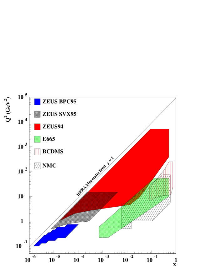
Figure 1: The $(x,Q^{2})$ plane showing the regions covered by the ZEUS data sets BPC95, ZEUS94 and SVX95 together with regions covered by the fixed target experiments E665, BCDMS and NMC.

With data taken during the 1995 HERA run the ZEUS experiment has achieved a significant increase in the kinematic coverage for low $x$ and low $Q^{2}$ inelastic neutral current positron-proton scattering. The coverage for $Q^{2}$ between 0.11 and $0.65\mbox{\hskip 3.00003pt\rm GeV}^{2}$ was made possible with the installation of a small electromagnetic sampling calorimeter, the Beam Pipe Calorimeter (BPC), at small positron scattering angles and results on the proton structure function $F_{2}$ and the total $\gamma^{*}p$ cross-section have been published [2]. In Sec. 3 of this paper we report on further measurements of $F_{2}$ in the $Q^{2}$ range between 0.6 and $17\mbox{\hskip 3.00003pt\rm GeV}^{2}$. The data were obtained from runs in which the interaction point was shifted away from the main rear calorimeter thus extending its small-angle coverage for scattered positrons. These data fill the gap in $Q^{2}$ between the BPC and the 1994 ZEUS measurements [3, 4]. Taking all three data sets together, the ZEUS experiment has measured $F_{2}$ over the kinematic region $0.1<Q^{2}<5000\mbox{\hskip 3.00003pt\rm GeV}^{2}$, $2\times 10^{-6}<x<0.5$. The coverage of the kinematic plane by the ZEUS data sets is shown in Fig. 1.

The very low $Q^{2}$ data are discussed in Sec. 4 using generalised vector dominance and Regge theory and it is established that the ZEUS data with $Q^{2}\leq 0.65\mbox{\hskip 3.00003pt\rm GeV}^{2}$ are well described by such approaches. In Sec. 5 the slopes $dF_{2}/d\ln Q^{2}$ at fixed $x$ and $d\ln F_{2}/d\ln(1/x)$ at fixed $Q^{2}$ are derived from the combined ZEUS data sets. In Sec. 6 the ZEUS $F_{2}$ data, together with fixed target data at large $x$, are fit using next to leading order (NLO) QCD to determine the gluon momentum density. The increased range and precision of the ZEUS $F_{2}$ data allow a more precise extraction of the gluon density at low $x$ compared to our earlier results using the 1993 ZEUS data [5]. In Sec. 7 the properties of the pQCD description of the $F_{2}$ and slopes data at low $Q^{2}$ are explored in more detail. Our conclusions are summarised in Sec. 8. Tables containing $F_{2}$ values and other data are given in the Appendix.

2 Phenomenology of the low $Q^{2}$ region

We use NLO pQCD and the simplest non-perturbative models to explore the transition region in $Q^{2}$. The standard NLO DGLAP equations [6] give the $Q^{2}$ evolution of parton densities, but do not prescribe their functional form in $x$  at the starting scale $Q^{2}_{0}$. At $Q^{2}_{0}$, the small $x$ behaviour of parton momentum densities $xf(x)$ may be characterised by the exponent $\delta$ where $xf(x)\approx Ax^{\delta}$. For $\delta\geq 0$ a parton momentum density either tends to zero or is constant as $x\to 0$ (non-singular) while for $\delta<0$ a parton density increases as $x\to 0$ (singular). One way to understand the rise of $F_{2}$ at low $x$ is advocated by Glück, Reya and Vogt (GRV) [7, 8] who argue that the starting scale for the evolution of the parton densities should be very low ($0.34$ GeV²) and at the starting scale the parton density functions should be non-singular. For $Q^{2}>1\mbox{\hskip 3.00003pt\rm GeV}^{2}$, the observed rise in $F_{2}$ is then generated dynamically through the DGLAP evolution equations. On the other hand, at low $x$ one might expect that the DGLAP equations break down because of large $\ln(1/x)$ terms that are not included. Such terms are taken into account by the BFKL formalism [9], which in leading order predicts a rising $F_{2}$ at low $x$. The rise comes from a singular gluon density with $\delta$ in the range $-0.3$ to $-0.5$. Recent work on BFKL at NLO has shown that the corrections to the LO value for $\delta$ are large [10] and reduce the predicted rise in $F_{2}$, though quite how large the reduction should be is still under discussion [11]. Clearly accurate experimental results on $F_{2}$ and $\delta$ at low $x$ are of great interest. More details on the many alternative pQCD approaches to the low $x$ region may be found in [12, 13].

As $Q^{2}$ decreases $\alpha_{S}$ increases and pQCD will eventually break down. Then non-perturbative models must be used to describe the data. At low $x$ the lifetime of the virtual photon in the proton rest frame is large compared to the $\gamma^{*}p$ interaction time [14]. Inelastic $e^{\pm}p$ scattering may then be viewed as $\gamma^{*}p$ scattering, with the total $\gamma^{*}p$ cross-section given by 

$$\sigma_{\rm tot}^{\gamma^{*}p}(W^{2},Q^{2})\equiv\sigma_{T}+\sigma_{L}\approx\frac{4\pi^{2}\alpha}{Q^{2}}F_{2}(x,Q^{2}),$$ (1)

where $W\approx\sqrt{Q^{2}/x}$ is the centre-of-mass energy of the $\gamma^{*}p$ system and $\sigma_{T}$ and $\sigma_{L}$ are the cross-sections for transversely and longitudinally polarised virtual photons respectively. We consider two non-perturbative approaches, the vector meson dominance model (VMD) and Regge theory.

VMD relates the hadronic interactions of the photon to a sum over interactions of the $\rho^{0},\omega$ and $\phi$ vector meson states [15, 16]. To accommodate deep inelastic scattering data the sum has to be extended to an infinite number of vector mesons giving the generalised vector dominance model (GVMD) [17]. Following the assumptions in [17], $\sigma_{T}(W^{2},Q^{2})$ is related to $\sigma^{\gamma p}(W^{2})$, the total photoproduction cross-section by

$$\sigma_{T}(W^{2},Q^{2})=\left[{r_{C}M_{0}^{2}\over(M_{0}^{2}+Q^{2})}+\sum_{V=\rho^{0},\omega,\phi}{r_{V}M_{V}^{4}\over(M_{V}^{2}+Q^{2})^{2}}\right]\sigma^{\gamma p}(W^{2}),$$ (2)

where $M_{0}$ is the lower cutoff of the continuum vector states and $r_{C},r_{V}$ are constants satisfying the normalisation condition $r_{C}+\sum_{V}r_{V}=1$ at $Q^{2}=0$. A similar expression to Eq. (2) may be written for $\sigma_{L}(W^{2},Q^{2})$, but with additional $Q^{2}$ dependence to ensure that it vanishes as $Q^{2}\to 0$ [17]. The GVMD approach has recently been revived in the context of low $Q^{2}$ HERA data by Schildknecht and Spiesberger [18]. We use a simplified form of GVMD to study the consistency of the data in the ZEUS BPC region and its extrapolation to $Q^{2}=0$.

Regge theory [19, 20] provides a framework in which the energy dependence of hadronic total cross-sections is of the form $\sigma\sim\sum_{r}\beta_{r}s^{\alpha_{r}-1}$ where $\sqrt{s}$ is the centre-of-mass energy, $\alpha_{r}$ the intercept of the Regge trajectory and $\beta_{r}$ a process dependent constant. The $\alpha_{r}$ are universal and can in principle be determined from the spectrum of meson states. However, for the dominant trajectory describing total cross-sections at high energies (known as the Pomeron), this has not yet been possible. The Pomeron intercept, $\alpha_{P}$, is determined by fitting high energy total cross-section data. Donnachie and Landshoff (DL) [21] have used a two component Pomeron+Reggeon approach to give a good description of hadron-hadron and photoproduction total cross-section data over a wide range of energies with $\alpha_{P}$ of about 1.08. They have extended their approach to $\gamma^{*}p$ total cross-sections [22] by keeping the Regge intercept independent of $Q^{2}$ but assuming a simple $Q^{2}$ dependence for the coupling term, which becomes $\beta_{r}m_{r}^{2}/(m_{r}^{2}+Q^{2})$ where $m^{2}_{r}$ is again determined by fitting to data.

Neither the non-perturbative VMD and DL approaches nor pQCD can be expected to describe the $Q^{2}$ behaviour of $F_{2}$ over the complete range from photoproduction to very large $Q^{2}$ deep inelastic scattering (DIS). Many models combining various aspects of these approaches have been applied to the data in the transition region [13, 23, 24]. A comparison of the ZEUS BPC data with some of the models was given in [2]. We use the DL Regge model [22] and the 1994 parton densities (GRV94) of the GRV group [8] as ‘benchmarks’ in this paper as they were available before the recent precision measurements were made.

3 Measurement of $F_{2}$ with shifted vertex data

The shifted vertex data correspond to an integrated luminosity of $236\mbox{\hskip 3.00003pt\rm nb}^{-1}$ taken in a special running period in which the nominal interaction point was offset in the proton beam direction by $+70\mbox{\hskip 3.00003pt\rm cm}$,  i.e. away from the main rear calorimeter (RCAL). The measurement follows previous analyses described in more detail in [3, 4]. However, compared to the earlier shifted vertex analysis [3], for the 1995 data taking period the RCAL modules above and below the beam were moved closer to the beam, thus extending the shifted vertex $Q^{2}$ range down to $0.6\mbox{\hskip 3.00003pt\rm GeV}^{2}$. The basic detector components used are the compensating uranium calorimeter (CAL), which has an energy resolution, as measured in the test beam, of $\sigma/E=18\%/\sqrt{E({\rm GeV})}$ for electromagnetic particles and $\sigma/E=35\%/\sqrt{E({\rm GeV})}$ for hadronic particles. The tracking chamber system is used to determine the position of the event vertex. The small angle rear tracking detector (SRTD) consists of horizontal and vertical scintillator strips covering the region around the RCAL beam hole, i.e. the region of positron scattering angles of low $Q^{2}$ events. It is also used as a preshower detector for the RCAL and has a position resolution of $0.3\mbox{\hskip 3.00003pt\rm cm}$. The luminosity is determined from the positron-proton bremsstrahlung $ep\rightarrow ep\gamma$ where the radiated photon is measured in a lead-scintillator calorimeter (LUMI) positioned at $Z=-107\mbox{\hskip 3.00003pt\rm m}$. There is an associated electron calorimeter (LUMI-E), positioned at $Z=-35\mbox{\hskip 3.00003pt\rm m}$, which is used for tagging photoproduction events. The uncertainty in the luminosity measurement is $1\%$.

3.1 Monte Carlo simulation

Monte Carlo (MC) events are used to correct for the detector acceptance, resolution and the effect of initial state radiation. In the framework of DJANGO [25] the generator HERACLES [26] is used to simulate neutral current DIS events including first order electroweak radiative effects. The hadronic final state is simulated using the ARIADNE [27] program which implements the colour-dipole model. A parameterisation of the $F_{2}$ structure functions based on the results published in [4] is used and $F_{L}$ is set to zero. The MC event sample is 1.6 times that of the data and the events are passed through the same offline reconstruction software as the data. Simulated photoproduction background events are generated using the program PYTHIA [28] with a cross-section given by the ALLM [29] parameterisation.

3.2 Kinematic reconstruction

The reaction $e^{+}(k)+p(P)\rightarrow e^{+}(k^{\prime})+X$ at fixed squared centre-of-mass energy, $s=(k+P)^{2}$, is described in terms of $Q^{2}\equiv-q^{2}=-(k-k^{\prime})^{2}$ and Bjorken $x=Q^{2}/(2P\cdot q)$. At HERA $s\approx 4E_{e}E_{p}$, where $E_{e}=27.5\mbox{\hskip 3.00003pt\rm GeV}$ and $E_{p}=820\mbox{\hskip 3.00003pt\rm GeV}$ denote the positron and proton beam energies. The fractional energy transferred to the proton in its rest frame is $y=Q^{2}/(sx)$.

The kinematic variables are reconstructed from the measured energy, $E_{e}^{\prime}$, and scattering angle, $\theta_{e}$, of the positron (the ‘electron method’),

$$Q^{2}=2E_{e}E_{e}^{\prime}\left(1+\cos\theta_{e}\right)\,\,\,{\rm and}\,\,\,y=1-\frac{E_{e}^{\prime}}{2E_{e}}\left(1-\cos\theta_{e}\right).$$

This method gives the best resolution in the region of interest at high $y$ and low $Q^{2}$.

Scattered positrons are identified by a neural network based algorithm [4], with an efficiency of about 90% at positron energies of $10\mbox{\hskip 3.00003pt\rm GeV}$, increasing to $100\%$ at $20\mbox{\hskip 3.00003pt\rm GeV}$. The measured energy is corrected for energy loss in inactive material in front of the CAL using the signals in the SRTD scintillators. The uncertainty in the measured energy is estimated to be $2\%$ at $10\mbox{\hskip 3.00003pt\rm GeV}$ decreasing to $1\%$ at $27.5\mbox{\hskip 3.00003pt\rm GeV}$. The positron impact position on the CAL measured with the SRTD together with the event vertex position measured with tracks in the CTD gives the positron scattering angle $\theta_{e}$. For events outside the fiducial volume of the SRTD, the CAL position determination is used. For events in which the event vertex cannot be reconstructed, the vertex is set to the mean value of the vertex distribution.

The variable $y_{\rm JB}=\sum_{i}E_{i}(1-\cos\theta_{i})/(2E_{e})$, where the sum runs over all CAL cells except those belonging to the scattered positron, gives a measurement of $y$ with a good resolution at low $y$. A cut $y_{\rm JB}>0.04$ is imposed to limit event migrations from low $y$, where the resolution of the electron method is poor, into the bins at higher $y$.

3.3 Event selection

Data are selected online by a three level trigger system. At the first level a certain energy deposit in the CAL is required and cuts on the arrival times of particles measured in the SRTD are imposed. At the second level the condition $\delta\equiv\sum_{i}E_{i}(1-\cos\theta_{i})>29\mbox{\hskip 3.00003pt\rm GeV}-2E_{\gamma}$ has to be fulfilled, where the sum goes over all CAL cells with energies $E_{i}$ and polar angles $\theta_{i}$, and $E_{\gamma}$ is the energy measured in the LUMI detector. This cut significantly reduces the photoproduction background as $\delta=2E_{e}$ ($55\mbox{\hskip 3.00003pt\rm GeV}$) for a fully contained DIS event. At the third level a full event reconstruction is performed. A reconstructed positron with an energy greater than $4\mbox{\hskip 3.00003pt\rm GeV}$ and a CAL impact point outside a box of $24(X)\mbox{\hskip 3.00003pt\rm cm}\times 12(Y)\mbox{\hskip 3.00003pt\rm cm}$ centered on the RCAL beam hole is required. Also, $\delta$ has to be greater than $30\mbox{\hskip 3.00003pt\rm GeV}$ and event times measured in the CAL are required to be consistent with an $e^{+}p$ interaction at the nominal shifted interaction point.

The offline event selection cuts are:

• Positron finding as described above, including the requirements on the impact point and on $y_{\rm JB}>0.04$, with a corrected positron energy $E_{e}^{\prime}>10\mbox{\hskip 3.00003pt\rm GeV}$. This ensures a high efficiency for positron finding and removes events at very high $y$, which suffer from large photoproduction backgrounds.

• The positron impact point on the CAL is required to be outside a box of $26\mbox{\hskip 3.00003pt\rm cm}\times 16\mbox{\hskip 3.00003pt\rm cm}$ around the RCAL beam pipe hole to ensure full shower containment in the CAL.

• $35\mbox{\hskip 3.00003pt\rm GeV}<\delta<65\mbox{\hskip 3.00003pt\rm GeV}$, in order to further reduce photoproduction and beam-gas related backgrounds. This cut also removes events with hard initial state radiation.

• For events with a tracking vertex, the reconstructed $Z$ coordinate of the vertex is required to lie within $40\mbox{\hskip 3.00003pt\rm cm}<Z_{\rm vertex}<160\mbox{\hskip 3.00003pt\rm cm}$. The acceptance is extended to large $Z$ values to accommodate events from satellite bunches, i.e. proton bunches that are shifted by $4.8\mbox{\hskip 3.00003pt\rm ns}$ with respect to the primary bunch crossing time, resulting in a fraction of $ep$ interactions occurring displaced by an additional $72\mbox{\hskip 3.00003pt\rm cm}$.

A total of 62000 events pass the cuts.

3.4 Background estimation

The background from beam-gas interactions is about 1% as determined from unpaired positron and proton bunches.

The main background comes from photoproduction events, where the positron escapes along the beam line and a mis-identified positron (mainly electromagnetic showers from $\pi^{0}$ decays) is reconstructed in the CAL. The amount of this background is determined using the MC simulated photoproduction event sample. In total it is a small effect which is only significant at small values of $E^{\prime}_{e}$ and $Q^{2}$ as shown in plots (d) and (e) of Fig. 2. In a small fraction of real photoproduction events the positron is detected inside the limited acceptance of the LUMI-E electron tagger. These events are used to cross check the MC background estimate. Both results agree within 20%.

3.5 Determination of $F_{2}$

In the $Q^{2}$ range of this analysis the double differential cross-section for single virtual-photon exchange in DIS is given by

$$\frac{d^{2}\sigma}{dxdQ^{2}}=\frac{2\pi\alpha^{2}}{xQ^{4}}\left[2\left(1-y\right)+\frac{y^{2}}{1+R}\right]F_{2}(x,Q^{2})\left[1+\delta_{r}(x,Q^{2})\right],$$ (3)

where $R$ is related to the longitudinal structure function $F_{L}$ by $R=F_{L}/(F_{2}-F_{L})$ and $\delta_{r}$ gives the radiative correction to the Born cross-section. For the kinematic range of this analysis $\delta_{r}$ is at most $10\%$. For $R$ we take values given by the BKS model [30]. An iterative procedure is used to extract the structure function $F_{2}$. Data and MC events are binned in the variables $y$ and $Q^{2}$. In a bin-by-bin unfolding procedure the MC differential cross-section is adjusted to describe the data using a smooth function for $F_{2}$. The re-weighted MC events are then used to unfold $F_{2}$ again, until after 3 iterations the changes to $F_{2}$ are below $0.5\%$. The statistical errors of the $F_{2}$ values are calculated from the number of events measured in a bin and the statistical error on the acceptance calculation from the MC simulation.

The quality of the description of the data by the re-weighted MC is shown in Fig. 2, which displays distributions of the following quantities: (a) $\delta$ or $E-P_{Z}$ as defined in Sec. 3.3; (b) the $Z$-position of the primary vertex; (c) the positron scattering angle $\theta_{e}$; (d) the energy, $E^{\prime}_{e}$, of the scattered positron; (e) $\log_{10}Q^{2}$; (f) $\log_{10}y$. The agreement between data (filled circles) and simulated data (open histograms, normalised to the luminosity of the data) is generally good.

3.6 Systematic uncertainties

The systematic uncertainties of the measured $F_{2}$ values are determined by changing the selection cuts or the analysis procedure in turn and repeating the extraction of $F_{2}$. Positive and negative differences, $\Delta F_{2}$, are added in quadrature separately to obtain the total positive and negative systematic errors. The systematic checks and errors are:

• A shift of the horizontal and vertical position of the SRTD by $\pm 0.5\mbox{\hskip 3.00003pt\rm mm}$ results in $\Delta F_{2}/F_{2}$ of at most $\approx 2\%$.

• The two halves of the SRTD are moved with respect to each other in the horizontal and vertical directions by $1.0\mbox{\hskip 3.00003pt\rm mm}$, which results in $\Delta F_{2}/F_{2}$ of $\approx 4\%$.

• The uncertainty in the positron energy calibration is estimated to be $2\%$ at $10\mbox{\hskip 3.00003pt\rm GeV}$ decreasing to $1\%$ at $27.5\mbox{\hskip 3.00003pt\rm GeV}$ giving a maximum $\Delta F_{2}/F_{2}$ of $8\%$.

• The hadron energy scale is uncertain to $\pm 3\%$, causing a maximum $\Delta F_{2}/F_{2}$ of 2%.

• The uncertainty in the positron finder efficiency is estimated to be $2.5\%$ at $10\mbox{\hskip 3.00003pt\rm GeV}$ decreasing to $1\%$ at $27.5\mbox{\hskip 3.00003pt\rm GeV}$, which gives $\Delta F_{2}/F_{2}$ of at most 2%.

• The number of MC events in satellite bunches is increased by 100% and decreased to 50%. This leads to a $\Delta F_{2}/F_{2}$ less than 2%.

• The uncertainty in the determination of the photoproduction background by MC is estimated to be $30\%$. The resulting maximum $\Delta F_{2}/F_{2}$ is about 7% in the highest $y$ bins.

• The vertex finding efficiency is between 75% and 95% depending on the kinematic region. To study the effect of differences in the efficiency between MC and data all vertices are assigned to the nominal interaction point. $\Delta F_{2}/F_{2}$ is at most 6%.

• A variation in the box cut from $26\mbox{\hskip 3.00003pt\rm cm}\times 16\mbox{\hskip 3.00003pt\rm cm}$ to $25.6\mbox{\hskip 3.00003pt\rm cm}\times 15.6\mbox{\hskip 3.00003pt\rm cm}$ or $26.4\mbox{\hskip 3.00003pt\rm cm}\times 8.4\mbox{\hskip 3.00003pt\rm cm}$, giving a maximum change $\Delta F_{2}/F_{2}$ of 7%.

The acceptance for DIS events with a rapidity gap at low $Q^{2}$ is somewhat different from that of non-diffractive events due to the different energy flow. To check the effect on $F_{2}$, the acceptance for diffractive events is first calculated using a separate diffractive MC. Using this and the measured fraction of rapidity gap events in each bin, the acceptance function is recalculated. The largest change to $F_{2}$ is $2.5\%$. The data are corrected for this effect. Half the correction value is taken as the estimate of the systematic error, reflecting mainly the uncertainty in the fraction of diffractive events.

In addition there is an overall normalisation uncertainty of 1.5%, due to the 1% error in the luminosity measurement and a 1% uncertainty in the trigger efficiency, which is not included in the point to point systematic error estimate.

The $F_{2}$ data cover the $x$ range $1.2\times 10^{-5}-1.9\times 10^{-3}$ in 12 bins of $Q^{2}$ between 0.6 and $17\mbox{\hskip 3.00003pt\rm GeV}^{2}$ (ZEUS SVX95). The values for $F_{2}$ and their systematic errors are given in Table 1 of the Appendix. Fig. 3 shows the results for $F_{2}$ as a function of $x$ in the 12 $Q^{2}$ bins. In the lowest $Q^{2}$ bin data from ZEUS $F_{2}$ measurements at very low $Q^{2}$ using the BPC (BPC95) [2] are shown and at larger $Q^{2}$ those from the ZEUS94 measurements [4]. Also shown are data from the shifted vertex measurements by H1 (H1 SVX95) [31] and fixed target data from E665 [32]. There is good agreement between the different ZEUS data sets and between ZEUS, E665 and H1 data in the regions of overlap. We note that the steep increase of $F_{2}$ at low $x$ observed in the higher $Q^{2}$ bins softens at the lowest $Q^{2}$ values. The curves shown will be discussed later.

4 The low $Q^{2}$ region

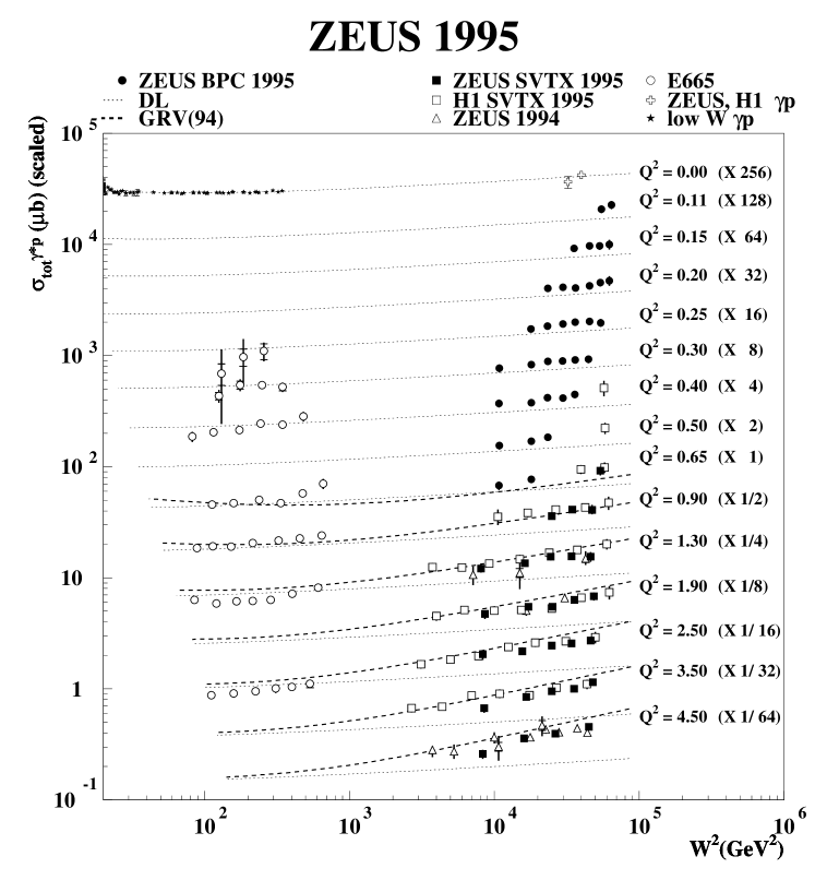
Figure 4: The total $\gamma^{*}p$ cross-section, $\sigma_{\rm tot}^{\gamma^{*}p}$, as a function of $W^{2}$ at different $Q^{2}$ [GeV²]. The data of this analysis (ZEUS SVX95) are shown together with previous ZEUS and H1 data (ZEUS94, ZEUS BPC95, H1 SVX95). Also the total photoproduction cross-sections from ZEUS and H1 and from fixed target experiments at lower $W$ are shown. Predictions from the DL [22] and GRV94 [8] models are indicated by the dotted and dashed curves, respectively.

We first give an overview of the $Q^{2}\leq 4.55\mbox{\hskip 3.00003pt\rm GeV}^{2}$ region. Fig. 4 shows the ZEUS cross-section data versus $W^{2}$ derived from the SVX95, BPC95 and ZEUS94 $F_{2}$ values using Eq. (1). Also shown are data from H1 SVX95 and measurements of the total cross-section for scattering of real photons on protons at fixed target [33] and HERA energies [34]. The two curves shown are the predictions of the DL Regge model [22] and $\sigma_{\rm tot}^{\gamma^{*}p}$ calculated from the NLO QCD parton distributions of GRV94 [8]. The DL model predicts that the cross-section rises slowly with energy $\propto W^{2\lambda}$, $\lambda=1-\alpha_{P}\approx 0.08$ and this behaviour seems to be followed by the data at very low $Q^{2}$ values, although the normalisation of the DL model is low compared to the ZEUS BPC95 data. Above $Q^{2}=0.65\mbox{\hskip 3.00003pt\rm GeV}^{2}$, the DL model predicts a shallower rise of the cross-section than the data exhibit. For $Q^{2}$ values around $1\mbox{\hskip 3.00003pt\rm GeV}^{2}$ and above, the GRV94 curves describe the qualitative behaviour of the data, namely the increasing rise of $\sigma_{\rm tot}^{\gamma^{*}p}$ with $W^{2}$, as $Q^{2}$ increases. This suggests that the pQCD calculations can account for a significant fraction of the cross-section at the larger $Q^{2}$ values.

For the remainder of this section we concentrate on non-perturbative descriptions of the ZEUS BPC95 data ($0.11<Q^{2}<0.65\mbox{\hskip 3.00003pt\rm GeV}^{2}$). Since the BPC data are binned in $Q^{2}$ and $y$ we first rewrite the double differential cross-section of Eq. (3) (dropping the radiative correction factor) as

$${d^{2}\sigma\over dydQ^{2}}=\Gamma\cdot(\sigma_{T}+\epsilon\sigma_{L})$$ (4)

where $\displaystyle\sigma_{L}={Q^{2}\over 4\pi^{2}\alpha}F_{L}$ and $\sigma_{T}+\sigma_{L}$ has been defined by Eq. (1). The virtual photons have flux $\Gamma=\alpha(1+(1-y)^{2})/(2\pi Q^{2}y)$ and polarisation $\epsilon=2(1-y)/(1+(1-y)^{2})$. For the BPC data $\epsilon$ lies in the range $0.55-0.99$ but as $s$ is fixed at HERA, $\epsilon$ cannot be varied independently of $x$ and $Q^{2}$. Thus the experimently determined quantity is the combination $\sigma_{T}+\epsilon\sigma_{L}$. For simplicity we keep only the continuum term in the GVMD expression of Eq. (2). At a fixed $W$ the longitudinal and transverse $\gamma^{*}p$ cross-sections are then related to the corresponding cross-section $\sigma_{0}^{\gamma p}$ at $Q^{2}=0$ by

$$\sigma_{L}(W^{2},Q^{2}) = \xi\left[\frac{M_{0}^{2}}{Q^{2}}\ln\frac{M_{0}^{2}+Q^{2}}{M_{0}^{2}}-\frac{M_{0}^{2}}{M_{0}^{2}+Q^{2}}\right]\sigma_{0}^{\gamma p}(W^{2})$$

$$\sigma_{T}(W^{2},Q^{2}) = \frac{M_{0}^{2}}{M_{0}^{2}+Q^{2}}\sigma_{0}^{\gamma p}(W^{2}),$$ (5)

where the parameter $\xi$ is the ratio $\sigma_{L}^{Vp}/\sigma_{T}^{Vp}$ for vector meson (V) proton scattering and $M_{0}$ is the effective vector meson mass. Neither $\xi$ nor $M_{0}$ are given by the model and they are usually determined from data. We set $\sigma_{L}$ to zero because $\xi$ is expected to be less than one  and the factor in the square bracket in the expression for $\sigma_{L}$ is small (for $Q^{2}\leq 0.65\mbox{\hskip 3.00003pt\rm GeV}^{2}$ and $M_{0}\approx m_{\rho}$, it is less than 0.2). The $Q^{2}$ dependence of the BPC data, in 8 bins of $W$ between 104 and $251\mbox{\hskip 3.00003pt\rm GeV}$, is fit with a single mass parameter $M_{0}^{2}$. The cross-sections, $\sigma_{0}^{\gamma p}(W^{2})$, are also fit at each $W$ giving a total of 9 parameters. The fit is reasonable ($\chi^{2}/ndf=38.7/(34-9)=1.55$, statistical errors only) as shown in the upper plot of Fig. 5. To estimate the systematic errors, the fit is first repeated for each systematic check on the BPC data, using data and statistical errors corresponding to that change. The systematic errors are then determined by adding in quadrature the changes from the nominal values of the parameters. As a final check on the stability of the results, the fit is repeated including the longitudinal term with $\xi=0.4$. The resulting changes in the values for the cross-sections are less than their statistical errors (more details are given in [36]). The value obtained for $M_{0}^{2}$ is $0.53\pm 0.04({\rm stat})\pm 0.09({\rm sys})\mbox{\hskip 3.00003pt\rm GeV}^{2}$. The resulting extrapolated values of $\sigma_{0}^{\gamma p}$ are given in Table 2 of the Appendix and shown as a function of $W^{2}$ in the lower plot of Fig. 5, along with measurements from HERA and lower energy experiments. The BPC $\sigma_{0}^{\gamma p}$ values lie somewhat above the direct measurements from HERA. They are also above the prediction of Donnachie and Landshoff. It should be clearly understood that the $\sigma_{0}^{\gamma p}$ values derived from the BPC are not a measurement of the total photoproduction cross-section but the result of a phenomenologically motivated extrapolation.

The simple GVMD approach just described gives a concise account of the $Q^{2}$ dependence of the BPC data. To describe the energy dependence of the data we use a two component Regge model

$$\sigma_{\rm tot}^{\gamma p}(W^{2})=A_{R}(W^{2})^{\alpha_{R}-1}+A_{P}(W^{2})^{\alpha_{P}-1}$$

where $P$ and $R$ denote the Pomeron and Reggeon contributions. The Reggeon intercept $\alpha_{R}$ is fixed to the value $0.5$ which is compatible with the original DL value [21], and recent estimates [37, 38]. Fitting only the Pomeron term to the extrapolated BPC data ($\sigma_{0}^{\gamma p}$) gives $\alpha_{P}=1.141\pm 0.020$(stat)$\pm 0.044$(sys). Fitting both terms to the real photoproduction data (with $W^{2}>3\mbox{\hskip 3.00003pt\rm GeV}^{2}$) and BPC $\sigma_{0}^{\gamma p}$ data yields $\alpha_{P}=1.101\pm 0.002$(stat)$\pm 0.012$(sys). Including, in addition, the two direct measurements from HERA [34] gives $\alpha_{P}=1.100\pm 0.002$(stat)$\pm 0.012$(sys). At HERA energies the contribution of the Reggeon term is negligible. The values of $\alpha_{P}$ are compatible with the DL value of 1.08 and the recent best estimate of $1.0964^{+0.0115}_{-0.0094}$ by Cudell et al. [38].

The final step in the analysis of the BPC data is to combine the $Q^{2}$ dependence from the GVMD fit with the energy dependence from the Regge model

$$\sigma_{\rm tot}^{\gamma^{*}p}(W^{2},Q^{2})=\left({M_{0}^{2}\over M_{0}^{2}+Q^{2}}\right)(A_{R}(W^{2})^{\alpha_{R}-1}+A_{P}(W^{2})^{\alpha_{P}-1}).$$ (6)

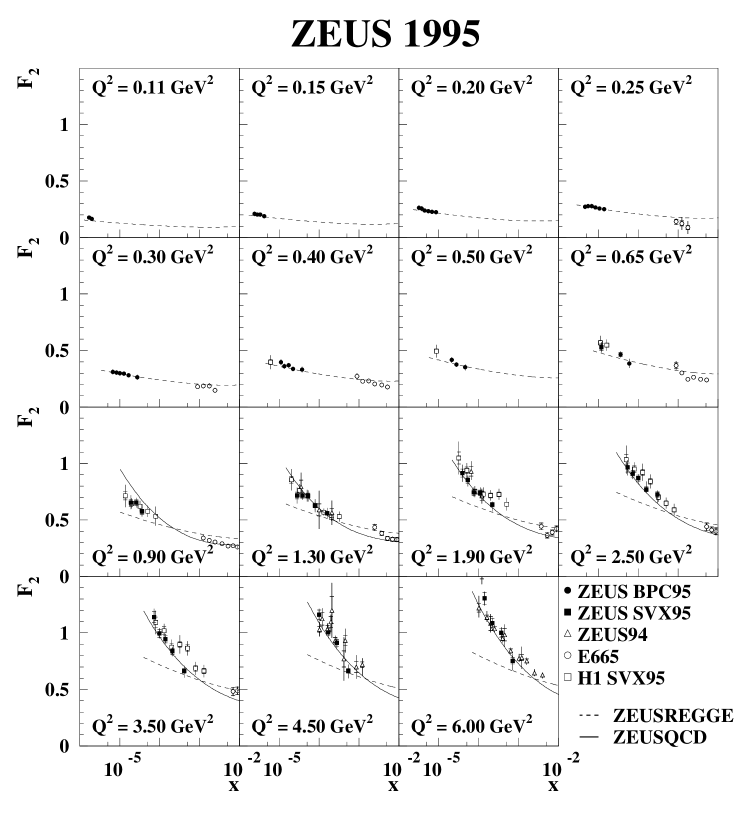
Figure 6: Low $Q^{2}$ $F_{2}$ data for different $Q^{2}$ bins together with the ZEUS Regge fit (dashed curves) to the BPC95 data as described in Sec. 4. Also shown at larger values of $Q^{2}$ is the ZEUS NLO QCD fit (full curves) as described in Sec. 6.

The parameter $M_{0}^{2}$ is fixed to its value of $0.53$ found above and $\alpha_{R}$ is also kept fixed at 0.5 as before. The 3 remaining parameters are determined by fitting to photoproduction data (with $W^{2}>3\mbox{\hskip 3.00003pt\rm GeV}^{2}$, but without the two original HERA measurements ) and the measured BPC data. We find $A_{R}=145.0\pm 2.0\,\mu$b, $A_{P}=63.5\pm 0.9\,\mu$b and $\alpha_{P}=1.097\pm 0.002$ with $\chi^{2}/ndf=1.12$ (statistical errors only). If the two HERA photoproduction measurements are included the parameters do not change within their errors. The description of the low $Q^{2}$ $F_{2}$ data given by this model (ZEUSREGGE) is shown in Fig. 6. Data in the BPC region $Q^{2}\leq 0.65\mbox{\hskip 3.00003pt\rm GeV}^{2}$ are well described. At larger $Q^{2}$ values the curves fall below the data. Including ZEUS SVX95 data at successively larger $Q^{2}$ values, we find that by $Q^{2}=3.5\mbox{\hskip 3.00003pt\rm GeV}^{2}$ the $\chi^{2}/ndf$ has increased to 1.7. Also shown in Fig. 6, for $Q^{2}\geq 0.9\mbox{\hskip 3.00003pt\rm GeV}^{2}$, are the results of a NLO QCD fit (ZEUSQCD) described in Sec. 6.

To summarise, we have shown that the $Q^{2}$ dependence of the ZEUS BPC95 data at very low $Q^{2}$ can be described by a simple GVMD form. The resulting values of $\sigma_{0}^{\gamma p}$, the cross-sections extrapolated to $Q^{2}=0$, are somewhat larger than the direct measurements at HERA. A two component Regge model gives a good description of the $W^{2}$ dependence of the data, with a Pomeron intercept compatible with that determined from hadron-hadron data.

5 $F_{2}$ slopes

To quantify the low $x$ behaviour of $F_{2}$ as a function of $x$ and $Q^{2}$, we calculate the slopes $d\ln F_{2}/d\ln(1/x)$ at fixed $Q^{2}$ and $dF_{2}/d\ln Q^{2}$ at fixed $x$ from the ZEUS SVX95, BPC95 and ZEUS94 data sets. We use the ALLM97 parameterisation [39] for bin-centering $F_{2}$ data when necessary.

5.1 The slope $d\ln F_{2}/d\ln(1/x)$

It is seen from Fig. 6 that the $x$ slope of $F_{2}$ is small for small $Q^{2}$ and then starts to increase as $Q^{2}$ increases. At a fixed value of $Q^{2}$ and at small $x$ the behaviour of $F_{2}$ can be characterised by $F_{2}\propto x^{-\lambda_{eff}}$ (giving $\lambda_{eff}=d\ln F_{2}/d\ln(1/x)$), with $\lambda_{eff}$ taking rather different values in the Regge and LO BFKL approaches. The value of $\lambda_{eff}$ as an observable at small $x$ has been discussed by Navelet et al. [40, 41] and data on $\lambda_{eff}$ with $x<0.1$ have been presented by H1 [42].

Using statistical errors only, we fit $F_{2}$ data at fixed $Q^{2}$ and $x<0.01$ to the form $Ax^{-\lambda_{eff}}$. Refering to Fig. 1, we are measuring $\lambda_{eff}$ from horizontal slices of $F_{2}$ data between the $y=1$ HERA kinematic limit and the fixed cut of $x<0.01$. As the $x$ range of the ZEUS BPC95 data is restricted we include data from E665 [32]. In each $Q^{2}$ bin the average value of $x$, $\langle x\rangle$, is calculated from the mean value of $\ln(1/x)$ weighted by the statistical errors of the corresponding $F_{2}$ values in that bin. For the estimation of the systematic errors, it is assumed that the systematic error analyses for each of the four data sets used are independent. For a particular data set and a given systematic check, the $F_{2}$ points in each $Q^{2}$ bin are moved up and down by the respective systematic error estimates and the fits repeated, keeping all other data sets fixed at their nominal values. The positive and negative shifts with respect to the central values of $\lambda_{eff}$ are added separately in quadrature to give the positive and negative systematic errors.

Fig. 7 shows the measured values of $\lambda_{eff}$ as a function of $Q^{2}$, and the data are given in Table 3 of the Appendix. At very low $Q^{2}$ the errors on $\lambda_{eff}$ are large because this region is below the lower limit of E665 data (see Fig. 1). At $Q^{2}>100\mbox{\hskip 3.00003pt\rm GeV}^{2}$ the statistical error dominates. From the Regge approach of the previous section one would expect $\lambda_{eff}\approx 0.1$, independently of $Q^{2}$. Data for $Q^{2}<1\mbox{\hskip 3.00003pt\rm GeV}^{2}$ are consistent with this expectation. The points labelled DL, linked by a dashed line, are calculated from the Donnachie-Landshoff prediction [22] and as expected from the discussion of the previous section are somewhat below the data. The variation of the DL points with $Q^{2}$ is a consequence of averaging the model in a $Q^{2}$ bin over a variable range of $x$ and hence $W^{2}$. For $Q^{2}>1\mbox{\hskip 3.00003pt\rm GeV}^{2}$, $\lambda_{eff}$ increases to around $0.3$ at $Q^{2}$ values of $40\mbox{\hskip 3.00003pt\rm GeV}^{2}$. Qualitatively the tendency of $\lambda_{eff}$ to increase with $Q^{2}$ is described by a number of pQCD approaches [41]. The points labelled GRV94, linked by a dashed line, are calculated from the NLO QCD GRV94 fit. Although the GRV94 prediction follows the trend of the data it tends to lie above the data, particularly in the $Q^{2}$ range $3-20\mbox{\hskip 3.00003pt\rm GeV}^{2}$. We shall return to this point later. For the predictions shown in Fig. 7 the same $F_{2}$ error weighted average in $x$ at a given $Q^{2}$ is used as for the data.

5.2 The slope $dF_{2}/d\ln Q^{2}$

In QCD the scaling violations of $F_{2}$ are caused by gluon bremsstrahlung from quarks and quark pair creation from gluons. In the low $x$ domain accessible at HERA the latter process dominates the scaling violations. $F_{2}$ is then largely determined by the sea quarks $F_{2}\sim xS$, whereas the $dF_{2}/d\ln Q^{2}$ is dominated by the convolution of the splitting function $P_{qg}$ and the gluon density: $dF_{2}/d\ln Q^{2}\sim\alpha_{S}P_{qg}\otimes xg$. This has been used by Prytz [43] to relate $xg$ directly to the measured values of $dF_{2}/d\ln Q^{2}$ [5]. The importance of $dF_{2}/d\ln Q^{2}$ as a tool for studying the low $x$ region was pointed out by Bartels et al. [44].

In order to study the scaling violations of $F_{2}$ in more detail the logarithmic slope $dF_{2}/d\ln Q^{2}$ is derived from the data by fitting $F_{2}=a+b\ln{Q^{2}}$ in bins of fixed $x$, using only statistical errors. The ZEUS data sets used are the BPC95, SVX95 and ZEUS94. For compatibility with our NLO QCD fit a cut of $W^{2}>10\mbox{\hskip 3.00003pt\rm GeV}^{2}$ is applied to the data. The $F_{2}$ data are shown in bins of $x$ as functions of $Q^{2}$ in Fig. 8. The fits $F_{2}=a+b\ln Q^{2}$ are also shown and the change of slope as $x$ changes is visible from the plots. In each $x$ bin the average value of $Q^{2}$, $\langle Q^{2}\rangle$, is derived from the $F_{2}$ statistical error weighted mean value of $\ln Q^{2}$ in that bin. Systematic errors on $dF_{2}/d\ln Q^{2}$ are estimated following the procedure outlined in the previous section. The results for $dF_{2}/d\ln Q^{2}$ as a function of $x$ are shown in Fig. 9 and are given in Table 4 of the Appendix. The differences in the sizes of the errors on $dF_{2}/d\ln Q^{2}$ partially reflect the variations in $Q^{2}$ range as $x$ varies (see Fig. 1 - we are taking vertical slices of the data to determine $dF_{2}/d\ln Q^{2}$). For values of $x$ down to $3\times 10^{-4}$, the slopes are increasing as $x$ decreases. At lower values of $x$ and $Q^{2}$, the slopes decreases. If $dF_{2}/d\ln Q^{2}$ values are plotted for fixed target data at similar values of $Q^{2}$, the ‘turn over’ is not seen, but the data are at larger values of $x$ [45, 46]. The points linked by the dashed lines are again from the DL Regge model and the GRV94 QCD fit, in both cases calculated using the same $F_{2}$ error weighted $Q^{2}$ averaging as for the data. The failure of DL is in line with our earlier discussion but the fact that GRV94 does not follow the trend of the data when it turns over is perhaps more surprising. Naively it appears that the GRV94 gluon density is too large even at $Q^{2}$ values around $5\mbox{\hskip 3.00003pt\rm GeV}^{2}$. We shall return to this discussion after we have presented the ZEUS NLO QCD fit to which we now turn.

6 NLO QCD fit to $F_{2}$ data and extraction of the gluon momentum density

In this section we present a NLO QCD fit to the ZEUS94 data [4] and the SVX95 data of this paper. We do not attempt a global fit to parton densities, but concentrate on what ZEUS data allow us to conclude about the behaviour of the gluon and quark densities at low $x$.

To constrain the fits at high $x$, proton and deuteron $F_{2}$ structure function data from NMC [47] and BCDMS [48] are included. The following cuts are made on the ZEUS and the fixed target data: (i) $W^{2}>10$ GeV² to reduce the sensitivity to target mass [49] and higher twist [50] contributions which become important at high $x$ and low $Q^{2}$; (ii) discard deuteron data with $x>0.7$ to eliminate possible contributions from Fermi motion in deuterium [51]. The kinematic range covered by the data input to the QCD fit is $3\times 10^{-5}<x<0.7$ and $1<Q^{2}<5000$ GeV².

The QCD predictions for the $F_{2}$ structure functions are obtained by solving the DGLAP evolution equations [6] at NLO in the $\overline{\rm{MS}}$  scheme [52]. These equations yield the quark and gluon momentum distributions (and thus the structure functions) at all values of $Q^{2}$ provided they are given as functions of $x$ at some input scale $Q^{2}_{0}$. In this analysis we adopt the so-called fixed flavour number scheme where only three light flavours ($u,d,s$) contribute to the quark density in the proton. In this scheme the assumption is made that the charm and bottom quarks are produced in the hard scattering process and the corresponding structure functions $F_{2}^{c}$ and $F_{2}^{b}$ are calculated from the photon-gluon fusion process including NLO corrections [53].

As will be explained later, the input scale is chosen to be $Q^{2}_{0}=7$ GeV². The gluon distribution ($xg$), the sea quark distribution ($xS$) and the difference of up and down quarks in the proton ($x\Delta_{ud}$) are parameterised as

$$xg(x,Q_{0}^{2}) = A_{g}x^{\delta_{g}}(1-x)^{\eta_{g}}(1+\gamma_{g}x)$$

$$xS(x,Q_{0}^{2}) \equiv 2x(\bar{u}+\bar{d}+\bar{s})=A_{s}x^{\delta_{s}}(1-x)^{\eta_{s}}(1+\varepsilon_{s}\sqrt{x}+\gamma_{s}x)$$ (7)

$$x\Delta_{ud}(x,Q_{0}^{2}) \equiv x(u+\bar{u})-x(d+\bar{d})=A_{\Delta}x^{\delta_{\Delta}}(1-x)^{\eta_{\Delta}}.$$

The input valence distributions $xu_{v}=x(u-\bar{u})$ and $xd_{v}=x(d-\bar{d})$ at $Q^{2}_{0}$ are taken from the parton distribution set MRS(R2) [54]. As for MRS(R2) we assume that the strange quark distribution is a given fraction $K_{s}=0.2$ of the sea at the scale $Q^{2}=1$ GeV². The gluon normalisation, $A_{g}$, is fixed by the momentum sum rule, $\displaystyle\int^{1}_{0}(xg+xS+xu_{v}+xd_{v})dx=1$. There are thus 11 free parameters in the fit.

The input value for the strong coupling constant is set to $\alpha_{s}(M_{Z}^{2})=0.118$ [55]. With a charm (bottom) threshold of $Q_{c(b)}=1.5$ (5) GeV this corresponds to values of the QCD scale parameter $\Lambda_{\mbox{$\overline{\rm{MS}}$}\ }=(404,343,243)$ MeV for $f=(3,4,5)$ flavours. In the calculation of the charm structure function $F_{2}^{c}$ the charm mass is taken to be $m_{c}=1.5$ GeV; the contribution from bottom is found to be negligible in the kinematic range covered by the data. In the QCD evolutions and the evaluation of the structure functions the renormalisation scale and the mass factorisation scale are both set equal to $Q^{2}$.

The QCD evolutions and the structure function calculations are done with the program QCDNUM [56]. The QCD evolution equations are written in terms of quark flavour singlet and non-singlet and gluon momentum distributions. The quark non-singlet evolution is independent of the gluon. The quark singlet distribution is defined as the sum over all quark and anti-quark distributions

$$x\Sigma=\sum_{i=u,d,s}[xq_{i}(x)+x\bar{q}_{i}(x)]$$ (8)

and its evolution in $Q^{2}$ is coupled to that of the gluon distribution. At small values of $x$, $x\Sigma$ is dominated by the contribution from the $q\bar{q}$ sea $xS$. Note that for data with $Q^{2}<Q^{2}_{0}=7\mbox{\hskip 3.00003pt\rm GeV}^{2}$, backwards evolutions in $Q^{2}$ are performed. The $\chi^{2}$ minimisation and the calculation of the covariance matrices are based on MINUIT [57]. In the definition of the $\chi^{2}$ only statistical errors are included and the relative normalisations of the data sets are fixed at unity.

The fit yields a good description of the data as shown in Fig. 10 where we plot the $Q^{2}$ dependence of the proton structure function $F_{2}$ in the $x$ range covered by the ZEUS94 data. The characteristic pattern of scaling violations can be seen clearly from this plot, with $F_{2}$ at low values of $x$ rising as $Q^{2}$ increases. The quality of the fit to ZEUS data at low $Q^{2}$ is also shown by the full line in Fig. 3. Adding the statistical and systematic errors in quadrature gives a $\chi^{2}$ of 1474 for 1120 data points and 11 free parameters. We have also checked that the gluon obtained from this fit to scaling violations gives values of $F_{2}^{c}$ in agreement with the ZEUS measurements [58]. The values of the fitted parameters are given in Table 5 of the Appendix.

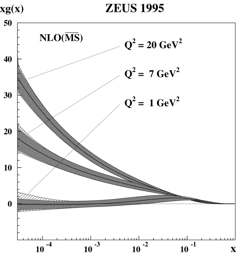
Figure 11: The gluon momentum distribution $xg(x)$ as a function of $x$ at fixed values of $Q^{2}=1$, 7 and 20 GeV² from the ZEUS QCD fit. The inner shaded bands show the ‘HERA standard’ errors of Sec. 6. The outer hatched bands indicate the quadratic sum of the ‘HERA standard’ and the ‘parameterisation’ errors.

Fig. 11 shows the gluon momentum distribution as a function of $x$ for $Q^{2}$ at 1, 7 and $20\mbox{\hskip 3.00003pt\rm GeV}^{2}$. The following sources contribute to the inner shaded error bands displayed in the figure (for each source we give in brackets the relative error $\Delta g/g$ at $x=5\times 10^{-5}$, $Q^{2}=7$ GeV²):

1. The statistical error on the data (4%).

2. The experimental systematic errors, (13%), which are propagated to the covariance matrix of the fitted parameters using the technique described in [59]. In total 26 independent sources of systematic error are included. Proper account is taken of the correlations between the systematic errors of the NMC datasets and for BCDMS the procedure of [50] is followed. Normalisation errors of all data sets are also included.

3. The uncertainties on the strong coupling constant $\Delta\alpha_{s}(M_{Z}^{2})=0.005$ (8%), on the strange quark content of the proton $\Delta K_{s}=0.1$ (1%) and on the charm mass $\Delta m_{c}=0.2$ GeV (1%).

Adding errors from (1), (2) and (3) together in quadrature gives a total contribution of 16%.

In addition to the above sources of error a ‘parameterisation error’ (10%) is obtained by repeating the fit with:

1. The addition of statistical and systematic errors in quadrature in the definition of the $\chi^{2}$ instead of taking statistical errors only.

2. The input scale set to $Q^{2}_{0}=1$ and 4 GeV² instead of 7 GeV².

3. An alternative parameterisation of the gluon density:

   $$xg(x,Q^{2}_{0})=A_{g}(1-x)^{\eta_{g}}\left[1+\sum_{n=1}^{3}C_{n}T_{n}(y)\right]$$ (9)

   where $T_{n}(y)$ is a Chebycheff polynomial of the first kind [60] and $y=a\ln x+b$ with the coefficients $a,b$ adjusted such that $x\in[10^{-6},1]$ maps onto $y\in[-1,1]$. This parameterisation is flexible enough to describe the rapid change with $Q^{2}$ (see Fig. 11) of the shape of the gluon density. Furthermore, Eq. (9) allows the gluon density to become negative at low $x$ whereas Eq. (6) imposes the constraint $xg(x)\geq 0$ as $x\to 0$.

Taking all combinations of the alternatives described in 4., 5. and 6. above in addition to the nominal settings, twelve fits are performed and the parameterisation error is defined as the envelope of the resulting set of quark and gluon distributions. All these fits yield similar values of $\chi^{2}$. The nominal fit (ZEUSQCD) is taken to be that which gives a curve that is roughly at the centre of the error bands for all $x$ and $Q^{2}$. This also defines the choice of $Q^{2}_{0}=7\mbox{\hskip 3.00003pt\rm GeV}^{2}$. The outer hatched error bands in Fig. 11 correspond to the total error now including the parameterisation error added in quadrature with the other errors. At $x=5\times 10^{-5}$, $Q^{2}=7$ GeV² the total $\Delta g/g=19$%.

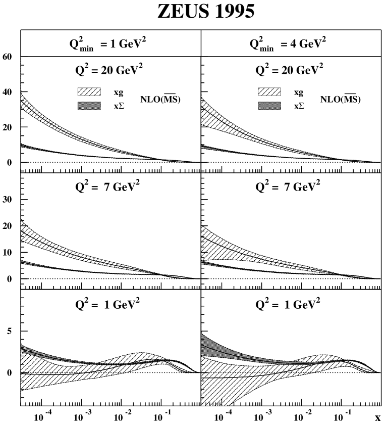
Figure 12: The quark singlet momentum distribution, $x\Sigma$ (shaded), and the gluon momentum distribution, $xg(x)$ (hatched), as functions of $x$ at fixed values of $Q^{2}=1$, 7 and 20 GeV² from the ZEUS QCD fit. The error bands correspond to the quadratic sum of all error sources considered for each parton density. The three left-hand plots show the results from the standard fit of Sec. 6 including $F_{2}$ data with $Q^{2}>1\mbox{\hskip 3.00003pt\rm GeV}^{2}$; the three right-hand plots show the corresponding results from the fit described in Sec. 7 for which the data must satisfy $Q^{2}>4\mbox{\hskip 3.00003pt\rm GeV}^{2}$.

The three left-hand plots of Fig. 12 show the distributions for $x\Sigma$ and $xg$ as functions of $x$ for $Q^{2}$ at 1, 7 and $20\mbox{\hskip 3.00003pt\rm GeV}^{2}$. The error bands shown correspond to the quadratic sum of all error sources. It can be seen that even at the smallest $Q^{2}$ the quark singlet distribution, $x\Sigma$, is rising at small $x$ whereas the gluon distribution, xg, has become almost flat, indeed compatible with zero. This behaviour has also been found by others, for instance Martin et al. (MRST) [46] in their recent global determination of parton densities. At $Q^{2}=1$ GeV² the gluon distribution is poorly determined and can, within errors, be negative at low $x$. In the simplest form of the parton model (and leading order QCD) this would clearly be unphysical and while it is known that at NLO in the $\overline{\rm{MS}}$  scheme a positive parton density will remain positive for forward evolution in $Q^{2}$ there is no such constraint for backwards evolution [61]. A negative gluon distribution is therefore not necessarily in contradiction with perturbative NLO QCD provided cross-sections or structure functions calculated from the parton distributions are positive for all $x$ and $Q^{2}$ in the fitted kinematic domain. We have verified that this is the case for $F_{2}^{c}$ and the longitudinal structure function $F_{L}$.

7 The transition region and NLO QCD

7.1 The NLO QCD fit at low $Q^{2}$

It is now widely observed that NLO DGLAP QCD fits give good descriptions of $F_{2}$ data down to $Q^{2}$ values in the range $1-2\mbox{\hskip 3.00003pt\rm GeV}^{2}$. For such fits to be valid one assumes:

1. the validity of the DGLAP QCD formalism;

2. NLO is sufficient even though $\alpha_{S}$ is becoming large (e.g. for this analysis $\alpha_{S}=0.46$ at $1\mbox{\hskip 3.00003pt\rm GeV}^{2}$ );

3. that no higher twist terms, shadowing or other non-perturbative effects contribute to $F_{2}$.

In this paper we have also deliberately made the minimum of assumptions about the low $x$ functional form of the parton distributions at $Q^{2}_{0}$. We require only that they must tend to zero as $x\to 1$ and that the flavour and momentum sum-rules are respected.

To investigate the stability of our results at low $Q^{2}$ we have repeated the full QCD fit and error evaluation procedure on the same data as in Sec. 6 but with the minimum $Q^{2}$ cut ($Q^{2}_{min}$) raised to $4\mbox{\hskip 3.00003pt\rm GeV}^{2}$. The quality of the fit is much as before, $\chi^{2}$ of 1242 for 943 data points and 11 parameters (statistical and systematic errors added in quadrature). The resulting $x\Sigma$ and $xg$ parton distributions are shown in the three right-hand plots of Fig. 12. Qualitatively the features shown by the standard fit (left-hand plots) are unchanged. The rising $x\Sigma$ distribution at low $x$ remains and the sea dominates the gluon at small $x$ and the lowest $Q^{2}$ value. In more detail:

• The parton densities from the central fits with $Q^{2}_{min}=1$ and $4\mbox{\hskip 3.00003pt\rm GeV}^{2}$ are very similar.

• Except at the lowest $Q^{2}$, the precision of the determination of $x\Sigma$ is not much reduced. Even at $Q^{2}=1\mbox{\hskip 3.00003pt\rm GeV}^{2}$, $x\Sigma$ is reasonably well determined for $x>3\times 10^{-4}$, at smaller $x$ values there are insufficient data to constrain the fit.

• At all $Q^{2}$ values shown in the right-hand plots the precision of the determination of $xg$ for $x<10^{-3}$ is worse.

The increase in the error bands for the gluon density when the $Q^{2}_{min}$ cut is increased shows the importance of the SVX95 data at low $x$ and low $Q^{2}$ in determining $xg$ in this region.

To investigate if there is a technical lower limit to the NLO QCD fit (in the sense that the fit fails to converge or gives a very bad $\chi^{2}$), we extend the QCD fit into the region covered by the ZEUS BPC95 data by lowering the $Q^{2}_{min}$ cut to 0.4 GeV². The fit gives an acceptable description of the data with $F_{2}^{c}$ positive and $F_{L}$ (calculated as in [62]) only slightly negative at $x\approx 5\times 10^{-3}$ and $Q^{2}=0.5$ GeV². We therefore conclude that we do not observe a significant breakdown of the NLO DGLAP description in the kinematic range explored. However, we stress that, within the present experimental accuracy, $F_{2}$ data by itself cannot validate the assumptions noted at the beginning of this section and that other information such as precise measurements of $F_{2}^{c}$ in DIS, measurements of other hard processes or more theoretical input is required. 

7.2 $F_{2}$ slopes and models

In order to clarify what we have learned about the transition region from the ZEUS Regge fit and the NLO DGLAP fits we return to the $F_{2}$ slopes.

Fig. 7, showing the ZEUS+E665 $\lambda_{eff}$ data of Sec. 5.1, also shows the calculation from the ZEUSREGGE fit of Sec. 4 and for $Q^{2}>1\mbox{\hskip 3.00003pt\rm GeV}^{2}$ the result from the ZEUSQCD fit of Sec. 6. In the BPC region, the ZEUSREGGE (full line) calculation gives $\lambda_{eff}$ somewhat higher than that given by the original DL Regge fit (dashed line), but it is still below the data. This is largely because the ZEUSREGGE fit includes low $W$ photoproduction data and thus gives a lower $\alpha_{P}$ than the value of $1.141$ from the Regge fit to the extrapolated ZEUS BPC $\sigma_{0}^{\gamma p}$ data alone. At larger $Q^{2}$ values, ZEUSQCD (full line) gives a good account of the trend and normalisation of $\lambda_{eff}$ while GRV94 (dashed line) tends to predict a larger value of $\lambda_{eff}$, which means a steeper rise of $F_{2}$ as $x$ decreases, than that determined from the data.

Fig. 9 shows the ZEUS $dF_{2}/d\ln Q^{2}$ data together with the same two calculations, ZEUSREGGE at very low $x$ and $Q^{2}$ values and ZEUSQCD for $Q^{2}>1\mbox{\hskip 3.00003pt\rm GeV}^{2}$. The ZEUSREGGE points show much the same trend as that of the original DL model. At $Q^{2}$ values between 1 and $5\mbox{\hskip 3.00003pt\rm GeV}^{2}$, the ZEUSQCD points are qualitatively different from those of GRV94. The ZEUSQCD values now follow the ‘turn over’ of the slope data around $x\sim 3\times 10^{-4}$. This has also been found by MRST in [46] where they compare their global fit to $dF_{2}/d\ln Q^{2}$ data from H1, ZEUS and the NMC experiments. The rise in $F_{2}$ at low $x$ and the ‘turn over’ in $dF_{2}/d\ln Q^{2}$ reflect the different behaviours of the gluon and $q\bar{q}$ sea distributions at $Q^{2}\sim 1\mbox{\hskip 3.00003pt\rm GeV}^{2}$. For very small $x$ the sea continues to rise ($\delta_{s}<0$ in the notation of Eq. (6)) whereas the gluon rises significantly less steeply or even tends to zero ($\delta_{g}\geq 0$).

In contrast, for the GRV94 parton densities GRV assume that at their low starting scale of $0.34\mbox{\hskip 3.00003pt\rm GeV}^{2}$ both the gluon and the sea distributions are non-singular. All the rise of $F_{2}$ at low $x$ for $Q^{2}>1\mbox{\hskip 3.00003pt\rm GeV}^{2}$ is then generated through the DGLAP evolution equations. In a recent paper GRV [64] have revisited their ‘dynamical parton model’ in the light of the HERA 1994 data and have produced a new set of parton distributions – GRV98. They find that they can correct most of the discrepancies between GRV94 and the HERA data by a slight increase in the starting scale from $0.34$ to $0.4\mbox{\hskip 3.00003pt\rm GeV}^{2}$ and by using a lower value of $\alpha_{S}(M^{2}_{Z})=0.114$ rather than the value of $0.118$ used in the ZEUS NLO QCD fit. They acknowledge that if they use a larger value of $\alpha_{S}$ then their starting scale has to be increased to around $1\mbox{\hskip 3.00003pt\rm GeV}^{2}$ and they have to accept a rising $q\bar{q}$ sea distribution at the starting scale.

8 Summary and conclusions

In this paper we have presented the measurement by ZEUS of $F_{2}$ in the $Q^{2}$ region $0.6-17\mbox{\hskip 3.00003pt\rm GeV}^{2}$ (SVX95), which fills the gap between the very low $Q^{2}$ BPC95 data ($0.11-0.65\mbox{\hskip 3.00003pt\rm GeV}^{2}$) and the large 1994 data sample ($3.5-5000\mbox{\hskip 3.00003pt\rm GeV}^{2}$). We have shown that the BPC data may be described successfully by non-perturbative approaches: a simple generalised vector dominance model for the $Q^{2}$ dependence and a two component Regge model for the $W^{2}$ dependence. For $Q^{2}\geq 0.9\mbox{\hskip 3.00003pt\rm GeV}^{2}$ these approaches fail to describe the dominant feature of the data, which is the rapid rise of $F_{2}$ at small $x$.

We have studied the transition region by fitting $F_{2}=Ax^{-\lambda_{eff}}$ using ZEUS and E665 data with $x<0.01$ in the $Q^{2}$ range $0.15-250\mbox{\hskip 3.00003pt\rm GeV}^{2}$. For $Q^{2}>0.9\mbox{\hskip 3.00003pt\rm GeV}^{2}$ the data are not compatible with the $Q^{2}$ independence of $\lambda_{eff}$, as expected for a dominant Pomeron term in conventional Regge theory, but are well described by the ZEUS NLO QCD fit.

The slope $dF_{2}/d\ln Q^{2}$ has been calculated from ZEUS $F_{2}$ data in the range $2\times 10^{-6}<x<0.2$. Assuming pQCD, $F_{2}$ at low $x$ is largely determined by the $q\bar{q}$ sea density whereas $dF_{2}/d\ln Q^{2}$ is given by the gluon density. As $x$ decreases the slope values increase until at $x\approx 3\times 10^{-4}$ there is a turn over and for smaller $x$ values the slope values decrease.

To study the behaviour of the parton densities in more detail we have performed a NLO DGLAP QCD fit to ZEUS and fixed target data with $Q^{2}>1\mbox{\hskip 3.00003pt\rm GeV}^{2}$ and $3\times 10^{-5}<x<0.7$. A good description of the $F_{2}$ data over the whole range of $Q^{2}$ from 1 to $5000\mbox{\hskip 3.00003pt\rm GeV}^{2}$ is obtained. Around the lower $Q^{2}$ limit of the fit we find that the $q\bar{q}$ sea distribution is still rising at small $x$, whereas the gluon distribution is strongly suppressed. These findings are incompatible with the hypothesis that the rapid rise in $F_{2}$ is driven by the rapid increase in gluon density at small $x$ from parton splitting alone. These features remain true if the lowest $Q^{2}$ for which data is included in the fit is raised from 1 to $4\mbox{\hskip 3.00003pt\rm GeV}^{2}$.

From the ZEUS QCD fit we also obtain a much improved determination of the gluon momentum density compared to the previous determination by ZEUS [5]. Full account has been taken of correlated experimental systematic errors and the uncertainty in the form of the input gluon distribution function has also been estimated. At $Q^{2}=20\mbox{\hskip 3.00003pt\rm GeV}^{2}$ and $x=5\times 10^{-5}$ the total fractional error on the gluon density has been reduced from 40% to 10%.

We have used NLO pQCD and the simplest non-perturbative models to study the transition region in $Q^{2}$. We find, for $Q^{2}\geq 0.9\mbox{\hskip 3.00003pt\rm GeV}^{2}$, that the wholly non-perturbative description fails. Although pQCD may not be valid at such low scales, we have not been able to find a lower limit at which the NLO DGLAP fit breaks down conclusively.

Appendix

The following tables are also available via the ZEUS collaboration home page, http://www-zeus.desy.de/. Fortran routines and data files to calculate the parton distributions from the ZEUS NLO QCD fits are also available from this site.

bin	$x$	$Q^{2}$ ($\mbox{\hskip 3.00003pt\rm GeV}^{2}$)	$F_{2}$	error $stat._{-sys}^{+sys}$	$F_{2}~{}(F_{L}=0)$
1	$1.2\cdot 10^{-5}$	$0.6$	$0.531$	$\pm 0.030_{-0.060}^{+0.037}$	$0.517$
2	$1.9\cdot 10^{-5}$	$0.9$	$0.653$	$\pm 0.030_{-0.053}^{+0.067}$	$0.632$
3	$2.6\cdot 10^{-5}$	$0.9$	$0.655$	$\pm 0.023_{-0.037}^{+0.039}$	$0.644$
4	$3.6\cdot 10^{-5}$	$0.9$	$0.574$	$\pm 0.022_{-0.050}^{+0.034}$	$0.570$
5	$2.8\cdot 10^{-5}$	$1.3$	$0.716$	$\pm 0.029_{-0.065}^{+0.069}$	$0.687$
6	$3.8\cdot 10^{-5}$	$1.3$	$0.717$	$\pm 0.023_{-0.037}^{+0.043}$	$0.703$
7	$5.3\cdot 10^{-5}$	$1.3$	$0.715$	$\pm 0.022_{-0.041}^{+0.036}$	$0.708$
8	$8.0\cdot 10^{-5}$	$1.3$	$0.626$	$\pm 0.017_{-0.031}^{+0.033}$	$0.624$
9	$1.6\cdot 10^{-4}$	$1.3$	$0.559$	$\pm 0.016_{-0.047}^{+0.046}$	$0.558$
10	$3.9\cdot 10^{-5}$	$1.9$	$0.915$	$\pm 0.036_{-0.070}^{+0.071}$	$0.873$
11	$5.3\cdot 10^{-5}$	$1.9$	$0.852$	$\pm 0.028_{-0.051}^{+0.033}$	$0.833$
12	$7.5\cdot 10^{-5}$	$1.9$	$0.742$	$\pm 0.025_{-0.026}^{+0.038}$	$0.734$
13	$1.1\cdot 10^{-4}$	$1.9$	$0.740$	$\pm 0.023_{-0.038}^{+0.035}$	$0.736$
14	$2.2\cdot 10^{-4}$	$1.9$	$0.636$	$\pm 0.019_{-0.057}^{+0.026}$	$0.635$
15	$5.4\cdot 10^{-5}$	$2.5$	$0.964$	$\pm 0.039_{-0.060}^{+0.060}$	$0.916$
16	$7.3\cdot 10^{-5}$	$2.5$	$0.909$	$\pm 0.029_{-0.040}^{+0.044}$	$0.887$
17	$1.0\cdot 10^{-4}$	$2.5$	$0.870$	$\pm 0.027_{-0.044}^{+0.022}$	$0.860$
18	$1.6\cdot 10^{-4}$	$2.5$	$0.771$	$\pm 0.023_{-0.016}^{+0.050}$	$0.767$
19	$3.0\cdot 10^{-4}$	$2.5$	$0.725$	$\pm 0.023_{-0.060}^{+0.029}$	$0.724$
20	$7.3\cdot 10^{-5}$	$3.5$	$1.140$	$\pm 0.050_{-0.057}^{+0.058}$	$1.081$
21	$9.8\cdot 10^{-5}$	$3.5$	$0.995$	$\pm 0.035_{-0.023}^{+0.040}$	$0.970$
22	$1.4\cdot 10^{-4}$	$3.5$	$0.945$	$\pm 0.031_{-0.022}^{+0.034}$	$0.933$
23	$2.1\cdot 10^{-4}$	$3.5$	$0.839$	$\pm 0.026_{-0.028}^{+0.019}$	$0.834$
24	$4.1\cdot 10^{-4}$	$3.5$	$0.663$	$\pm 0.021_{-0.048}^{+0.044}$	$0.661$
25	$1.0\cdot 10^{-4}$	$4.5$	$1.160$	$\pm 0.043_{-0.044}^{+0.040}$	$1.108$
26	$1.7\cdot 10^{-4}$	$4.5$	$1.005$	$\pm 0.031_{-0.037}^{+0.050}$	$0.990$
27	$2.8\cdot 10^{-4}$	$4.5$	$0.912$	$\pm 0.030_{-0.032}^{+0.029}$	$0.907$
28	$5.4\cdot 10^{-4}$	$4.5$	$0.664$	$\pm 0.022_{-0.057}^{+0.055}$	$0.663$
29	$1.4\cdot 10^{-4}$	$6$	$1.305$	$\pm 0.055_{-0.037}^{+0.041}$	$1.247$
30	$2.2\cdot 10^{-4}$	$6$	$1.086$	$\pm 0.039_{-0.046}^{+0.025}$	$1.070$
31	$3.7\cdot 10^{-4}$	$6$	$1.002$	$\pm 0.038_{-0.033}^{+0.027}$	$0.996$
32	$7.1\cdot 10^{-4}$	$6$	$0.753$	$\pm 0.028_{-0.079}^{+0.050}$	$0.751$
33	$1.8\cdot 10^{-4}$	$7.5$	$1.210$	$\pm 0.058_{-0.051}^{+0.037}$	$1.167$
34	$3.6\cdot 10^{-4}$	$7.5$	$0.918$	$\pm 0.036_{-0.023}^{+0.074}$	$0.910$
35	$8.8\cdot 10^{-4}$	$7.5$	$0.810$	$\pm 0.040_{-0.038}^{+0.060}$	$0.808$
36	$2.2\cdot 10^{-4}$	$9$	$1.296$	$\pm 0.061_{-0.074}^{+0.039}$	$1.251$
37	$4.3\cdot 10^{-4}$	$9$	$0.957$	$\pm 0.038_{-0.036}^{+0.028}$	$0.948$
38	$1.1\cdot 10^{-3}$	$9$	$0.818$	$\pm 0.039_{-0.065}^{+0.027}$	$0.816$
39	$2.8\cdot 10^{-4}$	$12$	$1.306$	$\pm 0.057_{-0.038}^{+0.066}$	$1.265$
40	$5.6\cdot 10^{-4}$	$12$	$1.084$	$\pm 0.040_{-0.061}^{+0.043}$	$1.073$
41	$1.4\cdot 10^{-3}$	$12$	$0.956$	$\pm 0.044_{-0.040}^{+0.057}$	$0.954$
42	$3.9\cdot 10^{-4}$	$17$	$1.311$	$\pm 0.057_{-0.055}^{+0.040}$	$1.270$
43	$7.9\cdot 10^{-4}$	$17$	$1.087$	$\pm 0.038_{-0.041}^{+0.051}$	$1.077$
44	$1.9\cdot 10^{-3}$	$17$	$0.931$	$\pm 0.045_{-0.077}^{+0.046}$	$0.927$

Table 1: Values of $x$, $Q^{2}$, $F_{2}$, statistical and systematic errors from the ZEUS 1995 shifted vertex analysis (SVX95).

bin	$W$	$\epsilon$	$\sigma^{\gamma p}_{0}$	stat. err.	sys. err.
	[GeV]		[$\mu$b]	[$\mu$b]	[$\mu$b]
1	104	0.99	156.2	$\pm 5.3$	$\pm 16.1$
2	134	0.98	166.1	$\pm 5.2$	$\pm 11.0$
3	153	0.96	174.7	$\pm 4.9$	$\pm 12.9$
4	173	0.92	175.5	$\pm 5.0$	$\pm 11.7$
5	190	0.88	181.8	$\pm 4.7$	$\pm 12.8$
6	212	0.80	186.8	$\pm 4.8$	$\pm 13.5$
7	233	0.69	192.5	$\pm 4.7$	$\pm 13.3$
8	251	0.55	204.8	$\pm 5.6$	$\pm 17.0$

Table 2: Values of $\sigma^{\gamma p}_{0}$ together with statistical and systematic errors from the GVMD extrapolation, with $\sigma_{L}=0$, of ZEUS BPC95 data. $W$ is the $\gamma^{*}p$ centre-of-mass energy and $\epsilon$ is the polarisation of the virtual photon.

bin	$Q^{2}$ ($\mbox{\hskip 3.00003pt\rm GeV}^{2}$)	$x_{min}$	$x_{max}$	$\langle x\rangle$	$\lambda_{eff}$	error $stat.^{+sys}_{-sys}$
1	0.15	2.4$\cdot 10^{-6}$	4.2$\cdot 10^{-6}$	3.2$\cdot 10^{-6}$	0.134	$\pm 0.077^{+0.189}_{-0.194}$
2	0.2	3.2$\cdot 10^{-6}$	8.5$\cdot 10^{-6}$	5.5$\cdot 10^{-6}$	0.128	$\pm 0.036^{+0.080}_{-0.083}$
3	0.25	4.6$\cdot 10^{-6}$	1.8$\cdot 10^{-3}$	1.3$\cdot 10^{-5}$	0.136	$\pm 0.016^{+0.040}_{-0.044}$
4	0.3	6.7$\cdot 10^{-6}$	2.5$\cdot 10^{-3}$	1.1$\cdot 10^{-4}$	0.110	$\pm 0.007^{+0.017}_{-0.022}$
5	0.4	1.1$\cdot 10^{-5}$	5.2$\cdot 10^{-3}$	6.8$\cdot 10^{-4}$	0.115	$\pm 0.005^{+0.015}_{-0.019}$
6	0.5	2.1$\cdot 10^{-5}$	4.6$\cdot 10^{-5}$	2.9$\cdot 10^{-5}$	0.193	$\pm 0.050^{+0.100}_{-0.097}$
7	0.65	1.2$\cdot 10^{-5}$	5.2$\cdot 10^{-3}$	1.8$\cdot 10^{-3}$	0.114	$\pm 0.007^{+0.016}_{-0.019}$
8	0.9	1.9$\cdot 10^{-5}$	8.9$\cdot 10^{-3}$	3.8$\cdot 10^{-3}$	0.147	$\pm 0.005^{+0.013}_{-0.014}$
9	1.3	2.8$\cdot 10^{-5}$	8.9$\cdot 10^{-3}$	2.4$\cdot 10^{-3}$	0.152	$\pm 0.006^{+0.014}_{-0.014}$
10	1.9	3.9$\cdot 10^{-5}$	8.9$\cdot 10^{-3}$	1.8$\cdot 10^{-3}$	0.160	$\pm 0.008^{+0.014}_{-0.013}$
11	2.5	5.4$\cdot 10^{-5}$	8.9$\cdot 10^{-3}$	1.3$\cdot 10^{-3}$	0.179	$\pm 0.010^{+0.016}_{-0.014}$
12	3.5	6.3$\cdot 10^{-5}$	8.9$\cdot 10^{-3}$	6.1$\cdot 10^{-4}$	0.178	$\pm 0.012^{+0.022}_{-0.018}$
13	4.5	1.0$\cdot 10^{-4}$	5.4$\cdot 10^{-4}$	2.0$\cdot 10^{-4}$	0.261	$\pm 0.020^{+0.042}_{-0.041}$
14	6.5	1.0$\cdot 10^{-4}$	4.0$\cdot 10^{-3}$	7.9$\cdot 10^{-4}$	0.192	$\pm 0.005^{+0.016}_{-0.012}$
15	8.5	1.6$\cdot 10^{-4}$	1.6$\cdot 10^{-3}$	6.7$\cdot 10^{-4}$	0.261	$\pm 0.012^{+0.016}_{-0.020}$
16	10	1.6$\cdot 10^{-4}$	6.3$\cdot 10^{-3}$	1.6$\cdot 10^{-3}$	0.226	$\pm 0.007^{+0.015}_{-0.014}$
17	12	2.5$\cdot 10^{-4}$	2.5$\cdot 10^{-3}$	9.7$\cdot 10^{-4}$	0.250	$\pm 0.014^{+0.018}_{-0.020}$
18	15	2.5$\cdot 10^{-4}$	6.3$\cdot 10^{-3}$	1.9$\cdot 10^{-3}$	0.249	$\pm 0.010^{+0.016}_{-0.014}$
19	18	3.9$\cdot 10^{-4}$	6.3$\cdot 10^{-3}$	2.1$\cdot 10^{-3}$	0.274	$\pm 0.010^{+0.014}_{-0.013}$
20	22	4.0$\cdot 10^{-4}$	1.0$\cdot 10^{-2}$	3.4$\cdot 10^{-3}$	0.273	$\pm 0.010^{+0.017}_{-0.014}$
21	27	6.3$\cdot 10^{-4}$	6.3$\cdot 10^{-3}$	2.7$\cdot 10^{-3}$	0.332	$\pm 0.015^{+0.017}_{-0.014}$
22	35	6.3$\cdot 10^{-4}$	1.0$\cdot 10^{-2}$	3.7$\cdot 10^{-3}$	0.308	$\pm 0.016^{+0.013}_{-0.019}$
23	45	1.0$\cdot 10^{-3}$	1.0$\cdot 10^{-2}$	3.7$\cdot 10^{-3}$	0.289	$\pm 0.020^{+0.022}_{-0.017}$
24	60	1.0$\cdot 10^{-3}$	1.0$\cdot 10^{-2}$	4.7$\cdot 10^{-3}$	0.342	$\pm 0.021^{+0.009}_{-0.017}$
25	70	1.6$\cdot 10^{-3}$	1.0$\cdot 10^{-2}$	4.8$\cdot 10^{-3}$	0.306	$\pm 0.032^{+0.018}_{-0.023}$
26	90	1.6$\cdot 10^{-3}$	1.0$\cdot 10^{-2}$	5.3$\cdot 10^{-3}$	0.273	$\pm 0.040^{+0.046}_{-0.027}$
27	120	2.5$\cdot 10^{-3}$	1.0$\cdot 10^{-2}$	6.2$\cdot 10^{-3}$	0.380	$\pm 0.059^{+0.001}_{-0.002}$
28	150	2.5$\cdot 10^{-3}$	1.0$\cdot 10^{-2}$	6.3$\cdot 10^{-3}$	0.258	$\pm 0.079^{+0.004}_{-0.004}$
29	200	4.0$\cdot 10^{-3}$	1.0$\cdot 10^{-2}$	7.0$\cdot 10^{-3}$	0.250	$\pm 0.126^{+0.009}_{-0.003}$
30	250	4.0$\cdot 10^{-3}$	1.0$\cdot 10^{-2}$	7.9$\cdot 10^{-3}$	0.452	$\pm 0.184^{+0.008}_{-0.000}$

Table 3: Values of the slope $\lambda_{eff}=d\ln F_{2}/d\ln(1/x)$ and their errors, calculated from fitting $F_{2}=Ax^{-\lambda_{eff}}$ at fixed $Q^{2}$ to ZEUS and E665 data with $x<0.01$. The columns labelled $x_{min},x_{max}$ and $\langle x\rangle$ give the minimum, maximum and average values of $x$ in a bin. $\langle x\rangle$ is calculated as described in Sec. 5.1 of the text.

bin	$x$	$Q^{2}_{min}$ ($\mbox{\hskip 3.00003pt\rm GeV}^{2}$)	$Q^{2}_{max}$	$\langle Q^{2}\rangle$	$dF_{2}/d\ln Q^{2}$	error $stat.^{+sys}_{-sys}$
1	2.1$\cdot 10^{-6}$	0.11	0.15	0.12	0.135	$\pm 0.029^{+0.030}_{-0.029}$
2	3.1$\cdot 10^{-6}$	0.15	0.2	0.16	0.198	$\pm 0.028^{+0.033}_{-0.033}$
3	4.6$\cdot 10^{-6}$	0.15	0.25	0.2	0.174	$\pm 0.017^{+0.047}_{-0.047}$
4	7.3$\cdot 10^{-6}$	0.2	0.3	0.23	0.191	$\pm 0.019^{+0.040}_{-0.040}$
5	1.2$\cdot 10^{-5}$	0.25	0.6	0.29	0.265	$\pm 0.017^{+0.020}_{-0.023}$
6	2.0$\cdot 10^{-5}$	0.3	0.9	0.37	0.297	$\pm 0.018^{+0.026}_{-0.022}$
7	3.3$\cdot 10^{-5}$	0.3	1.9	0.52	0.312	$\pm 0.009^{+0.032}_{-0.031}$
8	6.3$\cdot 10^{-5}$	0.5	3.5	1.1	0.365	$\pm 0.010^{+0.032}_{-0.032}$
9	1.0$\cdot 10^{-4}$	1.3	6.5	2.5	0.379	$\pm 0.018^{+0.049}_{-0.043}$
10	1.6$\cdot 10^{-4}$	1.3	10	3.8	0.387	$\pm 0.013^{+0.038}_{-0.038}$
11	2.5$\cdot 10^{-4}$	1.9	15	5.2	0.368	$\pm 0.013^{+0.043}_{-0.029}$
12	4.0$\cdot 10^{-4}$	3.5	22	8.8	0.429	$\pm 0.018^{+0.044}_{-0.035}$
13	6.3$\cdot 10^{-4}$	4.5	35	10	0.404	$\pm 0.015^{+0.040}_{-0.035}$
14	1.0$\cdot 10^{-3}$	6.5	60	13	0.315	$\pm 0.014^{+0.018}_{-0.020}$
15	1.6$\cdot 10^{-3}$	6.5	90	14	0.262	$\pm 0.012^{+0.015}_{-0.012}$
16	2.5$\cdot 10^{-3}$	6.5	150	19	0.227	$\pm 0.009^{+0.011}_{-0.017}$
17	4.0$\cdot 10^{-3}$	6.5	250	26	0.139	$\pm 0.008^{+0.019}_{-0.007}$
18	6.3$\cdot 10^{-3}$	10	450	24	0.150	$\pm 0.008^{+0.015}_{-0.008}$
19	1.0$\cdot 10^{-2}$	22	800	56	0.119	$\pm 0.012^{+0.022}_{-0.018}$
20	1.6$\cdot 10^{-2}$	6.5	1200	19	0.059	$\pm 0.005^{+0.011}_{-0.022}$
21	2.5$\cdot 10^{-2}$	22	1500	45	0.061	$\pm 0.008^{+0.020}_{-0.010}$
22	4.0$\cdot 10^{-2}$	6.5	2000	167	0.037	$\pm 0.007^{+0.019}_{-0.045}$
23	8.1$\cdot 10^{-2}$	10	5000	156	0.018	$\pm 0.004^{+0.016}_{-0.022}$
24	0.2	90	5000	388	0.008	$\pm 0.010^{+0.005}_{-0.010}$

Table 4: Values of the slope $dF_{2}/d\ln Q^{2}$ and their errors calculated from fitting ZEUS $F_{2}$ data to the form $a+b\ln Q^{2}$. The columns labelled $Q^{2}_{min},Q^{2}_{max}$ and $\langle Q^{2}\rangle$ give the minimum, maximum and average values of $Q^{2}$ in a bin. $\langle Q^{2}\rangle$ is calculated as described in Sec. 5.2 of the text.

Parameter	$xg(x)$	$xS(x)$	$x\Delta_{ud}(x)$
$A$	1.77	0.520	6.07
$\delta$	-0.225	-0.241	1.27
$\eta$	9.07	8.60	3.68
$\varepsilon$		0.290
$\gamma$	3.00	8.27

Table 5: Values for the parameters of the nominal ZEUS NLO QCD fit (ZEUSQCD) at the starting scale $Q_{0}^{2}=7\mbox{\hskip 3.00003pt\rm GeV}^{2}$. The parameters are defined in Eq. (6) of the text.

Figure 2: Distributions from the SVX95 analysis showing the comparison between data and simulation: (a) $\delta$ or $E-P_{Z}$ as defined in Sec. 3.3; (b) the $Z$-position of the primary vertex; (c) the positron scattering angle $\theta_{e}$; (d) the energy, $E^{\prime}_{e}$, of the scattered positron; (e) $\log_{10}Q^{2}$; (f) $\log_{10}y$. In all cases the data are represented by filled circles, the simulation by the open histograms and the photoproduction background (calculated from the MC described in Sec. 3.1) by the filled triangles. Both MC calculations are normalised to the luminosity of the data.

Figure 3: The ZEUS SVX95 $F_{2}$ data as a function of $x$ for different $Q^{2}$ bins together with previous ZEUS data (ZEUS 1994 [4], ZEUS BPC 1995 [2]), data from H1 SVX95 [31] and fixed target data (E665 [32]). Error bars correspond to the statistical and systematic errors added in quadrature. The overall normalisation errors are not shown. The curves shown are (dotted) the Donnachie-Landshoff Regge model [22] and (full) the ZEUS NLO QCD fit.

Figure 5: Upper plot. ZEUS BPC measurements of the total cross-section $\sigma_{T}+\epsilon\sigma_{L}$ in bins of $W$ as a function of $Q^{2}$ and the GVMD fit to the data. Lower plot. $\sigma_{\rm tot}^{\gamma p}$ as a function of $W^{2}$. The ZEUS BPC95 points are those from the GVMD extrapolation ($\sigma_{0}^{\gamma p}$). Also shown are direct measurements of the total photoproduction cross-section from H1, ZEUS and earlier experiments at low energies. The curves show Regge fits: the original DL fit [22] to the low $W$ data (dotted); the Pomeron only fit to the BPC $\sigma_{0}^{\gamma p}$ data (dashed) and the Pomeron+Reggeon fit to the low $W$ and BPC $\sigma_{0}^{\gamma p}$ data (full).

Figure 7: $\lambda_{eff}=d\ln F_{2}/d\ln(1/x)$ as a function of $Q^{2}$ calculated by fitting $F_{2}=Ax^{-\lambda_{eff}}$ to ZEUS and E665 data with $x<0.01$. The inner error bar shows the statistical error and the outer the total statistical and systematic error added in quadrature. $\langle x\rangle$ is calculated as described in Sec. 5.1. The DL and GRV94 calculations, shown as points linked by dashed lines, are from the Donnachie-Landshoff Regge fit [22] and the GRV94 NLO QCD fit [8], respectively. The ZEUSREGGE and ZEUSQCD calculations, shown as points linked by full lines, are from the ZEUS Regge and NLO QCD fits described in Secs 4 and 6 of the text respectively. In all cases the points are obtained using the same weighted range of $x$ as for the experimental data.

Figure 8: $F_{2}$ as a function of $Q^{2}$ in bins of $x$ from the ZEUS data sets BPC95, SVX95, ZEUS94. The linear fits $F_{2}=a+b\ln Q^{2}$ are also shown. The values of $\langle Q^{2}\rangle$ given in the plots are calculated as described in Sec. 5.2.

Figure 9: $dF_{2}/d\ln Q^{2}$ as a function of $x$ calculated by fitting ZEUS $F_{2}$ data in bins of $x$ to the form $a+b\ln Q^{2}$. The inner error bar shows the statistical error and the outer the total statistical and systematic error added in quadrature. $\langle Q^{2}\rangle$ is calculated as described in Sec. 5.2. The DL and GRV94 calculations, shown as points linked by dashed lines, are from the Donnachie-Landshoff Regge fit [22] and the GRV94 NLO QCD fit [8], respectively. The ZEUSREGGE and ZEUSQCD calculations, shown as points linked by full lines, are from the ZEUS Regge and NLO QCD fits described in Secs 4 and 6 of the text respectively. In all cases the points are obtained using the same weighted range of $Q^{2}$ as for the experimental data.

Figure 10: The proton structure function $F_{2}$ versus $Q^{2}$ at fixed values of $x$. Data are from the ZEUS94 and SVX95 analyses and from the NMC and BCDMS fixed target experiments. The solid lines correspond to the QCD fit described in the text. For clarity an amount $C_{i}=13.6-0.6i$ is added to $F_{2}$ where $i=1$ (18) for the lowest (highest) $x$ value.

References

-
[1]
ZEUS Collaboration, M. Derrick et al., Phys. Lett. B316
(1993) 412; Z. Phys. C65 (1995) 379; ibid C69 (1996) 607;
ibid C72 (1996) 399.
H1 Collaboration, I. Abt et al., Nucl. Phys. B407 (1993) 515; T. Ahmed et al., Nucl. Phys. B439 (1995) 471; H. Aid et al., Nucl. Phys. B470 (1996) 3. - [2] ZEUS Collaboration, J. Breitweg et al., Phys. Lett. B407 (1997) 432..
- [3] ZEUS Collaboration, M. Derrick et al., Z.Phys. C69 (1996) 607.
- [4] ZEUS Collaboration, M. Derrick et al., Z.Phys. C72 (1996) 399.
- [5] ZEUS Collaboration, M. Derrick et al., Phys. Lett. B345 (1995) 576.
-
[6]
G. Parisi, Proc 11th Recontre de Morionde (1976);
G. Altarelli & G. Parisi, Nucl. Phys. B126 (1977) 298;
V. Gribov & L. Lipatov, Sov. Jour. Nucl. Phys. 15 (1972) 438;
L. Lipatov, Sov. Jour. Nucl. Phys. 20 (1975) 94;
Y. Dokshitzer, Sov. Phys. JETP 46 (1977) 641; - [7] M. Glück, E. Reya & A. Vogt, Z.Phys. C48 (1990) 471; C53 (1992) 127.
- [8] M. Glück, E. Reya & A. Vogt, Z.Phys. C67 (1995) 433.
-
[9]
Y. Balitzki & L. Lipatov, Sov. Jour. Nucl. Phys. 28 (1978) 822;
E. Kuraev, L. Lipatov & V. Fadin, Sov. Phys. JETP 45 (1977) 199. -
[10]
V.S. Fadin & L.N. Lipatov, hep-ph/9802290;
M. Ciafaloni & G. Camici, hep-ph/9803389. -
[11]
D.A. Ross, SHEP-98/06 hep-ph/9804332;
Y.V. Kovchegov & A.H. Mueller, CU-TP-889 hep-ph/9805208;
E.M. Levin, TAUP 2501-98 hep-ph/9806228;
J. Blümlein et al., DESY 98-036, WUE-ITP-98-017, hep-ph/9806368. -
[12]
Proc. of the Int’l Workshop on DIS, Rome 1996,
eds A. Negri & G. D’Agostini;
Proc. of the Int’l Workshop on DIS, Chicago 1997, http://www.hep.anl.gov/dis97/;
Proc. of the Int’l Workshop on DIS, Brussels 1998, http://asrv1.iihe.ac.be/dis98/.
- [13] A.M. Cooper-Sarkar, R. Devenish & A. De Roeck, Int. J. Mod. Phys. A13 (1998) 3385.
-
[14]
B.L. Ioffe, Phys. Lett. 40 (1969) 123;
B.L. Ioffe, V.A. Khoze & L.N. Lipatov, Hard Processes, North Holland (1984) 185. - [15] J.J. Sakurai, Ann. Phys. 11 (1960) 1.
- [16] T. Bauer et al., Rev.Mod.Phys. 50 (1978) 261.
- [17] J.J. Sakurai & D. Schildknecht, Phys. Lett. B40 (1972) 121.
- [18] D. Schildknecht & H. Spiesberger, BI-TP 97/25 (1997).
- [19] P. Collins, An Introduction to Regge Theory and High Energy Physics, Cambridge University Press 1977.
- [20] E.M. Levin, Lectures on Regge theory, DESY 97-213.
- [21] A. Donnachie & P. Landshoff, Phys. Lett. B296 (1992) 227.
- [22] A. Donnachie & P. Landshoff, Z. Phys. C61 (1994) 139.
- [23] B. Badelek & J. Kwiecinski, Rev. Mod. Phys. 68 (1996) 445.
- [24] A. Levy, Lectures on low Physics, DESY 97-013.
- [25] H. Spiesberger, K. Charchula & G.A. Schuler , DJANGO6.1.
- [26] K. Kwiatkowski, H. Spiesberger & H.-J. Möhring, Proceedings of the Workshop ‘Physics at HERA’ vol. 3 DESY (1992) 1294.
-
[27]
L. Lönnblad, Comp. Phys. Comm. 71 (1992) 15;
L. Lönnblad, Z. Phys. C65 (1995) 285. -
[28]
H.-U. Bengtsson & T. Sjöstrand,
Comp. Phys. Comm. 46 (1987) 43;
T. Sjöstrand, CERN TH-7112-93 (1994) - [29] H. Abramowicz et al. , Phys. Lett. B269 (1991) 465.
- [30] B. Badelek, J. Kwiecinski & A. Stasto, Z. Phys. C74 (1997) 297.
- [31] H1 collaboration, I. Abt et al., Nucl. Phys. B497 (1997) 3.
- [32] E665 Collaboration, M.R. Adams et al., Phys.Rev.D54 (1996) 3006.
-
[33]
D.O. Caldwell et al., Phys.Rev.Lett. 40 (1978) 1222;
S.I. Alekhin et al., CERN–HERA 87–01 (1987). -
[34]
ZEUS Collaboration, M. Derrick et al., Z. Phys. C63 (1994) 391;
H1 Collaboration, A. Aid et al., Z. Phys. C69 (1995) 27. - [35] ZEUS Collaboration, paper No. 792 submitted to ICHEP98 Vancouver, July 1998.
-
[36]
B. Surrow, Ph.D. Thesis, Univ. Hamburg 1998, DESY-THESIS-1998-004;
J.R. Tickner, D.Phil. Thesis, Univ. Oxford 1997, RAL-TH-97-018. - [37] Regge fits by Donnachie & Landshoff quoted by the Particle Data Group, Phys. Rev. D54 (1996) 191.
- [38] J. Cudell et al., hep-ph/9701312 (1997).
- [39] H. Abramowicz & A. Levy, DESY 97-251.
- [40] H. Navelet, R. Peschanski & S. Wallon, Mod. Phys. Lett A36 (1994) 3393.
- [41] H. Navelet et al., Phys. Lett. B385 (1996) 357.
- [42] H1 Collab., S. Aid et al., Nucl. Phys. B470 (1996) 3.
- [43] K. Prytz, Phys. Lett. B311 (1993) 286; ibid B332 (1994) 393.
- [44] J. Bartels, K. Charchula & J. Feltesse, Proceedings of the workshop ‘Physics at HERA’ DESY 1991, Eds W. Buchmüller & G. Ingelman, p193.
- [45] A. Caldwell, Invited talk at the DESY Theory Workshop on ‘Recent Developments in QCD’, October 1997 (unpublished).
- [46] A.D. Martin et al., Eur. Phys. J. C4 (1998) 463.
- [47] NMC, M. Arneodo et al., Nucl. Phys. B483 (1997) 3.
- [48] BCDMS, A.C. Benvenuti et al., Phys. Lett. B223 (1989) 485 & Phys. Lett. B237 (1990) 592.
- [49] H. Georgi & D. Politzer, Phys. Rev. D14 (1976) 1829.
- [50] M. Virchaux & A. Milsztajn, Phys. Lett. B274 (1992) 221.
- [51] A. Bodek & J.L. Ritchie, Phys. Rev. D23 (1981) 1070.
- [52] G. Gurci, W. Furmanski & R. Petronzio, Nucl. Phys. B175 (1980) 27; W. Furmanski & R. Petronzio, Phys. Lett. 97B (1980) 437 & Z. Phys. C11 (1982) 293.
- [53] S. Riemersma et al., Phys. Lett. B347 (1995) 143 and references therein.
- [54] A.D. Martin, R.G. Roberts & W.J. Stirling, Phys. Lett. B387 (1996) 419.
- [55] Particle Data Group, R.M. Barnett et al., Phys. Rev. D54 (1996) 1.
- [56] M. Botje, QCDNUM version 16.11 (unpublished).
- [57] F. James, Minuit Version 94.1, CERN Program Library Long Writeup D506.
- [58] ZEUS Collaboration, J. Breitweg et al., Phys. Lett. B407 (1997) 402.
- [59] C. Pascaud & F. Zomer, preprint LAL 95-05.
- [60] M. Abramowitz & I.A. Stegun, Handbook of Mathematical Functions, Dover Publications, Inc. (1972).
- [61] W.J. Stirling, private communication.
- [62] G. Altarelli & G. Martinelli, Phys. Lett. B76 (1978) 89.
- [63] C. Lopez, F. Barreiro & F.J. Yndurain, Z. Phys. C72 (1996) 561; F. Barreiro, Proc. ICHEP96 Warsaw, eds Z. Ajduk & A.K. Wroblewski, World Sci. (1997) p653.
- [64] M. Glück, E. Reya & A. Vogt, hep-ph/9806404.