Tests of the JETSET Bose-Einstein correlation model in the $e^{+}e^{-}$ annihilation process

Abstract

Studies of implementation of the simulation of the Bose-Einstein correlation effects in the JETSET particle generator are performed. Analysis of dependance of the one-dimensional correlation function parameters on the presumed boson source size reveals appearance of the effective new length scale, which limits applicability of the simple momentum-shifting mechanism, employed by JETSET to simulate the Bose-Einstein correlation. Two- and three-dimensional correlation functions are analysed as well and compared to the DELPHI data.

1 Introduction

Recent interest in profound studies of the Bose-Einstein correlations (BEC in what follows) was sparked by reports on possible influence of this phenomenon on the measured value of the $W$ boson mass in $e^{+}e^{-}$ annihilation [1, 2]. Estimations of the strength of this influence were done using the Monte Carlo particle generator JETSET [3], which includes a phenomenological model for two-particle BEC simulation. JETSET (together with PYTHIA [3]) is so far the only $e^{+}e^{-}$ annihilation event generator which accounts for BEC. It is known to reproduce well majority of experimental data, including some basic features connected to BEC. However, more sophisticated studies reveal not only certain discrepancies between experimental and model results, but also self-inconsistencies in the model itself [4, 5]. Therefore, it is of particular importance to establish the extent of applicability of this model and to have a full understanding of its advantages and drawbacks.

This work is devoted to studies of the built-in JETSET algorithm which is used to simulate BEC in hadronic decays of $Z$ boson. The following section describes the physical process and corresponding observables. Overview of the studied model is presented in the next section. The last section contains results and discussion.

2 Scope of the study and definitions

The goal of this analysis is to study methods and consequences of implementing Bose-Einstein correlation models in the JETSET event generator, and to find out eventually how can it affect data analysis. To accomplish this goal, Bose-Einstein correlations between pions produced in hadronic decays of the $Z$ boson are investigated. These decays are generated by the JETSET event generator, which uses the so-called Lund string model to simulate electron-positron annihilation events at a given center of mass energy, in our case $E_{cm}=91.2\ GeV$.

Only the correlations between pairs of particles are studied, whith the two-particle correlation function is defined as

$$C_{2}(p_{1},p_{2})=\frac{P(p_{1},p_{2})}{P(p_{1})P(p_{2})}\ ,$$ (1)

where $p_{1}$ and $p_{2}$ are four-momenta of two particles, $P(p_{1},p_{2})$ – two-particle probability density, and $P(p_{1})$ and $P(p_{2})$ denotes single-particle probability densities.

Defined as above $C_{2}$ is parameterized in terms of the invariant four-momenta difference $Q=\sqrt{(\vec{p}_{1}-\vec{p}_{2})^{2}-(E_{1}-E_{2})^{2}}$ as

$$C_{2}(Q)=N(1+\lambda e^{-R^{2}Q^{2}})\ .$$ (2)

This parameterization is one of the most commonly used [6], with the parameter $R$ giving the width (or source size) and $\lambda$ – the strength of the correlation.

In order to be able to compare our results with experimental data, only charged pions were used in the analysis. Although prompt pions produced in the string decay are the most clean sample, we selected only pions produced in decays of prompt $\rho$ mesons, due to the following advantages :
– high sample uniformity: no admixture of particles which are not subject to Bose-Einstein correlations;
– sufficient average multiplicity of the sample: more pions are produced in decays of $\rho$ mesons then promptly from the string.

Studies were performed not only for the one-dimensional correlation function $C_{2}(Q)$, but also for two- and three-dimensional cases. To facilitate calculations, the Longitudinal Centre-of-Mass System [7, 8] (LCMS) was used to measure four-momentum difference. This is the system in which the sum of the two particles momenta is perpendicular to the jet axis, hence only two-jet $q\overline{q}$ events were generated for further simplicity. In LCMS, $Q$ is resolved into $Q_{long}$, parallel to the jet axis, $Q_{t,out}$, collinear with the pair momentum sum, and complementary $Q_{t,side}$, perpendicular to both $Q_{long}$ and $Q_{t,out}$. It is more convenient in some cases to use only two-dimensional picture with longitudinal $Q_{\parallel}\equiv Q_{long}$ and perpendicular $Q_{\perp}=\sqrt{Q_{t,out}^{2}+Q_{t,side}^{2}}$. Parameterization of $C_{2}$ for these two- and three-dimensional cases was chosen correspondingly as

$$C_{2}(Q_{\perp},Q_{\parallel})=N(1+\lambda e^{-Q^{2}_{\perp}R^{2}_{\perp}-Q^{2}_{\parallel}R^{2}_{\parallel}})\ ,$$ (3)

$$C_{2}(Q_{t,out},Q_{t,side},Q_{long})=N(1+\lambda e^{-Q^{2}_{t,out}R^{2}_{t,out}-Q^{2}_{t,side}R^{2}_{t,side}-Q^{2}_{long}R^{2}_{long}})\ .$$ (4)

In high-energy physics experiments involving detectors, it is difficult to construct the product $P(p_{1})P(p_{2})$ from Eq.(1) due to the phase space limitations. Therefore it is often replaced by $P_{0}(p_{1},p_{2})$, which is equal to $P(p_{1})P(p_{2})$ in a hypothetical case of absence of all the correlations. To make our results comparable with experiment, we must construct a reference sample corresponding to $P_{0}(p_{1},p_{2})$. Therefore, the measured two-particle correlation function is calculated as the double-ratio, using the event mixing technique [8] :

$$r_{BE}(Q)=\frac{N^{\pm\pm}_{BE}(Q)}{N^{\pm\pm}_{BE,mix}(Q)}\ ,\ r_{noBE}(Q)=\frac{N^{\pm\pm}_{noBE}(Q)}{N^{\pm\pm}_{noBE,mix}(Q)}\ ,\ C_{2}(Q)=\frac{r_{BE}(Q)}{r_{noBE}(Q)}$$ (5)

Here $N^{\pm\pm}_{BE}(Q)$ is number of like charged pions as a function of the four-momenta difference $Q$ in presence of Bose-Einstein correlations. Subscript “$BE,mix$” denotes same quantity but with pairs of pions picked from different events. Indices “$noBE$” and “$noBE,mix$” correspond to analogous quantities in absence of BEC (i.e., the simulation of BEC is not included into the event generation).

3 Model description

As it was already mentioned, JETSET is the only particle generator which allows and actually includes an algorithm emulating Bose-Einstein correlations. Recall that BEC is the quantum mechanical phenomenon, which has to appear during the fragmentation stage. However, in the standard implementation of BEC in JETSET, the fragmentation and decays of the short-lived particles like $\rho$ are allowed to proceed independently of the Bose-Einstein effect. The BEC simulation algorithm is applied to the final state particles, for which the four-momenta difference $Q_{i,j}$ is being calculated for each pair of identical bosons $i,j$. A shifted smaller $Q^{\prime}_{i,j}$ is then to be found, such that the ratio $C_{2}(Q)$ of “shifted” to the original $Q$ distribution is given by the requested parameterization (Gaussian or exponential). In our case, the Gaussian parameterization identical to the form (2) was used :

$$C_{2}(Q)=1+\lambda e^{-R_{inp}^{2}Q^{2}}\ ,$$ (6)

where $\lambda$ and $R_{inp}$ are input parameters of the model. The input value of $\lambda$ is often set to 1, as it was done in this analysis too. Values of $R_{inp}$ usually are chosen to fit experimental results.

Further, under assumption of a spherical phase space, $Q^{\prime}$ is the solution of the equation :

$$\int\limits_{0}^{Q_{i,j}}\frac{Q^{2}dQ}{\sqrt{Q^{2}+4m^{2}}}=\int\limits_{0}^{Q^{\prime}_{i,j}}C_{2}(Q)\frac{Q^{2}dQ}{\sqrt{Q^{2}+4m^{2}}}\ .$$ (7)

After applying corresponding four-momentum shift to each pair of considered bosons, all particle momenta are re-weighted to satisfy the energy-momentum conservation. This built-in JETSET algorithm works only in terms of the invariant four-momenta difference $Q$, i.e., it does not distinguish between different $Q$ components. This is yet another ambiguous assumption of the model. Also, it does not include particle correlations of higher orders.

Evidently, this algorithm is absolutely phenomenological and is not based on any fundamental theory. It solely changes the final state particles momenta in order to resemble presence of the Bose-Einstein correlations. Moreover, presumption of the spherical shape for the phase space in Eq.(7) is correct only for the case of very low $Q$ (see the following discussion).

In spite of all the ambiguities, JETSET reproduces fairly well experimental data, such as shift of the $\rho$ mass and observed Bose-Einstein correlations in terms of $Q$. It is widely used to calculate acceptance corrections for detectors and for various estimations, like the $W$ mass shift mentioned in the Introduction. To our mind, this peculiarity is worth investigating, if not in order to get better understanding of the BEC influence in experimental data, then at least in order to establish limits of applicability of such a simulation model.

4 Analysis and discussion

One of the most puzzling inconsistencies in the JETSET simulation of BEC is that the input shape of (6) can not be obtained with the same parameters by fitting the resulting measured $C_{2}(Q)$ with formula (2) (see, for example, article by Fiałkowski and Wit [5]). This is mostly due to the improper phase space approximation in Eq.(7). However, this approximation can still be valid for certain input boson source size $R_{inp}$. To find out whether it is true, we studied $C_{2}(Q)$ for different input values of $R_{inp}$ in formula (6).

Measured as the double-ratio (5) two-particle correlation function generated with different input source size $R_{inp}$ was fitted by the form (2). The $\lambda$ parameter always was reproduced at values close to 1, due to the high purity of the sample. The output source size $R$, however, behaved differently, see Fig. 1 and the corresponding table. Preliminary DELPHI results measured in 1991-1995 on all the charged particles are shown in the same table for comparison.

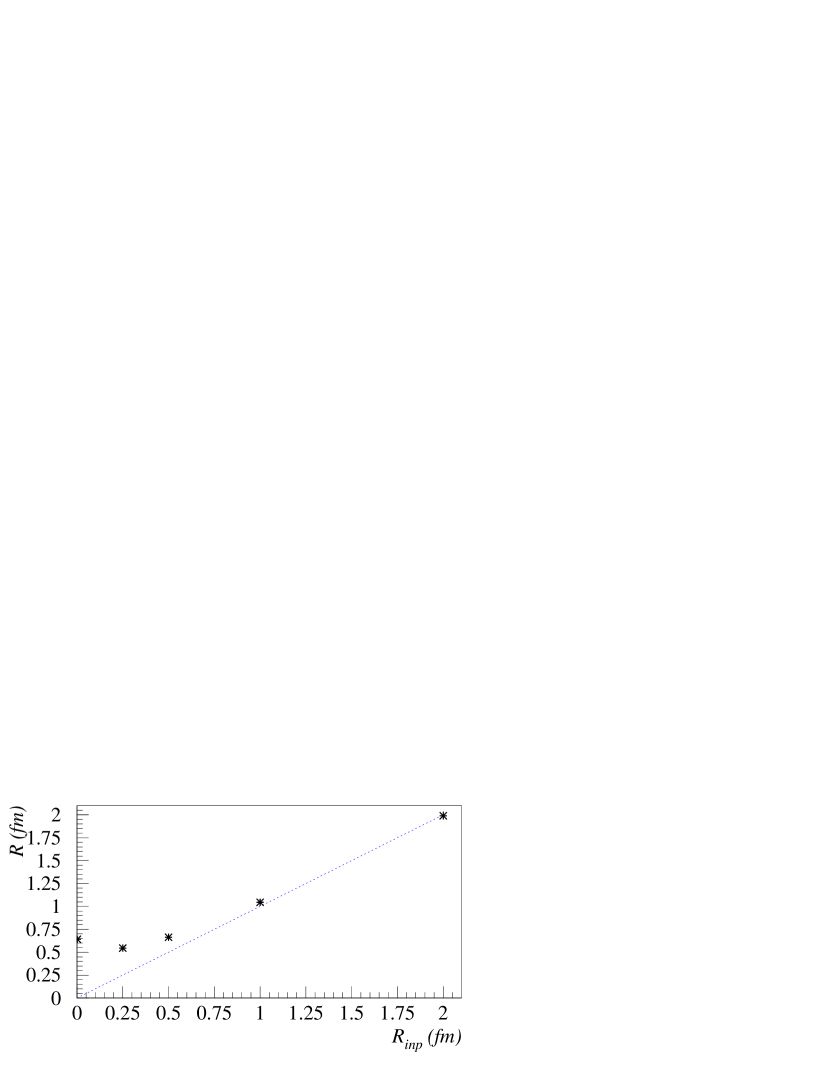
Figure 1: Width $R$ of the measured in JETSET generated events correlation function $C_{2}(Q)$ as a function of the input source radii $R_{inp}$. Line represents the expected dependence.

$R_{inp},fm$	$R,fm$
0.002	$0.640\pm 0.005$
0.250	$0.545\pm 0.006$
0.500	$0.663\pm 0.005$
1.000	$1.046\pm 0.010$
2.000	$1.990\pm 0.042$
DELPHI	$0.489\pm 0.010$

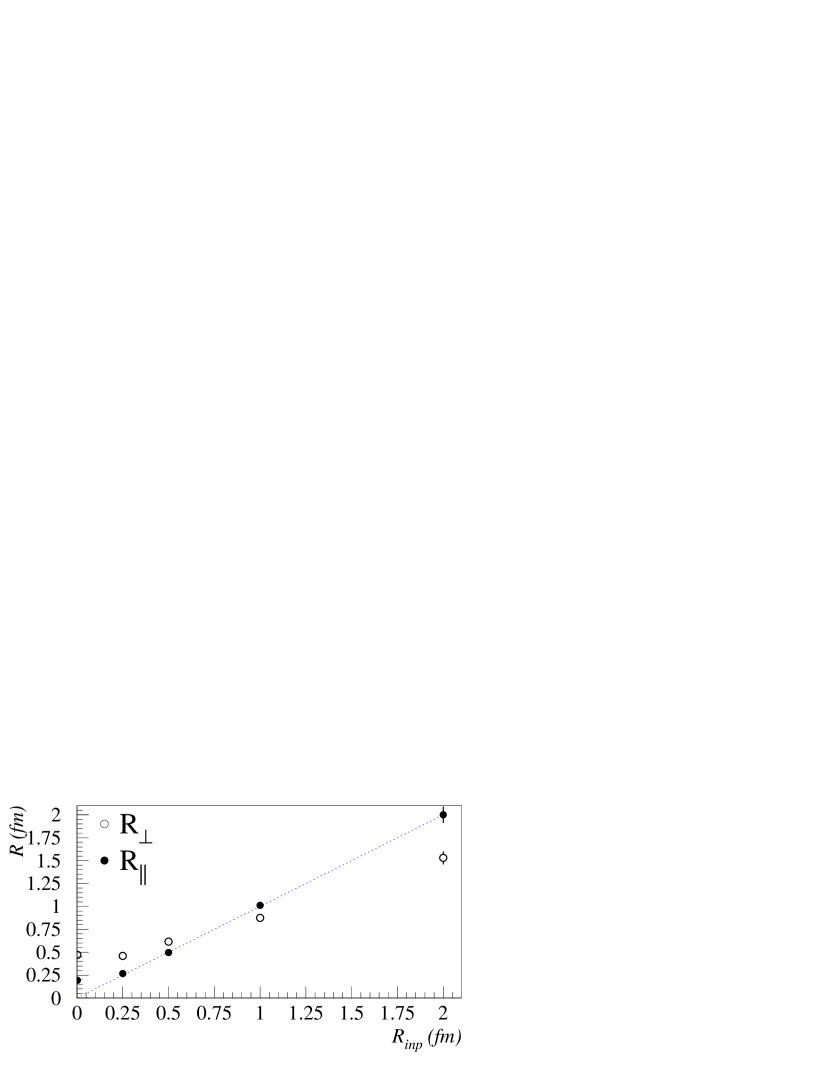
a)

b)

Figure 2: Components of the correlation width as a function of the input source radii $R_{inp}$ : a) $R_{\parallel}$ , $R_{\perp}$ and b) $R_{t,out}$, $R_{t,side}$, $R_{long}$.

$R_{inp},fm$	$R_{\perp},fm$	$R_{\parallel},fm$	$R_{t,out},fm$	$R_{t,side},fm$	$R_{long},fm$
0.002	$0.472\pm 0.002$	$0.193\pm 0.001$	$0.562\pm 0.005$	$0.499\pm 0.004$	$0.193\pm 0.002$
0.250	$0.459\pm 0.003$	$0.266\pm 0.002$	$0.544\pm 0.004$	$0.511\pm 0.004$	$0.307\pm 0.003$
0.500	$0.616\pm 0.005$	$0.497\pm 0.005$	$0.637\pm 0.005$	$0.636\pm 0.005$	$0.549\pm 0.004$
1.000	$0.873\pm 0.015$	$1.013\pm 0.021$	$0.814\pm 0.011$	$0.940\pm 0.012$	$0.986\pm 0.013$
2.000	$1.530\pm 0.070$	$2.000\pm 0.090$	$1.291\pm 0.039$	$1.622\pm 0.051$	$1.835\pm 0.065$
DELPHI	$0.300\pm 0.040$	$0.640\pm 0.020$	$0.364\pm 0.009$	$0.173\pm 0.019$	$0.628\pm 0.008$

It is clearly seen that the measured $R$ does not depend on the input $R_{inp}$ when the latter is below $\approx 0.6\,fm$. For the higher values of $R_{inp}$ JETSET basically reproduces the demanded correlation function.

Knowing that JETSET does not distinguish between components of invariant momentum difference $Q$, we should expect similar behaviour of radius parameters of two- and three-dimensional correlation functions. Parameterization of these functions is performed in a form of a multi-dimensional Gaussians (3) and (4) correspondingly.

As one can see from Fig. 2 and in the corresponding table, transverse radii follow the same pattern as the $R$, while the longitudinal radius tends to reproduce the input value of $R_{inp}$.

All these results show that there is a certain mechanism in the model, which imposes lower limit of around $0.6\,fm$ onto measured $R$ and its transverse components, and almost does not affect the longitudinal radius. The explanation of this phenomenon is illustrated at Fig. 3 for the one-dimensional case. It shows evolution of the $dN/dQ$ distribution with input source radius $R_{inp}$ in comparison with the original non-correlated distribution. It is clearly seen that the expected Bose-Einstein enhancement appears only to the left of the non-correlated distribution peak, $Q<0.3\,GeV$. Since the model conserves multiplicity, and because the assumption of the spherical phase space in Eq.(7) is valid only for this region of the linearly increasing $dN/dQ$, a depletion appears for $Q>0.3\,GeV$, which results in a non-Gaussian output correlation function.

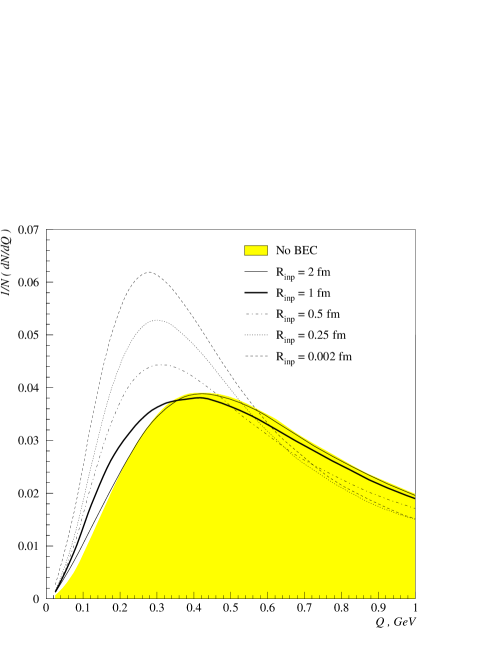
Figure 3: Distribution of $Q$ as a function of the input source radii $R_{inp}$. Shaded area shows this distribution in absence of BEC.

Therefore, the position of the peak in the non-correlated $dN/dQ$ distribution constitutes the limitation of the measured correlation width $R$ and can be interpreted as a new length scale. This conclusion is also valid for transverse correlation radii (see Fig. 4). In the longitudinal direction, $dN/dQ_{\parallel}$ has less rapid falloff and peaks at a very small $Q_{\parallel}$ value due to the LCMS properties, and thus is virtually insensitive to the mentioned length scale.

Figure 4: Two-dimensional distribution $d^{2}N/dQ_{\perp}\,dQ_{\parallel}$ in absence of BEC.

As a result, one should state that the built-in JETSET model for simulating BEC is fully applicable only for sufficiently big sizes of boson source : above $1\,fm$. At the same time, experimental data indicate that this size is around $0.5\,fm$ at the $Z$ peak [9]. This means that, at first, this kind of model has no predictive power. At second, one should be very careful when using JETSET with this model for calculation of detector corrections, because it can not produce an adequate unfolding matrix.

It has to be mentioned that nowadays some other models for simulation of BEC are being developed [10, 11]. They use direct implementation of the Bose-Einstein interference into the string model, being theoretically accurate in this sense. At the moment they take too much computing resources to be used by high-energy physics experiments, but they do have predictive power. One of the most interesting predictions is that the transverse component of the boson source size, $R_{\perp}$, must be significantly smaller then the longitudinal one, $R_{\parallel}$. As one can see, it is being confirmed by the preliminary DELPHI results, but it is not the case for the present JETSET version. This must encourage further works towards developing and implementing advanced models for the BEC simulation in particle generators.

References

References

- [1] L. Lönnblad and T. Sjöstrand, Phys. Lett. B 351, 293 (1995).
- [2] V. Kartvelishvili, R. Kvatadze, R. Møller, “Estimating the effects of Bose-Einstein correlations on the mass measurement at LEP2”, University of Manchester preprint MC-TH-97/04, MAN/HEP/97/1
-
[3]
T. Sjöstrand, Comp. Phys. Comm. 28, 229 (1983);
T. Sjöstrand, Pythia 5.6 and Jetset 7.3, CERN-TH.6488/92 (1992). - [4] S. Haywood, “Where Are We Going With Bose-Einstein – a Mini Review”, RAL Report RAL-94-074
- [5] K. Fiałkowski and R. Wit, Z. Phys. C 74, 145 (1997).
- [6] B. Lörstad, Int. J. Mod. Phys. A4 12, 2861 (1989).
- [7] T. Csörgő and S. Pratt, in “Proceedings of the Workshop on Relativistic Heavy Ion Physics”, KFKI-1991-28/A, p75.
- [8] B. Lörstad, O. Smirnova: “Transverse Mass Dependence of Bose-Einstein Correlation Radii in Annihilation at LEP Energies”: Proceedings of the 7th International Workshop on Multiparticle Production ’Correlations and Fluctuations’, June 30 to July 6, 1996, Nijmegen, The Netherlands.
-
[9]
OPAL Coll., P .D. Acton et al., Phys. Lett. B 267, 143 (1991);
DELPHI Coll., P. Abreu et al., Phys. Lett. B 286, 201 (1992);
ALEPH Coll., D. Decamp et al., Z. Phys. C 54, 75 (1992). -
[10]
B. Andersson and M. Ringnér, Nucl. Phys. B 513, 627 (1998);
B. Andersson and M. Ringnér, Phys. Lett. B 421, 283 (1998). - [11] Ŝ. Todorova-Nová, J. Rames̆, “ Simulation of Bose-Einstein effect using space-time aspects of Lund string fragmentation model”, IReS 97-29, PRA-HEP 97/16.