EUROPEAN LABORATORY FOR PARTICLE PHYSICS

CERN-EP/98-102

June 22, 1998

Measurement of the Strong Coupling Constant α𝐬subscript𝛼𝐬\alpha_{\rm s} and the Vector and Axial-Vector Spectral Functions in Hadronic Tau Decays


The OPAL Collaboration


The spectral functions of the vector current and the axial-vector current have been measured in hadronic τ𝜏\mathrm{\tau} decays using the OPAL detector at LEP. Within the framework of the Operator Product Expansion a simultaneous determination of the strong coupling constant αssubscript𝛼s\alpha_{\rm s}, the non-perturbative operators of dimension 6 and 8 and of the gluon condensate has been performed. Different perturbative descriptions have been compared to the data. The Contour Improved Fixed Order Perturbation Theory gives αs(mτ2)=0.348±0.009exp±0.019theosubscript𝛼ssuperscriptsubscript𝑚𝜏2plus-or-minus0.348subscript0.009expsubscript0.019theo\alpha_{\rm s}(m_{\mathrm{\tau}}^{2})=0.348\pm 0.009_{\rm exp}\pm 0.019_{\rm theo} at the τ𝜏\mathrm{\tau}-mass scale and αs(mZ2)=0.1219±0.0010exp±0.0017theosubscript𝛼ssuperscriptsubscript𝑚Z2plus-or-minus0.1219subscript0.0010expsubscript0.0017theo\alpha_{\rm s}(m_{\mathrm{Z}}^{2})=0.1219\pm 0.0010_{\rm exp}\pm 0.0017_{\rm theo} at the Z0superscriptZ0\mathrm{Z^{0}}-mass scale. The values obtained for αs(mZ2)subscript𝛼ssuperscriptsubscript𝑚Z2\alpha_{\rm s}(m_{\mathrm{Z}}^{2}) using Fixed Order Perturbation Theory or Renormalon Chain Resummation are 2.3%percent2.32.3\,\% and 4.1%percent4.14.1\,\% smaller, respectively. The ‘running’ of the strong coupling between s01.3GeV2similar-to-or-equalssubscript𝑠01.3superscriptGeV2s_{0}\simeq 1.3\,{\rm GeV}^{2} and s0=mτ2subscript𝑠0superscriptsubscript𝑚𝜏2s_{0}=m_{\mathrm{\tau}}^{2} has been tested from direct fits to the integrated differential hadronic decay rate Rτ(s0)subscript𝑅𝜏subscript𝑠0R_{\tau}(s_{0}). A test of the saturation of QCD sum rules at the τ𝜏\mathrm{\tau}-mass scale has been performed.

(Submitted to European Physical Journal C)


The OPAL Collaboration


K. Ackerstaff8, G. Alexander23, J. Allison16, N. Altekamp5, K.J. Anderson9, S. Anderson12, S. Arcelli2, S. Asai24, S.F. Ashby1, D. Axen29, G. Azuelos18,a, A.H. Ball17, E. Barberio8, R.J. Barlow16, R. Bartoldus3, J.R. Batley5, S. Baumann3, J. Bechtluft14, T. Behnke8, K.W. Bell20, G. Bella23, S. Bentvelsen8, S. Bethke14, S. Betts15, O. Biebel14, A. Biguzzi5, S.D. Bird16, V. Blobel27, I.J. Bloodworth1, M. Bobinski10, P. Bock11, J. Böhme14, M. Boutemeur34, S. Braibant8, P. Bright-Thomas1, R.M. Brown20, H.J. Burckhart8, C. Burgard8, R. Bürgin10, P. Capiluppi2, R.K. Carnegie6, A.A. Carter13, J.R. Carter5, C.Y. Chang17, D.G. Charlton1,b, D. Chrisman4, C. Ciocca2, P.E.L. Clarke15, E. Clay15, I. Cohen23, J.E. Conboy15, O.C. Cooke8, C. Couyoumtzelis13, R.L. Coxe9, M. Cuffiani2, S. Dado22, G.M. Dallavalle2, R. Davis30, S. De Jong12, L.A. del Pozo4, A. de Roeck8, K. Desch8, B. Dienes33,d, M.S. Dixit7, M. Doucet18, J. Dubbert34, E. Duchovni26, G. Duckeck34, I.P. Duerdoth16, D. Eatough16, P.G. Estabrooks6, E. Etzion23, H.G. Evans9, F. Fabbri2, A. Fanfani2, M. Fanti2, A.A. Faust30, F. Fiedler27, M. Fierro2, H.M. Fischer3, I. Fleck8, R. Folman26, A. Fürtjes8, D.I. Futyan16, P. Gagnon7, J.W. Gary4, J. Gascon18, S.M. Gascon-Shotkin17, C. Geich-Gimbel3, T. Geralis20, G. Giacomelli2, P. Giacomelli2, V. Gibson5, W.R. Gibson13, D.M. Gingrich30,a, D. Glenzinski9, J. Goldberg22, W. Gorn4, C. Grandi2, E. Gross26, J. Grunhaus23, M. Gruwé27, G.G. Hanson12, M. Hansroul8, M. Hapke13, C.K. Hargrove7, C. Hartmann3, M. Hauschild8, C.M. Hawkes5, R. Hawkings27, R.J. Hemingway6, M. Herndon17, G. Herten10, R.D. Heuer8, M.D. Hildreth8, J.C. Hill5, S.J. Hillier1, P.R. Hobson25, A. Hocker9, R.J. Homer1, A.K. Honma28,a, D. Horváth32,c, K.R. Hossain30, R. Howard29, P. Hüntemeyer27, P. Igo-Kemenes11, D.C. Imrie25, K. Ishii24, F.R. Jacob20, A. Jawahery17, H. Jeremie18, M. Jimack1, A. Joly18, C.R. Jones5, P. Jovanovic1, T.R. Junk8, D. Karlen6, V. Kartvelishvili16, K. Kawagoe24, T. Kawamoto24, P.I. Kayal30, R.K. Keeler28, R.G. Kellogg17, B.W. Kennedy20, A. Klier26, S. Kluth8, T. Kobayashi24, M. Kobel3,e, D.S. Koetke6, T.P. Kokott3, M. Kolrep10, S. Komamiya24, R.V. Kowalewski28, T. Kress11, P. Krieger6, J. von Krogh11, P. Kyberd13, G.D. Lafferty16, D. Lanske14, J. Lauber15, S.R. Lautenschlager31, I. Lawson28, J.G. Layter4, D. Lazic22, A.M. Lee31, E. Lefebvre18, D. Lellouch26, J. Letts12, L. Levinson26, R. Liebisch11, B. List8, C. Littlewood5, A.W. Lloyd1, S.L. Lloyd13, F.K. Loebinger16, G.D. Long28, M.J. Losty7, J. Ludwig10, D. Liu12, A. Macchiolo2, A. Macpherson30, M. Mannelli8, S. Marcellini2, C. Markopoulos13, A.J. Martin13, J.P. Martin18, G. Martinez17, T. Mashimo24, P. Mättig26, W.J. McDonald30, J. McKenna29, E.A. Mckigney15, T.J. McMahon1, R.A. McPherson28, F. Meijers8, S. Menke3, F.S. Merritt9, H. Mes7, J. Meyer27, A. Michelini2, S. Mihara24, G. Mikenberg26, D.J. Miller15, R. Mir26, W. Mohr10, A. Montanari2, T. Mori24, K. Nagai26, I. Nakamura24, H.A. Neal12, B. Nellen3, R. Nisius8, S.W. O’Neale1, F.G. Oakham7, F. Odorici2, H.O. Ogren12, M.J. Oreglia9, S. Orito24, J. Pálinkás33,d, G. Pásztor32, J.R. Pater16, G.N. Patrick20, J. Patt10, R. Perez-Ochoa8, S. Petzold27, P. Pfeifenschneider14, J.E. Pilcher9, J. Pinfold30, D.E. Plane8, P. Poffenberger28, B. Poli2, J. Polok8, M. Przybycień8, C. Rembser8, H. Rick8, S. Robertson28, S.A. Robins22, N. Rodning30, J.M. Roney28, K. Roscoe16, A.M. Rossi2, Y. Rozen22, K. Runge10, O. Runolfsson8, D.R. Rust12, K. Sachs10, T. Saeki24, O. Sahr34, W.M. Sang25, E.K.G. Sarkisyan23, C. Sbarra29, A.D. Schaile34, O. Schaile34, F. Scharf3, P. Scharff-Hansen8, J. Schieck11, B. Schmitt8, S. Schmitt11, A. Schöning8, T. Schorner34, M. Schröder8, M. Schumacher3, C. Schwick8, W.G. Scott20, R. Seuster14, T.G. Shears8, B.C. Shen4, C.H. Shepherd-Themistocleous8, P. Sherwood15, G.P. Siroli2, A. Sittler27, A. Skuja17, A.M. Smith8, G.A. Snow17, R. Sobie28, S. Söldner-Rembold10, M. Sproston20, A. Stahl3, K. Stephens16, J. Steuerer27, K. Stoll10, D. Strom19, R. Ströhmer34, R. Tafirout18, S.D. Talbot1, S. Tanaka24, P. Taras18, S. Tarem22, R. Teuscher8, M. Thiergen10, M.A. Thomson8, E. von Törne3, E. Torrence8, S. Towers6, I. Trigger18, Z. Trócsányi33, E. Tsur23, A.S. Turcot9, M.F. Turner-Watson8, R. Van Kooten12, P. Vannerem10, M. Verzocchi10, P. Vikas18, H. Voss3, F. Wäckerle10, A. Wagner27, C.P. Ward5, D.R. Ward5, P.M. Watkins1, A.T. Watson1, N.K. Watson1, P.S. Wells8, N. Wermes3, J.S. White28, G.W. Wilson14, J.A. Wilson1, T.R. Wyatt16, S. Yamashita24, G. Yekutieli26, V. Zacek18, D. Zer-Zion8


1School of Physics and Astronomy, University of Birmingham, Birmingham B15 2TT, UK
2Dipartimento di Fisica dell’ Università di Bologna and INFN, I-40126 Bologna, Italy
3Physikalisches Institut, Universität Bonn, D-53115 Bonn, Germany
4Department of Physics, University of California, Riverside CA 92521, USA
5Cavendish Laboratory, Cambridge CB3 0HE, UK
6Ottawa-Carleton Institute for Physics, Department of Physics, Carleton University, Ottawa, Ontario K1S 5B6, Canada
7Centre for Research in Particle Physics, Carleton University, Ottawa, Ontario K1S 5B6, Canada
8CERN, European Organisation for Particle Physics, CH-1211 Geneva 23, Switzerland
9Enrico Fermi Institute and Department of Physics, University of Chicago, Chicago IL 60637, USA
10Fakultät für Physik, Albert Ludwigs Universität, D-79104 Freiburg, Germany
11Physikalisches Institut, Universität Heidelberg, D-69120 Heidelberg, Germany
12Indiana University, Department of Physics, Swain Hall West 117, Bloomington IN 47405, USA
13Queen Mary and Westfield College, University of London, London E1 4NS, UK
14Technische Hochschule Aachen, III Physikalisches Institut, Sommerfeldstrasse 26-28, D-52056 Aachen, Germany
15University College London, London WC1E 6BT, UK
16Department of Physics, Schuster Laboratory, The University, Manchester M13 9PL, UK
17Department of Physics, University of Maryland, College Park, MD 20742, USA
18Laboratoire de Physique Nucléaire, Université de Montréal, Montréal, Quebec H3C 3J7, Canada
19University of Oregon, Department of Physics, Eugene OR 97403, USA
20Rutherford Appleton Laboratory, Chilton, Didcot, Oxfordshire OX11 0QX, UK
22Department of Physics, Technion-Israel Institute of Technology, Haifa 32000, Israel
23Department of Physics and Astronomy, Tel Aviv University, Tel Aviv 69978, Israel
24International Centre for Elementary Particle Physics and Department of Physics, University of Tokyo, Tokyo 113, and Kobe University, Kobe 657, Japan
25Institute of Physical and Environmental Sciences, Brunel University, Uxbridge, Middlesex UB8 3PH, UK
26Particle Physics Department, Weizmann Institute of Science, Rehovot 76100, Israel
27Universität Hamburg/DESY, II Institut für Experimental Physik, Notkestrasse 85, D-22607 Hamburg, Germany
28University of Victoria, Department of Physics, P O Box 3055, Victoria BC V8W 3P6, Canada
29University of British Columbia, Department of Physics, Vancouver BC V6T 1Z1, Canada
30University of Alberta, Department of Physics, Edmonton AB T6G 2J1, Canada
31Duke University, Dept of Physics, Durham, NC 27708-0305, USA
32Research Institute for Particle and Nuclear Physics, H-1525 Budapest, P O Box 49, Hungary
33Institute of Nuclear Research, H-4001 Debrecen, P O Box 51, Hungary
34Ludwigs-Maximilians-Universität München, Sektion Physik, Am Coulombwall 1, D-85748 Garching, Germany


a and at TRIUMF, Vancouver, Canada V6T 2A3
b and Royal Society University Research Fellow
c and Institute of Nuclear Research, Debrecen, Hungary
d and Department of Experimental Physics, Lajos Kossuth University, Debrecen, Hungary
e on leave of absence from the University of Freiburg

1 Introduction

The τ𝜏\mathrm{\tau} lepton is the only lepton heavy enough to decay into hadrons. A comparison of the inclusive hadronic decay rate of the τ𝜏\mathrm{\tau} with QCD predictions can give fundamental parameters of the theory. The energy regime governed by mτ=1.777GeVsubscript𝑚𝜏1.777GeVm_{\mathrm{\tau}}=1.777\,{\rm GeV} is regarded as a compromise region between the low and high energy regimes where non-perturbative and perturbative QCD dominate, respectively. In fact, τ𝜏\mathrm{\tau} decay is probably the lowest-energy process from which the coupling constant αssubscript𝛼s\alpha_{\rm s} can be cleanly extracted [1, 2, 3, 4, 5] without large complications from non-perturbative effects, while the perturbative expansion still converges well.

In this analysis the most important quantity to measure is the strong coupling constant αs(mτ2)subscript𝛼ssuperscriptsubscript𝑚𝜏2\alpha_{\rm s}(m_{\mathrm{\tau}}^{2}). The ‘running’ of αssubscript𝛼s\alpha_{\rm s}, for energy scales smaller than mτsubscript𝑚𝜏m_{\mathrm{\tau}}, can be tested with the integrated differential decay rate into hadrons dRτ/dsdsubscript𝑅𝜏d𝑠\mathrm{d}R_{\mathrm{\tau}}/\mathrm{d}s, where s𝑠\sqrt{s} denotes the mass of the final-state hadronic system and Rτ=Γ(τhντ)/Γ(τeνeντ)subscript𝑅𝜏Γ𝜏hsubscript𝜈𝜏Γ𝜏esubscript𝜈esubscript𝜈𝜏R_{\mathrm{\tau}}=\Gamma(\mathrm{\tau}\rightarrow\mathrm{h}\mathrm{\nu_{\tau}})/\Gamma(\mathrm{\tau}\rightarrow\mathrm{e}\mathrm{\nu_{e}}\mathrm{\nu_{\tau}}) is the hadronic decay width of the tau normalized to the decay width of the tau going into electron and neutrinos. This is possible as the hadronic decay rate Rτ(s0)subscript𝑅𝜏subscript𝑠0R_{\mathrm{\tau}}(s_{0}) depends on the strong coupling constant αs(s0)subscript𝛼ssubscript𝑠0\alpha_{\rm s}(s_{0}) at the scale s0subscript𝑠0s_{0} only, where s0subscript𝑠0s_{0} denotes the upper integration limit for the integral over dRτ/dsdsubscript𝑅𝜏d𝑠\mathrm{d}R_{\mathrm{\tau}}/\mathrm{d}s.

The measured αs(mτ2)subscript𝛼ssuperscriptsubscript𝑚𝜏2\alpha_{\rm s}(m_{\mathrm{\tau}}^{2}) can be transformed into a value for αs(mZ2)subscript𝛼ssuperscriptsubscript𝑚Z2\alpha_{\rm s}(m_{\mathrm{Z}}^{2}) through the renormalization group equation (β𝛽\beta-function). In doing that, the relative error of αs(s)subscript𝛼s𝑠\alpha_{\rm s}(s) decreases like the decrease of αs(s)subscript𝛼s𝑠\alpha_{\rm s}(s) itself. After the evolution to the Z0superscriptZ0\mathrm{Z^{0}} mass the strong coupling is reduced to αs(mZ2)(1/3)αs(mτ2)similar-to-or-equalssubscript𝛼ssuperscriptsubscript𝑚Z213subscript𝛼ssuperscriptsubscript𝑚𝜏2\alpha_{\rm s}(m_{\mathrm{Z}}^{2})\simeq(1/3)\alpha_{\rm s}(m_{\mathrm{\tau}}^{2}) and its error is reduced to Δαs(mZ2)(1/9)Δαs(mτ2)similar-to-or-equalsΔsubscript𝛼ssuperscriptsubscript𝑚Z219Δsubscript𝛼ssuperscriptsubscript𝑚𝜏2\Delta\alpha_{\rm s}(m_{\mathrm{Z}}^{2})\simeq(1/9)\Delta\alpha_{\rm s}(m_{\mathrm{\tau}}^{2}). Hence, the significance of this measurement compares favorably with other αs(mZ2)subscript𝛼ssuperscriptsubscript𝑚Z2\alpha_{\rm s}(m_{\mathrm{Z}}^{2}) determination methods [6].

Inclusive observables like the hadronic decay rate Rτ(s0)subscript𝑅𝜏subscript𝑠0R_{\tau}(s_{0}) have been calculated in perturbative QCD to O(αs3)𝑂superscriptsubscript𝛼s3O(\alpha_{\rm s}^{3}). Some remaining theoretical uncertainties due to corrections in powers of 1/mτ21superscriptsubscript𝑚𝜏21/m_{\mathrm{\tau}}^{2} can be avoided if the differential decay rate dRτ/dsdsubscript𝑅𝜏d𝑠\mathrm{d}R_{\mathrm{\tau}}/\mathrm{d}s is measured and compared to the theory by means of its spectral moments which are weighted integrals over dRτ/dsdsubscript𝑅𝜏d𝑠\mathrm{d}R_{\mathrm{\tau}}/\mathrm{d}s. As a result, the power corrections and αssubscript𝛼s\alpha_{\rm s} can be simultaneously determined from a fit. While Rτ(mτ2)subscript𝑅𝜏superscriptsubscript𝑚𝜏2R_{\mathrm{\tau}}(m_{\mathrm{\tau}}^{2}) can be precisely determined from the leptonic branching ratios and the τ𝜏\mathrm{\tau} lifetime, dRτ/dsdsubscript𝑅𝜏d𝑠\mathrm{d}R_{\mathrm{\tau}}/\mathrm{d}s involves a measurement of the invariant mass of the hadronic system. Thus, an exclusive reconstruction of all hadronic final states in τ𝜏\mathrm{\tau} decays is necessary.

In this paper an analysis is presented using data taken with the OPAL detector at LEP at energies within ±3GeVplus-or-minus3GeV\pm 3\,{\rm GeV} of the Z0superscriptZ0\mathrm{Z^{0}} peak. The analysis includes measurements of the differential decay rates dRτ,V/A/dsdsubscript𝑅𝜏VAd𝑠\mathrm{d}R_{\mathrm{\tau},{\rm V/A}}/\mathrm{d}s for vector (V) and axial-vector (A) decays and their respective spectral moments. Using these moments, fits of QCD predictions are made extracting the strong coupling constant αs(mτ2)subscript𝛼ssuperscriptsubscript𝑚𝜏2\alpha_{\rm s}(m_{\mathrm{\tau}}^{2}) and parameters of the non-perturbative expansion, most notably the contributions of dimension 6 and 8 operators. The measurement is based on a set of spectral moments defined by the same weighting functions used by ALEPH [7, 8] and CLEO [9].

The differential decay rates themselves can be re-expressed in terms of spectral functions of the vector and axial-vector current, v(s)𝑣𝑠v(s) and a(s)𝑎𝑠a(s). This measurement serves for saturation tests of QCD sum rules at the τ𝜏\mathrm{\tau}-mass scale by comparing the experimental values of the sum rules with chiral QCD predictions. Furthermore, by evaluating the moment integrals between zero and s0subscript𝑠0s_{0}, where s0subscript𝑠0\sqrt{s_{0}} is an energy smaller than mτsubscript𝑚𝜏m_{\mathrm{\tau}}, the ‘running’ of αssubscript𝛼s\alpha_{\rm s} is tested in a single experiment.

The theoretical framework for inclusive observables from hadronic τ𝜏\mathrm{\tau} decays is described in section 2. After a short description of the OPAL detector in section 3 the selection of hadronic τ𝜏\mathrm{\tau} decays is described in section 4. In section 5 the unfolding procedure is described. The measured and unfolded spectra are discussed in section 6 followed by a description of the systematic uncertainties in section 7. Section 8 contains the results for the moments of Rτsubscript𝑅𝜏R_{\mathrm{\tau}} and for the spectral functions. The extraction of the strong coupling constant and of the power corrections, from fits to the moments of Rτ(s0)subscript𝑅𝜏subscript𝑠0R_{\tau}(s_{0}), is discussed in sections 9 and 10. Section 11 describes the test of the ‘running’ of αssubscript𝛼s\alpha_{\rm s}. The application of QCD sum rules to the spectral functions is discussed in section 12. Finally, the results are summarized in section 13.

2 Theoretical description of hadronic 𝝉𝝉\tau decays

QCD predictions of inclusive observables in hadronic τ𝜏\mathrm{\tau} decays have been calculated including perturbative and non-perturbative contributions. These observables can be related to the differential, non-strange hadronic decay width, normalized to the decay width of τeν¯eντsuperscript𝜏superscriptesubscript¯𝜈esubscript𝜈𝜏\mathrm{\tau^{-}}\rightarrow\mathrm{e^{-}}\mathrm{\overline{\nu}_{e}}\mathrm{\nu_{\tau}} [1, 2, 3, 4, 5]:

dRτ,V/Ads=12πSEW|Vud|21mτ2(1smτ2)2[(1+2smτ2)ImΠV/A(1)(s)+ImΠV/A(0)(s)],dsubscript𝑅𝜏VAd𝑠12𝜋subscript𝑆EWsuperscriptsubscript𝑉ud21superscriptsubscript𝑚𝜏2superscript1𝑠superscriptsubscript𝑚𝜏22delimited-[]12𝑠superscriptsubscript𝑚𝜏2ImsuperscriptsubscriptΠVA1𝑠ImsuperscriptsubscriptΠVA0𝑠\frac{\mathrm{d}R_{\mathrm{\tau},{\rm V/A}}}{\mathrm{d}s}=12\pi S_{\rm EW}|V_{\rm ud}|^{2}\frac{1}{m_{\mathrm{\tau}}^{2}}\left(1-\frac{s}{m_{\mathrm{\tau}}^{2}}\right)^{2}\left[\left(1+2\frac{s}{m_{\mathrm{\tau}}^{2}}\right){\rm Im}{\mit\Pi}_{\rm V/A}^{(1)}(s)+{\rm Im}{\mit\Pi}_{\rm V/A}^{(0)}(s)\right], (1)

where s𝑠s denotes the square of the invariant mass of the hadronic system and the labels VV\rm V and AA\rm A stand for the vector and axial-vector contributions, respectively111The notation V/AVA\rm V/A will be used throughout the paper to indicate vector and axial-vector contributions, respectively.. SEW=1.0194subscript𝑆EW1.0194S_{\rm EW}=1.0194 is an electroweak correction term [10] and |Vud|2=0.9512±0.0008superscriptsubscript𝑉ud2plus-or-minus0.95120.0008|V_{\rm ud}|^{2}=0.9512\pm 0.0008 is the squared CKM weak mixing matrix element [11]. The functions ImΠImΠ{\rm Im}{\mit\Pi} are proportional to the spectral functions for the non-strange currents with angular momenta J=1𝐽1J=1 and J=0𝐽0J=0 as indicated by the superscripts. The latter spectral function vanishes for the vector current, since no scalar particle has been observed in τ𝜏\mathrm{\tau} decays, while ImΠA0ImsuperscriptsubscriptΠA0{\rm Im}{\mit\Pi}_{\rm A}^{0} is given by the pion pole, assuming that the pion is the only pseudo-scalar final-state in non-strange τ𝜏\mathrm{\tau} decays:

ImΠA0(s)=mτ212πSEW|Vud|2(1smτ2)2B(τπντ)B(τeνeντ)1NπdNπds,ImsuperscriptsubscriptΠA0𝑠superscriptsubscript𝑚𝜏212𝜋subscript𝑆EWsuperscriptsubscript𝑉ud2superscript1𝑠superscriptsubscript𝑚𝜏22𝐵𝜏𝜋subscript𝜈𝜏𝐵𝜏esubscript𝜈esubscript𝜈𝜏1subscript𝑁𝜋dsubscript𝑁𝜋d𝑠{\rm Im}{\mit\Pi}_{\rm A}^{0}(s)=\frac{m_{\mathrm{\tau}}^{2}}{12\pi S_{\rm EW}|V_{\rm ud}|^{2}}\left(1-\frac{s}{m_{\mathrm{\tau}}^{2}}\right)^{-2}\frac{B(\mathrm{\tau}\rightarrow\mathrm{\pi}\mathrm{\nu_{\tau}})}{B(\mathrm{\tau}\rightarrow\mathrm{e}\mathrm{\nu_{e}}\mathrm{\nu_{\tau}})}\frac{1}{N_{\mathrm{\pi}}}\frac{\mathrm{d}N_{\mathrm{\pi}}}{\mathrm{d}s}, (2)

with Nπsubscript𝑁𝜋N_{\mathrm{\pi}} being the number of selected τ𝜏\mathrm{\tau} decays into pions. The spectral functions for the vector and the axial-vector currents are defined in equation (54).

Within the framework of QCD weighted integrals or moments of (1) have been calculated [12]:

Rτ,V/Akl(s0)=0s0ds(1ss0)k(smτ2)ldRτ,V/Ads.superscriptsubscript𝑅𝜏VA𝑘𝑙subscript𝑠0superscriptsubscript0subscript𝑠0differential-d𝑠superscript1𝑠subscript𝑠0𝑘superscript𝑠superscriptsubscript𝑚𝜏2𝑙dsubscript𝑅𝜏VAd𝑠R_{\mathrm{\tau},{\rm V/A}}^{kl}(s_{0})=\int\limits_{0}^{s_{0}}{\mathrm{d}s\left(1-\frac{s}{s_{0}}\right)^{k}\left(\frac{s}{m_{\mathrm{\tau}}^{2}}\right)^{l}\frac{\mathrm{d}R_{\mathrm{\tau},{\rm V/A}}}{\mathrm{d}s}}. (3)

The moments are used to compare the experiment with theory. In what follows, ten moments for kl=00,10,11,12,13𝑘𝑙0010111213kl=00,10,11,12,13 for VV\rm V and AA\rm A are used. The first moments Rτ,V/A00(mτ2)superscriptsubscript𝑅𝜏VA00superscriptsubscript𝑚𝜏2R_{\mathrm{\tau},{\rm V/A}}^{00}(m_{\mathrm{\tau}}^{2}) are the total normalized decay rates of the τ𝜏\mathrm{\tau} into vector and axial-vector mesons given by (1) integrated over s𝑠s. In the naïve parton model these two rates are identical and add up to the number of colors. Since only non-strange currents are considered in this work the naïve expectation has to be multiplied by |Vud|2superscriptsubscript𝑉ud2|V_{\rm ud}|^{2}. Including the perturbative and non-perturbative contributions, equation (3) is usually written as [12]:

Rτ,V/Akl(s0)=32SEW|Vud|2(1+δEWkl(s0)+δpertkl(s0)+D=2,4,6,δV/AD,kl(s0)),superscriptsubscript𝑅𝜏VA𝑘𝑙subscript𝑠032subscript𝑆EWsuperscriptsubscript𝑉ud21superscriptsubscript𝛿EW𝑘𝑙subscript𝑠0superscriptsubscript𝛿pert𝑘𝑙subscript𝑠0subscript𝐷246superscriptsubscript𝛿VA𝐷𝑘𝑙subscript𝑠0R_{\mathrm{\tau},{\rm V/A}}^{kl}(s_{0})=\frac{3}{2}S_{\rm EW}|V_{\rm ud}|^{2}\left(1+\delta_{\rm EW}^{\prime kl}(s_{0})+\delta_{\rm pert}^{kl}(s_{0})+\sum_{D=2,4,6,\dots}\delta_{\rm V/A}^{D,kl}(s_{0})\right), (4)

where SEWsubscript𝑆EWS_{\rm EW} is the same multiplicative correction as in equation (1) and δEWklsuperscriptsubscript𝛿EW𝑘𝑙\delta_{\rm EW}^{\prime kl} are additive electroweak corrections. The latter has been calculated for kl=00𝑘𝑙00kl=00 only [13] yielding δEW00(mτ2)=512α(mτ2)π=0.0010superscriptsubscript𝛿EW00superscriptsubscript𝑚𝜏2512𝛼superscriptsubscript𝑚𝜏2𝜋0.0010\delta_{\rm EW}^{\prime 00}(m_{\mathrm{\tau}}^{2})=\frac{5}{12}\frac{\alpha(m_{\mathrm{\tau}}^{2})}{\pi}=0.0010. In the higher moments it is assumed that this term scales with the integral over the weight functions in equations (1) and (3) like the O(αs)𝑂subscript𝛼sO(\alpha_{\rm s}) correction:

δEWkl(s0)=Rτ,naı¨vekl(s0)Rτ,naı¨ve00(mτ2)δEW00(mτ2).superscriptsubscript𝛿EW𝑘𝑙subscript𝑠0superscriptsubscript𝑅𝜏na¨ıve𝑘𝑙subscript𝑠0superscriptsubscript𝑅𝜏na¨ıve00superscriptsubscript𝑚𝜏2superscriptsubscript𝛿EW00superscriptsubscript𝑚𝜏2\delta_{\rm EW}^{\prime kl}(s_{0})=\frac{R_{\mathrm{\tau},{\rm na\ddot{\mathchar 16\relax}ve}}^{kl}(s_{0})}{R_{\mathrm{\tau},{\rm na\ddot{\mathchar 16\relax}ve}}^{00}(m_{\mathrm{\tau}}^{2})}\delta_{\rm EW}^{\prime 00}(m_{\mathrm{\tau}}^{2}). (5)

Therefore the δEWklsuperscriptsubscript𝛿EW𝑘𝑙\delta_{\rm EW}^{\prime kl} contribution to the moments is small (0.1%similar-toabsentpercent0.1\sim 0.1\,\%) and the uncertainty due to this term is neglected in the analysis. The other factors in equation (4) are explained in more detail below.

2.1 Perturbative correction terms 𝜹𝐩𝐞𝐫𝐭𝒌𝒍superscriptsubscript𝜹𝐩𝐞𝐫𝐭𝒌𝒍\delta_{\rm pert}^{kl}

The perturbative term δpertklsuperscriptsubscript𝛿pert𝑘𝑙\delta_{\rm pert}^{kl} is known to third order in αssubscript𝛼s\alpha_{\rm s} [4] and partly known to fourth order in αssubscript𝛼s\alpha_{\rm s} [12]. For kl=00𝑘𝑙00kl=00 and s0=mτ2subscript𝑠0superscriptsubscript𝑚𝜏2s_{0}=m_{\mathrm{\tau}}^{2} it is:

δpert00(mτ2)=αs(mτ2)π+5.2023αs2(mτ2)π2+26.366αs3(mτ2)π3+(78.003+K4)αs4(mτ2)π4+O(αs5(mτ2)).superscriptsubscript𝛿pert00superscriptsubscript𝑚𝜏2subscript𝛼ssuperscriptsubscript𝑚𝜏2𝜋5.2023superscriptsubscript𝛼s2superscriptsubscript𝑚𝜏2superscript𝜋226.366superscriptsubscript𝛼s3superscriptsubscript𝑚𝜏2superscript𝜋378.003subscript𝐾4superscriptsubscript𝛼s4superscriptsubscript𝑚𝜏2superscript𝜋4𝑂superscriptsubscript𝛼s5superscriptsubscript𝑚𝜏2\delta_{\rm pert}^{00}(m_{\mathrm{\tau}}^{2})=\frac{\alpha_{\rm s}(m_{\mathrm{\tau}}^{2})}{\pi}+5.2023\frac{\alpha_{\rm s}^{2}(m_{\mathrm{\tau}}^{2})}{\pi^{2}}+26.366\frac{\alpha_{\rm s}^{3}(m_{\mathrm{\tau}}^{2})}{\pi^{3}}+(78.003+K_{4})\frac{\alpha_{\rm s}^{4}(m_{\mathrm{\tau}}^{2})}{\pi^{4}}+O\left(\alpha_{\rm s}^{5}(m_{\mathrm{\tau}}^{2})\right). (6)

This result which truncates after the fourth power of αssubscript𝛼s\alpha_{\rm s} is refered to as Fixed Order Perturbation Theory (FOPT). Different attempts have been made to obtain a resummation of some of the higher order terms. The resummation scheme proposed in [12] compensates for higher order logarithmic terms in αssubscript𝛼s\alpha_{\rm s} by expressing the δpertkl(s0)superscriptsubscript𝛿pert𝑘𝑙subscript𝑠0\delta_{\rm pert}^{kl}(s_{0}) terms by contour-integrals in the complex s𝑠s-plane along the circle |s|=s0𝑠subscript𝑠0|s|=s_{0} and solving numerically for each αs(s)subscript𝛼s𝑠\alpha_{\rm s}(s) along the circle (Contour-Improved Perturbation Theory, CIPT). The different αs(s)subscript𝛼s𝑠\alpha_{\rm s}(s) values on the circle can be calculated from αs(mτ2)subscript𝛼ssuperscriptsubscript𝑚𝜏2\alpha_{\rm s}(m_{\mathrm{\tau}}^{2}) by solving numerically the β𝛽\beta-function:

dadlns=β(a)=β1a2β2a3β3a4β4a5+O(a6),d𝑎dln𝑠𝛽𝑎subscript𝛽1superscript𝑎2subscript𝛽2superscript𝑎3subscript𝛽3superscript𝑎4subscript𝛽4superscript𝑎5𝑂superscript𝑎6\frac{\mathrm{d}a}{\mathrm{d}{\rm ln}s}=\beta(a)=-\beta_{1}a^{2}-\beta_{2}a^{3}-\beta_{3}a^{4}-\beta_{4}a^{5}+O(a^{6}), (7)

with a=αs(s)/π𝑎subscript𝛼s𝑠𝜋a=\alpha_{\rm s}(s)/\pi, β1=9/4subscript𝛽194\beta_{1}=9/4, β2=4subscript𝛽24\beta_{2}=4, β3MS¯=10.0599superscriptsubscript𝛽3¯MS10.0599\beta_{3}^{\overline{\rm MS}}=10.0599 and β4MS¯=47.2306superscriptsubscript𝛽4¯MS47.2306\beta_{4}^{\overline{\rm MS}}=47.2306 [14] for 333 quark flavors. The last two coefficients are renormalization scheme dependent and the quoted values belong to the MS¯¯MS\overline{\rm MS}-scheme. The third method considered in this paper resums the leading term of the β𝛽\beta-function to all orders in αssubscript𝛼s\alpha_{\rm s} by inserting so-called Renormalon Chains (RCPT) [15, 16, 17]222 The fixed-order corrected version (up to the third order in αssubscript𝛼s\alpha_{\rm s}) quoted in the lower portion of table 6 in ref. [15] is used in the fit..

One of the leading theoretical uncertainties for FOPT and CIPT comes from the unknown O(αs4)𝑂superscriptsubscript𝛼s4O\left(\alpha_{\rm s}^{4}\right) correction K4subscript𝐾4K_{4}. Expanding the perturbative corrections in terms of CIPT gives:

1+δpertkl(s0)=n0KnAnkl(s0),1superscriptsubscript𝛿pert𝑘𝑙subscript𝑠0subscript𝑛0subscript𝐾𝑛superscriptsubscript𝐴𝑛𝑘𝑙subscript𝑠01+\delta_{\rm pert}^{kl}(s_{0})=\sum_{n\geq 0}K_{n}A_{n}^{kl}(s_{0}), (8)

where the functions Anklsuperscriptsubscript𝐴𝑛𝑘𝑙A_{n}^{kl} are the weighted contour integrals. For kl=00𝑘𝑙00kl=00 the function is:

An00(s0)=12πi|s|=s0dss(αs(s)π)n(2s0mτ22s03mτ6+s04mτ82smτ2+2s3mτ6s4mτ8).superscriptsubscript𝐴𝑛00subscript𝑠012𝜋𝑖subscriptcontour-integral𝑠subscript𝑠0d𝑠𝑠superscriptsubscript𝛼s𝑠𝜋𝑛2subscript𝑠0superscriptsubscript𝑚𝜏22superscriptsubscript𝑠03superscriptsubscript𝑚𝜏6superscriptsubscript𝑠04superscriptsubscript𝑚𝜏82𝑠superscriptsubscript𝑚𝜏22superscript𝑠3superscriptsubscript𝑚𝜏6superscript𝑠4superscriptsubscript𝑚𝜏8A_{n}^{00}(s_{0})=\frac{1}{2\pi i}\oint_{|s|=s_{0}}\frac{\mathrm{d}s}{s}\left(\frac{\alpha_{\rm s}(-s)}{\pi}\right)^{n}\left(2\frac{s_{0}}{m_{\mathrm{\tau}}^{2}}-2\frac{s_{0}^{3}}{m_{\mathrm{\tau}}^{6}}+\frac{s_{0}^{4}}{m_{\mathrm{\tau}}^{8}}-2\frac{s}{m_{\mathrm{\tau}}^{2}}+2\frac{s^{3}}{m_{\mathrm{\tau}}^{6}}-\frac{s^{4}}{m_{\mathrm{\tau}}^{8}}\right). (9)

In the MS¯¯MS\overline{\rm MS}-scheme and for three flavors the first four terms are: K0=K1=1subscript𝐾0subscript𝐾11K_{0}=K_{1}=1, K2=1.63982subscript𝐾21.63982K_{2}=1.63982, K3=6.37101subscript𝐾36.37101K_{3}=6.37101 [18, 19, 20, 21, 22]. A bold guess for K4subscript𝐾4K_{4} gives K4K3(K3/K2)25subscript𝐾4subscript𝐾3subscript𝐾3subscript𝐾225K_{4}\approx K_{3}(K_{3}/K_{2})\approx 25 [12]. Similar estimates are given in [23, 24]. A central value of K4=25subscript𝐾425K_{4}=25 is used, with an uncertainty of ΔK4=±50Δsubscript𝐾4plus-or-minus50\Delta K_{4}=\pm 50 in the perturbative expansions for CIPT and FOPT.

Another major theoretical uncertainty is the choice of renormalization scale μ𝜇\mu in the αssubscript𝛼s\alpha_{\rm s} dependence of δpertkl(s0)superscriptsubscript𝛿pert𝑘𝑙subscript𝑠0\delta_{\rm pert}^{kl}(s_{0}). The scale ratio ζ=μ2/s0𝜁superscript𝜇2subscript𝑠0\zeta=\mu^{2}/s_{0} is varied from 0.40.40.4 to 2.02.02.0 in all three models described above as suggested in [5].

The choice of the renormalization scheme (RS) can also alter the result. Following the prescription in [5] the third coefficient of the β𝛽\beta-function β3RSsuperscriptsubscript𝛽3RS\beta_{3}^{\rm RS} is varied between 0.00.00.0 and 2.0β3MS¯2.0superscriptsubscript𝛽3¯MS2.0\,\beta_{3}^{\overline{\rm MS}} in order to obtain the uncertainty due to different renormalization schemes.

2.2 Power correction terms 𝜹𝐕/𝐀𝑫,𝒌𝒍superscriptsubscript𝜹𝐕𝐀𝑫𝒌𝒍\delta_{\rm V/A}^{D,kl}

In the framework of the Operator Product Expansion (OPE) [25] the non-perturbative contributions are expressed as a power series in terms of 1/mτ21superscriptsubscript𝑚𝜏21/m_{\mathrm{\tau}}^{2} absorbing the long-distance dynamics into vacuum matrix elements 𝒪(μ~)delimited-⟨⟩𝒪~𝜇\langle{\cal O}(\tilde{\mu})\rangle [26, 27, 28, 4]. Thus, they can be written as sums over power corrections of different dimensions, D𝐷D:

δnonpert,V/Akl(s0)=D=2,4,6,δV/AD,kl(s0).superscriptsubscript𝛿nonpertVA𝑘𝑙subscript𝑠0subscript𝐷246superscriptsubscript𝛿VA𝐷𝑘𝑙subscript𝑠0\delta_{\rm non\mathchar 45\relax pert,V/A}^{kl}(s_{0})=\sum_{D=2,4,6,\dots}\delta_{\rm V/A}^{D,kl}(s_{0}). (10)

In contrast to the perturbative part described in the previous section the power corrections differ for the vector and the axial-vector currents.

In equation (10) the correction of dimension D=2𝐷2D=2 is a mass correction term and therefore belongs to the perturbative part. The D=4𝐷4D=4 term is the first term with major non-perturbative contributions, namely the quark condensates for the three light flavors ψ¯ψu,d,ssubscriptdelimited-⟨⟩¯𝜓𝜓uds\langle\overline{\psi}\psi\rangle_{\rm u,d,s} and the gluon condensate αsπGGdelimited-⟨⟩subscript𝛼s𝜋𝐺𝐺\langle\frac{\alpha_{\rm s}}{\pi}\,GG\rangle. If one neglects the small s𝑠s-dependence of the power corrections, the δV/AD,klsuperscriptsubscript𝛿VA𝐷𝑘𝑙\delta_{\rm V/A}^{D,kl} terms can be expressed for all kl𝑘𝑙kl values by a product of the same (vector/axial-vector) operator of dimension D𝐷D (or the power correction for kl=00𝑘𝑙00kl=00) and a simple integral over the kl𝑘𝑙kl-dependent weight-functions [12]:

δV/AD,kl(s0)=superscriptsubscript𝛿VA𝐷𝑘𝑙subscript𝑠0absent\displaystyle\delta_{\rm V/A}^{D,kl}(s_{0})= 8π28superscript𝜋2\displaystyle 8\pi^{2} D=2D=4D=6D=8D=10kl(110000mτ2s010033mτ2s010223mτ2s03mτ2s0102mτ2s02+3mτ2s03mτ2s0)0010111213\displaystyle\begin{array}[]{cccccc}\scriptstyle D=2&\scriptstyle D=4&\scriptstyle D=6&\scriptstyle D=8&\scriptstyle D=10&\scriptstyle kl\\ \left(\begin{array}[]{c}1\\ 1\\ 0\\ 0\\ 0\end{array}\right.&\begin{array}[]{c}0\\ \frac{m_{\mathrm{\tau}}^{2}}{s_{0}}\\ -1\\ 0\\ 0\end{array}&\begin{array}[]{c}-3\\ -3\\ -\frac{m_{\mathrm{\tau}}^{2}}{s_{0}}\\ 1\\ 0\end{array}&\begin{array}[]{c}-2\\ -2-3\frac{m_{\mathrm{\tau}}^{2}}{s_{0}}\\ 3\\ \frac{m_{\mathrm{\tau}}^{2}}{s_{0}}\\ -1\end{array}&\left.\begin{array}[]{c}0\\ -2\frac{m_{\mathrm{\tau}}^{2}}{s_{0}}\\ 2+3\frac{m_{\mathrm{\tau}}^{2}}{s_{0}}\\ -3\\ -\frac{m_{\mathrm{\tau}}^{2}}{s_{0}}\end{array}\right)&\begin{array}[]{c}\scriptstyle 00\\ \scriptstyle 10\\ \scriptstyle 11\\ \scriptstyle 12\\ \scriptstyle 13\end{array}\end{array}
×\displaystyle\times dim𝒪=D𝒞V/A(μ~)𝒪(μ~)mτD,subscriptdim𝒪𝐷subscript𝒞VA~𝜇delimited-⟨⟩𝒪~𝜇superscriptsubscript𝑚𝜏𝐷\displaystyle\sum_{{\rm dim}\,{\cal O}\,=\,D}\frac{{\cal C}_{\rm V/A}(\tilde{\mu})\,\langle{\cal O}(\tilde{\mu})\rangle}{m_{\mathrm{\tau}}^{D}},

where each entry in the matrix belongs to a particular dimension D𝐷D and a particular moment kl𝑘𝑙kl, as denoted by the first row and the last column. The parameter μ~~𝜇\tilde{\mu} is an arbitrary factorization scale which separates the long-distance non-perturbative effects, which are absorbed in the vacuum matrix elements 𝒪(μ~)delimited-⟨⟩𝒪~𝜇\langle{\cal O}(\tilde{\mu})\rangle, from short-distance perturbative effects which are incorporated in the Wilson coefficients 𝒞V/A(μ~)subscript𝒞VA~𝜇{\cal C}_{\rm V/A}(\tilde{\mu}) [12].

This approach is used for the dimension D=6𝐷6D=6 and D=8𝐷8D=8 terms, taking δV/A6/8,00superscriptsubscript𝛿VA6800\delta_{\rm V/A}^{6/8,00} as free parameters. For the dimension D=2𝐷2D=2 and D=4𝐷4D=4 terms the full s𝑠s-dependence is taken into account for the theoretical description of the moments [12]. The least precisely known D=4𝐷4D=4 parameter, the gluon condensate, which is known only to 50%percent5050\,\% [4], is also taken as a free parameter in the fit, while the D=2𝐷2D=2 term is calculated from the quark masses and the strong coupling.

Terms with dimensions higher then 888 are neglected in this analysis as they do not contribute to Rτ,V/A00superscriptsubscript𝑅𝜏VA00R_{\mathrm{\tau},{\rm V/A}}^{00} as can be seen from equation (2.2).

3 OPAL detector

A detailed description of the OPAL detector can be found in [29]. A brief description of the features relevant for this analysis follows.

A high-precision silicon microvertex detector surrounds the beam pipe. It covers the angular region of |cosθ|0.8𝜃0.8|\cos{\theta}|\leq 0.8 and provides tracking information in the r𝑟r-φ𝜑\varphi (and z𝑧z after 1992) directions333In the OPAL coordinate system the x𝑥x-axis is horizontal and points to the center of LEP. The y𝑦y-axis is vertical and the z𝑧z-axis is in the esuperscripte\mathrm{e^{-}} beam direction. The angle θ𝜃\theta is defined relative to the z𝑧z-axis. [30, 31]. Charged particles are tracked in a central detector enclosed inside a solenoid that provides a uniform axial magnetic field of 0.435T0.435T0.435\,{\rm T}. The central detector consists of three drift chambers: a high-resolution vertex detector, the large-volume jet chamber and the z𝑧z-chambers. The jet chamber records the momentum and energy loss of charged particles over 98%percent9898\,\% of the solid angle and the z𝑧z-chambers are used to improve the track position measurement in the z𝑧z direction [32].

Outside the solenoid coil are scintillation counters which measure the time-of-flight from the interaction region and aid in the rejection of cosmic events. Next is the electromagnetic calorimeter (ECAL) that is divided into a barrel (|cosθ|<0.82𝜃0.82|\cos{\theta}|<0.82) and two endcap (0.81<|cosθ|<0.980.81𝜃0.980.81<|\cos{\theta}|<0.98) sections. The barrel section is composed of 944094409440 lead-glass blocks pointing to the interaction region. Each block subtends approximately 10×10cm21010superscriptcm210\times 10\,{\rm cm}^{2} with a depth of 24.624.624.6 radiation lengths. The two endcap sections consist of dome-shaped arrays, each having 113211321132 lead-glass blocks, mounted coaxial with the beam, where each block covers 9.2×9.2cm29.29.2superscriptcm29.2\times 9.2\,{\rm cm}^{2} with a typical depth of 222222 radiation lengths. The hadron calorimeter (HCAL) is beyond the electromagnetic calorimeter and instrumented with layers of limited streamer tubes in the iron of the solenoid magnet return yoke. In the region |cosθ|<0.81𝜃0.81|\cos{\theta}|<0.81 this detector typically has a depth of 888 interaction lengths. The hadron calorimeter is covered by the muon chamber system, composed of four layers of drift chambers in the barrel region and four layers of limited streamer tubes in the endcap region.

4 Event selection and reconstruction of 𝝉𝝉\tau decays

OPAL data collected from 1990 to 1995 is used in this analysis. The data were taken within ±3GeVplus-or-minus3GeV\pm 3\,{\rm GeV} of the Z0superscriptZ0\mathrm{Z^{0}}resonance. The Monte Carlo samples used in this analysis consist of 600 000600000600\,000 τ𝜏\mathrm{\tau}-pair events generated at s=mZ𝑠subscript𝑚Z\sqrt{s}=m_{\mathrm{Z}} with Koralz 4.0 [33]. Their decays were modelled with Tauola 2.4 [34] and then processed through the Geant [35] OPAL detector simulation [36]. The non-τ𝜏\mathrm{\tau} background Monte Carlo samples consist of 1 000 00010000001\,000\,000 qq\mathrm{q}q¯¯q\mathrm{\overline{q}} events generated with Jetset 7.4 [37], 800 000800000800\,000 Bhabha events generated with Radbab 2.0 [38, 39], 600 000600000600\,000 μ𝜇\mathrm{\mu}-pair events generated with Koralz 4.0 [33] and 800 000800000800\,000 events from two-photon processes generated with Vermaseren 1.01 [40, 41].

4.1 Selection of 𝝉𝝉\tau-lepton candidates

The standard τ𝜏\mathrm{\tau} selection procedure as described in [42] begins with the rejection of cosmic rays, multi-hadronic events and events from two-photon processes. Cosmic rays are rejected by the time-of-flight information of the tracks. Multihadrons are removed from the sample by requiring two narrow jets (cones with a half opening angle of 35superscript3535\,^{\circ}) and up to six tracks in the event. The events from two-photon processes are eliminated by allowing an acollinearity angle of up to 15superscript1515\,^{\circ} between the two jets.

The remaining event sample contains tau pairs, Bhabha events, and muon pairs. Events with an energy deposit of more than 0.8×2Ebeam0.82subscript𝐸beam0.8\times 2E_{\rm beam} are identified as Bhabhas. An event is classified as a muon pair if two tracks carry energy of more than 0.6×2Ebeam0.62subscript𝐸beam0.6\times 2E_{\rm beam} and if both tracks have at least two hits in the muon chambers and almost no energy deposit in the ECAL. The remaining events are classified as τ𝜏\mathrm{\tau} pairs if the polar angle of the total cone momentum calculated from track momenta and ECAL clusters satisfies |cosθ|<0.95𝜃0.95|\cos\theta|<0.95 for both cones.

After this selection both cones in each event are treated independently. The non-tau background is further reduced by requiring one or three tracks in each cone with a total charge of plus or minus one. A total of 297 988297988297\,988 τ𝜏\mathrm{\tau} candidates survive these selection criteria with an estimated non-τ𝜏\mathrm{\tau} background fraction of 3.9%percent3.93.9\,\%.

4.2 Identification of 𝝉𝝉\tau-decay modes

A Maximum Likelihood selection as used in previous publications (see e.g. [43]) is applied to the data and the Monte Carlo samples to distinguish between the following decay modes: τντXsuperscript𝜏subscript𝜈𝜏superscriptX\mathrm{\tau^{-}}\rightarrow\mathrm{\nu_{\tau}}{\rm X}^{-}, where XsuperscriptX{\rm X}^{-} is one of eν¯esuperscriptesubscript¯𝜈e\mathrm{e^{-}}\mathrm{\overline{\nu}_{e}}, μν¯μsuperscript𝜇subscript¯𝜈𝜇\mathrm{\mu^{-}}\mathrm{\overline{\nu}_{\mu}}, πsuperscript𝜋\mathrm{\pi^{-}}, ππ0superscript𝜋superscript𝜋0\mathrm{\pi^{-}}\mathrm{\pi^{0}}, π2π0superscript𝜋2superscript𝜋0\mathrm{\pi^{-}}2\mathrm{\pi^{0}}, π3π0superscript𝜋3superscript𝜋0\mathrm{\pi^{-}}3\mathrm{\pi^{0}}, 2ππ+2superscript𝜋superscript𝜋2\mathrm{\pi^{-}}\mathrm{\pi^{+}}, 2ππ+π02superscript𝜋superscript𝜋superscript𝜋02\mathrm{\pi^{-}}\mathrm{\pi^{+}}\mathrm{\pi^{0}}, 2ππ+2π02superscript𝜋superscript𝜋2superscript𝜋02\mathrm{\pi^{-}}\mathrm{\pi^{+}}2\mathrm{\pi^{0}}. The charge and parity conjugated modes are implicitly assumed for τ+ν¯τX+superscript𝜏subscript¯𝜈𝜏superscriptX\mathrm{\tau^{+}}\rightarrow\mathrm{\overline{\nu}_{\tau}}{\rm X}^{+} decays. Fourteen reference distributions are used to distinguish between the different one-prong channels and five reference distributions are used in the three-prong case. Decays with charged kaons instead of pions are suppressed by a cut on the specific energy loss dE/dxd𝐸d𝑥\mathrm{d}E/\mathrm{d}x in the drift chamber. Decays into electrons are distinguished from the other modes by the ratio E/p𝐸𝑝E/p of the ECAL energy associated with the cone over the track momentum, and the dE/dxd𝐸d𝑥\mathrm{d}E/\mathrm{d}x information. Muons are identified by the number of hits in the muon chambers and the outermost HCAL layers. The different hadronic decay modes with zero, one, two or three neutral pions are separated by using the number of reconstructed photons in the ECAL (see section 4.3).

The decay channels used in this analysis are the three non-strange one-prong modes with at least one neutral pion: ππ0𝜋superscript𝜋0\mathrm{\pi}\mathrm{\pi^{0}}, π2π0𝜋2superscript𝜋0\mathrm{\pi}2\mathrm{\pi^{0}} and π3π0𝜋3superscript𝜋0\mathrm{\pi}3\mathrm{\pi^{0}}, and the three non-strange three-prong modes: 3π3𝜋3\mathrm{\pi}, 3ππ03𝜋superscript𝜋03\mathrm{\pi}\mathrm{\pi^{0}}, 3π2π03𝜋2superscript𝜋03\mathrm{\pi}2\mathrm{\pi^{0}}. A total of 658996589965899 τ𝜏\mathrm{\tau} candidates are selected444For the decay mode ππ0𝜋superscript𝜋0\mathrm{\pi}\mathrm{\pi^{0}} a cut on |cosθ|<0.9𝜃0.9|\cos\theta|<0.9 is used in order to reduce the background from Bhabha events. in these channels with an estimated background fraction of 26.6%percent26.626.6\,\% including misidentified τ𝜏\mathrm{\tau} decays and the remaining non-τ𝜏\mathrm{\tau} background fraction of 0.8%percent0.80.8\,\%. Details about the treatment of the cross-talk between the signal channels due to misidentified τ𝜏\mathrm{\tau} decays are subject to sections 5 and 6.

The most important observable for the discrimination between vector and axial-vector channels is the number of neutral pions in a cone. A new method to reconstruct neutral pions in τ𝜏\mathrm{\tau} decays has been employed, which is described in the following section.

4.3 Reconstruction of neutral pions

Neutral pions are identified by their decay into two photons. Since photons are only detected in the ECAL, an iterative fit of photon energies and directions to the observed energy deposits in the ECAL blocks is performed.

The energy deposition in an ECAL block can be expressed as a function of the photon energy and the photon direction. This is done by parameterizing the integrated energy density of an electromagnetic shower for each ECAL block. In the barrel region of the ECAL where the blocks have a quasi-pointing geometry only lateral shower profiles need to be parameterized. They can be approximated by the sum of two exponential distributions representing core and halo components [44]. For the endcap region, where the blocks are oriented parallel to the beam, lateral and longitudinal profiles are important. The longitudinal profile is reasonably described by the gamma distribution [11].

The mean energy deposit of a minimum ionizing particle is subtracted from all ECAL blocks hit by a charged particle. The fit then finds the smallest number of photons needed to explain the measured energies and provides their corresponding three-vectors.

Energy depositions from hadronic interactions of charged pions in the ECAL are accounted for by assigning photon candidates which are close to track intersections with the ECAL to the track. The maximum angle allowed between a photon candidate and a track to which the photon candidate can be assigned depends on the polar angle of the track and varies between 1.2superscript1.21.2\,^{\circ} and 1.7superscript1.71.7\,^{\circ} in the barrel region and between 2.0superscript2.02.0\,^{\circ} and 3.4superscript3.43.4\,^{\circ} in the endcap region. A photon candidate close to a track is still classified as a photon if the total energy of photon candidates assigned to this track exceeds the measured track momentum.

All possible two-photon combinations are then used to find π0superscript𝜋0\mathrm{\pi^{0}} candidates. The combination resulting in the largest number of π0superscript𝜋0\mathrm{\pi^{0}} candidates with an average invariant mass deviation from the π0superscript𝜋0\mathrm{\pi^{0}} mass less than 1.5σ1.5𝜎1.5\,\sigma is selected. The error on the invariant two-photon mass, σ𝜎\sigma, is calculated from the error matrices of the above photon fit. The π0superscript𝜋0\mathrm{\pi^{0}} four-momenta are then calculated from the energies and directions of the photon pairs of the selected combination after a constrained fit to the π0superscript𝜋0\mathrm{\pi^{0}} mass. Figure 1 shows the photon-pair mass for selected π𝜋\mathrm{\pi}π0superscript𝜋0\mathrm{\pi^{0}} candidates before the π0superscript𝜋0\mathrm{\pi^{0}}-mass constraint.

For all the one-prong modes a minimum energy of 0.7GeV0.7GeV0.7\,{\rm GeV} for each reconstructed π0superscript𝜋0\mathrm{\pi^{0}} is required while Eπ0>2.0GeVsubscript𝐸superscript𝜋02.0GeVE_{\mathrm{\pi^{0}}}>2.0\,{\rm GeV} is required in the three-prong modes to suppress fake π0superscript𝜋0\mathrm{\pi^{0}}’s introduced by the energy deposition of charged pions in the ECAL.

Refer to caption
Figure 1: The γ𝛾\mathrm{\gamma}γ𝛾\mathrm{\gamma}-mass in the π𝜋\mathrm{\pi}π0superscript𝜋0\mathrm{\pi^{0}} channel for decays with two reconstructed photons with a minimal energy of 0.5𝐺𝑒𝑉0.5𝐺𝑒𝑉\mathit{0.5\,\mathit{GeV}}. OPAL data is shown as data points; the total Monte Carlo prediction is given by the open histogram and the shaded histogram denotes the τ𝜏\mathit{\tau} and non-τ𝜏\mathit{\tau} background.

The granularity of the ECAL allows the reconstruction of both photons from a π0superscript𝜋0\mathrm{\pi^{0}} only if its energy is below 12GeV12GeV12\,{\rm GeV}. The π0superscript𝜋0\mathrm{\pi^{0}}’s with larger energies have photons which are merged in the ECAL. Therefore all the photon candidates with energies above this value are considered to be π0superscript𝜋0\mathrm{\pi^{0}}’s and their momentum is calculated from the reconstructed energy corrected by the mass of the π0superscript𝜋0\mathrm{\pi^{0}}.

5 Unfolding procedure

The Monte Carlo predictions for the measured spectra and their background contributions are corrected with the most recent constrained branching ratios of the τ𝜏\mathrm{\tau} given in [11]. Effects due to limited detector resolution and efficiency are accounted for by a regularized unfolding technique [45].

To unfold measured distributions in s𝑠s (the squared mass of the hadronic final state) the detector simulation is used to create response matrices which map the generated distribution in xstrue𝑥subscript𝑠truex\equiv s_{\rm true} to a ysmeas𝑦subscript𝑠measy\equiv s_{\rm meas} distribution one would measure including all detector effects. The following convolution integral describes the general relation between a true distribution f(x)𝑓𝑥f(x) and a measured distribution g(y)𝑔𝑦g(y):

g(y)=xminxmaxdxA(y,x)ϵ(x)f(x)+b(y),𝑔𝑦superscriptsubscriptsubscript𝑥minsubscript𝑥maxdifferential-d𝑥𝐴𝑦𝑥italic-ϵ𝑥𝑓𝑥𝑏𝑦g(y)=\int\limits_{x_{\rm min}}^{x_{\rm max}}\mathrm{d}x\,A(y,x)\,\epsilon(x)\,f(x)+b(y), (44)

where A(y,x)𝐴𝑦𝑥A(y,x) is the detector response function, b(y)𝑏𝑦b(y) denotes the background distribution, and ϵ(x)italic-ϵ𝑥\epsilon(x) is the selection efficiency. Equation (44) can be simplified to a matrix equation of the form:

𝐠=𝐀𝐟+𝐛.𝐠𝐀𝐟𝐛{\bf g}={\bf A}\cdot{\bf f}+{\bf b}. (45)

This is performed in two steps. First, the true distribution f(x)𝑓𝑥f(x) is parameterized with a set of m𝑚m parameters fjsubscript𝑓𝑗f_{j} and m𝑚m basis functions pj(x)subscript𝑝𝑗𝑥p_{j}(x) which are defined below in equation (50):

f(x)=j=1mfjfMC(x)pj(x),𝑓𝑥superscriptsubscript𝑗1𝑚subscript𝑓𝑗subscript𝑓MC𝑥subscript𝑝𝑗𝑥f(x)=\sum_{j=1}^{m}f_{j}\,f_{\rm MC}(x)\,p_{j}(x), (46)

with fMC(x)subscript𝑓MC𝑥f_{\rm MC}(x) being the generated Monte Carlo distribution. By defining:

Aj(y)=xminxmaxdxϵ(x)fMC(x)A(y,x)pj(x),subscript𝐴𝑗𝑦superscriptsubscriptsubscript𝑥minsubscript𝑥maxdifferential-d𝑥italic-ϵ𝑥subscript𝑓MC𝑥𝐴𝑦𝑥subscript𝑝𝑗𝑥A_{j}(y)=\int\limits_{x_{\rm min}}^{x_{\rm max}}\mathrm{d}x\,\epsilon(x)\,f_{\rm MC}(x)\,A(y,x)\,p_{j}(x), (47)

equation (44) takes the form:

g(y)=j=1mfjAj(y)+b(y).𝑔𝑦superscriptsubscript𝑗1𝑚subscript𝑓𝑗subscript𝐴𝑗𝑦𝑏𝑦g(y)=\sum_{j=1}^{m}f_{j}\,A_{j}(y)+b(y). (48)

In the second step, g(y)𝑔𝑦g(y), b(y)𝑏𝑦b(y) and Aj(y)subscript𝐴𝑗𝑦A_{j}(y) are represented by n𝑛n bins:

gi=yi1yidyg(y);bi=yi1yidyb(y);Aij=yi1yidyAj(y).formulae-sequencesubscript𝑔𝑖superscriptsubscriptsubscript𝑦𝑖1subscript𝑦𝑖differential-d𝑦𝑔𝑦formulae-sequencesubscript𝑏𝑖superscriptsubscriptsubscript𝑦𝑖1subscript𝑦𝑖differential-d𝑦𝑏𝑦subscript𝐴𝑖𝑗superscriptsubscriptsubscript𝑦𝑖1subscript𝑦𝑖differential-d𝑦subscript𝐴𝑗𝑦g_{i}=\int\limits_{y_{i-1}}^{y_{i}}\mathrm{d}y\,g(y);\qquad b_{i}=\int\limits_{y_{i-1}}^{y_{i}}\mathrm{d}y\,b(y);\qquad A_{ij}=\int\limits_{y_{i-1}}^{y_{i}}\mathrm{d}y\,A_{j}(y). (49)

The basis functions pj(x)subscript𝑝𝑗𝑥p_{j}(x) used in equations (46) and (47) are chosen as cubic B-splines and thus have the following form:

pj(x)=16×{z3z=(xtj)/dtjx<tj+1(1+3(1+z(1z))z)z=(xtj+1)/dtj+1x<tj+2(1+3(1+z(1z))(1z))z=(xtj+2)/dtj+2x<tj+3(1z)3z=(xtj+3)/dtj+3x<tj+40otherwise,subscript𝑝𝑗𝑥16casessuperscript𝑧3𝑧𝑥subscript𝑡𝑗𝑑subscript𝑡𝑗𝑥subscript𝑡𝑗1131𝑧1𝑧𝑧𝑧𝑥subscript𝑡𝑗1𝑑subscript𝑡𝑗1𝑥subscript𝑡𝑗2131𝑧1𝑧1𝑧𝑧𝑥subscript𝑡𝑗2𝑑subscript𝑡𝑗2𝑥subscript𝑡𝑗3superscript1𝑧3𝑧𝑥subscript𝑡𝑗3𝑑subscript𝑡𝑗3𝑥subscript𝑡𝑗40missing-subexpressionotherwisep_{j}(x)=\frac{1}{6}\times\left\{\begin{array}[]{lll}z^{3}&z=(x-t_{j\phantom{+1}})/d&\quad t_{j\phantom{+1}}\leq x<t_{j+1}\\ (1+3(1+z(1-z))z)&z=(x-t_{j+1})/d&\quad t_{j+1}\leq x<t_{j+2}\\ (1+3(1+z(1-z))(1-z))&z=(x-t_{j+2})/d&\quad t_{j+2}\leq x<t_{j+3}\\ (1-z)^{3}&z=(x-t_{j+3})/d&\quad t_{j+3}\leq x<t_{j+4}\\ 0&&\quad{\rm otherwise}\end{array}\right., (50)

where d=(xmaxxmin)/(m3)𝑑subscript𝑥maxsubscript𝑥min𝑚3d=(x_{\rm max}-x_{\rm min})/(m-3) is the distance between adjacent knots tk=xmin+(k4)dsubscript𝑡𝑘subscript𝑥min𝑘4𝑑t_{k}=x_{\rm min}+(k-4)\,d for k=1,,m1𝑘1𝑚1k=1,\dots,m-1 knots and m𝑚m splines.

The coefficient vector 𝐟={fj}𝐟subscript𝑓𝑗{\bf f}=\{f_{j}\} is now observed in a fit to the data bins gisubscript𝑔𝑖g_{i}, and the unfolded result can be obtained with equation (46). This particular choice of basis functions and normalization leads to the simple prediction fj=1subscript𝑓𝑗1f_{j}=1 for all j𝑗j if the Monte Carlo generated distribution and the unfolded result are identical.

In certain cases unfolding produces results with unphysical behavior. Statistically insignificant components of the fitted coefficient vector 𝐟𝐟{\bf f} can lead to large oscillations of the unfolded distribution. Therefore the unfolding needs to be modified by a regularization step which suppresses the statistically insignificant parts of the solution. This is achieved by applying a smooth damping function to the unfolded result. The magnitude of the fluctuations is measured by the total curvature r(𝐟)𝑟𝐟r({\bf f}) of the function f(x)/fMC(x)𝑓𝑥subscript𝑓MC𝑥f(x)/f_{\rm MC}(x):

r(𝐟)=xminxmaxdx[(d2dx2f(x)fMC(x))]2=xminxmaxdx[j=1mfjd2dx2pj(x)]2=𝐟T𝐂𝐟,𝑟𝐟superscriptsubscriptsubscript𝑥minsubscript𝑥maxdifferential-d𝑥superscriptdelimited-[]superscriptd2dsuperscript𝑥2𝑓𝑥subscript𝑓MC𝑥2superscriptsubscriptsubscript𝑥minsubscript𝑥maxdifferential-d𝑥superscriptdelimited-[]superscriptsubscript𝑗1𝑚subscript𝑓𝑗superscriptd2dsuperscript𝑥2subscript𝑝𝑗𝑥2superscript𝐟T𝐂𝐟r({\bf f})=\int\limits_{x_{\rm min}}^{x_{\rm max}}\mathrm{d}x\,{\left[\left(\frac{\mathrm{d}^{2}}{\mathrm{d}x^{2}}\frac{f(x)}{f_{\rm MC}(x)}\right)\right]^{2}}=\int\limits_{x_{\rm min}}^{x_{\rm max}}\mathrm{d}x\,{\left[\sum_{j=1}^{m}f_{j}\,\frac{\mathrm{d}^{2}}{\mathrm{d}x^{2}}p_{j}(x)\right]^{2}}={\bf f}^{\rm T}\cdot{\bf C}\cdot{\bf f}, (51)

where 𝐂𝐂{\bf C} is a constant, symmetric, positive semidefinite matrix obtained from the second derivatives of the basis functions pjsubscript𝑝𝑗p_{j}. The regularized result is now obtained by adding the total curvature r(𝐟)𝑟𝐟r({\bf f}) weighted with a regularization parameter ρ𝜌\rho to the χ2superscript𝜒2\chi^{2} in the fit and minimizing the sum:

χreg2(𝐟)=χ2(𝐟)+12ρr(𝐟).subscriptsuperscript𝜒2reg𝐟superscript𝜒2𝐟12𝜌𝑟𝐟\chi^{2}_{\rm reg}({\bf f})=\chi^{2}({\bf f})+\frac{1}{2}\,\rho\,r({\bf f}). (52)

The final unfolded distribution in s𝑠s is given by weighting the Monte Carlo distribution in struesubscript𝑠trues_{\rm true} with the regularized coefficient vector 𝐟𝐟{\bf f} obtained from the fit (46).

This method is bias-free as long as the detector simulation is correct for all s𝑠s and is independent of the used Monte Carlo distributions provided that only the statistically insignificant components of the fitted contributions are damped. Possible biases due to the detector simulation are accounted for in the systematic errors as described in section 7. The correct choice of the regularization parameter ρ𝜌\rho can be tested in the following way:

  • a)

    The coefficients fjsubscript𝑓𝑗f_{j}, which are correlated and have in general different errors, can be transformed into a set of independent parameters ajsubscript𝑎𝑗a_{j} which have unit variance and are sorted with the regularization measure ρr(𝐟)𝜌𝑟𝐟\rho\,r({\bf f}) in order of decreasing significance [45]. All ajsubscript𝑎𝑗a_{j} with j>n(ρ)𝑗𝑛𝜌j>n(\rho), where n(ρ)𝑛𝜌n(\rho) is the number of effective coefficients remaining after damping with the parameter ρ𝜌\rho, have to be consistent with zero.

  • b)

    Furthermore the χ2superscript𝜒2\chi^{2}-probability of the fit without the regularization term r(𝐟)𝑟𝐟r({\bf f}) should increase for the regularized coefficient vector 𝐟𝐟{\bf f}.

The regularization parameter is chosen according to these criteria.

The background, in a particular one-prong (three-prong) channel, consists mainly of misidentified other one-prong (three-prong) τ𝜏\mathrm{\tau} decays, introducing correlations between the spectra. In order to provide a proper treatment of the correlations, the three one-prong (three-prong) channels are unfolded simultaneously. In addition to the three detector response matrices for the three one-prong (three-prong) signal modes, six more detector response matrices are used, mapping the Monte Carlo generated distribution in struesubscript𝑠trues_{\rm true} of a background channel to the background part introduced by this channel in the smeassubscript𝑠meass_{\rm meas} distribution of a signal channel as correlated background. Non-τ𝜏\mathrm{\tau} background and other misidentified τ𝜏\mathrm{\tau} decays are treated as uncorrelated background bisubscript𝑏𝑖b_{i} as described above.

6 Discussion of the measured spectra
Refer to caption
Refer to caption
Refer to caption
Refer to caption
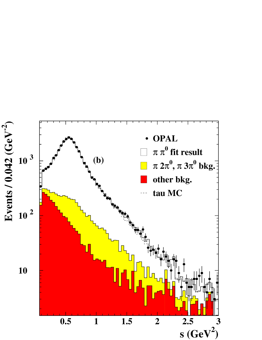
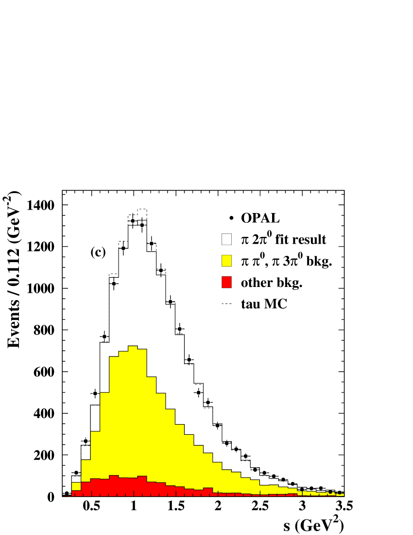
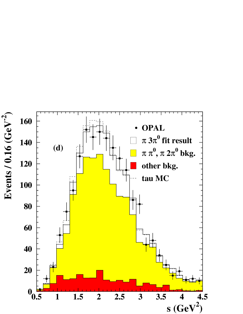
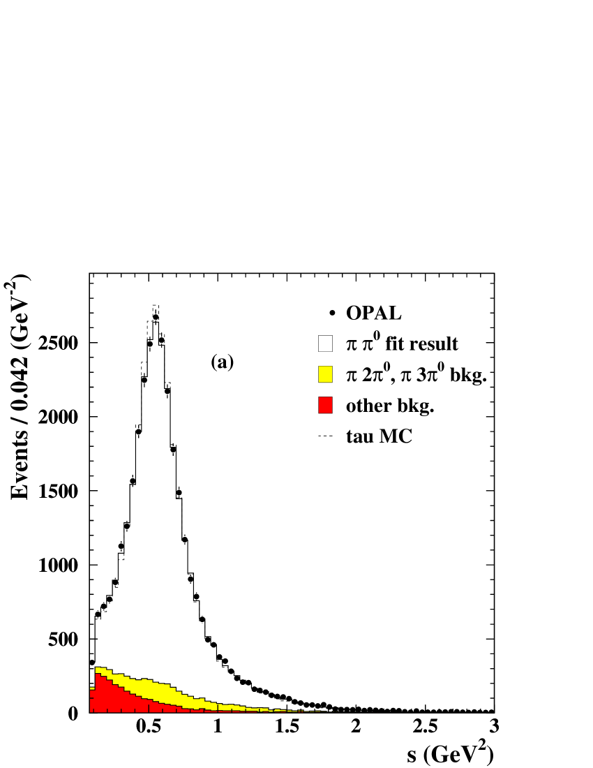
Figure 2: The measured s𝑚𝑒𝑎𝑠subscript𝑠𝑚𝑒𝑎𝑠\mathit{s_{\mathit{meas}}} spectra for 1-prong decays. Plots (a) and (b) are the ππ0𝜋superscript𝜋0\mathit{\mathrm{\pi}\mathrm{\pi^{0}}} channel, (c) and (d) are the π2π0𝜋2superscript𝜋0\mathit{\mathrm{\pi}2\mathrm{\pi^{0}}} and π3π0𝜋3superscript𝜋0\mathit{\mathrm{\pi}3\mathrm{\pi^{0}}} modes, respectively. The points denote OPAL data (statistical errors only). The open histograms show the fitted spectra after the regularized unfolding, refolded into detector space. The background contributions from simultaneously unfolded channels (correlated background) are shown as light grey areas while the background from other sources (uncorrelated background) is represented in dark grey.
Refer to caption
Refer to caption
Refer to caption
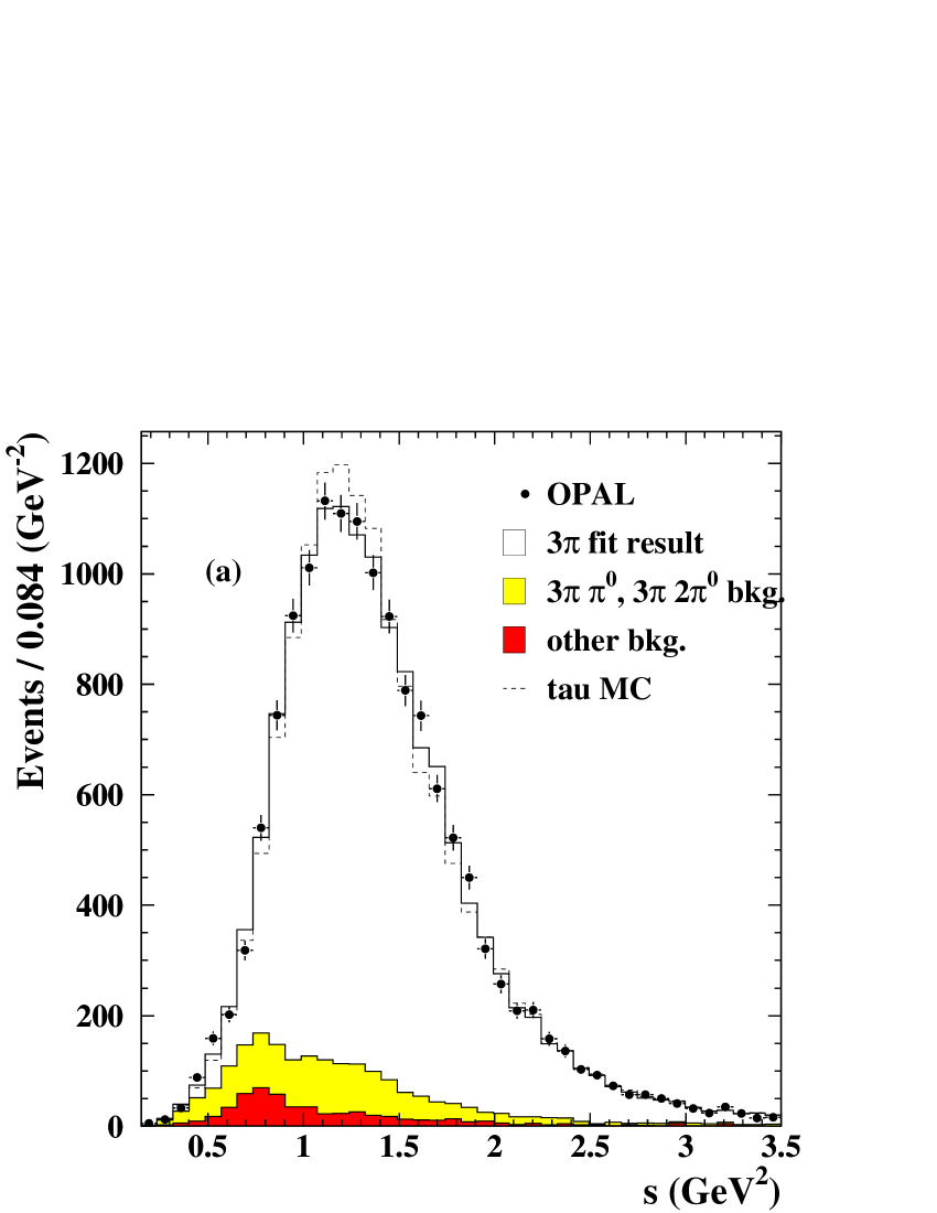
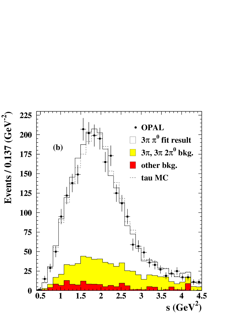
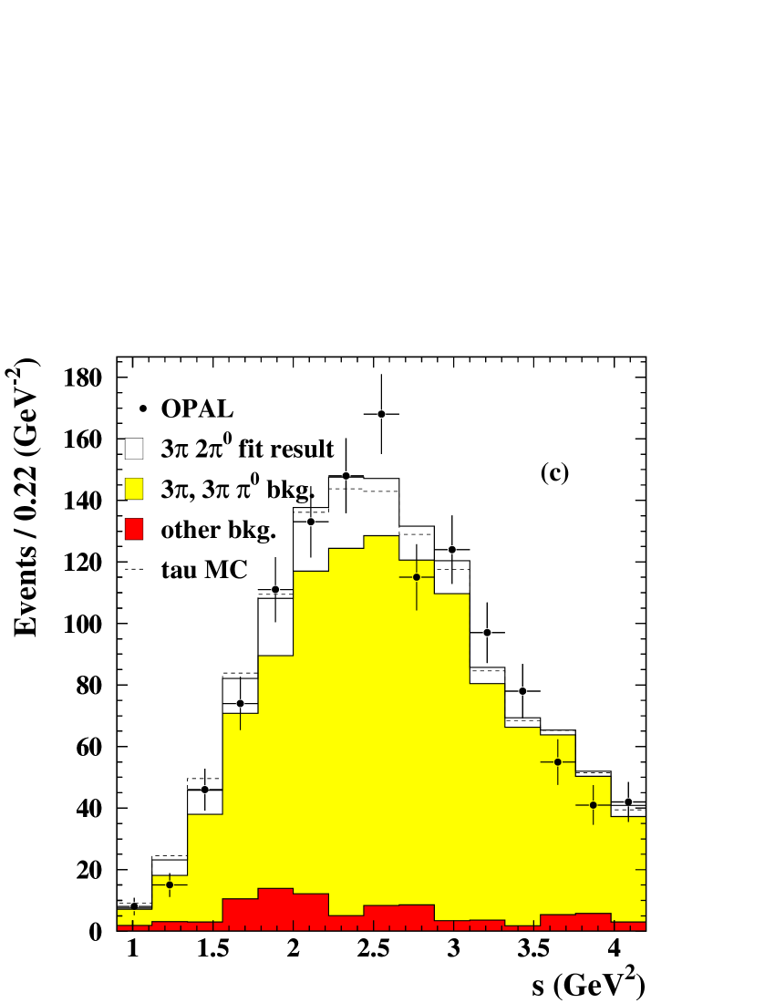
Figure 3: The measured s𝑚𝑒𝑎𝑠subscript𝑠𝑚𝑒𝑎𝑠\mathit{s_{\mathit{meas}}} spectra for 3-prong decays. Plot (a) is the 3π3𝜋\mathit{3\mathrm{\pi}} channel, (b) and (c) are the 3ππ03𝜋superscript𝜋0\mathit{3\mathrm{\pi}\mathrm{\pi^{0}}} and 3π2π03𝜋2superscript𝜋0\mathit{3\mathrm{\pi}2\mathrm{\pi^{0}}} modes, respectively. The points denote OPAL data (statistical errors only). The open histograms show the fitted spectra after the regularized unfolding, refolded into detector space. The background contributions from simultaneously unfolded channels (correlated background) are shown as light grey areas while the background from other sources (uncorrelated background) is represented in dark grey.

The selection efficiencies and background fractions from simultaneously unfolded channels (correlated background) and other τ𝜏\mathrm{\tau}- and non-τ𝜏\mathrm{\tau}-background sources (uncorrelated background) are listed in table 1.

channel efficiency correlated background uncorrelated background selected decays
ππ0𝜋superscript𝜋0\mathrm{\pi}\mathrm{\pi^{0}} (28.7±0.1)%percentplus-or-minus28.70.1(28.7\pm 0.1)\,\% (7.7±0.2)%percentplus-or-minus7.70.2(7.7\pm 0.2)\,\% (7.9±0.1)%percentplus-or-minus7.90.1(7.9\pm 0.1)\,\% 323163231632316
π2π0𝜋2superscript𝜋0\mathrm{\pi}2\mathrm{\pi^{0}} (18.8±0.1)%percentplus-or-minus18.80.1(18.8\pm 0.1)\,\% (45.0±0.6)%percentplus-or-minus45.00.6(45.0\pm 0.6)\,\% (8.4±0.1)%percentplus-or-minus8.40.1(8.4\pm 0.1)\,\% 138141381413814
π3π0𝜋3superscript𝜋0\mathrm{\pi}3\mathrm{\pi^{0}} (8.0±0.2)%percentplus-or-minus8.00.2(8.0\pm 0.2)\,\% (70.0±2.2)%percentplus-or-minus70.02.2(70.0\pm 2.2)\,\% (11.4±0.5)%percentplus-or-minus11.40.5(11.4\pm 0.5)\,\% 173817381738
3π3𝜋3\mathrm{\pi} (34.6±0.1)%percentplus-or-minus34.60.1(34.6\pm 0.1)\,\% (9.7±0.3)%percentplus-or-minus9.70.3(9.7\pm 0.3)\,\% (3.8±0.1)%percentplus-or-minus3.80.1(3.8\pm 0.1)\,\% 143211432114321
3ππ03𝜋superscript𝜋03\mathrm{\pi}\mathrm{\pi^{0}} (11.0±0.1)%percentplus-or-minus11.00.1(11.0\pm 0.1)\,\% (21.3±1.0)%percentplus-or-minus21.31.0(21.3\pm 1.0)\,\% (6.1±0.3)%percentplus-or-minus6.10.3(6.1\pm 0.3)\,\% 245524552455
3π2π03𝜋2superscript𝜋03\mathrm{\pi}2\mathrm{\pi^{0}} (8.3±0.4)%percentplus-or-minus8.30.4(8.3\pm 0.4)\,\% (82.3±2.9)%percentplus-or-minus82.32.9(82.3\pm 2.9)\,\% (7.1±0.5)%percentplus-or-minus7.10.5(7.1\pm 0.5)\,\% 125512551255
Table 1: Efficiencies, background fractions and total number of selected τ𝜏\mathrm{\tau} decays.

Figures 2 and 3 show the measured smeassubscript𝑠meass_{\rm meas} distributions of the six channels used in this analysis in comparison to the fitted signal after the regularized unfolding, and the Monte Carlo predictions.

The 3π3𝜋3\mathrm{\pi} spectrum shows a significant deviation from the shape predicted by the Monte Carlo (the dashed histogram) as has been observed in previous analyses of the 3π3𝜋3\mathrm{\pi} decay current [46]. There is also a slight deviation on the left side of the peak in the ππ0𝜋superscript𝜋0\mathrm{\pi}\mathrm{\pi^{0}} channel and in the upper tail region. The other modes are statistically consistent with their Monte Carlo predictions.

The χ2superscript𝜒2\chi^{2} values for the one-prong and three-prong fits after the regularization step are χ1pr.2/d.o.f.=94.0/109\chi^{2}_{\rm 1-pr.}/{\rm d.o.f.}=94.0/109 and χ3pr.2/d.o.f=71.4/69formulae-sequencesubscriptsuperscript𝜒23prdof71.469\chi^{2}_{\rm 3-pr.}/{\rm d.o.f}=71.4/69 leading to the χ2superscript𝜒2\chi^{2}-probabilities 0.850.850.85 and 0.400.400.40, respectively.

The unfolded distributions of the measured spectra are shown in figure 4.

Refer to caption
Refer to caption
Refer to caption
Refer to caption
Refer to caption
Refer to caption
Figure 4: The unfolded s𝑡𝑟𝑢𝑒subscript𝑠𝑡𝑟𝑢𝑒\mathit{s_{\mathit{true}}} spectra. Shown are the three vector channels (left) and the three axial-vector channels (right) together with the Monte Carlo prediction. There are strong correlations between the data points due to the unfolding. The plots (a),(d),(e) are the unfolded spectra of plots (a),(c),(d) in figure 2 and the plots (b),(c),(f) are the unfolded spectra of the plots (a),(b),(c) in figure 3. The error bars include statistical and systematic uncertainties.

The plotted data points are strongly correlated due to the unfolding procedure. The deviations from the Monte Carlo prediction seen in figures 2 and 3 are still present after the unfolding, most prominently in the ππ0𝜋superscript𝜋0\mathrm{\pi}\mathrm{\pi^{0}} and the 3π3𝜋3\mathrm{\pi} channel. The enhancement in the upper tail (see figures 2 (b) and 4 (a)) of the ππ0𝜋superscript𝜋0\mathrm{\pi}\mathrm{\pi^{0}} distribution can be explained within the Kühn–Santamaria model [47] by enlarging the fraction of ρ(1450)𝜌1450\mathrm{\rho(1450)}’s and ρ(1700)𝜌1700\mathrm{\rho(1700)}’s in the ρ𝜌\mathrm{\rho} decay amplitude. A similar correction to the three-pion current, modelled as a Breit–Wigner decay chain a1ρπ3πsubscripta1𝜌𝜋3𝜋\mathrm{a_{1}}\rightarrow\mathrm{\rho}\mathrm{\pi}\rightarrow 3\mathrm{\pi} [47] in the Monte Carlo, does not account for the observed discrepancy.

7 Systematic uncertainties

Possible origins for systematic effects on the reconstructed value for the squared hadronic mass, smeassubscript𝑠meass_{\rm meas}, come from the uncertainty in the energy scale for reconstructed photons and the uncertainty in the momentum scale for tracks, while the wrong choice of the regularization parameter ρ𝜌\rho in the unfolding can distort the unfolded distributions.

The energy resolution can be tested by measuring the invariant mass of the two photons from π0superscript𝜋0\mathrm{\pi^{0}} decays. A systematic shift in the observed mass in the data compared to the detector simulation can be translated into a scale factor for the reconstructed photon energies. Deviations of (0.5±0.9)MeVplus-or-minus0.50.9MeV(0.5\pm 0.9)\,{\rm MeV} for mπ0subscript𝑚superscript𝜋0m_{\mathrm{\pi^{0}}} have been observed between data and Monte Carlo (figure 1). This corresponds to an energy scale factor of 1.004±0.007plus-or-minus1.0040.0071.004\pm 0.007. The energies of the reconstructed photons in the Monte Carlo samples are varied by ±0.7%plus-or-minuspercent0.7\pm 0.7\,\% in order to estimate the systematic error due to this effect555Since the invariant two-photon mass depends also on the angle between the two photons, this energy scale factor accounts for systematic uncertainties in the energy resolution and the angular resolution of the ECAL..

The uncertainty in the momentum of the tracks have been studied using μ𝜇\mathrm{\mu} pairs. The Monte Carlo is corrected for observed deviations between data and Monte Carlo in the mean and the width of the momentum distribution. The momenta and the momentum resolution of all tracks in the Monte Carlo samples are scaled due to the uncertainties in these corrections, thus leading to the quoted systematic errors.

The damping parameter ρ𝜌\rho in the regularization step of the unfolding procedure is calculated from the number of effectively remaining spline coefficients after the regularization. This number is chosen so that the test conditions a) and b) given in section 5 are satisfied. The default value (161616 effective splines from 484848 total splines for the 1-prong fit and 161616 effective splines from 363636 total splines for the 3-prong fit) is varied by ±4plus-or-minus4\pm 4 for both fits, where the range is derived from Monte Carlo tests of the unfolding procedure: the tests consist of unfolding fake data samples in the ρππ0𝜌𝜋superscript𝜋0\mathrm{\rho}\rightarrow\mathrm{\pi}\mathrm{\pi^{0}} channel. The mass and the width of the ρ𝜌\mathrm{\rho} in the fake data samples at the generator level are different from the values used in the standard Monte Carlo which is used to create the response matrix. The allowed range of the damping parameter is then determined by comparing the unfolded fake data samples with their generator level distributions for different choices of the damping parameter, for which the test conditions a) and b) are satisfied. Within this range the unfolded distributions reproduce the mass spectrum of the modified ρ𝜌\mathrm{\rho} without biases towards the generator distribution of the standard Monte Carlo. The uncertainty due to the variation of the damping parameter is added as a systematic error on the unfolded results.

Uncertainties of statistical nature from the errors on the branching ratios (see table 2), the limited statistics of signal and background Monte Carlo samples, and on the efficiencies are incorporated in the unfolding procedure by adding them in quadrature to the statistical errors on the data.

Systematic effects related to photon and π0superscript𝜋0\mathrm{\pi^{0}} detection efficiency are largely covered by the systematic errors.

τντX𝜏subscript𝜈𝜏X\mathrm{\tau}\rightarrow\mathrm{\nu_{\tau}}{\rm X} B[%]B[\%] wVsubscript𝑤Vw_{\rm V} wAsubscript𝑤Aw_{\rm A} comment
eνeesubscript𝜈e\mathrm{e}\mathrm{\nu_{e}} 17.83±0.08plus-or-minus17.830.0817.83\pm 0.08
μνμ𝜇subscript𝜈𝜇\mathrm{\mu}\mathrm{\nu_{\mu}} 17.35±0.10plus-or-minus17.350.1017.35\pm 0.10
ππ0𝜋superscript𝜋0\mathrm{\pi}\mathrm{\pi^{0}} 25.24±0.16plus-or-minus25.240.1625.24\pm 0.16 1.01.01.0 0.00.00.0
3ππ03𝜋superscript𝜋03\mathrm{\pi}\mathrm{\pi^{0}} 4.26±0.09plus-or-minus4.260.09\phantom{0}4.26\pm 0.09 1.01.01.0 0.00.00.0 including ωπ𝜔𝜋\mathrm{\omega}\mathrm{\pi} and ωππ0𝜔𝜋superscript𝜋0\mathrm{\omega}\mathrm{\pi}\mathrm{\pi^{0}}
π3π0𝜋3superscript𝜋0\mathrm{\pi}3\mathrm{\pi^{0}} 1.14±0.14plus-or-minus1.140.14\phantom{0}1.14\pm 0.14 1.01.01.0 0.00.00.0
π𝜋\mathrm{\pi} 11.31±0.15plus-or-minus11.310.1511.31\pm 0.15 0.00.00.0 1.01.01.0
3π3𝜋3\mathrm{\pi} 9.26±0.12plus-or-minus9.260.12\phantom{0}9.26\pm 0.12 0.00.00.0 1.01.01.0 3h2KπK2π3h2K𝜋K2𝜋3\mathrm{h}-2\mathrm{K}\mathrm{\pi}-\mathrm{K}2\mathrm{\pi} including ωπ𝜔𝜋\mathrm{\omega}\mathrm{\pi}
π2π0𝜋2superscript𝜋0\mathrm{\pi}2\mathrm{\pi^{0}} 9.27±0.14plus-or-minus9.270.14\phantom{0}9.27\pm 0.14 0.00.00.0 1.01.01.0
3π2π03𝜋2superscript𝜋03\mathrm{\pi}2\mathrm{\pi^{0}} 0.50±0.05plus-or-minus0.500.05\phantom{0}0.50\pm 0.05 0.00.00.0 1.01.01.0 including ωππ0𝜔𝜋superscript𝜋0\mathrm{\omega}\mathrm{\pi}\mathrm{\pi^{0}} and ηππ0𝜂𝜋superscript𝜋0\mathrm{\eta}\mathrm{\pi}\mathrm{\pi^{0}}
5π5𝜋5\mathrm{\pi} 0.075±0.007plus-or-minus0.0750.007\phantom{0}0.075\pm 0.007 0.00.00.0 1.01.01.0 MC
π4π0𝜋4superscript𝜋0\mathrm{\pi}4\mathrm{\pi^{0}} 0.12±0.06plus-or-minus0.120.06\phantom{0}0.12\pm 0.06 0.00.00.0 1.01.01.0 MC
3π3π03𝜋3superscript𝜋03\mathrm{\pi}3\mathrm{\pi^{0}} 0.11±0.06plus-or-minus0.110.06\phantom{0}0.11\pm 0.06 1.01.01.0 0.00.00.0 MC
5ππ05𝜋superscript𝜋05\mathrm{\pi}\mathrm{\pi^{0}} 0.022±0.005plus-or-minus0.0220.005\phantom{0}0.022\pm 0.005 1.01.01.0 0.00.00.0 MC
KK0superscriptKK0\mathrm{K}\mathrm{K^{0}} 0.16±0.03plus-or-minus0.160.03\phantom{0}0.16\pm 0.03 1.01.01.0 0.00.00.0 MC
2Kπ2K𝜋2\mathrm{K}\mathrm{\pi} 0.10±0.03plus-or-minus0.100.03\phantom{0}0.10\pm 0.03 0.5±0.5plus-or-minus0.50.50.5\pm 0.5 0.5±0.5plus-or-minus0.50.50.5\pm 0.5 MC
2K0π2superscriptK0𝜋2\mathrm{K^{0}}\mathrm{\pi} 0.10±0.02plus-or-minus0.100.02\phantom{0}0.10\pm 0.02 0.5±0.5plus-or-minus0.50.50.5\pm 0.5 0.5±0.5plus-or-minus0.50.50.5\pm 0.5 MC
KK0π0superscriptKK0superscript𝜋0\mathrm{K}\mathrm{K^{0}}\mathrm{\pi^{0}} 0.14±0.03plus-or-minus0.140.03\phantom{0}0.14\pm 0.03 0.5±0.5plus-or-minus0.50.50.5\pm 0.5 0.5±0.5plus-or-minus0.50.50.5\pm 0.5 MC
ωπ𝜔𝜋\mathrm{\omega}\mathrm{\pi} 0.21±0.01plus-or-minus0.210.01\phantom{0}0.21\pm 0.01 1.01.01.0 0.20.2-0.2 MC excluding 3ππ03𝜋superscript𝜋03\mathrm{\pi}\mathrm{\pi^{0}}
ωππ0𝜔𝜋superscript𝜋0\mathrm{\omega}\mathrm{\pi}\mathrm{\pi^{0}} 0.046±0.007plus-or-minus0.0460.007\phantom{0}0.046\pm 0.007 0.250.25-0.25 1.01.01.0 excluding 3π2π03𝜋2superscript𝜋03\mathrm{\pi}2\mathrm{\pi^{0}}
ηππ0𝜂𝜋superscript𝜋0\mathrm{\eta}\mathrm{\pi}\mathrm{\pi^{0}} 0.17±0.03plus-or-minus0.170.03\phantom{0}0.17\pm 0.03 1.01.01.0 0.240.24-0.24 MC
XstrangesubscriptXstrange{\rm X}_{\rm strange} 2.67±0.14plus-or-minus2.670.14\phantom{0}2.67\pm 0.14
Table 2: Branching ratios for the hadron modes and lepton channels. Shown are the fitted values from the Particle Data Group [11] and the contributing weights for the vector and axial-vector current. Channels marked with MC are ‘generator-level’ Monte Carlo channels included in the spectra. Negative weights are used to subtract inclusively measured contributions from the wrong current.

8 Results

8.1 Moments of 𝑹𝝉subscript𝑹𝝉R_{\tau}

The unfolded spectra of the hadronic modes shown in figure 4 are normalized to their branching fractions and summed up to the vector and axial-vector spectra with their appropriate weights:

Rτ,V/Akl(s0)=0s0ds(1ss0)k(smτ2)lhV/AB(τhV/Aντ)B(τeνeντ)wV/ANV/AdNV/Ads,superscriptsubscript𝑅𝜏VA𝑘𝑙subscript𝑠0superscriptsubscript0subscript𝑠0differential-d𝑠superscript1𝑠subscript𝑠0𝑘superscript𝑠superscriptsubscript𝑚𝜏2𝑙subscriptsubscripthVA𝐵𝜏subscripthVAsubscript𝜈𝜏𝐵𝜏esubscript𝜈esubscript𝜈𝜏subscript𝑤VAsubscript𝑁VAdsubscript𝑁VAd𝑠R_{\mathrm{\tau},{\rm V/A}}^{kl}(s_{0})=\int\limits_{0}^{s_{0}}\mathrm{d}s\left(1-\frac{s}{s_{0}}\right)^{k}\left(\frac{s}{m_{\mathrm{\tau}}^{2}}\right)^{l}\sum_{\mathrm{h}_{\rm V/A}}\frac{B(\mathrm{\tau}\rightarrow\mathrm{h}_{\rm V/A}\mathrm{\nu_{\tau}})}{B(\mathrm{\tau}\rightarrow\mathrm{e}\mathrm{\nu_{e}}\mathrm{\nu_{\tau}})}\frac{w_{\rm V/A}}{N_{\rm V/A}}\frac{\mathrm{d}N_{\rm V/A}}{\mathrm{d}s}, (53)

where NV/Asubscript𝑁VAN_{\rm V/A} is the number of taus that decay into the hadron hV/AsubscripthVA\mathrm{h}_{\rm V/A} plus neutrino, and wV/Asubscript𝑤VAw_{\rm V/A} denotes the appropriate weight of the hadronic mode to the vector or axial-vector current. The branching ratios of the hadronic modes (and the lepton channels), together with their contributing weights for the vector and axial-vector spectra, are summarized in table 2.

The hadronic modes ωπ𝜔𝜋\mathrm{\omega}\mathrm{\pi}, ωππ0𝜔𝜋superscript𝜋0\mathrm{\omega}\mathrm{\pi}\mathrm{\pi^{0}} and ηππ0𝜂𝜋superscript𝜋0\mathrm{\eta}\mathrm{\pi}\mathrm{\pi^{0}} involve decays of ω𝜔\mathrm{\omega}’s and η𝜂\mathrm{\eta}’s, and do not conserve isospin symmetry, since their decay can occur via the electromagnetic interaction. Therefore, the unfolded distributions in the 3π3𝜋3\mathrm{\pi} mode, which is considered to belong to the axial-vector current, and in the 3ππ03𝜋superscript𝜋03\mathrm{\pi}\mathrm{\pi^{0}} mode, which belongs to the vector current, are contaminated by decays not belonging to the assigned currents (e.g. ωπ3π𝜔𝜋3𝜋\mathrm{\omega}\mathrm{\pi}\rightarrow 3\mathrm{\pi}), and thus need to be corrected. Since 71%similar-toabsentpercent71\sim 71\,\% of the 3π2π03𝜋2superscript𝜋03\mathrm{\pi}2\mathrm{\pi^{0}} mode consist of ωππ0𝜔𝜋superscript𝜋0\mathrm{\omega}\mathrm{\pi}\mathrm{\pi^{0}} decays, this channel is used for the ωππ0𝜔𝜋superscript𝜋0\mathrm{\omega}\mathrm{\pi}\mathrm{\pi^{0}} corrections. Corrections for the other ω𝜔\mathrm{\omega} and η𝜂\mathrm{\eta} modes are made with the Monte Carlo. Decay modes which are not reconstructed from the data have also to be included in the total vector and axial-vector spectra. Their distributions are taken from the Monte Carlo. The 2Kπ2K𝜋2\mathrm{K}\mathrm{\pi} modes contribute to both classes to an unknown amount. A weight of (50±50)%percentplus-or-minus5050(50\pm 50)\,\% is used for both currents and a correlation of 100%percent100-100\,\% between the vector and the axial-vector weights is assumed. The errors assigned to Monte Carlo spectra are taken to be ±100%plus-or-minuspercent100\pm 100\,\%, in order to take a possible mismodelling of the Monte Carlo into account.

moment kl𝑘𝑙kl RVklsuperscriptsubscript𝑅V𝑘𝑙R_{\rm V}^{kl} total error RAklsuperscriptsubscript𝑅A𝑘𝑙R_{\rm A}^{kl} total error
000000 1.7641.7641.764 ±0.016plus-or-minus0.016\pm 0.016 1.7201.7201.720 ±0.017plus-or-minus0.017\pm 0.017
101010 1.2641.2641.264 ±0.012plus-or-minus0.012\pm 0.012 1.2401.2401.240 ±0.013plus-or-minus0.013\pm 0.013
111111 0.29800.29800.2980 ±0.0034plus-or-minus0.0034\pm 0.0034 0.25100.25100.2510 ±0.0032plus-or-minus0.0032\pm 0.0032
121212 0.09420.09420.0942 ±0.0019plus-or-minus0.0019\pm 0.0019 0.10900.10900.1090 ±0.0019plus-or-minus0.0019\pm 0.0019
131313 0.04030.04030.0403 ±0.0016plus-or-minus0.0016\pm 0.0016 0.05180.05180.0518 ±0.0013plus-or-minus0.0013\pm 0.0013
Table 3: The measured moments RV/A𝑘𝑙superscriptsubscript𝑅𝑉𝐴𝑘𝑙\mathit{R_{V/A}^{kl}}, for 𝑘𝑙=00,10,11,12,13𝑘𝑙0010111213\mathit{kl=00,10,11,12,13}. The errors shown represent statistical and systematic uncertainties.
systematic errors
kl𝑘𝑙kl data stat. branching ratios MC stat. E𝐸E scale p𝑝p scale regularization
000000 ±0.016plus-or-minus0.016\pm 0.016
101010 ±0.005plus-or-minus0.005\pm 0.005 ±0.010plus-or-minus0.010\pm 0.010 ±0.004plus-or-minus0.004\pm 0.004 ±0.004plus-or-minus0.004\pm 0.004 ±0.001plus-or-minus0.001\pm 0.001 ±0.001plus-or-minus0.001\pm 0.001
VV\rm V 111111 ±0.0012plus-or-minus0.0012\pm 0.0012 ±0.0031plus-or-minus0.0031\pm 0.0031 ±0.0008plus-or-minus0.0008\pm 0.0008 ±0.0005plus-or-minus0.0005\pm 0.0005 ±0.0002plus-or-minus0.0002\pm 0.0002 ±0.0000plus-or-minus0.0000\pm 0.0000
121212 ±0.0006plus-or-minus0.0006\pm 0.0006 ±0.0016plus-or-minus0.0016\pm 0.0016 ±0.0004plus-or-minus0.0004\pm 0.0004 ±0.0007plus-or-minus0.0007\pm 0.0007 ±0.0000plus-or-minus0.0000\pm 0.0000 ±0.0001plus-or-minus0.0001\pm 0.0001
131313 ±0.0008plus-or-minus0.0008\pm 0.0008 ±0.0011plus-or-minus0.0011\pm 0.0011 ±0.0005plus-or-minus0.0005\pm 0.0005 ±0.0005plus-or-minus0.0005\pm 0.0005 ±0.0001plus-or-minus0.0001\pm 0.0001 ±0.0001plus-or-minus0.0001\pm 0.0001
000000 ±0.017plus-or-minus0.017\pm 0.017
101010 ±0.004plus-or-minus0.004\pm 0.004 ±0.012plus-or-minus0.012\pm 0.012 ±0.002plus-or-minus0.002\pm 0.002 ±0.002plus-or-minus0.002\pm 0.002 ±0.002plus-or-minus0.002\pm 0.002 ±0.003plus-or-minus0.003\pm 0.003
AA\rm A 111111 ±0.0010plus-or-minus0.0010\pm 0.0010 ±0.0029plus-or-minus0.0029\pm 0.0029 ±0.0007plus-or-minus0.0007\pm 0.0007 ±0.0003plus-or-minus0.0003\pm 0.0003 ±0.0002plus-or-minus0.0002\pm 0.0002 ±0.0004plus-or-minus0.0004\pm 0.0004
121212 ±0.0008plus-or-minus0.0008\pm 0.0008 ±0.0015plus-or-minus0.0015\pm 0.0015 ±0.0005plus-or-minus0.0005\pm 0.0005 ±0.0006plus-or-minus0.0006\pm 0.0006 ±0.0001plus-or-minus0.0001\pm 0.0001 ±0.0005plus-or-minus0.0005\pm 0.0005
131313 ±0.0007plus-or-minus0.0007\pm 0.0007 ±0.0008plus-or-minus0.0008\pm 0.0008 ±0.0004plus-or-minus0.0004\pm 0.0004 ±0.0004plus-or-minus0.0004\pm 0.0004 ±0.0002plus-or-minus0.0002\pm 0.0002 ±0.0003plus-or-minus0.0003\pm 0.0003
Table 4: Statistical and systematic uncertainties of the measured moments. The upper (lower) portion of the table contains the result for the vector (axial-vector) current.
VV\rm V 000000 101010 111111 121212
101010 727272
111111 878787 727272
121212 747474 141414 727272
131313 535353 1818-18 373737 909090
A\V\AV{\rm A}\backslash{\rm V} 000000 101010 111111 121212 131313
000000 222 999 00 88-8 88-8
101010 999 444 00 444 888
111111 55-5 22-2 77-7 77-7 44-4
121212 88-8 333 00 1212-12 1717-17
131313 1010-10 888 333 1616-16 2626-26
AA\rm A 000000 101010 111111 121212
101010 858585
111111 797979 565656
121212 646464 222222 858585
131313 515151 222 636363 949494
Table 5: Correlations between the measured moments RV/A𝑘𝑙superscriptsubscript𝑅𝑉𝐴𝑘𝑙\mathit{R_{V/A}^{kl}} in percent. The left (right) table gives the correlations between the moments of the vector (axial-vetor) current; the table in the middle shows the correlations between the moments of different currents.

The moments RV/Aklsuperscriptsubscript𝑅VA𝑘𝑙R_{\rm V/A}^{kl} are given in table 3. The errors on the moments are subdivided into statistical uncertainties due to the data statistics, the uncertainties comming from the branching ratio errors, and systematic uncertainties induced by the limited Monte Carlo statistics and the variations of the energy scale, the momentum scale, and the regularization parameter (table 4). Correlations between the moments are given in table 5.

8.2 Spectral functions

The vector and axial-vector spectral functions are given by inverting equation (1):

v/a(s)𝑣𝑎𝑠\displaystyle v/a(s) =\displaystyle= 2πImΠV/A(1)(s)2𝜋ImsuperscriptsubscriptΠVA1𝑠\displaystyle 2\pi\,{\rm Im}{\mit\Pi}_{\rm V/A}^{(1)}(s) (54)
=\displaystyle= mτ2[6SEW|Vud|2(1smτ2)2(1+2smτ2)]1superscriptsubscript𝑚𝜏2superscriptdelimited-[]6subscript𝑆EWsuperscriptsubscript𝑉ud2superscript1𝑠superscriptsubscript𝑚𝜏2212𝑠superscriptsubscript𝑚𝜏21\displaystyle m_{\mathrm{\tau}}^{2}\left[6S_{\rm EW}|V_{\rm ud}|^{2}\left(1-\frac{s}{m_{\mathrm{\tau}}^{2}}\right)^{2}\left(1+2\frac{s}{m_{\mathrm{\tau}}^{2}}\right)\right]^{-1}
×hV/AB(τhV/Aντ)B(τeνeντ)wV/ANV/AdNV/Ads,\displaystyle\times\sum_{\mathrm{h}_{\rm V/A}}\frac{B(\mathrm{\tau}\rightarrow\mathrm{h}_{\rm V/A}\mathrm{\nu_{\tau}})}{B(\mathrm{\tau}\rightarrow\mathrm{e}\mathrm{\nu_{e}}\mathrm{\nu_{\tau}})}\frac{w_{\rm V/A}}{N_{\rm V/A}}\frac{\mathrm{d}N_{\rm V/A}}{\mathrm{d}s},

where the sum is performed over hadronic final states hV/AsubscriptVAh_{\rm V/A} with angular momentum J=1𝐽1J=1.

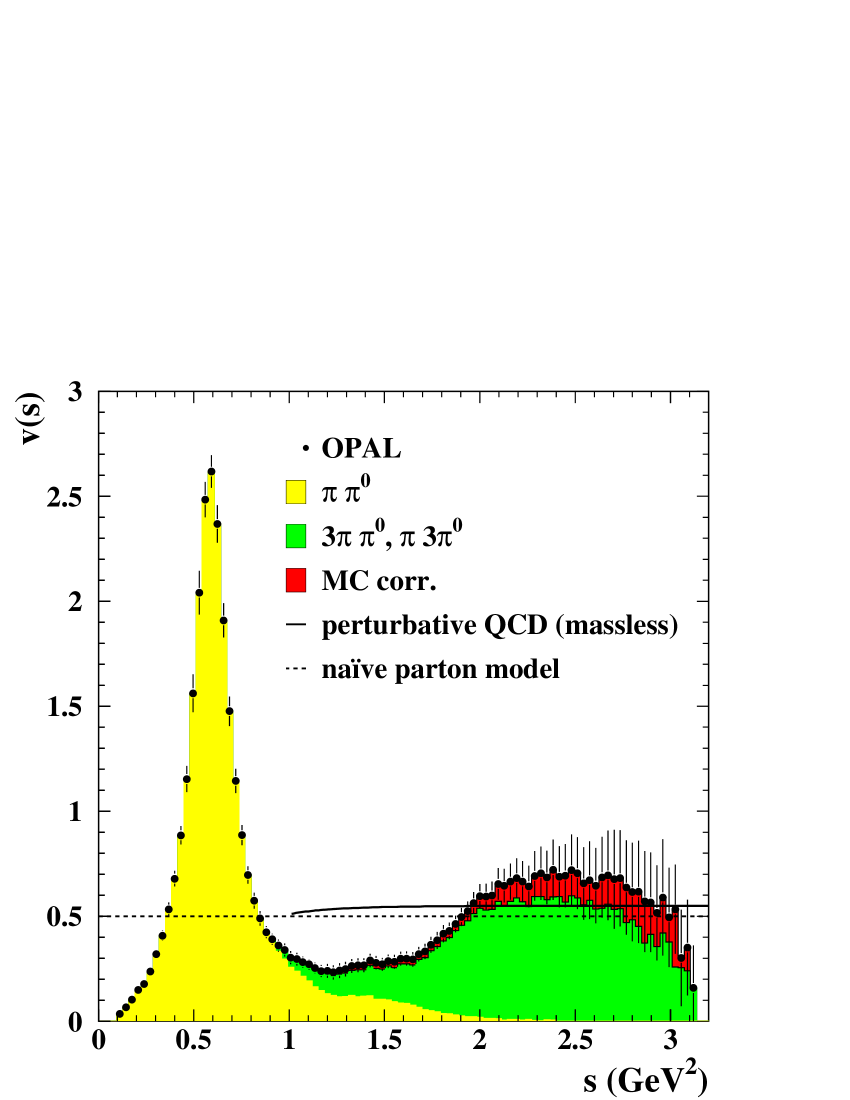
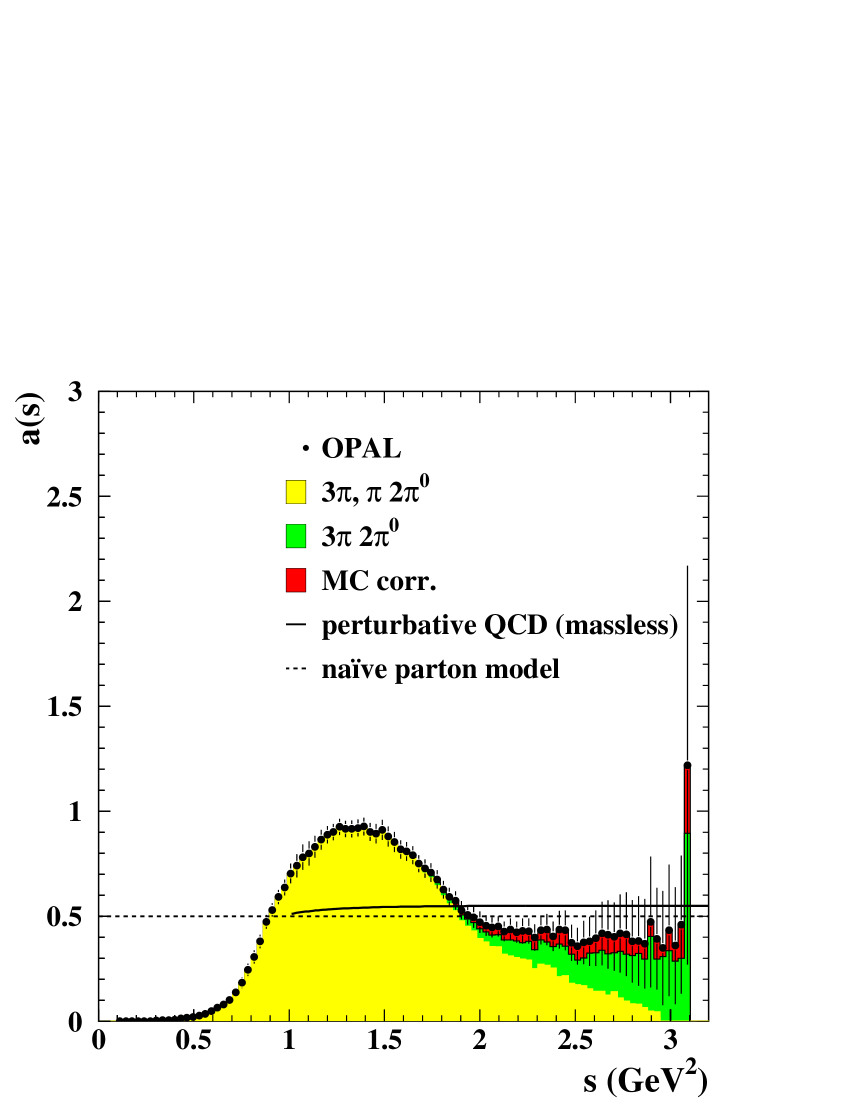
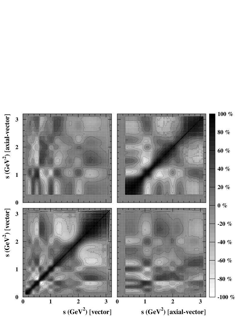
The spectral functions (and their correlations) are shown in figure 5 together with the flat naïve parton model prediction vnaı¨ve(s)=anaı¨ve(s)=1/2subscript𝑣na¨ıve𝑠subscript𝑎na¨ıve𝑠12v_{\rm na\ddot{\mathchar 16\relax}ve}(s)=a_{\rm na\ddot{\mathchar 16\relax}ve}(s)=1/2 and the prediction of perturbative QCD (massless) for αs(mZ2)=0.122subscript𝛼ssuperscriptsubscript𝑚Z20.122\alpha_{\rm s}(m_{\mathrm{Z}}^{2})=0.122 which increases the naïve prediction by 10%absentpercent10\approx 10\,\%. As a result of the regularized unfolding, the bin-to-bin correlations are of the order of +80%percent80+80\,\% (50%percent50-50\,\%) for bin distances of 0.1GeV20.1superscriptGeV20.1\,{\rm GeV^{2}} (1GeV2absent1superscriptGeV2\approx 1\,{\rm GeV}^{2}). The correlation between vector and axial-vector spectral function varies from 60%percent60-60\,\% to +60%percent60+60\,\%.

Refer to caption
Refer to caption
Refer to caption
Figure 5: The vector and axial-vector spectral functions. Shown are the sums of all contributing channels as data points (upper two plots). Some exclusive contributions are shown as shaded areas. The naïve parton model prediction is shown as dashed line, while the solid line depicts the perturbative, massless QCD prediction for αs(mZ2)=0.122subscript𝛼𝑠superscriptsubscript𝑚Z20.122\mathit{\alpha_{s}(m_{\mathrm{Z}}^{2})=0.122}. The error bars include statistical and systematic uncertainties. The pion pole is subtracted from the axial-vector spectrum. The lower plot shows the correlations of the two spectral functions in continuous gray-levels from white to black which correspond to the correlations in percent from 100%percent100\mathit{-100\,\%} to +100%percent100\mathit{+100\,\%}. The contour lines are drawn in equidistant steps of 20%percent20\mathit{20\,\%}.

Figure 6 shows the difference and the sum of the two measured spectral functions. The function v(s)a(s)𝑣𝑠𝑎𝑠v(s)-a(s) should vanish in the limit of perturbative, massless QCD. The deviation from this prediction, e.g. due to the ρ𝜌\mathrm{\rho} and a1subscripta1\mathrm{a_{1}} resonances, indicates the large sensitivity of this distribution to non-perturbative effects. The QCD prediction for v(s)+a(s)𝑣𝑠𝑎𝑠v(s)+a(s) which is 10%absentpercent10\approx 10\,\% above the naïve expectation v(s)+a(s)=1𝑣𝑠𝑎𝑠1v(s)+a(s)=1 as in figure 5 gives a reasonable description of the region s>1GeV2𝑠1superscriptGeV2s>1\,{\rm GeV}^{2}. The structure due to the narrow resonances in the region below s1GeV2similar-to-or-equals𝑠1superscriptGeV2s\simeq 1\,{\rm GeV}^{2} is however not described by perturbative QCD.

Refer to caption
Refer to caption
Figure 6: The difference (sum) of the spectral functions v(s)a(s)𝑣𝑠𝑎𝑠\mathit{v(s)-a(s)} (v(s)+a(s)𝑣𝑠𝑎𝑠\mathit{v(s)+a(s)}). The dashed line is the naïve parton model expectation and the solid lines depict the prediction of massless, perturbative QCD as in figure 5. For v(s)a(s)𝑣𝑠𝑎𝑠\mathit{v(s)-a(s)} both predictions are identically zero.

9 Measurement of the strong coupling 𝜶𝐬subscript𝜶𝐬\alpha_{\rm s}

Since the perturbative expansions for vector and axial-vector currents are identical while the non-perturbative parts have opposite sign but the same order of magnitude for both currents, two different fits are used for the extraction of αssubscript𝛼s\alpha_{\rm s} and the power corrections, respectively. The sum of vector and axial-vector moments is most sensitive to perturbative QCD and is used for the measurement of αssubscript𝛼s\alpha_{\rm s} (fit 1) while the separate moments of both currents are used to obtain the power corrections (fit 2). In addition to the moments listed in table 3 it is possible to include the measurements of the τ𝜏\mathrm{\tau} lifetime ττsubscript𝜏𝜏\tau_{\mathrm{\tau}} and the branching ratio Bμ=B(τμνμντ)subscript𝐵𝜇𝐵𝜏𝜇subscript𝜈𝜇subscript𝜈𝜏B_{\mathrm{\mu}}=B(\mathrm{\tau}\rightarrow\mathrm{\mu}\mathrm{\nu_{\mu}}\mathrm{\nu_{\tau}}) in fit 1 since each of them can be used to predict the total hadronic decay rate of the τ𝜏\mathrm{\tau} lepton:

Rτ(ττ)subscript𝑅𝜏subscript𝜏𝜏\displaystyle R_{\mathrm{\tau}}(\tau_{\mathrm{\tau}}) =\displaystyle= 1Γe1ττ1ΓμΓe,1subscriptΓe1subscript𝜏𝜏1subscriptΓ𝜇subscriptΓe\displaystyle\frac{1}{\Gamma_{\mathrm{e}}}\frac{1}{\tau_{\mathrm{\tau}}}-1-\frac{\Gamma_{\mathrm{\mu}}}{\Gamma_{\mathrm{e}}}, (55)
Rτ(Bμ)subscript𝑅𝜏subscript𝐵𝜇\displaystyle R_{\mathrm{\tau}}(B_{\mathrm{\mu}}) =\displaystyle= ΓμΓe1Bμ1ΓμΓe.subscriptΓ𝜇subscriptΓe1subscript𝐵𝜇1subscriptΓ𝜇subscriptΓe\displaystyle\frac{\Gamma_{\mathrm{\mu}}}{\Gamma_{\mathrm{e}}}\frac{1}{B_{\mathrm{\mu}}}-1-\frac{\Gamma_{\mathrm{\mu}}}{\Gamma_{\mathrm{e}}}. (56)

Both equations assume lepton universality so that the following equation holds:

Bμ=BeΓμΓe,subscript𝐵𝜇subscript𝐵esubscriptΓ𝜇subscriptΓeB_{\mathrm{\mu}}=B_{\mathrm{e}}\frac{\Gamma_{\mathrm{\mu}}}{\Gamma_{\mathrm{e}}}, (57)

with ΓμΓe=0.9726subscriptΓ𝜇subscriptΓe0.9726\frac{\Gamma_{\mathrm{\mu}}}{\Gamma_{\mathrm{e}}}=0.9726 [10] and Γe=4.03291013GeVsubscriptΓe4.0329superscript1013GeV\Gamma_{\mathrm{e}}=4.0329\cdot 10^{-13}\,{\rm GeV} [48, 10]. The non-strange decay rate of the τ𝜏\mathrm{\tau} lepton is then obtained by subtracting Rτ,s=Bs/Be=0.150±0.008subscript𝑅𝜏ssubscript𝐵ssubscript𝐵eplus-or-minus0.1500.008R_{\mathrm{\tau},{\rm s}}=B_{\rm s}/B_{\mathrm{e}}=0.150\pm 0.008 [11] from the weighted average Rτ(Bμ,ττ)subscript𝑅𝜏subscript𝐵𝜇subscript𝜏𝜏R_{\mathrm{\tau}}(B_{\mathrm{\mu}},\tau_{\mathrm{\tau}}) of Rτ(ττ)subscript𝑅𝜏subscript𝜏𝜏R_{\mathrm{\tau}}(\tau_{\mathrm{\tau}}) and Rτ(Bμ)subscript𝑅𝜏subscript𝐵𝜇R_{\mathrm{\tau}}(B_{\mathrm{\mu}})666 Rτ,ssubscript𝑅𝜏sR_{\mathrm{\tau},{\rm s}} is subtracted from Rτsubscript𝑅𝜏R_{\mathrm{\tau}}, since the induced dependency on the mass of the strange quark would lead to a larger uncertainty in the fits if Rτsubscript𝑅𝜏R_{\mathrm{\tau}} would be used instead.. In principle the electron branching ratio Besubscript𝐵eB_{\mathrm{e}} could also be used to determine Rτsubscript𝑅𝜏R_{\mathrm{\tau}} but this has a 96%percent9696\,\% correlation with Rτsubscript𝑅𝜏R_{\mathrm{\tau}} from the hadronic modes due to the correlations of the constrained branching ratios in [11].

Using the world average ττ=(291.0±1.5)fssubscript𝜏𝜏plus-or-minus291.01.5fs\tau_{\mathrm{\tau}}=(291.0\pm 1.5)\,{\rm fs} and the fitted value Bμ=0.1735±0.0010subscript𝐵𝜇plus-or-minus0.17350.0010B_{\mathrm{\mu}}=0.1735\pm 0.0010 [11] one gets:

Rτ(Bμ,ττ)Rτ,s=3.485±0.023.subscript𝑅𝜏subscript𝐵𝜇subscript𝜏𝜏subscript𝑅𝜏splus-or-minus3.4850.023R_{\mathrm{\tau}}(B_{\mathrm{\mu}},\tau_{\mathrm{\tau}})-R_{\mathrm{\tau},{\rm s}}=3.485\pm 0.023. (58)

From the vector and axial-vector decay rates in table 3 one gets the following value:

Rτ,V+Rτ,A=3.484±0.024.subscript𝑅𝜏Vsubscript𝑅𝜏Aplus-or-minus3.4840.024R_{\mathrm{\tau},{\rm V}}+R_{\mathrm{\tau},{\rm A}}=3.484\pm 0.024. (59)

In the first fit, four parameters are used to describe the five moments, leaving one degree of freedom for the fit: the strong coupling αs(mτ2)subscript𝛼ssuperscriptsubscript𝑚𝜏2\alpha_{\rm s}(m_{\mathrm{\tau}}^{2}), the gluon condensate αsπGGdelimited-⟨⟩subscript𝛼s𝜋𝐺𝐺\langle\frac{\alpha_{\rm s}}{\pi}\,GG\rangle and the dimension 6 and 8 contributions to the kl=00𝑘𝑙00kl=00 moments δV+A6superscriptsubscript𝛿VA6\delta_{\rm V+A}^{6}, δV+A8superscriptsubscript𝛿VA8\delta_{\rm V+A}^{8}. The second fit requires six parameters to predict ten moments (four degrees of freedom): αs(mτ2)subscript𝛼ssuperscriptsubscript𝑚𝜏2\alpha_{\rm s}(m_{\mathrm{\tau}}^{2}), αsπGGdelimited-⟨⟩subscript𝛼s𝜋𝐺𝐺\langle\frac{\alpha_{\rm s}}{\pi}\,GG\rangle and the power corrections δV6superscriptsubscript𝛿V6\delta_{\rm V}^{6}, δV8superscriptsubscript𝛿V8\delta_{\rm V}^{8}, δA6superscriptsubscript𝛿A6\delta_{\rm A}^{6} and δA8superscriptsubscript𝛿A8\delta_{\rm A}^{8}. The power corrections from the two fits can be compared via the following relation:

δV+AD=12(δVD+δAD).superscriptsubscript𝛿VA𝐷12superscriptsubscript𝛿V𝐷superscriptsubscript𝛿A𝐷\delta_{\rm V+A}^{D}=\frac{1}{2}\left(\delta_{\rm V}^{D}+\delta_{\rm A}^{D}\right). (60)

Further inputs for both fits are the quark masses for the three light quarks mu,d,ssubscript𝑚udsm_{\rm u,d,s}

mu=(8.7±1.5)MeV,md=(15.4±1.5)MeV,ms=(270±30)MeV,formulae-sequencesubscript𝑚uplus-or-minus8.71.5MeVformulae-sequencesubscript𝑚dplus-or-minus15.41.5MeVsubscript𝑚splus-or-minus27030MeVm_{\rm u}=(8.7\pm 1.5)\,{\rm MeV},\quad m_{\rm d}=(15.4\pm 1.5)\,{\rm MeV},\quad m_{\rm s}=(270\pm 30)\,{\rm MeV}, (61)

and the quark condensates ψ¯ψu,d,s=μu,d,s3subscriptdelimited-⟨⟩¯𝜓𝜓udssuperscriptsubscript𝜇uds3\langle\overline{\psi}\psi\rangle_{\rm u,d,s}=-\mu_{\rm u,d,s}^{3}, with

μu=μd=(189±7)MeV,μs=(160±10)MeV.formulae-sequencesubscript𝜇usubscript𝜇dplus-or-minus1897MeVsubscript𝜇splus-or-minus16010MeV\mu_{\rm u}=\mu_{\rm d}=(189\pm 7)\,{\rm MeV},\quad\mu_{\rm s}=(160\pm 10)\,{\rm MeV}. (62)

The values are taken from [4]. The error matrix of the moments is calculated from the experimental errors on the moments and their correlations (tables 3 and 5) and the theoretical error matrix calculated from the errors on the quark-masses and quark-condensates. The results from the fit to the sum of vector and axial-vector moments is given in table 6. The quoted errors are subdivided into a statistical error due to the data statistics, the uncertainty induced by the errors on the branching ratios, an experimental systematic error from the Monte Carlo statistics and the unfolding procedure, and a theoretical error including the uncertainties on quark masses, the variation of the O(αs4)𝑂superscriptsubscript𝛼s4O(\alpha_{\rm s}^{4}) coefficient, the renormalization scheme dependence, and the renormalization scale uncertainty. The strong coupling is most sensitive to the kl=00𝑘𝑙00kl=00 moment, and therefore the dominant contribution to the experimental uncertainty on αssubscript𝛼s\alpha_{\rm s} comes from the uncertainties on the branching ratios.

contributing errors
theory observable value data B𝐵B syst. theo. χ2/d.o.f.formulae-sequencesuperscript𝜒2dof\chi^{2}/{\rm d.o.f.}
αs(mτ2)subscript𝛼ssuperscriptsubscript𝑚𝜏2\alpha_{\rm s}(m_{\mathrm{\tau}}^{2}) 0.3480.348\phantom{+}0.348 ±0.002plus-or-minus0.002\pm 0.002 ±0.009plus-or-minus0.009\pm 0.009 ±0.002plus-or-minus0.002\pm 0.002 ±0.019plus-or-minus0.019\pm 0.019
αsπGG/GeV4delimited-⟨⟩subscript𝛼s𝜋𝐺𝐺superscriptGeV4\langle\frac{\alpha_{\rm s}}{\pi}\,GG\rangle/{\rm GeV^{4}} 0.0030.003-0.003 ±0.007plus-or-minus0.007\pm 0.007 ±0.007plus-or-minus0.007\pm 0.007 ±0.006plus-or-minus0.006\pm 0.006 ±0.005plus-or-minus0.005\pm 0.005
CIPT δV+A6superscriptsubscript𝛿VA6\delta_{\rm V+A}^{6} 0.00120.0012\phantom{+}0.0012 ±0.0034plus-or-minus0.0034\pm 0.0034 ±0.0033plus-or-minus0.0033\pm 0.0033 ±0.0029plus-or-minus0.0029\pm 0.0029 ±0.0006plus-or-minus0.0006\pm 0.0006 0.16/10.1610.16/1
δV+A8superscriptsubscript𝛿VA8\delta_{\rm V+A}^{8} 0.00100.0010-0.0010 ±0.0024plus-or-minus0.0024\pm 0.0024 ±0.0016plus-or-minus0.0016\pm 0.0016 ±0.0015plus-or-minus0.0015\pm 0.0015 ±0.0003plus-or-minus0.0003\pm 0.0003
αs(mτ2)subscript𝛼ssuperscriptsubscript𝑚𝜏2\alpha_{\rm s}(m_{\mathrm{\tau}}^{2}) 0.3240.324\phantom{+}0.324 ±0.001plus-or-minus0.001\pm 0.001 ±0.006plus-or-minus0.006\pm 0.006 ±0.002plus-or-minus0.002\pm 0.002 ±0.013plus-or-minus0.013\pm 0.013
αsπGG/GeV4delimited-⟨⟩subscript𝛼s𝜋𝐺𝐺superscriptGeV4\langle\frac{\alpha_{\rm s}}{\pi}\,GG\rangle/{\rm GeV^{4}} 0.0140.014\phantom{+}0.014 ±0.007plus-or-minus0.007\pm 0.007 ±0.006plus-or-minus0.006\pm 0.006 ±0.005plus-or-minus0.005\pm 0.005 ±0.013plus-or-minus0.013\pm 0.013
FOPT δV+A6superscriptsubscript𝛿VA6\delta_{\rm V+A}^{6} 0.00280.0028\phantom{+}0.0028 ±0.0034plus-or-minus0.0034\pm 0.0034 ±0.0034plus-or-minus0.0034\pm 0.0034 ±0.0030plus-or-minus0.0030\pm 0.0030 ±0.0068plus-or-minus0.0068\pm 0.0068 0.17/10.1710.17/1
δV+A8superscriptsubscript𝛿VA8\delta_{\rm V+A}^{8} 0.00150.0015-0.0015 ±0.0024plus-or-minus0.0024\pm 0.0024 ±0.0016plus-or-minus0.0016\pm 0.0016 ±0.0014plus-or-minus0.0014\pm 0.0014 ±0.0019plus-or-minus0.0019\pm 0.0019
αs(mτ2)subscript𝛼ssuperscriptsubscript𝑚𝜏2\alpha_{\rm s}(m_{\mathrm{\tau}}^{2}) 0.3060.306\phantom{+}0.306 ±0.001plus-or-minus0.001\pm 0.001 ±0.005plus-or-minus0.005\pm 0.005 ±0.001plus-or-minus0.001\pm 0.001 ±0.011plus-or-minus0.011\pm 0.011
αsπGG/GeV4delimited-⟨⟩subscript𝛼s𝜋𝐺𝐺superscriptGeV4\langle\frac{\alpha_{\rm s}}{\pi}\,GG\rangle/{\rm GeV^{4}} 0.0020.002-0.002 ±0.007plus-or-minus0.007\pm 0.007 ±0.007plus-or-minus0.007\pm 0.007 ±0.005plus-or-minus0.005\pm 0.005 ±0.002plus-or-minus0.002\pm 0.002
RCPT δV+A6superscriptsubscript𝛿VA6\delta_{\rm V+A}^{6} 0.00470.0047-0.0047 ±0.0036plus-or-minus0.0036\pm 0.0036 ±0.0040plus-or-minus0.0040\pm 0.0040 ±0.0032plus-or-minus0.0032\pm 0.0032 ±0.0011plus-or-minus0.0011\pm 0.0011 0.07/10.0710.07/1
δV+A8superscriptsubscript𝛿VA8\delta_{\rm V+A}^{8} 0.00010.0001-0.0001 ±0.0024plus-or-minus0.0024\pm 0.0024 ±0.0017plus-or-minus0.0017\pm 0.0017 ±0.0015plus-or-minus0.0015\pm 0.0015 ±0.0003plus-or-minus0.0003\pm 0.0003
Table 6: The result for αs(mτ2)subscript𝛼𝑠superscriptsubscript𝑚𝜏2\mathit{\alpha_{s}(m_{\tau}^{2})} and the non-perturbative parameters from the fit to the sum of vector and axial-vector moments. Shown are the values for the three different descriptions of the perturbative part of the moments (see text). The given errors correspond to the data statistics, the uncertainty due to the errors on the branching ratios B𝐵B, a systematic error from the Monte Carlo statistics, the energy scale, the momentum scale, and the unfolding, and a total theoretical uncertainty.

All three theories lead to similar χ2superscript𝜒2\chi^{2} values (see table 6) but the spread in the fitted values for αs(mτ2)subscript𝛼ssuperscriptsubscript𝑚𝜏2\alpha_{\rm s}(m_{\mathrm{\tau}}^{2}) exceeds the total uncertainties by a factor of two. A similar spread of the values for αs(mτ2)subscript𝛼𝑠superscriptsubscript𝑚𝜏2\alpha_{s}(m_{\mathrm{\tau}}^{2}) from the three models has also been observed in [49, 8], where RCPT has led to the lowest value and CIPT to the largest value in agreement with our results (table 6).

The differences in the statistical and systematic errors on αssubscript𝛼s\alpha_{\rm s} are induced by the scaling of the relative error with αssubscript𝛼s\alpha_{\rm s} and thus are compatible for the three fits. The theoretical uncertainties should also obey this scaling behavior: here the fits for FOPT and CIPT only include the uncertainty on the unknown K4subscript𝐾4K_{4} coefficient and hence cannot be compared to the RCPT result. Furthermore the uncertainty due to the variation of the renormalization scheme vanishes for RCPT. The impact on αssubscript𝛼s\alpha_{\rm s} from the various theoretical error sources is listed in table 7. The given errors correspond to the spread of the fitted values of αssubscript𝛼s\alpha_{\rm s} in fit 1 due to the unknown O(αs4)𝑂superscriptsubscript𝛼s4O\left(\alpha_{\rm s}^{4}\right) dependence K4=25±50subscript𝐾4plus-or-minus2550K_{4}=25\pm 50, the choice of renormalization scale 0.4μ2/mτ22.00.4superscript𝜇2superscriptsubscript𝑚𝜏22.00.4\leq\mu^{2}/m_{\mathrm{\tau}}^{2}\leq 2.0, the variation of the renormalization scheme parameterized with the third coefficient of the β𝛽\beta-function 0.0β3RS/β3MS¯2.00.0superscriptsubscript𝛽3RSsuperscriptsubscript𝛽3¯MS2.00.0\leq\beta_{3}^{\rm RS}/\beta_{3}^{\overline{\rm MS}}\leq 2.0, and the evolution of αs(mτ2)subscript𝛼ssuperscriptsubscript𝑚𝜏2\alpha_{\rm s}(m_{\mathrm{\tau}}^{2}) to the Z0superscriptZ0\mathrm{Z^{0}}-mass scale.

Δαs(mτ2)Δsubscript𝛼ssuperscriptsubscript𝑚𝜏2\Delta\alpha_{\rm s}(m_{\mathrm{\tau}}^{2}) Δαs(mZ2)Δsubscript𝛼ssuperscriptsubscript𝑚Z2\Delta\alpha_{\rm s}(m_{\mathrm{Z}}^{2})
error source CIPT FOPT RCPT CIPT FOPT RCPT
25K47525subscript𝐾475-25\leq K_{4}\leq 75 ±0.012plus-or-minus0.012\pm 0.012 ±0.006plus-or-minus0.006\pm 0.006 ±0.0013plus-or-minus0.0013\pm 0.0013 ±0.0007plus-or-minus0.0007\pm 0.0007
0.4μ2/mτ22.00.4superscript𝜇2superscriptsubscript𝑚𝜏22.00.4\leq\mu^{2}/m_{\mathrm{\tau}}^{2}\leq 2.0 ±0.006plus-or-minus0.006\pm 0.006 ±0.009plus-or-minus0.009\pm 0.009 ±0.011plus-or-minus0.011\pm 0.011 ±0.0005plus-or-minus0.0005\pm 0.0005 ±0.0009plus-or-minus0.0009\pm 0.0009 ±0.0015plus-or-minus0.0015\pm 0.0015
0.0β3RS/β3MS¯2.00.0superscriptsubscript𝛽3RSsuperscriptsubscript𝛽3¯MS2.00.0\leq\beta_{3}^{\rm RS}/\beta_{3}^{\overline{\rm MS}}\leq 2.0 ±0.015plus-or-minus0.015\pm 0.015 ±0.009plus-or-minus0.009\pm 0.009 ±0.000plus-or-minus0.000\pm 0.000 ±0.0009plus-or-minus0.0009\pm 0.0009 ±0.0005plus-or-minus0.0005\pm 0.0005 ±0.0005plus-or-minus0.0005\pm 0.0005
evolution ±0.0003plus-or-minus0.0003\pm 0.0003 ±0.0003plus-or-minus0.0003\pm 0.0003 ±0.0003plus-or-minus0.0003\pm 0.0003
Table 7: The theoretical uncertainties on the strong coupling constant. The errors correspond to the full spread of the fitted αssubscript𝛼𝑠\mathit{\alpha_{s}} values in fit 1 due to the variation of the parameters listed in the first column.

Although the total theoretical uncertainties on αssubscript𝛼s\alpha_{\rm s} are compatible for all three theories there is a major difference between FOPT and the two other models: the FOPT fit leads to a significant larger dependency of the non-perturbative parameters αsπGGdelimited-⟨⟩subscript𝛼s𝜋𝐺𝐺\langle\frac{\alpha_{\rm s}}{\pi}GG\rangle and δV+A6/8superscriptsubscript𝛿VA68\delta_{\rm V+A}^{6/8} on the theoretical uncertainties than CIPT and RCPT. The dominant effect comes from the variation of the renormalization scale μ2superscript𝜇2\mu^{2}. The statistical and systematic uncertainties on the power corrections are very similar for all three theories, agreeing with expectation. Figure 7 shows a comparison of Rτ,V(s0)+Rτ,A(s0)subscript𝑅𝜏Vsubscript𝑠0subscript𝑅𝜏Asubscript𝑠0R_{\mathrm{\tau},{\rm V}}(s_{0})+R_{\mathrm{\tau},{\rm A}}(s_{0}) as predicted from the three theories using the fit results at s0=mτ2subscript𝑠0superscriptsubscript𝑚𝜏2s_{0}=m_{\mathrm{\tau}}^{2} with the data. The Contour Improved prediction is consistent with the data from the τ𝜏\mathrm{\tau}-mass scale down to s01GeV2subscript𝑠01superscriptGeV2s_{0}\approx 1\,{\rm GeV}^{2} while FOPT and RCPT tend to predict too large values below s02GeV2subscript𝑠02superscriptGeV2s_{0}\approx 2\,{\rm GeV}^{2}.

Refer to caption
Figure 7: The non-strange hadronic decay rate of the τ𝜏\mathit{\mathrm{\tau}} lepton Rτ,V(s0)+Rτ,A(s0)subscript𝑅𝜏𝑉subscript𝑠0subscript𝑅𝜏𝐴subscript𝑠0\mathit{R_{\mathrm{\tau},{V}}(s_{0})+R_{\mathrm{\tau},{A}}(s_{0})} versus the upper integration limit s0subscript𝑠0s_{0}. The points in the upper plot denote OPAL data; the dashed, dashed-dotted and dotted curves represent the theoretical predictions of the three theories with the results from the fit to the moments at s0=mτ2subscript𝑠0superscriptsubscript𝑚𝜏2\mathit{s_{0}=m_{\mathrm{\tau}}^{2}} used as input. The lower plot shows the three theories normalized to the data. The three sets of dashed, dashed-dotted and dotted curves indicate central values and total experimental errors for each of the three theories. The errors on the data are shown as solid curves.

9.1 Evolution of 𝜶𝐬subscript𝜶𝐬\alpha_{\rm s} from 𝒎𝝉subscript𝒎𝝉m_{\mathrm{\tau}} to 𝒎𝐙subscript𝒎𝐙m_{\mathrm{Z}}

The value of the strong coupling at the mass scale of the τ𝜏\mathrm{\tau} lepton can be evolved up to the mass scale of the Z0superscriptZ0\mathrm{Z^{0}}. This is done by solving the four-loop β𝛽\beta-function given by equation (7) numerically in small steps from mτ2superscriptsubscript𝑚𝜏2m_{\mathrm{\tau}}^{2} to mZ2superscriptsubscript𝑚Z2m_{\mathrm{Z}}^{2} applying a three-loop matching condition [50] at the flavor thresholds for mc(mc)=(1.30±0.06)GeVsubscript𝑚csubscript𝑚cplus-or-minus1.300.06GeVm_{\rm c}(m_{\rm c})=(1.30\pm 0.06)\,{\rm GeV} and mb(mb)=(4.13±0.06)GeVsubscript𝑚bsubscript𝑚bplus-or-minus4.130.06GeVm_{\rm b}(m_{\rm b})=(4.13\pm 0.06)\,{\rm GeV} [50]. The evolution procedure induces an additional error of ±0.0003plus-or-minus0.0003\pm 0.0003 [50] on the strong coupling at the Z0superscriptZ0\mathrm{Z^{0}} mass. Using the CIPT result for αs(mτ2)subscript𝛼ssuperscriptsubscript𝑚𝜏2\alpha_{\rm s}(m_{\mathrm{\tau}}^{2}) and mZ=91.187GeVsubscript𝑚Z91.187GeVm_{\mathrm{Z}}=91.187\,{\rm GeV} the following value is obtained:

αs(mZ2)=0.1219±0.0010exp±0.0017theo±0.0003evol.subscript𝛼ssuperscriptsubscript𝑚Z2plus-or-minus0.1219subscript0.0010expsubscript0.0017theosubscript0.0003evol\alpha_{\rm s}(m_{\mathrm{Z}}^{2})=0.1219\pm 0.0010_{\rm exp}\pm 0.0017_{\rm theo}\pm 0.0003_{\rm evol}. (63)

The FOPT fit gives

αs(mZ2)=0.1191±0.0008exp±0.0013theo±0.0003evol.subscript𝛼ssuperscriptsubscript𝑚Z2plus-or-minus0.1191subscript0.0008expsubscript0.0013theosubscript0.0003evol\alpha_{\rm s}(m_{\mathrm{Z}}^{2})=0.1191\pm 0.0008_{\rm exp}\pm 0.0013_{\rm theo}\pm 0.0003_{\rm evol}. (64)

Finally RCPT gives:

αs(mZ2)=0.1169±0.0007exp±0.0015theo±0.0003evol.subscript𝛼ssuperscriptsubscript𝑚Z2plus-or-minus0.1169subscript0.0007expsubscript0.0015theosubscript0.0003evol\alpha_{\rm s}(m_{\mathrm{Z}}^{2})=0.1169\pm 0.0007_{\rm exp}\pm 0.0015_{\rm theo}\pm 0.0003_{\rm evol}. (65)

The different contributions to the theoretical uncertainties are listed in table 7. The results are in good agreement with the value obtained from fits to combined electroweak measurements at LEP and SLD [51]:

αs(mZ2)=0.120±0.003.subscript𝛼ssuperscriptsubscript𝑚Z2plus-or-minus0.1200.003\alpha_{\rm s}(m_{\mathrm{Z}}^{2})=0.120\pm 0.003. (66)

10 Measurement of dimension 6 and 8 operators

contributing errors
theory observable value data B𝐵B syst. theo. χ2/d.o.f.formulae-sequencesuperscript𝜒2dof\chi^{2}/{\rm d.o.f.}
αs(mτ2)subscript𝛼ssuperscriptsubscript𝑚𝜏2\alpha_{\rm s}(m_{\mathrm{\tau}}^{2}) 0.3470.347\phantom{+}0.347 ±0.001plus-or-minus0.001\pm 0.001 ±0.012plus-or-minus0.012\pm 0.012 ±0.002plus-or-minus0.002\pm 0.002 ±0.019plus-or-minus0.019\pm 0.019
αsπGG/GeV4delimited-⟨⟩subscript𝛼s𝜋𝐺𝐺superscriptGeV4\langle\frac{\alpha_{\rm s}}{\pi}\,GG\rangle/{\rm GeV^{4}} 0.0010.001\phantom{+}0.001 ±0.003plus-or-minus0.003\pm 0.003 ±0.006plus-or-minus0.006\pm 0.006 ±0.003plus-or-minus0.003\pm 0.003 ±0.004plus-or-minus0.004\pm 0.004
δV6superscriptsubscript𝛿V6\delta_{\rm V}^{6} 0.02560.0256\phantom{+}0.0256 ±0.0017plus-or-minus0.0017\pm 0.0017 ±0.0024plus-or-minus0.0024\pm 0.0024 ±0.0017plus-or-minus0.0017\pm 0.0017 ±0.0006plus-or-minus0.0006\pm 0.0006
CIPT δV8superscriptsubscript𝛿V8\delta_{\rm V}^{8} 0.00800.0080-0.0080 ±0.0010plus-or-minus0.0010\pm 0.0010 ±0.0007plus-or-minus0.0007\pm 0.0007 ±0.0005plus-or-minus0.0005\pm 0.0005 ±0.0002plus-or-minus0.0002\pm 0.0002 0.63/40.6340.63/4
δA6superscriptsubscript𝛿A6\delta_{\rm A}^{6} 0.01970.0197-0.0197 ±0.0016plus-or-minus0.0016\pm 0.0016 ±0.0022plus-or-minus0.0022\pm 0.0022 ±0.0019plus-or-minus0.0019\pm 0.0019 ±0.0010plus-or-minus0.0010\pm 0.0010
δA8superscriptsubscript𝛿A8\delta_{\rm A}^{8} 0.00410.0041\phantom{+}0.0041 ±0.0012plus-or-minus0.0012\pm 0.0012 ±0.0013plus-or-minus0.0013\pm 0.0013 ±0.0008plus-or-minus0.0008\pm 0.0008 ±0.0002plus-or-minus0.0002\pm 0.0002
αs(mτ2)subscript𝛼ssuperscriptsubscript𝑚𝜏2\alpha_{\rm s}(m_{\mathrm{\tau}}^{2}) 0.3230.323\phantom{+}0.323 ±0.001plus-or-minus0.001\pm 0.001 ±0.008plus-or-minus0.008\pm 0.008 ±0.002plus-or-minus0.002\pm 0.002 ±0.014plus-or-minus0.014\pm 0.014
αsπGG/GeV4delimited-⟨⟩subscript𝛼s𝜋𝐺𝐺superscriptGeV4\langle\frac{\alpha_{\rm s}}{\pi}\,GG\rangle/{\rm GeV^{4}} 0.0170.017\phantom{+}0.017 ±0.003plus-or-minus0.003\pm 0.003 ±0.004plus-or-minus0.004\pm 0.004 ±0.003plus-or-minus0.003\pm 0.003 ±0.010plus-or-minus0.010\pm 0.010
δV6superscriptsubscript𝛿V6\delta_{\rm V}^{6} 0.02710.0271\phantom{+}0.0271 ±0.0017plus-or-minus0.0017\pm 0.0017 ±0.0025plus-or-minus0.0025\pm 0.0025 ±0.0018plus-or-minus0.0018\pm 0.0018 ±0.0056plus-or-minus0.0056\pm 0.0056
FOPT δV8superscriptsubscript𝛿V8\delta_{\rm V}^{8} 0.00850.0085-0.0085 ±0.0010plus-or-minus0.0010\pm 0.0010 ±0.0007plus-or-minus0.0007\pm 0.0007 ±0.0005plus-or-minus0.0005\pm 0.0005 ±0.0012plus-or-minus0.0012\pm 0.0012 0.62/40.6240.62/4
δA6superscriptsubscript𝛿A6\delta_{\rm A}^{6} 0.01830.0183-0.0183 ±0.0016plus-or-minus0.0016\pm 0.0016 ±0.0023plus-or-minus0.0023\pm 0.0023 ±0.0019plus-or-minus0.0019\pm 0.0019 ±0.0052plus-or-minus0.0052\pm 0.0052
δA8superscriptsubscript𝛿A8\delta_{\rm A}^{8} 0.00360.0036\phantom{+}0.0036 ±0.0011plus-or-minus0.0011\pm 0.0011 ±0.0012plus-or-minus0.0012\pm 0.0012 ±0.0008plus-or-minus0.0008\pm 0.0008 ±0.0011plus-or-minus0.0011\pm 0.0011
αs(mτ2)subscript𝛼ssuperscriptsubscript𝑚𝜏2\alpha_{\rm s}(m_{\mathrm{\tau}}^{2}) 0.3050.305\phantom{+}0.305 ±0.001plus-or-minus0.001\pm 0.001 ±0.007plus-or-minus0.007\pm 0.007 ±0.001plus-or-minus0.001\pm 0.001 ±0.011plus-or-minus0.011\pm 0.011
αsπGG/GeV4delimited-⟨⟩subscript𝛼s𝜋𝐺𝐺superscriptGeV4\langle\frac{\alpha_{\rm s}}{\pi}\,GG\rangle/{\rm GeV^{4}} 0.0020.002\phantom{+}0.002 ±0.003plus-or-minus0.003\pm 0.003 ±0.005plus-or-minus0.005\pm 0.005 ±0.003plus-or-minus0.003\pm 0.003 ±0.001plus-or-minus0.001\pm 0.001
δV6superscriptsubscript𝛿V6\delta_{\rm V}^{6} 0.02020.0202\phantom{+}0.0202 ±0.0018plus-or-minus0.0018\pm 0.0018 ±0.0033plus-or-minus0.0033\pm 0.0033 ±0.0018plus-or-minus0.0018\pm 0.0018 ±0.0009plus-or-minus0.0009\pm 0.0009
RCPT δV8superscriptsubscript𝛿V8\delta_{\rm V}^{8} 0.00750.0075-0.0075 ±0.0010plus-or-minus0.0010\pm 0.0010 ±0.0008plus-or-minus0.0008\pm 0.0008 ±0.0005plus-or-minus0.0005\pm 0.0005 ±0.0002plus-or-minus0.0002\pm 0.0002 0.61/40.6140.61/4
δA6superscriptsubscript𝛿A6\delta_{\rm A}^{6} 0.02520.0252-0.0252 ±0.0017plus-or-minus0.0017\pm 0.0017 ±0.0032plus-or-minus0.0032\pm 0.0032 ±0.0020plus-or-minus0.0020\pm 0.0020 ±0.0006plus-or-minus0.0006\pm 0.0006
δA8superscriptsubscript𝛿A8\delta_{\rm A}^{8} 0.00470.0047\phantom{+}0.0047 ±0.0012plus-or-minus0.0012\pm 0.0012 ±0.0013plus-or-minus0.0013\pm 0.0013 ±0.0008plus-or-minus0.0008\pm 0.0008 ±0.0001plus-or-minus0.0001\pm 0.0001
Table 8: The fit result for αssubscript𝛼𝑠\mathit{\alpha_{s}} and the power corrections from the combined fit to vector and axial-vector moments. The given errors correspond to the data statistics, the uncertainty due to the errors on the branching ratios B𝐵B, a systematic error from the Monte Carlo statistics, the energy scale, the momentum scale, and the unfolding, and a total theoretical uncertainty.
αs(mτ2)subscript𝛼ssuperscriptsubscript𝑚𝜏2\alpha_{\rm s}(m_{\mathrm{\tau}}^{2}) αsπGGdelimited-⟨⟩subscript𝛼s𝜋𝐺𝐺\left\langle\frac{\alpha_{\rm s}}{\pi}GG\right\rangle δV6superscriptsubscript𝛿V6\delta_{\rm V}^{6} δA6superscriptsubscript𝛿A6\delta_{\rm A}^{6} δV8superscriptsubscript𝛿V8\delta_{\rm V}^{8}
αsπGGdelimited-⟨⟩subscript𝛼s𝜋𝐺𝐺\left\langle\frac{\alpha_{\rm s}}{\pi}GG\right\rangle 5757-57
δV6superscriptsubscript𝛿V6\delta_{\rm V}^{6} 5555-55 9999\phantom{+}99
δA6superscriptsubscript𝛿A6\delta_{\rm A}^{6} 6161-61 9696\phantom{+}96 9696\phantom{+}96
δV8superscriptsubscript𝛿V8\delta_{\rm V}^{8} 4141\phantom{+}41 9292-92 9090-90 8484-84
δA8superscriptsubscript𝛿A8\delta_{\rm A}^{8} 4242\phantom{+}42 8787-87 8686-86 7777-77 8989\phantom{+}89
Table 9: Correlations between the QCD parameters from the fit to the moments of the vector and axial-vector current in percent. The given numbers are taken from the CIPT fit result.
Refer to caption
Figure 8: The power corrections of dimension 6 to Rτ,V/Asubscript𝑅𝜏𝑉𝐴\mathit{R_{\mathrm{\tau},{V/A}}}. Shown are the one and two standard deviation contours of the correlated result for the vector and axial-vector current (CIPT) including experimental and theoretical uncertainties. The solid line indicates the theoretical prediction given in [4].

The results from fit 2 where the separate moments of the vector current and axial-vector current are used are given in table 8. In contrast to αssubscript𝛼s\alpha_{\rm s} where the error is dominated by the theoretical uncertainties, the power corrections are almost independent of the theoretical uncertainties for CIPT and RCPT. As mentioned in section 9, this is not the case for the FOPT fit which leads to theoretical errors of the order of (or even larger than) the experimental errors. Due to the correlated unfolding of vector and axial-vector spectra a strong positive correlation between the power corrections of the vector and axial vector current of the same dimension is observed. The power corrections of different dimension but for the same current are anti-correlated. All correlations of the fit parameters for CIPT are summarized in table 9. The fitted values of the strong coupling constant in both fits are in excellent agreement for all three models. The experimental error on αssubscript𝛼s\alpha_{\rm s} from this fit is larger than in fit 1 as the additional information from the τ𝜏\mathrm{\tau} lifetime and the branching ratio B(τμνμντ)𝐵𝜏𝜇subscript𝜈𝜇subscript𝜈𝜏B(\mathrm{\tau}\rightarrow\mathrm{\mu}\mathrm{\nu_{\mu}}\mathrm{\nu_{\tau}}) is omitted. Using equation (60), the separate and total power corrections are also in good agreement for all three models. As in fit 1 all three theories give similar χ2superscript𝜒2\chi^{2} values in the fit to the exclusive moments. The theoretical uncertainties behave similarly in fit 1 and fit 2. The sum of all power corrections δnonpert,V/Asubscript𝛿nonpertVA\delta_{\rm non\mathchar 45\relax pert,V/A} and δnonpert,V+Asubscript𝛿nonpertVA\delta_{\rm non\mathchar 45\relax pert,V+A} to Rτ,V/Asubscript𝑅𝜏VAR_{\mathrm{\tau},{\rm V/A}} and Rτ,V+Rτ,Asubscript𝑅𝜏Vsubscript𝑅𝜏AR_{\mathrm{\tau},{\rm V}}+R_{\mathrm{\tau},{\rm A}} including the dimension 2 quark-mass correction and the dimension 4 correction obtained from the fitted gluon condensate are:

0.0172±0.0026CIPTplus-or-minus0.01720.0026CIPT\displaystyle\phantom{+}0.0172\pm 0.0026\quad{\rm CIPT}
δnonpert,Vsubscript𝛿nonpertV\displaystyle\delta_{\rm non\mathchar 45\relax pert,V} =\displaystyle= 0.0187±0.0054FOPTplus-or-minus0.01870.0054FOPT\displaystyle\phantom{+}0.0187\pm 0.0054\quad{\rm FOPT}
0.0124±0.0033RCPT,plus-or-minus0.01240.0033RCPT\displaystyle\phantom{+}0.0124\pm 0.0033\quad{\rm RCPT},
0.0219±0.0026CIPTplus-or-minus0.02190.0026CIPT\displaystyle-0.0219\pm 0.0026\quad{\rm CIPT}
δnonpert,Asubscript𝛿nonpertA\displaystyle\delta_{\rm non\mathchar 45\relax pert,A} =\displaystyle= 0.0204±0.0050FOPTplus-or-minus0.02040.0050FOPT\displaystyle-0.0204\pm 0.0050\quad{\rm FOPT}
0.0266±0.0032RCPT,plus-or-minus0.02660.0032RCPT\displaystyle-0.0266\pm 0.0032\quad{\rm RCPT},
0.0024±0.0025CIPTplus-or-minus0.00240.0025CIPT\displaystyle-0.0024\pm 0.0025\quad{\rm CIPT}
δnonpert,V+Asubscript𝛿nonpertVA\displaystyle\delta_{\rm non\mathchar 45\relax pert,V+A} =\displaystyle= 0.0009±0.0051FOPTplus-or-minus0.00090.0051FOPT\displaystyle-0.0009\pm 0.0051\quad{\rm FOPT}
0.0071±0.0031RCPT,plus-or-minus0.00710.0031RCPT\displaystyle-0.0071\pm 0.0031\quad{\rm RCPT},

where the errors include experimental and theoretical uncertainties. Thus all three theories lead to non-perturbative corrections to Rτ,Vsubscript𝑅𝜏VR_{\mathrm{\tau},{\rm V}} (Rτ,Asubscript𝑅𝜏AR_{\mathrm{\tau},{\rm A}}) of the order 1.6%percent1.61.6\,\% (2.3%percent2.3-2.3\,\%), while a large cancellation of both contributions leads to a total non-perturbative correction to Rτ,V+Rτ,Asubscript𝑅𝜏Vsubscript𝑅𝜏AR_{\mathrm{\tau},{\rm V}}+R_{\mathrm{\tau},{\rm A}} which is compatible with zero and therefore allows a precise measurement of the strong coupling constant in fit 1. The numbers in table 8 can be compared to the estimates given in [4]:

αsπGG/GeV4delimited-⟨⟩subscript𝛼s𝜋𝐺𝐺superscriptGeV4\displaystyle\langle\frac{\alpha_{\rm s}}{\pi}\,GG\rangle/{\rm GeV^{4}} =\displaystyle= 0.02±0.01,plus-or-minus0.020.01\displaystyle\phantom{+}0.02\pm 0.01,
δV6superscriptsubscript𝛿V6\displaystyle\delta_{\rm V}^{6} =\displaystyle= 0.024±0.013,plus-or-minus0.0240.013\displaystyle\phantom{+}0.024\pm 0.013, (70)
δA6superscriptsubscript𝛿A6\displaystyle\delta_{\rm A}^{6} =\displaystyle= 0.038±0.020,plus-or-minus0.0380.020\displaystyle-0.038\pm 0.020,
δV/A8superscriptsubscript𝛿VA8\displaystyle\delta_{\rm V/A}^{8} similar-to-or-equals\displaystyle\simeq 0.0001.0.0001\displaystyle-0.0001.

Only the power corrections of dimension 8 seem to be underestimated, while the other estimates are in good agreement with the measured values. Figure 8 shows the two power corrections of dimension 6 (CIPT) together with the theoretical prediction given in [4].

11 Test of the ‘running’ of 𝜶𝐬subscript𝜶𝐬\alpha_{\rm s}

The fit to the sum of vector and axial-vector moments (fit 1) can be extended to lower values of s0subscript𝑠0s_{0}, thus giving a correlated measurement of the strong coupling at different scales. Four equidistant values for s0subscript𝑠0s_{0} between 1.3GeV21.3superscriptGeV21.3\,{\rm GeV}^{2} and mτ2superscriptsubscript𝑚𝜏2m_{\mathrm{\tau}}^{2} are used. In addition to the five moments at s0=mτ2subscript𝑠0superscriptsubscript𝑚𝜏2s_{0}=m_{\mathrm{\tau}}^{2} the integrated differential decay rate Rτ,V00(s0)+Rτ,A00(s0)superscriptsubscript𝑅𝜏V00subscript𝑠0superscriptsubscript𝑅𝜏A00subscript𝑠0R_{\mathrm{\tau},{\rm V}}^{00}(s_{0})+R_{\mathrm{\tau},{\rm A}}^{00}(s_{0}) for each additional s0subscript𝑠0s_{0} value is included in the fit (see figure 7).

For the extraction of the ‘running’ of αssubscript𝛼s\alpha_{\rm s} the number of fit parameters is increased to include the strong coupling αs(s0)subscript𝛼ssubscript𝑠0\alpha_{\rm s}(s_{0}) for each s0subscript𝑠0s_{0} value below mτ2superscriptsubscript𝑚𝜏2m_{\mathrm{\tau}}^{2}. The result can be examined with the four-loop β𝛽\beta-function. This is shown in figure 9, where the β𝛽\beta-function has been refitted for all three sets of αssubscript𝛼s\alpha_{\rm s} values. The values at s0=1.3GeV2subscript𝑠01.3superscriptGeV2s_{0}=1.3\,{\rm GeV^{2}} were not included in the fit. A comparison of these values with the predicted ‘running’ shows good agreement in case of CIPT, while a weaker ‘running’ as predicted by the β𝛽\beta-function is preferred by the FOPT and the RCPT values.
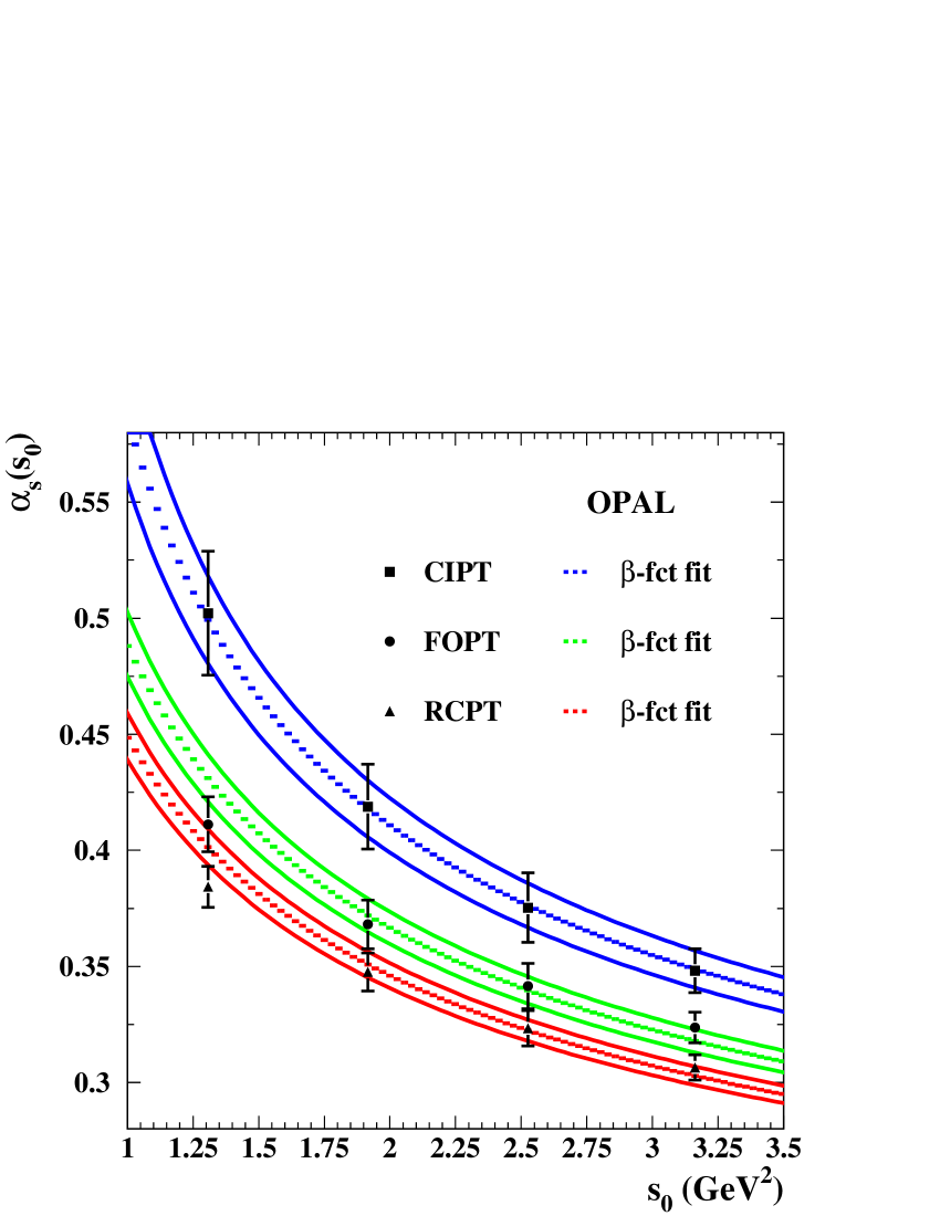
Refer to caption
Figure 9: The ‘running’  of the strong coupling. The three sets of αssubscript𝛼𝑠\mathit{\alpha_{s}} values are shown as data points. The error bars include statistical and systematic uncertainties. The dashed curves represent the predictions of the 4-loop β𝛽\mathit{\beta}-function obtained from fits to the three sets of αssubscript𝛼𝑠\mathit{\alpha_{s}} values not including the values αs(1.3𝐺𝑒𝑉2)subscript𝛼𝑠1.3superscript𝐺𝑒𝑉2\mathit{\alpha_{s}(1.3\,{GeV}^{2})}. The solid lines depict the errors from the fits.

Figures 7 and 9 can be regarded as tests of the validity of the OPE for s0subscript𝑠0s_{0} values below mτ2superscriptsubscript𝑚𝜏2m_{\mathrm{\tau}}^{2}. It has been questioned if the definition of Rτ(s0)subscript𝑅𝜏subscript𝑠0R_{\mathrm{\tau}}(s_{0}) is still valid in this region [4], since the endpoint s=s0𝑠subscript𝑠0s=s_{0} is no longer suppressed by the (1s/mτ2)2superscript1𝑠superscriptsubscript𝑚𝜏22(1-s/m_{\mathrm{\tau}}^{2})^{2} term in front of the spectral function (see equation (1)). By defining the hadronic decay rate for a hypothetical τsuperscript𝜏\mathrm{\tau}^{\prime} with a mass of mτ=s0subscript𝑚superscript𝜏subscript𝑠0m_{\mathrm{\tau}^{\prime}}=\sqrt{s_{0}} and inserting mτsubscript𝑚superscript𝜏m_{\mathrm{\tau}^{\prime}} for mτsubscript𝑚𝜏m_{\mathrm{\tau}} in equation (1) one gets [8]:

Rτ,V/A(s0)=12πSEW|Vud|20s0dss0(1ss0)2[(1+2ss0)ImΠV/A(1)(s)+ImΠV/A(0)(s)],subscript𝑅superscript𝜏VAsubscript𝑠012𝜋subscript𝑆EWsuperscriptsubscript𝑉ud2superscriptsubscript0subscript𝑠0d𝑠subscript𝑠0superscript1𝑠subscript𝑠02delimited-[]12𝑠subscript𝑠0ImsuperscriptsubscriptΠVA1𝑠ImsuperscriptsubscriptΠVA0𝑠R_{\mathrm{\tau}^{\prime},{\rm V/A}}(s_{0})=12\pi S_{\rm EW}|V_{\rm ud}|^{2}\int\limits_{0}^{s_{0}}{\frac{\mathrm{d}s}{s_{0}}\left(1-\frac{s}{s_{0}}\right)^{2}\left[\left(1+2\frac{s}{s_{0}}\right){\rm Im}{\mit\Pi}_{\rm V/A}^{(1)}(s)+{\rm Im}{\mit\Pi}_{\rm V/A}^{(0)}(s)\right]}, (71)

obeying the same quadratic suppression of the endpoint on the real s𝑠s-axis as Rτ,V/A(mτ2)subscript𝑅𝜏VAsuperscriptsubscript𝑚𝜏2R_{\mathrm{\tau},{\rm V/A}}(m_{\mathrm{\tau}}^{2}). Figure 10 shows the sum Rτ,V(s0)+Rτ,A(s0)subscript𝑅superscript𝜏Vsubscript𝑠0subscript𝑅superscript𝜏Asubscript𝑠0R_{\mathrm{\tau}^{\prime},{\rm V}}(s_{0})+R_{\mathrm{\tau}^{\prime},{\rm A}}(s_{0}) versus the upper integration limit s0subscript𝑠0s_{0}. The error band for CIPT in the lower plot shows that the uncertainties increase below s01.5GeV2similar-to-or-equalssubscript𝑠01.5superscriptGeV2s_{0}\simeq 1.5\,{\rm GeV}^{2} compared to the error in the lower plot of figure 7. While the error on Rτ(s0)subscript𝑅𝜏subscript𝑠0R_{\mathrm{\tau}}(s_{0}) is dominated by the uncertainty of the perturbative expansion, the error on Rτ(s0)subscript𝑅superscript𝜏subscript𝑠0R_{\mathrm{\tau}^{\prime}}(s_{0}) originates mainly from its dependency on the non-perturbative parts. In contrast to Rτsubscript𝑅𝜏R_{\mathrm{\tau}} where these power corrections stay constant for all s0subscript𝑠0s_{0} (see equation (2.2)) they increase with powers of 1/s01subscript𝑠01/s_{0} as s0subscript𝑠0s_{0} decreases in the case of Rτsubscript𝑅superscript𝜏R_{\mathrm{\tau}^{\prime}}. As the errors are large for small values of s0subscript𝑠0s_{0} little can be said about this region.

Refer to caption
Figure 10: The non-strange hadronic decay rate of a hypothetical τsuperscript𝜏\mathit{\mathrm{\tau}^{\prime}} lepton with mτ2=s0superscriptsubscript𝑚superscript𝜏2subscript𝑠0\mathit{m_{\mathrm{\tau}^{\prime}}^{2}=s_{0}} versus the upper integration limit s0subscript𝑠0\mathit{s_{0}}. The points in the upper plot denote OPAL data; the dashed, dashed-dotted and dotted curves represent the theoretical predictions of the three theories with the results from the fit to the moments at s0=mτ2subscript𝑠0superscriptsubscript𝑚𝜏2\mathit{s_{0}=m_{\mathrm{\tau}}^{2}} used as input. The lower plot shows the three theories normalized to the data. The three dashed curves indicate central values and total experimental errors for CIPT. The dashed-dotted and dotted curves show central values for FOPT and RCPT. The errors for FOPT and RCPT are similar to the CIPT errors and omitted from the plot. The errors on the data are shown as solid lines.

12 QCD sum rules

Refer to caption
Refer to caption
Refer to caption
Refer to caption
Figure 11: QCD sum rules. Equations (72)–(75) are shown in the plots (a)–(d). Shown are the integrals versus the upper integration limit as shaded bands. The chiral prediction is given by the lines (±1σplus-or-minus1𝜎\mathit{\pm 1\,\sigma} when two lines are present).

Weighted integrals over the difference of the two measured spectral functions shown in figure 6 can be compared to the chiral predictions of QCD sum rules:

I1(s0)subscript𝐼1subscript𝑠0\displaystyle I_{1}(s_{0}) =\displaystyle= 14π20s0ds(v(s)a(s))=fπ2,14superscript𝜋2superscriptsubscript0subscript𝑠0differential-d𝑠𝑣𝑠𝑎𝑠superscriptsubscript𝑓𝜋2\displaystyle\frac{1}{4\pi^{2}}\int\limits_{0}^{s_{0}}\mathrm{d}s\,\left(v(s)-a(s)\right)=f_{\pi}^{2}, (72)
I2(s0)subscript𝐼2subscript𝑠0\displaystyle I_{2}(s_{0}) =\displaystyle= 14π20s0dss(v(s)a(s))=0,14superscript𝜋2superscriptsubscript0subscript𝑠0differential-d𝑠𝑠𝑣𝑠𝑎𝑠0\displaystyle\frac{1}{4\pi^{2}}\int\limits_{0}^{s_{0}}\mathrm{d}s\,s\,\left(v(s)-a(s)\right)=0, (73)
I3(s0)subscript𝐼3subscript𝑠0\displaystyle I_{3}(s_{0}) =\displaystyle= 14π20s0dss(v(s)a(s))=fπ2rπ23FA,14superscript𝜋2superscriptsubscript0subscript𝑠0d𝑠𝑠𝑣𝑠𝑎𝑠superscriptsubscript𝑓𝜋2delimited-⟨⟩superscriptsubscript𝑟𝜋23subscript𝐹A\displaystyle\frac{1}{4\pi^{2}}\int\limits_{0}^{s_{0}}\frac{\mathrm{d}s}{s}\,\left(v(s)-a(s)\right)=f_{\pi}^{2}\,\frac{\langle r_{\pi}^{2}\rangle}{3}-F_{\rm A}, (74)
I4(s0)subscript𝐼4subscript𝑠0\displaystyle I_{4}(s_{0}) =\displaystyle= 14π20s0dsslnsλ2(v(s)a(s))=4πfπ23α(mπ±2mπ02).14superscript𝜋2superscriptsubscript0subscript𝑠0differential-d𝑠𝑠ln𝑠superscript𝜆2𝑣𝑠𝑎𝑠4𝜋superscriptsubscript𝑓𝜋23𝛼superscriptsubscript𝑚superscript𝜋plus-or-minus2superscriptsubscript𝑚superscript𝜋02\displaystyle\frac{1}{4\pi^{2}}\int\limits_{0}^{s_{0}}\mathrm{d}s\,s\,{\rm ln}\frac{s}{\lambda^{2}}\,\left(v(s)-a(s)\right)=-\frac{4\pi f_{\pi}^{2}}{3\,\alpha}\left(m_{\pi^{\pm}}^{2}-m_{\pi^{0}}^{2}\right). (75)

Here the right hand side of each equation is understood to be the chiral prediction in the limit s0subscript𝑠0s_{0}\rightarrow\infty. Equation (72) is known as the first Weinberg sum rule [52], assuming that the only scalar contribution is given by the pion pole which is related to the pion decay constant fπ=(92.4±0.26)MeVsubscript𝑓𝜋plus-or-minus92.40.26MeVf_{\mathrm{\pi}}=(92.4\pm 0.26)\,{\rm MeV} [11]. The second Weinberg sum rule [52] is given in equation (73). The Das–Mathur–Okubo (DMO) sum rule [53] is given by equation (74). Its asymptotic prediction is a function of the pion decay constant fπsubscript𝑓𝜋f_{\mathrm{\pi}}, the mean square of the pion charge radius rπ2=(0.439±0.008)fm2delimited-⟨⟩superscriptsubscript𝑟𝜋2plus-or-minus0.4390.008superscriptfm2\langle r_{\mathrm{\pi}}^{2}\rangle=(0.439\pm 0.008)\,{\rm fm}^{2} [54] and the axial-vector form factor of the pion FA=0.0058±0.0008subscript𝐹Aplus-or-minus0.00580.0008F_{\rm A}=0.0058\pm 0.0008 [11]777Our definitions of FAsubscript𝐹AF_{\rm A} and fπ2superscriptsubscript𝑓𝜋2f_{\mathrm{\pi}}^{2} differ by a factor of 1/2121/2 from those given in [11], and equation (75) gives the electromagnetic mass difference of pions [55]. Note that equation (75) does not depend on the cut-off value λ𝜆\lambda by virtue of the second Weinberg sum rule.

The saturation of these four sum rules is tested taking into account the full correlations between the measured spectral functions. The plots of figure 11 show the measured values of the integrals I1subscript𝐼1I_{1}-I4subscript𝐼4I_{4} as error bands including all experimental uncertainties versus the upper integration limit. The asymptotic predictions are drawn as thin lines denoting the present ±1σplus-or-minus1𝜎\pm 1\,\sigma ranges.

All four sum rules appear to be saturated at the τ𝜏\mathrm{\tau}-mass scale within their errors. However, due to the small phase space near the τ𝜏\mathrm{\tau}-mass which appears in the denominator of the spectral functions these errors are very large except for the DMO sum rule where the 1/s1𝑠1/s factor suppresses the high energy tail. The value of equation (74) at s0=mτ2subscript𝑠0superscriptsubscript𝑚𝜏2s_{0}=m_{\mathrm{\tau}}^{2} is:

I3(mτ2)=(26.3±1.8)103,subscript𝐼3superscriptsubscript𝑚𝜏2plus-or-minus26.31.8superscript103I_{3}(m_{\mathrm{\tau}}^{2})=(26.3\pm 1.8)\cdot 10^{-3}, (76)

where the error covers all experimental uncertainties.

12.1 Pion polarizability

Assuming that the DMO sum rule shown in figure 11 (c) is already saturated at the τ𝜏\mathrm{\tau}-mass scale, its value can be used to predict the electric polarizability of the charged pion as proposed in [56]:

αE=αmπ±(rπ23I3fπ2).subscript𝛼E𝛼subscript𝑚superscript𝜋plus-or-minusdelimited-⟨⟩superscriptsubscript𝑟𝜋23subscript𝐼3superscriptsubscript𝑓𝜋2\alpha_{\rm E}=\frac{\alpha}{m_{\pi^{\pm}}}\left(\frac{\langle r_{\pi}^{2}\rangle}{3}-\frac{I_{3}}{f_{\pi}^{2}}\right). (77)

Using the result from the previous section for the DMO sum rule (equation (76)) one gets:

αE=(2.71±0.88)104fm3,subscript𝛼Eplus-or-minus2.710.88superscript104superscriptfm3\alpha_{\rm E}=(2.71\pm 0.88)\cdot 10^{-4}\,{\rm fm}^{3}, (78)

which is in good agreement with the value αE=(2.64±0.36)104fm3subscript𝛼Eplus-or-minus2.640.36superscript104superscriptfm3\alpha_{\rm E}=(2.64\pm 0.36)\cdot 10^{-4}\,{\rm fm}^{3}, derived in [56].

13 Summary

Measurements of the spectral functions of the vector current and the axial-vector current and their applications in QCD have been presented. Within the framework of the Operator Product Expansion, a simultaneous determination of the strong coupling constant αssubscript𝛼s\alpha_{\rm s} and non-perturbative correction terms has been performed. The sum of Rτ,Vsubscript𝑅𝜏VR_{\mathrm{\tau},{\rm V}} and Rτ,Asubscript𝑅𝜏AR_{\mathrm{\tau},{\rm A}} was found to involve a large cancellation of the non-perturbative terms and thus has been used together with the τ𝜏\mathrm{\tau} lifetime and the branching ratio B(τμνμντ)𝐵𝜏𝜇subscript𝜈𝜇subscript𝜈𝜏B(\mathrm{\tau}\rightarrow\mathrm{\mu}\mathrm{\nu_{\mu}}\mathrm{\nu_{\tau}}) to give a precise measurement of the strong coupling constant. CIPT has led to the value

αs(mτ2)=0.348±0.009exp±0.019theo,subscript𝛼ssuperscriptsubscript𝑚𝜏2plus-or-minus0.348subscript0.009expsubscript0.019theo\alpha_{\rm s}(m_{\mathrm{\tau}}^{2})=0.348\pm 0.009_{\rm exp}\pm 0.019_{\rm theo},

at the τ𝜏\mathrm{\tau}-mass scale and

αs(mZ2)=0.1219±0.0010exp±0.0017theosubscript𝛼ssuperscriptsubscript𝑚Z2plus-or-minus0.1219subscript0.0010expsubscript0.0017theo\alpha_{\rm s}(m_{\mathrm{Z}}^{2})=0.1219\pm 0.0010_{\rm exp}\pm 0.0017_{\rm theo}

at the Z0superscriptZ0\mathrm{Z^{0}}-mass scale, where the first error stems from the experimental uncertainties and the second error originates from the theoretical uncertainties. The values obtained for αs(mZ2)subscript𝛼ssuperscriptsubscript𝑚Z2\alpha_{\rm s}(m_{\mathrm{Z}}^{2}) using FOPT or RCPT are 2.3%percent2.32.3\,\% and 4.1%percent4.14.1\,\% smaller, respectively.

The total amount of non-perturbative corrections to Rτ,Vsubscript𝑅𝜏VR_{\mathrm{\tau},{\rm V}} (Rτ,Asubscript𝑅𝜏AR_{\mathrm{\tau},{\rm A}}) was found to be (1.6±0.4)%percentplus-or-minus1.60.4(1.6\pm 0.4)\,\% ((2.3±0.4)%percentplus-or-minus2.30.4(-2.3\pm 0.4)\,\%), while the correction on the sum of Rτ,Vsubscript𝑅𝜏VR_{\mathrm{\tau},{\rm V}} and Rτ,Asubscript𝑅𝜏AR_{\mathrm{\tau},{\rm A}} due to non-perturbative QCD is found to be only (0.3±0.4)%percentplus-or-minus0.30.4(-0.3\pm 0.4)\,\%. Here the errors include all experimental and theoretical uncertainties.

Assuming the validity of the Operator Product Expansion for energy scales below the τ𝜏\mathrm{\tau} mass a test of the ‘running’ of the strong coupling between s01.3GeV2similar-to-or-equalssubscript𝑠01.3superscriptGeV2s_{0}\simeq 1.3\,{\rm GeV}^{2} and s0=mτ2subscript𝑠0superscriptsubscript𝑚𝜏2s_{0}=m_{\mathrm{\tau}}^{2} has been performed. A good agreement between the predicted ‘running’ from the 444-loop β𝛽\beta-function and the fitted αssubscript𝛼s\alpha_{\rm s} values has been observed for CIPT.

The saturation of QCD sum rules at the τ𝜏\mathrm{\tau}-mass scale has been tested, yielding a measurement of the pion polarizability of αE=(2.71±0.88)104fm3subscript𝛼Eplus-or-minus2.710.88superscript104superscriptfm3\alpha_{\rm E}=(2.71\pm 0.88)\cdot 10^{-4}\,{\rm fm}^{3} as determined from the DMO sum rule.

Acknowledgements

We particularly wish to thank the SL Division for the efficient operation of the LEP accelerator at all energies and for their continuing close cooperation with our experimental group. We thank our colleagues from CEA, DAPNIA/SPP, CE-Saclay for their efforts over the years on the time-of-flight and trigger systems which we continue to use. In addition to the support staff at our own institutions we are pleased to acknowledge the
Department of Energy, USA,
National Science Foundation, USA,
Particle Physics and Astronomy Research Council, UK,
Natural Sciences and Engineering Research Council, Canada,
Israel Science Foundation, administered by the Israel Academy of Science and Humanities,
Minerva Gesellschaft,
Benoziyo Center for High Energy Physics,
Japanese Ministry of Education, Science and Culture (the Monbusho) and a grant under the Monbusho International Science Research Program,
German Israeli Bi-national Science Foundation (GIF),
Bundesministerium für Bildung, Wissenschaft, Forschung und Technologie, Germany,
National Research Council of Canada,
Research Corporation, USA,
Hungarian Foundation for Scientific Research, OTKA T-016660, T023793 and OTKA F-023259.
We also wish to thank A. Höcker, J.H. Kühn, C.J. Maxwell and M. Neubert for numerous helpful discussions about the theoretical peculiarities of the subject.

References

  • [1] E. Braaten, Phys. Rev. Lett. 60 (1988) 1606.
  • [2] E. Braaten, Phys. Rev. D39 (1989) 1458.
  • [3] S. Narison and A. Pich, Phys. Lett. B211 (1988) 183.
  • [4] E. Braaten, S. Narison, and A. Pich, Nucl. Phys. B373 (1992) 581.
  • [5] F. Le Diberder and A. Pich, Phys. Lett. B286 (1992) 147.
  • [6] P.N. Burrows, MIT-LNS-97-272 (1997), Invited talk at 17th International Conference on Physics in Collision, Bristol (1997).
  • [7] ALEPH Collaboration, D. Buskulic et al., Phys. Lett. B307 (1993) 209.
  • [8] ALEPH Collaboration, R. Barate et al., CERN-EP-98-012 (1998).
  • [9] CLEO Collaboration, T. Coan et al., Phys. Lett. B356 (1995) 580.
  • [10] W.J. Marciano and A. Sirlin, Phys. Rev. Lett. 61 (1988) 1815.
  • [11] Particle Data Group, R.M. Barnett et al., Phys. Rev. D54 (1996) 1, and 1997 off-year partial update for the 1998 edition available on the PDG WWW pages (URL: http://pdg.lbl.gov/).
  • [12] F. Le Diberder and A. Pich, Phys. Lett. B289 (1992) 165.
  • [13] E. Braaten and C.S. Li, Phys. Rev. D42 (1990) 3888.
  • [14] T. van Ritbergen, J.A.M. Vermaseren, and S.A. Larin, Phys. Lett. B400 (1997) 379.
  • [15] M. Neubert, Nucl. Phys. B463 (1996) 511.
  • [16] C.N. Lovett-Turner and C.J. Maxwell, Nucl. Phys. B452 (1995) 188.
  • [17] C.J. Maxwell and D.G. Tonge, Nucl. Phys. B481 (1996) 681.
  • [18] K.G. Chetyrkin, A.L. Kataev, and F.V. Tkachev, Phys. Lett. B85 (1979) 277.
  • [19] M. Dine and J. Sapirstein, Phys. Rev. Lett. 43 (1979) 668.
  • [20] W. Celmaster and R.J. Gonsalves, Phys. Rev. Lett. 44 (1980) 560.
  • [21] S.G. Gorishnii, A.L. Kataev, and S.A. Larin, Phys. Lett. B259 (1991) 144.
  • [22] L.R. Surguladze and M.A. Samuel, Phys. Rev. Lett. 66 (1991) 560, Erratum: ibid. 66 (1991) 2416.
  • [23] A. Pich, FTUV-97-03 (1996), Invited talk at 20th Johns Hopkins Workshop on Current Problems in Particle Theory, Heidelberg (1996).
  • [24] A.L. Kataev and V.V. Starshenko, Mod. Phys. Lett. A10 (1995) 235.
  • [25] K.G. Wilson, Phys. Rev. 179 (1969) 1499.
  • [26] M.A. Shifman, A.I. Vainshtein, and V.I. Zakharov, Nucl. Phys. B147 (1979) 385.
  • [27] M.A. Shifman, A.I. Vainshtein, and V.I. Zakharov, Nucl. Phys. B147 (1979) 448.
  • [28] M.A. Shifman, A.I. Vainshtein, and V.I. Zakharov, Nucl. Phys. B147 (1979) 519.
  • [29] OPAL Collaboration, K. Ahmet et al., Nucl. Instrum. Methods A305 (1991) 275.
  • [30] P. Allport et al., Nucl. Instrum. Methods A324 (1993) 34.
  • [31] P. Allport et al., Nucl. Instrum. Methods A346 (1994) 476.
  • [32] M. Hauschild et al., Nucl. Instrum. Methods A314 (1992) 74.
  • [33] S. Jadach, B.F.L. Ward, and Z. Wa̧s, Comp. Phys. Comm. 79 (1994) 503.
  • [34] S. Jadach, Z. Wa̧s, R. Decker, and J.H. Kühn, Comp. Phys. Comm. 76 (1993) 361.
  • [35] R. Brun et al., CERN-DD/EE/84-1 (1989).
  • [36] J. Allison et al., Nucl. Instrum. Methods A317 (1992) 47.
  • [37] T. Sjöstrand, Comp. Phys. Comm. 82 (1994) 74.
  • [38] M. Bohm, A. Denner, and W. Hollik, Nucl. Phys. B304 (1988) 687.
  • [39] F.A. Beerends, R. Kleiss, and W. Hollik, Nucl. Phys. B304 (1988) 712.
  • [40] R. Battacharya, J. Smith, and G. Grammer, Phys. Rev. D15 (1977) 3267.
  • [41] J. Smith, J.A.M. Vermaseren, and G. Grammer, Phys. Rev. D15 (1977) 3280.
  • [42] OPAL Collaboration, R. Akers et al., Phys. Lett. B328 (1994) 207.
  • [43] OPAL Collaboration, J. Allison et al., Z. Phys. C66 (1995) 31.
  • [44] G.A. Akopdjanov et al., Nucl. Instrum. Methods 140 (1977) 441.
  • [45] V. Blobel, DESY-84/118 (1984), Lectures given at 1984 CERN School of Computing, Aiguablava.
  • [46] OPAL Collaboration, K. Ackerstaff et al., Z. Phys. C75 (1997) 593.
  • [47] J.H. Kühn and A. Santamaria, Z. Phys. C48 (1990) 445.
  • [48] Y. Tsai, Phys. Rev. D4 (1971) 2821.
  • [49] M. Girone and M. Neubert, Phys. Rev. Lett. 76 (1996) 3061.
  • [50] G. Rodrigo, A. Pich, and A. Santamaria, Phys. Lett. B424 (1998) 367.
  • [51] LEP Collaborations ALEPH, DELPHI, L3, OPAL, LEP Electroweak Working Group and SLD Heavy Flavor Group, D. Abbaneo et al., CERN-PPE-97-154 (1997).
  • [52] S. Weinberg, Phys. Rev. Lett. 18 (1967) 507.
  • [53] T. Das, V.S. Mathur, and S. Okubo, Phys. Rev. Lett. 19 (1967) 859.
  • [54] NA7 Collaboration, S.R. Amendolia et al., Nucl. Phys. B277 (1986) 168.
  • [55] T. Das, G.S. Guralnik, V.S. Mathur, F.E. Low, and J.E. Young, Phys. Rev. Lett. 18 (1967) 759.
  • [56] V. Kartvelishvili, M. Margvelashvili, and G. Shaw, Nucl. Phys. Proc. Suppl. A54 (1997) 309.