Measurement of the $B^{0}_{d}$-$\overline{B}{{}^{0}_{d}}$ flavor oscillation frequency and study of same side flavor tagging of $B$ mesons in $p\bar{p}$ collisions

Abstract

$B^{0}_{d}$-$\overline{B}{}^{0}_{d}$ oscillations are observed in “self-tagged” samples of partially reconstructed $B$ mesons decaying into a lepton and a charmed meson collected in $p\bar{p}$ collisions at $\sqrt{s}=1.8$ TeV. A flavor tagging technique is employed which relies upon the correlation between the flavor of $B$ mesons and the charge of nearby particles. We measure the flavor oscillation frequency to be $\Delta m_{d}=0.471^{+0.078}_{-0.068}\pm 0.034{\;\rm ps}^{-1}$. The tagging method is also demonstrated in exclusive samples of $B^{+}_{u}\rightarrow J/\psi K^{+}$ and $B^{0}_{d}\rightarrow J/\psi K^{*0}(892)$, where similar flavor-charge correlations are observed. The tagging characteristics of the various samples are compared with each other, and with Monte Carlo simulations.

I Introduction

The study of $B$ mesons has been important for understanding the relationships between the weak interaction and the mass eigenstates of quarks, described in the Standard Model by the Cabibbo-Kobayashi-Maskawa (CKM) matrix[1]. Early studies were based on branching fraction and lifetime measurements. However, since the observations of $B^{0}$-$\overline{B}{}^{0}$ mixing, first in an unresolved mixture of $B^{0}_{d}$ and $B^{0}_{s}$ by UA1 [2], and then specifically for the $B^{0}_{d}$ by ARGUS [3], a new window on the CKM matrix was opened. $B^{0}$ mixing, analogous to $K^{0}$ mixing, is possible via higher order weak interactions, and is governed by the mass difference $\Delta m$ between the two mass eigenstates. Unlike the $K^{0}$ system, the $B^{0}$ mixing amplitude is dominated by the exchange of virtual top quarks, and so provides a view of weak charged current transitions between a top quark and the quarks composing the $B^{0}_{d,s}$.

Mixing measurements are predicated upon identifying the “flavor” of the $B^{0}$ meson at its time of formation and again when it decays, where by “flavor” we mean whether the meson contained a $b$ or $\bar{b}$ quark. Determination of the initial flavor is the primary difficulty, as knowledge of the decay flavor is usually a byproduct of the $B$ reconstruction, even if it is only partial.

The effective size of flavor tagged $B$ samples is a critical limitation of current measurements, especially for exclusive $B$ reconstructions. This fact has motivated efforts to develop a variety of tagging techniques to fully exploit existing data. There has been considerable progress in recent years in utilizing a variety of tagging methods and $B^{0}$ samples, as illustrated by the diversity of mixing measurements [4]. Even though a new generation of high statistics $B$ experiments will soon come on-line [5], many tagging-based studies—such as $CP$ violation in $B$ mesons—will still be statistics limited. Thus, improvements in tagging capabilities will be valuable in the next generation of $B$ experiments as well as for the current ones.

We have reported in an earlier Letter [6] the development and application of a “self-tagging” method based on the proposal [7] that the electric charge of particles produced “near” the reconstructed $B$ meson can be used to determine its initial flavor. Such correlations, first observed in $e^{+}e^{-}\rightarrow Z^{0}\rightarrow b\bar{b}$ events by OPAL [8], are expected to arise from particles produced from decays of the orbitally excited $B^{**}$ mesons, as well as from the fragmentation chain that formed the $B$. We refer to this approach as “Same Side Tagging” (SST), in contrast to other tagging methods which rely upon the other $b$-hadron in the event.

We applied SST to a large sample of $B_{u,d}\rightarrow\ell D^{(*)}X$ decays: the expected time dependent flavor oscillation was observed, and its frequency $\Delta m_{d}$ was measured with a precision similar to other single tagging results. In addition to the intrinsic interest of obtaining a supplementary measurement of $\Delta m_{d}$, this result also demonstrated that this type of tagging method is effective even in the complex environment of a hadron collider. A variant of this approach has also been studied by ALEPH [9] in exclusively reconstructed $B$’s at the $Z^{0}$ pole.

In this paper we describe in detail the SST method we have developed and its previously reported application to $B_{u,d}\rightarrow\ell D^{(*)}X$ decays. Experimental complications surrounding the use of these decays are described in detail, i.e., both the cross-talk between $B^{+}_{u}$ and $B^{0}_{d}$, and the contamination from tagging on $B$ decay products. The value of $\Delta m_{d}$, as well as the purity of the flavor-charge correlations, are reported.

This paper extends the application of SST to two fully reconstructed $B$ decays which offer another test of its effectiveness: $B^{+}_{u}\rightarrow J/\psi K^{+}$ and $B^{0}_{d}\rightarrow J/\psi K^{*0}(892)$. Although our samples are too small to yield precise tagging results, they are the largest currently in existence and serve as a prototype for tagging $B^{0}_{d}\rightarrow J/\psi K^{0}_{S}$ [10, 11], the centerpiece of future $CP$ violation studies with $B$ mesons [5]. The tagging results from the $J/\psi K$ samples are compared to those from $\ell D^{(*)}$, and also to Monte Carlo simulations. The simulation offers further insights into the behavior of this SST method.

This paper is structured as follows. We review the relevant aspects of our detector and data collection in Sec. II. Section III summarizes $B^{0}$-$\overline{B}{}^{0}$ mixing, and is followed by some remarks on tagging and a description of our specific SST method in Sec. IV. Same Side Tagging is applied to the $\ell D^{(*)}$ sample in Sec. V, which includes discussion of $B$ reconstruction, sample composition, proper decay time measurement and corrections, the tagging asymmetries, and finally extraction of $\Delta m_{d}$ and tagging dilutions. This completes our main result.

Having established the technique in $\ell D^{(*)}$, we extend SST to the exclusive $J/\psi K$ modes in Sec. VI. We discuss the sample selection, the fitting method, and the resultant tagging dilutions. Special attention is given to handling tagging biases. Finally in Sec. VII we present some checks of our measurements and compare the behavior of this tagger in these two different types of $B$ decays. Aspects of the data are also compared to Monte Carlo simulations, and the behavior of this SST method is discussed. We close with a few remarks concerning future applications of this type of SST method.

II The CDF detector and data collection

A Apparatus

The data discussed here were collected using the CDF detector in the Tevatron Run I period during 1992-1996, and comprise approximately 110 pb^-1 of integrated luminosity of $p\bar{p}$ collisions at $\sqrt{s}=1.8$ TeV. Details of the CDF detector have been previously published [12, 13], and only the features relevant to this analysis are reviewed here: the tracking system by which charged particles are identified and their momenta precisely measured, the central calorimeters for electron identification, and the muon chambers for muon identification. Our coordinate system is such that the (spherical) polar angle $\theta$ is measured from the outgoing proton direction ($+z$-axis) and the azimuthal angle $\phi$ from the plane of the Tevatron.

The tracking system consists of three detectors immersed in a 1.4 T magnetic field generated by a superconducting solenoid 1.5 m in radius. The innermost tracking device is a silicon microstrip vertex detector (SVX) [13], which provides spatial measurements projected onto the plane transverse to the beam line. The SVX active region is 51 cm long and composed of two 25 cm long cylindrical barrels. Each barrel has four layers of silicon strip detectors, ranging in radius $r$ from 3.0 to 7.9 cm from the beam line. The impact parameter resolution of the SVX is $\sigma_{d}(p_{T})=(13+40/p_{T})$ $\mu$m, where $p_{T}$ is the transverse momentum of the track relative to the beam line in GeV/c. The geometrical acceptance of the SVX is about 60% for the data presented here due to the $\sim\!30$ cm RMS spread of the $p\bar{p}$ interactions along the beam line. Outside the SVX is a set of time projection chambers (VTX) which measure the position of the primary interaction vertex along the $z$-axis, and is in turn surrounded by the central tracking drift chamber (CTC). This 3 m long chamber radially spans the range from 0.3 to 1.3 m, and covers the pseudorapidity interval $|\eta|<1.1$ ($\eta=-\ln[\tan(\theta/2)]$) relative to the nominal $p\bar{p}$ interaction point. The 84 radial wire layers of the CTC are organized into nine “superlayers.” Five “axial” superlayers consist of wires strung parallel to the beamline. Interspersed between these five are four “stereo” superlayers in which the wires are turned $3^{\circ}$; the two types of superlayers used together yield three-dimensional charged track reconstruction. Within each superlayer the wires are further organized into “cells” which are rotated $45^{\circ}$ relative to the radial direction. This rotation assists the resolution of left-right ambiguities in track reconstruction. The CTC and SVX combined provide a transverse momentum resolution of $\sigma_{p_{T}}/p_{T}\approx\sqrt{(0.9p_{T})^{2}+(6.6)^{2}}\times 10^{-3}$, with $p_{T}$ in GeV/c.

Outside the magnet coil, and covering the pseudorapidity range of the SVX-CTC system, are electromagnetic (CEM) and, behind them, hadronic (CHA) calorimeters. They have a projective tower geometry with a segmentation of $\Delta\phi\times\Delta\eta=15^{\circ}\times 0.11$. The CEM is a lead-scintillator stack 18 radiation lengths thick. It has a resolution of $13.5\%/\sqrt{E_{T}}$ plus a constant $2\%$ added in quadrature, where $E_{T}=E\sin(\theta)$, $E$ is the measured energy of the cell in GeV, and $\theta$ is its polar angle. A layer of proportional chambers (CES), embedded near shower maximum in the CEM, provides a more precise measurement of electromagnetic shower profiles both in azimuth ($\phi$) and along the beam ($z$) direction. The CHA is an iron-scintillator calorimeter 4.5 interaction lengths thick, and has a resolution of $50\%/\sqrt{E_{T}}$ plus a constant $3\%$ added in quadrature.

The calorimeters also act as a hadron absorber for the muon chambers which surround them. The central muon system (CMU), consisting of four layers of drift chambers covering $|\eta|<0.6$, can be reached by muons with $p_{T}$ in excess of $\sim\!1.4$ GeV/c. These are followed by 60 cm of additional steel and another four layers of chambers referred to as the central muon upgrade (CMP). The central muon extension (CMX) covers approximately 71% of the solid angle for $0.6<|\eta|<1.0$ with four free-standing conical arches composed of drift chambers sandwiched between scintillator (for triggering).

The data samples of interest in this paper, inclusive electrons and muons, and dimuons in the mass region around the $J/\psi$, were collected using CDF’s three-level trigger system. The first two levels are hardware triggers, and the third level is a software trigger based on offline reconstruction code optimized for computational speed. Different elements of the trigger have varying efficiency turn-on characteristics, generally dependent upon track $p_{T}$’s or calorimeter $E_{T}$’s. The behavior of the trigger has been extensively studied. Since the analyses presented here are largely insensitive to trigger behavior, we refer the interested reader to Ref. [14, 15] for detailed discussion of the triggers and their performance.

B Inclusive lepton data set

The inclusive lepton data set is composed of electron and muon triggers. Electron identification is based on energy clusters in the CEM with an associated CTC track. The principal single electron trigger required a Level-2 trigger $E_{T}$ threshold of 8 GeV, and an associated track with $p_{T}>7.5$ GeV/c. The offline reconstruction requires tighter matching between the position of the CES cluster and the associated track (i.e., $r|\Delta\phi|<3.0$ cm and $|\Delta z|<5.0$ cm). The CEM cluster is also required to have a shower profile consistent with an electron shower, i.e., a longitudinal profile with less than 4% leakage in the hadron calorimeter, and a lateral profile in the CEM and CES consistent with electron test beam data.

Muon identification is based on matching CTC tracks with track segments in the muon chambers. The inclusive sample is based on a Level-2 trigger with a nominal $p_{T}$ threshold of 7.5 GeV/c. Each muon chamber track is required to match its associated CTC track. Track segments in both CMU and CMP are required to reduce backgrounds.

The inclusive lepton triggers are the dominant contribution to our sample. However, the offline selection does not explicitly require that these triggers be satisfied. All events with a lepton track of $p_{T}>6.0$ GeV/c, and passing the above identification quality cuts, may enter this sample. The contribution from other triggers is small, and the bulk of events with lepton $p_{T}$ below the nominal 7.5 GeV/c threshold arise when the lepton $p_{T}$ reconstructed offline is lower than that estimated by the trigger system. Finally, only lepton candidates using SVX tracking information are considered, so as to be able to do precision vertexing.

C $J/\psi$ data set

The $J/\psi$ sample is based on a dimuon trigger. The trigger and selection on each muon are similar to that for the inclusive muons described above, except for a lower nominal $p_{T}$ threshold of $\sim\!2$ GeV/c [15]. The CMU-CMP requirement is also relaxed: the muon candidates may be in any of the muon chambers (CMU, CMP, or CMX), and in any combination. The Level-3 trigger requires the presence of two oppositely charged muon candidates with combined invariant mass between 2.8 and 3.4 GeV/c². In offline reconstruction we further impose tighter track matching and require $p_{T}>1.5$ GeV/c for each muon. We also require a minimum energy deposition of 0.5 GeV for each muon in the hadron calorimeter, as expected for a minimum ionizing particle. Again, the dimuon sample is not explicitly required to have passed the dimuon trigger.

At this stage, no SVX tracking requirement is imposed, and there are about $400,000$ $J/\psi$’s reconstructed, with a signal-to-noise of about 10:1. Only about half of these are fully contained within the SVX.

III $B^{0}$-$\overline{B}{}^{0}$ mixing

The phenomenon of $B^{0}$-$\overline{B}{}^{0}$ mixing, analogous to $K^{0}$-$\overline{K}{}^{0}$ mixing, occurs via higher order weak interactions. Starting with an initially pure sample of $B^{0}$’s at proper time $t=0$, the numbers of $B^{0}$ and $\overline{B}{{}^{0}}$ mesons decaying in the interval from $t$ to $t+dt$ are $dN(t)_{B^{0}\rightarrow B^{0}}$ and $dN(t)_{B^{0}\rightarrow\overline{B}{}^{0}}$ respectively; and they are given by

$$\frac{dN(t)_{B^{0}\rightarrow B^{0}}}{dt}=\frac{N(0)_{B^{0}}}{2\tau_{0}}e^{-t/\tau_{0}}(1+\cos\Delta mt)$$ (1)

$$\frac{dN(t)_{B^{0}\rightarrow\overline{B}{}^{0}}}{dt}=\frac{N(0)_{B^{0}}}{2\tau_{0}}e^{-t/\tau_{0}}(1-\cos\Delta mt),$$ (2)

where $\tau_{0}$ is the average lifetime of the two neutral $B$ meson eigenstates, and $\Delta m$ is the mass difference between them.

To observe mixing one must experimentally determine the flavor of the neutral $B$ meson at the times of formation and decay, a process referred to as “flavor tagging.” The flavor at decay is usually well known from the observed decay products. The initial flavor determination is more difficult and is discussed in the next section.

In an experiment with no background and perfect flavor tagging and lifetime reconstruction, the mixing frequency $\Delta m_{d}$ can be determined from the asymmetry

$${\cal A}_{0}(t)\equiv\frac{{\frac{d}{dt}}N(t)_{B^{0}\rightarrow B^{0}}-{\frac{d}{dt}}N(t)_{B^{0}\rightarrow\overline{B}{}^{0}}}{{\frac{d}{dt}}N(t)_{B^{0}\rightarrow B^{0}}+{\frac{d}{dt}}N(t)_{B^{0}\rightarrow\overline{B}{}^{0}}}=\cos\Delta mt.$$ (3)

If the flavor tag correctly identifies the $B^{0}$ flavor at production with only a probability ${\cal P}_{0}$, then the amplitude of the measured asymmetry ${\cal A}_{0}^{(meas)}(t)$ is reduced by a factor ${\cal D}_{0}\equiv 2{\cal P}_{0}-1$, called the “dilution,” i.e.,

$${\cal A}_{0}^{(meas)}(t)=(2{\cal P}_{0}-1)\cos\Delta mt={\cal D}_{0}\cos\Delta mt.$$ (4)

A parallel series of expressions may be written when tagging $B^{+}_{u}$’s, but there is no time dependence, so

$${\cal A}_{+}^{(meas)}(t)=(2{\cal P}_{+}-1)\equiv{\cal D}_{+}.$$ (5)

Tagging charged $B$’s can be used to infer the flavor of the other $b$ hadron in the event, but in this paper it is principally of interest as a test of the tagging method. The charged and neutral dilutions need not be equal, and ${\cal D}_{+}$ can not in general be used as a measure for ${\cal D}_{0}$.

The uncertainty on a measurement of the asymmetry ${\cal A}$ from a sample of $N$ (background-free) events is

$$\sigma_{\cal A}^{2}=(1-{\cal A}^{2}{\cal D}^{2})/N\varepsilon{\cal D}^{2}\simeq 1/N\varepsilon{\cal D}^{2},$$ (6)

where $\varepsilon$ is the efficiency to obtain a flavor tag for the method being employed. The figure of merit, $\varepsilon{\cal D}^{2}$, is called the “effective tagging efficiency” of the method.

IV Flavor tagging

A Tagging methods

There is now a considerable inventory of $B^{0}_{d}$ mixing measurements available [4]. Most rely on determining the flavor of the second $b$-hadron in the event to infer the initial flavor of the originally reconstructed $B$ meson. Examples include lepton tagging [2] and jet-charge tagging [16]. We refer to these as “Opposite Side Tagging” (OST) methods. Reliance on the opposite-side $b$-hadron can have several disadvantages.

At the Tevatron, once one $B$ meson is produced in the central rapidity region covered by CDF, the second $b$-flavored hadron is present only $\sim 40\%$ of the time in this region. In the other $\sim 60\%$ of events the second $b$-hadron is unavailable for tagging. For lepton tagging, there is the additional inefficiency arising from the semileptonic branching ratio of the $B$, as well as the confusion from daughter charmed particles decaying to leptons. For jet-charge tagging, the purity of the flavor-tag decision is reduced by the presence of charged tracks from the proton-antiproton remnants and possible confusion with gluon (or light quark) jets. Finally, tagging based on OST suffers from the inevitable degradation arising from mixing of the second $b$-flavored hadron when it is a $B^{0}$. In spite of these complications, OST methods have proven to be powerful tagging methods in previous mixing measurements [17, 18].

A contrasting approach is “Same Side Tagging” (SST), which ignores the second $b$-flavored hadron and instead considers flavor-charge correlations of charged particles produced along with the $B$ meson of interest. Such correlations are expected [7] to arise from particles produced in the fragmentation chain and from decays of $B^{**}$ mesons.

A simplified picture of the possible fragmentation paths for a $\bar{b}$ quark is displayed in Fig. 1. If the $\bar{b}$ quark combines with a $u$ quark to form a $B^{+}_{u}$, then the remaining $\bar{u}$ quark may combine with a $d$ quark to form a $\pi^{-}$. Alternatively, if the $\bar{b}$ quark fragments to form a $B^{0}_{d}$, the correlated pion would be a $\pi^{+}$. These correlations are the same as those produced from $B^{**}$ decays, such as $B^{**0}_{d}\rightarrow B^{(*)+}_{u}\pi^{-}$ or $B^{**+}_{u}\rightarrow B^{(*)0}_{d}\pi^{+}$. We do not attempt to differentiate the sources of correlated pions.

In this simple picture of $B$-$\pi$ correlations, naive isospin considerations imply that the tagging dilutions for $B^{0}_{d}$’s and $B^{+}_{u}$’s should be the same. However, this need not be the case [21], and we make no such assumption. Furthermore, we generically refer to the tagging particle as a pion, although we do not attempt to experimentally identify it as one.

B Same Side Tagging algorithm

General considerations of correlations between $B$ flavor and particles produced in fragmentation offer only qualitative guidance in constructing an SST algorithm. String fragmentation models indicate that the velocity of fragmentation particles are close to that of the $B$, and similarly for pions from $B^{**}$ decays. Motivated by this observation, a number of variables were studied for selecting a tagging track using data and Monte Carlo simulations, among them: (i) the maximum $p_{T}$ track, (ii) the minimum $B$-track mass (using the pion mass), (iii) the minimum $\Delta R\equiv\sqrt{(\Delta\eta)^{2}+(\Delta\phi)^{2}}$ between the $B$ and track, (iv) the minimum of the track momentum component transverse to the combined momentum of the $B$ ($\vec{P}_{B}$) plus track ($\vec{P}_{TR}$) momentum ($p_{T}^{rel}$, see Fig. 2), and (v) the maximum of the track momentum component along the $B$-track system momentum ($p_{L}^{rel}$), as well as several others. We found that these five variables have similar performance, and moreover were highly correlated in selecting the same track as the tag. Future studies with higher statistics samples may enable one to optimize the choice, but we were unable to identify one method as clearly superior. We chose to use $p_{T}^{rel}$, as this variable was among the best for correctly identifying the flavor (i.e., had a large ${\cal D}$), and it seemed less vulnerable to tagging on $B$ decay products missed in partial $B$ reconstructions (Sec. V E).

For our specific SST algorithm, we consider all charged particles that pass through all stereo layers of the CTC and are within the $\eta$-$\phi$ cone of radius fraction$\Delta R=0.7$ centered along the direction of the $B$ meson. If the $B$ is partially reconstructed, we approximate this direction with the momentum sum from the partial reconstruction. Tracks are required to be consistent with having originated from the fragmentation chain or the decay of $B^{**}$ mesons, i.e., coming from the primary vertex of the $p\bar{p}$-interaction. This translates into the demand that tracks must have at least 3 out of 4 SVX hits, $d_{0}/\sigma_{0}<3$ where $d_{0}$ is the distance of closest approach of the track trajectory to the primary vertex when projected onto the plane transverse to the beam line ($r$-$\phi$ plane) and $\sigma_{0}$ is the estimated error on $d_{0}$, and the closest approach in $z$ must be within 5 cm of the primary vertex.

Due to chamber design, the CTC is known to have a lower reconstruction efficiency for negative tracks compared to positive ones at low $p_{T}$ (Sec. VI C 3). To suppress this bias, all candidate tracks must have a $p_{T}$ above a threshold of $p_{T}(SST)=400$ MeV/$c$.

At this point, more than one candidate tag may be available for a given $B$. To select the tag, we choose the candidate track with the smallest $p_{T}^{rel}$.

A $B$ is tagged if there is at least one track that satisfies these selection requirements. The fraction of $B$ candidates with a tag is the tagging efficiency, and it is $\sim\!60$-$70\%$ for this algorithm in our data.

V Flavor oscillations in the lepton$+$charm sample

We apply our SST method to a sample of $B_{u,d}$ decays to a lepton plus charmed meson. We form the asymmetry, analogous to Eq. (3), between the decay flavor and the charge of the tag track, and we fit this asymmetry using a $\chi^{2}$ minimization to obtain $\Delta m_{d}$. As a by-product, the tagging dilutions are also determined. As we are henceforth concerned specifically with $B^{+}_{u}$ and $B^{0}_{d}$, the subscripts are suppressed for the remainder of this paper.

The incomplete reconstruction of the $B$’s introduces several complications: (i) missing decay products means that the precise $\beta\gamma$-factor to compute the proper decay time is not known; (ii) a missed charged decay product results in a $B^{+}$ being classified as a $B^{0}$ and vice versa; and (iii) a missed charged decay product may be chosen as the tag, biasing the asymmetry. The latter two issues are the principal subtleties of this analysis, and necessitate careful consideration of the composition of the sample. Not all the branching ratio information required is well known, and when not, we rely internally on our data set. Because the unknown sample composition parameters depend themselves on other sample composition parameters we use an enlarged $\chi^{2}$ function to fit globally for $\Delta m_{d}$ and the unknown composition parameters.

We first describe the sample selection and then discuss issues of sample composition. The proper time measurement, and the corrections for missing particles, is fairly standard, but $B^{0}\leftrightarrow B^{+}$ cross-talk introduces additional corrections. We then discuss the measured and expected flavor-charge asymmetry given the complications of the sample composition, including the biases of tagging on $B$ decay products. We finally discuss the $\chi^{2}$ fit, results, and the effects of systematic uncertainties on $\Delta m_{d}$ and the tagging dilutions.

A $B$ candidate selection

We use partially reconstructed $B$’s consisting of a lepton and a charmed meson. A particular $B$ reconstruction does not necessarily arise from a unique sequence of bottom and charm decay modes when there are unidentified decay products (Sec. V B). We therefore refer to the various $B$ reconstructions as “decay signatures,” and use the predominant decay sequence as a label. The samples of $B^{0}$’s consist of four decay signatures, one $B^{0}\to\nu\ell^{+}D^{-}$ signature and three $B^{0}\to\nu\ell^{+}D^{*-}$:

$$B^{0} \to \nu\ell^{+}D^{-},\>\;D^{-}\to K^{+}\pi^{-}\pi^{-}.$$ (7)

$$B^{0} \to \nu\ell^{+}D^{*-},\>D^{*-}\to\overline{D}{{}^{0}}\pi_{*}^{-},\>\overline{D}{{}^{0}}\to K^{+}\pi^{-}$$ (8)

$$B^{0} \to \nu\ell^{+}D^{*-},\>D^{*-}\to\overline{D}{{}^{0}}\pi_{*}^{-},\>\overline{D}{{}^{0}}\to K^{+}\pi^{-}\pi^{-}\pi^{+}$$ (9)

$$B^{0} \to \nu\ell^{+}D^{*-},\>D^{*-}\to\overline{D}^{0}\pi_{*}^{-},\>\overline{D}{{}^{0}}\to K^{+}\pi^{-}\pi^{0},$$ (10)

where we adopt the convention that a $\pi$ from a $D^{*}$ or $D^{**}$ decay is labeled by a “$*$” or “$**$” subscript. For the $B^{+}$’s, we use only one decay signature:

$$B^{+}\to\nu\ell^{+}\overline{D}{{}^{0}},\>\overline{D}{{}^{0}}\to K^{+}\pi^{-}.$$ (11)

As noted above, the decay signatures do not represent a specific sequence of decays; they in fact include several sequences, for instance, Eq. (11) includes the decay chain $B^{+}\rightarrow\nu\ell^{+}\overline{D}{{}^{*0}}$ followed by $\overline{D}{{}^{*0}}\rightarrow\overline{D}{{}^{0}}\pi^{0}_{*}$ and $\overline{D}{{}^{0}}\rightarrow K^{+}\pi^{-}$, where the $\pi^{0}_{*}$ is not identified.

The $B$ selection starts with the inclusive lepton ($e$ and $\mu$) samples of Sec. II B. The tracks of the $D^{(*)}$ daughters must lie within a cone of $\Delta R=1.0$ around the lepton, pass through all nine CTC superlayers, have enough hits for good track reconstruction, and satisfy a $p_{T}$ requirement (see Table I). All tracks (except one in the case of $D^{0}\to K^{+}\pi^{-}\pi^{-}\pi^{+}$) must use SVX information, and they must also be consistent with originating in the vicinity of the same primary vertex. The candidate tracks must form an invariant mass in a loose window around the nominal $D$ mass, where all permutations of mass assignments consistent with the charm hypothesis are attempted.

The candidate tracks are combined in a fit constraining them to a $D$ decay vertex; $\chi^{2}$ and mass window cuts are imposed. With the $D$ vertex established, we select the primary vertex from those reconstructed in the VTX as the one nearest in $z$ to the $D$. The transverse coordinates of the primary vertex are obtained from a $z$ dependent average beam position, as measured by the SVX over a large number of collisions recorded under identical Tevatron operating conditions. We require the $D$ tracks to be displaced from this primary vertex ($d_{0}/\sigma_{0}$ cut in Table I), and the projected transverse distance $L_{\rm xy}(D)$ between the $D$ vertex and the primary vertex to be greater than its uncertainty $\sigma_{L_{\rm xy}}$ ($L_{\rm xy}(D)/\sigma_{L_{\rm xy}}$ cut in Table I). The projected distance $L_{\rm xy}(D)$ is defined as

$$L_{\rm xy}(D)\equiv\frac{(\vec{x}_{D}-\vec{x}_{prim})\cdot\vec{p}_{T}(D)}{\mid\vec{p}_{T}(D)\mid},$$ (12)

where the two vertices are given by the position vectors $\vec{x}_{prim}$ and $\vec{x}_{D}$, and the $D$ transverse momentum is $\vec{p}_{T}(D)$.

We next find the $B$ vertex. For the $B^{0}\to\nu\ell^{+}D^{*-}$ signature the lepton and the $\pi_{*}^{-}$ from the $D^{*-}$ decay both come from the $B$ decay point. We fit for the $B$ vertex by intersecting the lepton and the $\pi_{*}^{-}$ tracks, and require that the $D$ points back to it. For the $B^{0}\to\nu\ell^{+}D^{-}$ or $B^{+}\to\nu\ell^{+}\overline{D}{{}^{0}}$ signatures there is no additional track emerging from the $B$ vertex. The $D$ is projected back to the lepton track and their intersection determines the $B$ vertex, as sketched in Fig. 3. A loose cut is applied to the $D$ proper decay length relative to the $B$ vertex ($ct_{D}$ in Table I). The charges of the lepton and the charm candidates are required to be consistent with the decay of a single $B$, i.e., a $\ell^{\pm}K^{\pm}$ correlation.

The $B^{0}\to\nu\ell^{+}D^{*-}$ decays followed by $D^{*-}\to\overline{D}{{}^{0}}\pi_{*}^{-}$ also contribute to the $\ell^{+}\overline{D}{{}^{0}}$ samples. The separation between $B^{0}$ and $B^{+}$ is improved by removing all $\ell^{+}\overline{D}{{}^{0}}$ candidates that also participate in the $\ell^{+}D^{*-}$ reconstruction. We define a $D^{*-}$ candidate as a valid $\overline{D}{{}^{0}}$ candidate with a $\pi_{*}^{-}$ candidate that makes the mass difference $m(\overline{D}{{}^{0}}\pi_{*}^{-})-m(\overline{D}{{}^{0}})$ consistent with the known mass difference between the $D^{*-}$ and $\overline{D}{{}^{0}}$ [22]. Since the $m(\overline{D}{{}^{0}}\pi_{*}^{-})-m(\overline{D}{{}^{0}})$ distribution for real $D^{*-}$’s is very narrow ($\sim\!1$ MeV), this removal is very efficient once the $\pi_{*}^{-}$ is reconstructed.

The numbers of $B$ candidates are extracted from a fit of the charm mass distributions. Figure 4 shows the invariant mass distributions (solid histogram) for the four channels of exclusively reconstructed charm. The signal components of the $D$ mass distributions are modeled by Gaussians, and the combinatorial backgrounds by linear functions (solid curves in Fig. 4).

The dashed histograms in Fig. 4 represent the “$D$” mass distributions for $B$ candidates where the lepton and the kaon have the wrong charge correlation ($\ell^{\pm}K^{\mp}$). These “wrong-sign” events can be combinatorial background, as well as cases where there was a real $D$ and a fake lepton. The absence of a peak in the wrong-sign “$D$” mass distribution demonstrates that the right-sign sample is a clean signal of $\ell D^{(*)}$ pairs coming from single $B$ mesons.

In the case of the decay $\ell^{+}D^{*-}$, $\overline{D}{{}^{0}}\to K^{+}\pi^{-}\pi^{0}$, the $\pi^{0}$ is lost, and the $K\pi$ invariant mass distribution has a broad excess below the $D$ mass. However, in the $m(K\pi\pi_{*})-m(K\pi)$ distribution a relatively narrow peak appears at the value $m(D^{*-})-m(\overline{D}{{}^{0}})$, as seen in Fig. 5. We parameterize the combinatorial background by the shape of the wrong-sign ($\ell^{\pm}K^{\mp}$) distribution (lower dashed curve). This shape, combined with the signal function, is then fit to the right-sign ($\ell^{\pm}K^{\pm}$) data, and is shown by the solid curve in Fig. 5.

This completes our sample selection, which has yielded almost 10,000 $B$ mesons. However, before we can use them, several other issues must be addressed.

B The composition of the $\ell D^{(*)}$ sample

1 $B^{0}\leftrightarrow B^{+}$ cross-talk

As noted earlier, the SST correlation depends on whether the $B$ meson was charged or neutral. However, only the ground state charm mesons and one $D^{*}$ decay mode were reconstructed in the previous section, and the existence of the intermediate resonances $D^{*}$ and $D^{**}$ introduce contamination from $B^{+}$ decays into $B^{0}$ decay signatures, and vice versa, when charged decay daughters are unidentified or unreconstructed. We disentangle this cross-talk by relating the charged and neutral $B$ fractions to the number of reconstructed charm mesons through relative branching ratios and reconstruction efficiencies. This section details this connection.

There are two causes of the $B^{0}\leftrightarrow B^{+}$ cross-talk in this analysis:

• Missing the $\pi^{-}_{*}$ from the $D^{*-}$ decay. For example,

  $$B^{+}\to\nu\ell^{+}\overline{D}{{}^{0}}$$ (13)

  can be mimicked by the decay sequence

  $$B^{0}\to\nu\ell^{+}D^{*-}$$

  $$D^{*-}\to\overline{D}{{}^{0}}\pi_{*}^{-}$$ (14)

  if the $\pi^{-}_{*}$ is not part of the reconstruction.

• $B$ decays to $D^{**}$-mesons. The decay chain

  $$B^{0}\to\nu\ell^{+}D^{**-}$$

  $$D^{**-}\to\overline{D}{{}^{0}}\pi_{**}^{-}$$ (15)

  will also mimic the $\ell^{+}\overline{D}{{}^{0}}$ signature of the $B^{+}$ when the $\pi^{-}_{**}$ is unidentified.

The first case is of concern as it is not unusual for the momentum of $\pi^{-}_{*}$ to fall below our $p_{T}$ cut. The $\pi^{-}_{*}$ tends to be soft because of the small energy release in the decay, coupled with the modest boost of most of our $B$’s. We identify the $\pi^{-}_{*}$ only with some efficiency $\epsilon(\pi_{*})$.

In the other case, we do not attempt to find the $\pi_{**}$ from the $D^{**}$. There are four expected orbitally excited $D^{**}$ resonances (see Table II), some of which decay into $D\pi$, others to $D^{*}\pi$, and one to both. The total decay rate to these states is not well known, and the proportions of the four possible $D^{**}$ states are almost totally unknown. There is evidence that the $D_{1}(2420)$ and $D_{2}^{*}(2460)$ states are produced at some level in $B$ decays [23]. There may also be non-resonant $D^{(*)}\pi$ production ($B\to\nu\ell D^{(*)}\pi$) [23], which has the same cross-talk effect. It would be extraordinarily difficult to distinguish these decays from the two $D^{**}$ resonances which are predicted to be broad by Heavy Quark Effective Theory [24]. We therefore subsume the effects of four $D^{**}$ resonances, as well as the four-body semileptonic decay of the $B$ meson, into our treatment of “$D^{**}$”’s.

The complete picture of the decay chains is more complicated, since both $B^{0}$ and $B^{+}$ decay into “$D^{**}$”’s, and $D^{**-}$ and $\overline{D}{{}^{**0}}$ decay into both $D^{*-}$ and $\overline{D}{{}^{*0}}$, as well as $D^{-}$ and $\overline{D}{{}^{0}}$. The full complexity of the decays is illustrated in the state diagram shown in Fig. 6. To reiterate our terminology, a specific sequence of decays in Fig. 6 is called a “decay chain,” and the reconstructed final state is a “decay signature.” Several decay chains may contribute to the same decay signature. Decay chains in which the $B$ decays directly into a decay signature (i.e., no particles except the neutrino are missed) are called “direct decay chains.” Equations (13), (14), and (15) are examples of decay chains; Eq. (13) is also a direct decay chain. Each of the five decay signatures considered in this analysis consists of several decay chains: three for every $\ell^{+}D^{*-}$, nine for the $\ell^{+}D^{-}$, and twelve for the $\ell^{+}D^{0}$.

2 Determining the sample composition

Due to the $B^{0}\leftrightarrow B^{+}$ cross-talk, a simple computation of the time-dependent charge-flavor asymmetry of Eq. (3) for a $\ell D^{(*)}$ decay signature will result in a weighted average of the $B^{0}$ and $B^{+}$ asymmetries [Eqs. (4) and (5)]. The weighting is determined by the fractional contributions of $B^{0}$ and $B^{+}$ decays to that decay signature; we call these fractions the “sample composition.” The fraction of $B^{0}$ and $B^{+}$ decays in a decay signature is essentially determined by the branching ratios and reconstruction efficiencies for each decay chain contributing to that signature. Since only fractions are involved, it is convenient to use ratios of branching ratios and relative efficiencies. These quantities, along with the $B^{0}$ and $B^{+}$ lifetimes, fully describe the sample composition as a function of proper time and are referred to as the “sample composition parameters.” We now discuss how we determine the fractions of $B^{0}$ and $B^{+}$ mesons contributing to a signature, given our choice of sample composition parameters.

We tabulate all possible decay chains that feed into each signature, and classify them as originating from a $B^{0}$ or $B^{+}$. For compactness, we label decay signatures by $k$, and decay chains by $h$. The symbol “$B^{0}\to h\in k$” is interpreted as “the decay chain $h$ originates from a $B^{0}$ and contributes to the decay signature $k$.” We write the fraction of neutral and charged mesons contributing to a decay signature $k$ as

$${\cal F}_{k}^{0}(t) \equiv \frac{\frac{d}{dt}N_{k}^{0}(t)}{\frac{d}{dt}\{N_{k}^{0}(t)+N_{k}^{+}(t)\}}$$ (16)

$${\cal F}_{k}^{+}(t) \equiv \frac{\frac{d}{dt}N_{k}^{+}(t)}{\frac{d}{dt}\{N_{k}^{0}(t)+N_{k}^{+}(t)\}},$$ (17)

where the $dN_{k}^{0,+}(t)$ are the numbers of events of signature $k$ originating from $B^{0}$ or $B^{+}$ which decayed in the proper time interval from $t$ to $t+dt$. These numbers are sums over all the decay chains $h$ resulting in the signature $k$:

$$\frac{dN_{k}^{0}(t)}{dt} = \frac{N_{B}e^{-t/\tau_{0}}}{2\tau_{0}}\sum_{B^{0}\to h\in k}{{\cal B}(B^{0}\to{h})}{\epsilon(B^{0}\to{h})}$$ (18)

$$\frac{dN_{k}^{+}(t)}{dt} = \frac{N_{B}e^{-t/\tau_{+}}}{2\tau_{+}}\sum_{B^{+}\to h\in k}{{\cal B}(B^{+}\to{h})}{\epsilon(B^{+}\to{h})},$$ (19)

where we assume equal numbers of $B^{0}$’s and $B^{+}$’s are produced (i.e., $N_{B}=2N^{+}=2N^{0}$); $\tau_{0,+}$ are the $B^{0,+}$ lifetimes, and ${{\cal B}(B^{0,+}\to{h}\in k)}$ and ${\epsilon(B^{0,+}\to{h}\in k)}$ are the branching ratios and reconstruction efficiencies of a $B^{0,+}$ decaying through the chain $h$ and resulting in signature $k$. The sums for the two mesons are different since they are over a different set of decay chains for signature $k$. Knowing all the branching ratios and efficiencies, we can calculate the sample fractions ${\cal F}_{k}^{0,+}$.

The efficiencies ${\epsilon(B^{0,+}\to{h}\in k)}$ share common factors across decay chains. Since only the ratios are needed in Eqs. (16) and (17), we express the efficiencies relative to the direct decay chain $d$, for signature $k$,

$$\epsilon^{D}_{kh}\equiv\frac{{\epsilon(B^{(h)}\to{h}\in k)}}{{\epsilon(B^{(d)}\to{d}\in k)}}.$$ (20)

The superscripts “$(h)$” and “$(d)$” represent the charge of the $B$ which originated the $h$ and $d$ chains; and the “$D$” superscript is a reminder that these relative efficiencies are largely determined by the type of charm mesons in the decay chain. For the direct decay chain $h=d$, and so $\epsilon^{D}_{kd}\equiv 1$. We determine $\epsilon^{D}_{kh}$ for each decay chain $h$ from a Monte Carlo simulation as discussed in the next section.

Similarly, only the branching ratios relative to the the direct chain branching ratio are required here, i.e., ${{\cal B}(B^{(h)}\to{h}\in k)}/{{\cal B}(B^{(d)}\to{d}\in k)}$. Rather than attempting to use each branching ratio explicitly, not all of which are well known, we can re-express the required ratios in terms of a few relative branching fractions by using a few simplifying assumptions. We outline this process by considering a specific example using the $B^{0}$ signature $k=$ “$\ell^{+}D^{*-}$.” The direct chain is $B^{0}\to\nu\ell^{+}D^{*-}$, and there are two “$D^{**}$” chains ($\pi_{**}$’s are unidentified): $B^{0}\to\nu\ell^{+}D^{**-}$ followed by $D^{**-}\to D^{*-}\pi_{**}^{0}$, and $B^{+}\to\nu\ell^{+}\overline{D}{{}^{**0}}$ with $\overline{D}{{}^{**0}}\to D^{*-}\pi_{**}^{+}$. If we index these three chains by $d$, $a$ and $b$ respectively, then the branching ratios relative to the direct chain are:

$$\frac{{{\cal B}(B^{0}\to{a}\in k)}}{{{\cal B}(B^{0}\to{d}\in k)}}=\frac{{\cal B}(B^{0}\to\nu\ell^{+}D^{**-}){\cal B}(D^{**-}\to D^{*-}\pi_{**}^{0})}{{\cal B}(B^{0}\to\nu\ell^{+}D^{*-})}$$ (21)

and

$$\frac{{{\cal B}(B^{+}\to{b}\in k)}}{{{\cal B}(B^{0}\to{d}\in k)}}=\frac{{\cal B}(B^{+}\to\nu\ell^{+}\overline{D}{{}^{**0}}){\cal B}(\overline{D}{{}^{**0}}\to D^{*-}\pi_{**}^{+})}{{\cal B}(B^{0}\to\nu\ell^{+}D^{*-})}.$$ (22)

The ratio of semileptonic $B$ decays can conveniently be re-expressed using ratios relative to the inclusive branching fraction to the lowest-lying $D$ state, including decays via intermediate $D^{*}$ and $D^{**}$ states, ${\cal B}(B\to\nu\ell DX)$:

$$f_{0,+} \equiv \frac{{\cal B}(B^{0,+}\to\nu\ell D)}{{\cal B}(B^{0,+}\to\nu\ell DX)}$$ (23)

$$f^{*}_{0,+} \equiv \frac{{\cal B}(B^{0,+}\to\nu\ell D^{*})}{{\cal B}(B^{0,+}\to\nu\ell DX)}$$ (24)

$$f^{**}_{0,+} \equiv \frac{{\cal B}(B^{0,+}\to\nu\ell D^{**})}{{\cal B}(B^{0,+}\to\nu\ell DX)}.$$ (25)

We assume that all the charged and neutral ratios are equal, e.g., $f\equiv f_{0}=f_{+}$. Since the $D^{*}$ and $D^{**}$ decay strongly they all ultimately result in a $DX$ signature, and thus $f+f^{*}+f^{**}\equiv 1$. Because the $B\to\nu\ell D^{**}$ fractions are the least well known, we elect as our two independent parameters:

$$R_{f} \equiv f^{*}/f=2.5\pm 0.6,$$ (26)

$$f^{**} \equiv 1-f-f^{*}=0.36\pm 0.12,$$ (27)

where the values are derived from world averages [22] and the $f+f^{*}$ average from CLEO [25].

We may now express Eq. (21) as

$$\frac{{{\cal B}(B^{0}\to{a}\in k)}}{{{\cal B}(B^{0}\to{d}\in k)}}=\frac{f^{**}}{f^{*}}{\cal B}(D^{**-}\to D^{*-}\pi_{**}^{0}),$$ (28)

solely in terms of $f$’s and $D$ branching ratios. On the other hand, in Eq. (22) we can use

$$\frac{{\cal B}(B^{+}\to\nu\ell^{+}\overline{D}{{}^{**0}})}{{\cal B}(B^{0}\to\nu\ell^{+}D^{*-})}=\frac{f^{**}}{f^{*}}\frac{{\cal B}(B^{+}\to\nu\ell^{+}\overline{D}{{}^{0}}X)}{{\cal B}(B^{0}\to\nu\ell^{+}{D}^{-}X)},$$ (29)

where the ratio of the inclusive branching fractions to semileptonic decays of $B^{+}$ relative to $B^{0}$ must be taken into account.

The ratio ${\cal B}(B^{+}\to\nu\ell^{+}\overline{D}{{}^{0}}X)/{{\cal B}(B^{0}\to\nu\ell^{+}{D}^{-}X)}$ can be approximated by the ratio of the $B^{+}$ and $B^{0}$ inclusive semileptonic branching ratios ${\cal B}_{sl}(B^{+})/{\cal B}_{sl}(B^{0})$. According to the spectator model, the semileptonic width $\Gamma_{sl}$ is expected to be the same for the $B^{0}$ and $B^{+}$. The ratio of the semileptonic branching ratios (${\cal B}_{sl}=\Gamma_{sl}/\Gamma_{tot}$) for the $B^{+}$ and $B^{0}$ is then proportional to the ratio of their lifetimes, i.e.,

$$\frac{{\cal B}_{sl}(B^{+})}{{\cal B}_{sl}(B^{0})}=\frac{\Gamma_{sl}(B^{+})/\Gamma_{tot}(B^{+})}{\Gamma_{sl}(B^{0})/\Gamma_{tot}(B^{0})}=\frac{\Gamma_{tot}(B^{0})}{\Gamma_{tot}(B^{+})}=\frac{\tau_{+}}{\tau_{0}}.$$ (30)

This allows us to also rewrite Eq. (22) in terms of $f$’s and $D$ branching ratios as

$$\frac{{{\cal B}(B^{+}\to{b}\in k)}}{{{\cal B}(B^{0}\to{d}\in k)}}=\frac{\tau_{+}}{\tau_{0}}\frac{f^{**}}{f^{*}}{\cal B}(\overline{D}{{}^{**0}}\to D^{*-}\pi_{**}^{+}),$$ (31)

with the $B$ lifetimes as the only additional parameter. We use the $B^{0}$ lifetime and the ratio of $B$ lifetimes as our two independent parameters, with the values

$$c\tau_{0}=468\pm 18\>\mu{\rm{m}}$$ (32)

$$\frac{\tau_{+}}{\tau_{0}}=1.02\pm 0.05\>$$ (33)

obtained from world averages [22].

The final branching ratios required are those for the charm decays. For ${\cal B}(\overline{D}{{}^{**}}\to D^{*}\pi_{**})$, we need the fraction of $D^{**}$ states that decay via $D^{*}\pi_{**}$ or $D\pi_{**}$. Isospin symmetry gives relative exclusive branching ratios for a particular $D^{**}$ species decaying to a $D$ or $D^{*}$, such as

$$\frac{{\cal B}(D^{**-}\to D^{(*)-}\pi_{**}^{0})}{{\cal B}(D^{**-}\to\overline{D}{{}^{(*)0}}\pi_{**}^{-})}=\frac{{\cal B}(\overline{D}{{}^{**0}}\to\overline{D}{{}^{(*)0}}\pi_{**}^{0})}{{\cal B}(\overline{D}{{}^{**0}}\to D^{(*)-}\pi_{**}^{+})}=\frac{1}{2}.$$ (34)

As noted before, we use the symbol “$D^{**}$” to represent the sum over all four $D^{**}$ states (Table II) as well as two non-resonant channels. The various “$D^{**}$” states, however, decay differently to $D$ and $D^{*}$. Reference to a $B\rightarrow D^{**}\rightarrow D^{(*)}$ decay chain implies summing over all possible “$D^{**}$” states. We use $P_{V}$ to denote the inclusive probability that a $D^{**}$ decay yields a $D^{*}$ as opposed to a $D$, and it is given by

$$P_{V}\equiv\frac{{\cal B}(B\to D^{**}\to D^{*}\pi_{**})}{{\cal B}(B\to D^{**}\to D^{*}\pi_{**})+{\cal B}(B\to D^{**}\to D\pi_{**})}.$$ (35)

$P_{V}$ also depends upon the relative fractions of the various $B\to D^{**}$ decays since $P_{V}$ is an effective average over all the $D^{**}$ states.

Equation (28) then becomes

$$\frac{{{\cal B}(B^{0}\to{a}\in k)}}{{{\cal B}(B^{0}\to{d}\in k)}}=\frac{f^{**}}{f^{*}}\left(\frac{1}{3}\right)P_{V},$$ (36)

where the “1/3” is the isospin factor [similar to Eq. (34)]. A parallel expression may be written for Eq. (31). $P_{V}$ is poorly known and is often assumed to lie between 0.34 and 0.78 [26]. However, it can be (weakly) constrained by our data, and we therefore let it vary as a free fit parameter in our $\Delta m_{d}$ fit (Section V F).

For the $\ell^{+}D^{-}$ and $\ell^{+}\overline{D}{{}^{0}}$ decay signatures, we also need $D^{*}$ branching fractions. The $D^{*0}$ always decays to a $D^{0}$ with a $\pi^{0}_{*}$ or photon, and the signature is always $\ell^{+}\overline{D}{{}^{0}}$. On the other hand the $D^{*-}$ has two decay channels which feed into different signatures. These ratios are well known [22]:

$${\cal B}(D^{*-}\to\overline{D}{{}^{0}}\pi^{-}_{*}) = (68.3\pm 1.3)\%$$ (37)

$${\cal B}(D^{*-}\to D^{-}\pi^{0}_{*}) = (31.7\pm 0.8)\%.$$ (38)

From this $\ell^{+}D^{*-}$ example we have seen the basic ingredients for determining the sample composition. In order to use a general notation, we define the relative ratio:

$$\phi_{kh}\equiv\frac{{\cal B}(B^{(h)}\to h\in k)}{{\cal B}(B^{(d)}\to\nu\ell DX)}\frac{\tau_{d}}{\tau_{h}},$$ (39)

where by $B^{(d)}$ we denote the $B$ charge state for the direct decay chain, and by $\tau_{d}$ its lifetime. $\tau_{h}$ is the lifetime of the $B^{(h)}$ from which the chain $h$ originates. In Eq. (39) the $\tau_{d}/\tau_{h}$ ratio is included in order to cancel out the lifetime ratio that may appear in the branching ratios ${\cal B}$ by Eq. (30) (e.g., in Eq. (31)) so that the $\phi_{kh}$’s depend only on branching ratios averaged over both $B$ meson species. The $\phi_{kh}$’s are compiled in Table III along with the $\pi_{*}$ reconstruction efficiency factor, which is discussed in the next section.

We then determine the sample composition fractions ${\cal F}_{k}^{0,+}(t)$ for signature $k$ from the numbers of $B^{0,+}$ mesons $dN_{k}^{0,+}(t)$ [Eqs. (18) and (19)] as,

$$\frac{dN_{k}^{0}(t)}{dt} = {\cal M}_{kd}e^{-t/\tau_{0}}\sum_{B^{0}\to h\in k}\phi_{kh}\epsilon^{D}_{kh}$$ (40)

$$\frac{dN_{k}^{+}(t)}{dt} = {\cal M}_{kd}e^{-t/\tau_{+}}\sum_{B^{+}\to h\in k}\phi_{kh}\epsilon^{D}_{kh},$$ (41)

with the normalization factor

$${\cal M}_{kd}\equiv\frac{N_{B}{\cal B}(B^{(d)}\to\nu\ell DX)\epsilon(B^{(d)}\to d\in k)}{2\tau_{d}}.$$ (42)

When calculating the ratios for ${\cal F}_{k}^{0,+}(t)$ this factor cancels out. It is with the ${\cal F}_{k}^{0,+}(t)$ fractions that we fully quantify the sample composition.

3 Reconstruction efficiencies

We use a Monte Carlo simulation to calculate the relative reconstruction efficiencies $\epsilon^{D}_{kh}$ for each decay chain $h$ contributing to signature $k$ relative to the direct decay chain for $k$. Many systematic effects cancel out in these ratios of lepton+charm reconstruction efficiencies. In fact, these ratios depend almost exclusively on the decay kinematics, which are reliably simulated.

We use our single $B$ Monte Carlo generator (App. A 1) to produce and decay $B$ mesons, and we pass them through the standard CDF detector simulation. We then apply the selection cuts and calculate the relative efficiencies. The $\epsilon^{D}_{kh}$ vary from about $0.2$ to $1.5$, with most of the variation arising from the effects of the fixed lepton $p_{T}$ threshold on the reconstruction of the various $D$ states [27].

One last efficiency is needed. The $D^{*-}\to\overline{D}{{}^{0}}\pi^{-}_{*}$ reconstruction efficiency includes a contribution for the efficiency of finding the $\pi^{-}_{*}$, which cancels out in the ratios $\epsilon^{D}_{kh}$. Loss of the $\pi^{-}_{*}$ makes $D^{*-}\to\overline{D}{{}^{0}}\pi^{-}_{*}$ look like a $\overline{D}{{}^{0}}$. Since $\overline{D}{{}^{0}}\pi^{-}_{*}$ candidates are removed from the $\overline{D}{{}^{0}}$ sample, we need to know the absolute efficiency $\epsilon(\pi_{*})$ to quantify the separation of the $D^{*-}$ and $\overline{D}{{}^{0}}$ signatures.

We use data rather than Monte Carlo to determine $\epsilon(\pi_{*})$, since the absolute detector response for such low $p_{T}$ particles is difficult to model. We use a related quantity, which can both be calculated from $\epsilon(\pi_{*})$ and other sample composition parameters, as well as be measured in data. This quantity is the fraction of $\ell^{+}D^{*-}$ candidates reconstructed out of the entire $\overline{D}{{}^{0}}\to K^{+}\pi^{-}$ sample (i.e., before the $D^{*}$ removal),

$$R^{*}\equiv\frac{N(\ell^{+}D^{*-})}{N(\ell^{+}\overline{D}{{}^{0}}(\pi_{*}^{\pm}))},$$ (43)

where $\ell^{+}\overline{D}{{}^{0}}(\pi_{*}^{\pm})$ signifies $\ell^{+}\overline{D}{{}^{0}}$ candidates before $D^{*-}$ removal. The measurement in data, $R^{*(meas)}$, is accomplished by fitting the $\ell^{+}D^{*-}$ and $\ell^{+}\overline{D}{{}^{0}}$ (without $D^{*-}$ removal) mass distributions simultaneously, and returns $R^{*(meas)}=0.249\pm 0.008$.

The calculation of $R^{*}$ consists of summing over all the decay chains which give the desired signatures. Each term is weighted by reconstruction efficiencies. The denominator sums over all decay chains which have a $\overline{D}{{}^{0}}$ in their final states, including $D^{*-}$ decays:

$$N(\ell^{+}\overline{D}{{}^{0}}(\pi_{*}^{\pm})) = \int_{0}^{\infty}[\frac{d}{dt}N_{\ell^{+}\overline{D}{{}^{0}}X}^{0}(t)+\frac{d}{dt}N_{\ell^{+}\overline{D}{{}^{0}}X}^{+}(t)]dt$$ (44)

$$= \left\{\frac{N_{B}\epsilon(\nu\ell^{+}\overline{D}{{}^{0}}){\cal B}(B^{+}\to\nu\ell^{+}\overline{D}{{}^{0}}X)}{2\tau_{+}}\right\}$$ (45)

$$\times \left[\tau_{+}\sum_{B^{+}\to h\in\ell^{+}\overline{D}{{}^{0}}}\phi_{kh}\epsilon^{D}_{kh}\right.$$ (46)

$$+ \left.\tau_{0}\sum_{B^{0}\to h\in\ell^{+}\overline{D}{{}^{0}}}\phi_{kh}\epsilon^{D}_{kh}\right],$$ (47)

where the lifetime factors result from integrating the exponential factors over time.

The numerator of Eq. (43), on the other hand, only sums over those decay chains which give a $D^{*-}$, and is then multiplied by $\epsilon(\pi_{*})$ to make it the number of $D^{*-}$’s which are fully reconstructed, i.e.,

$$N(\ell^{+}D^{*-}) = \int_{0}^{\infty}[\frac{d}{dt}N_{\ell^{+}D^{*-}X}^{0}(t)+\frac{d}{dt}N_{\ell^{+}D^{*-}X}^{+}(t)]dt$$ (48)

$$= \left\{\frac{N_{B}\epsilon(\nu\ell^{+}\overline{D}{{}^{0}}){\cal B}(B^{+}\to\nu\ell^{+}\overline{D}{{}^{0}}X)}{2\tau_{+}}\right\}$$ (49)

$$\times \left[\tau_{+}(f^{**}\frac{2}{3}P_{V}\epsilon_{a}^{D})+\tau_{0}(f^{*}\epsilon_{b}^{D}+f^{**}\frac{1}{3}P_{V}\epsilon_{c}^{D})\right]$$ (50)

$$\times {\cal B}(D^{*-}\to D^{0}\pi^{-}_{*})\epsilon(\pi_{*}).$$ (51)

We have explicitly substituted the sample composition parameters $\phi_{kh}$’s from Table III in the square bracket term since it is relatively simple in this case. The subscripts on the relative efficiencies refer to the following chains: ($a$) $B^{+}\rightarrow\ell^{+}\overline{D}{{}^{**0}}$, $\overline{D}{{}^{**0}}\rightarrow D^{*-}\pi^{+}_{**}$; ($b$) $B^{0}\rightarrow\ell^{+}{D}{{}^{*-}}$; and ($c$) $B^{0}\rightarrow\ell^{+}\overline{D}{{}^{**-}}$, $D^{**-}\rightarrow D^{*-}\pi^{0}_{**}$. All $D^{*-}$’s decay to $\overline{D}{{}^{0}}\pi^{-}_{*}$. We see that the ratio of these two expressions, the prediction for $R^{*}$, is directly proportional to $\epsilon(\pi_{*})$, and only depends upon previously defined sample composition parameters. When the sample composition dependent prediction for $R^{*}$ is constrained to the value $R^{*(meas)}$ in the $\Delta m_{d}$ fit, we find that $\epsilon(\pi_{*})\approx 0.85$ (Sec. V F 2).

4 Summary of the sample composition

The fractions of the $B^{0}$ and $B^{+}$ decays in each of the five decay signatures are described by a set of sample composition parameters. Among them, $R_{f}$, $f^{**}$, and $\tau_{+}/\tau_{0}$ are obtained from other experiments, and the $\epsilon^{D}_{kh}$ are calculated from Monte Carlo simulation. The parameter $\epsilon(\pi_{*})$ is expressed in terms of the other sample composition parameters (via ${R^{*}}$) and $R^{*(meas)}$ (obtained from the data). The final parameter, $P_{V}$, will be a free parameter to be determined in the $\Delta m_{d}$ fit.

Measuring $B^{0}$-$\overline{B}{{}^{0}}$ oscillations also requires the determination of the proper time of the $B$ decay. This will be discussed next, but sample composition effects must be included there as well.

C Proper time of the $B$ decay

The true proper time $\hat{t}$ of a $B$ decay may be determined by using its projected transverse decay length relative to the primary vertex ${L_{\rm xy}}(B)$ (following Eq. (12)), by

$$c\hat{t}={L_{\rm xy}}(B)\frac{m({B})}{p_{T}(B)},$$ (52)

where $m({B})$ is the mass of the $B$ and $p_{T}(B)$ is its transverse momentum. Since the $B$ is only partially reconstructed here, we use Monte Carlo-derived average corrections ${\cal K}_{kh}$ relating the reconstructed parts of the transverse momentum $p_{T}({\ell D})$ to that of the complete $p_{T}({B})$, i.e.,

$${\cal K}_{kh}\equiv\left<\frac{p_{T}({\ell D})}{p_{T}({B})}\right>_{MC}$$ (53)

for decay chain $h$ contributing to signature $k$.

The ${\cal K}$-factors are determined from the same simulation (App. A 1) as the efficiencies $\epsilon^{D}_{kh}$. An example of a $p_{T}({\ell D})/p_{T}({B})$ distribution is shown in Fig. 7. The distribution is relatively well concentrated because the lepton trigger threshold favors decays where the neutrino takes only a small portion of $p_{T}({B})$, thereby making the $\ell D$ system a fair representation of the $B$. The direct decay chains have means of $\sim\!85\%$, and RMS’s of $\sim\!10\%$. Also shown in Fig. 7 is the mean of $p_{T}({\ell D})/p_{T}({B})$ as a function of the $\ell D$ mass $m(\ell D)$; less of a correction is needed the closer $m({\ell D})$ is to the $B$ mass. We improve our resolution by using a $m({\ell D})$ dependent correction on an event-by-event basis.

The correction factor varies with decay chain, so the complete scale factor, ${\overline{{\cal K}}}^{0,+}_{k}$, for signature $k$ is a sample composition-weighted average of the ${\cal K}_{kh}$’s,

$$\overline{{\cal K}}_{k}^{0}=\frac{\sum_{B^{0}\to h}\phi_{kh}\epsilon^{D}_{kh}{\cal K}_{kh}}{\sum_{B^{0}\to h}\phi_{kh}\epsilon^{D}_{kh}}$$ (54)

for $B^{0}$’s, and an analogous expression for ${\overline{{\cal K}}}^{+}_{k}$. In order to simplify averaging over the sample composition and cancel systematic uncertainties, we replace ${\cal K}_{kh}$ in Eq. (54) by ${{\cal K}}_{kd}\times({{\cal K}}_{kh}/{{\cal K}}_{kd})$, where $d$ is the direct chain contributing to $k$. We factor ${{\cal K}}_{kd}$ outside the summation leaving the ratio ${{\cal K}}_{kh}/{{\cal K}}_{kd}$ behind. The set of factors we then use are the ${{\cal K}}_{kd}$ with the $m(\ell D)$ dependent corrections, and the ${{\cal K}}_{kh}/{{\cal K}}_{kd}$ averaged over $m(\ell D)$ (where the $m(\ell D)$ dependence largely cancels out).

The factors ${\overline{{\cal K}}}^{0}_{k}$ and ${\overline{{\cal K}}}^{+}_{k}$ are different by virtue of the summation over different decay chains for $B^{0}$’s and $B^{+}$’s. The dependence of the sample composition ${\cal F}_{k}$ on the lifetimes is accounted for by using the corrected times,

$$ct_{k}^{0,+}\equiv{L_{\rm xy}}({B})\,\frac{m({B})}{p_{T}({\ell D})}\,\overline{{\cal K}}_{k}^{0,+}\approx c\hat{t}$$ (55)

as an estimate of the true proper time $\hat{t}$ in the sample composition fractions, e.g., for Eq. (16) we write

$${\cal F}_{k}^{0}(ct_{k}^{0},ct_{k}^{+}) \equiv \frac{\frac{d}{dt}N_{k}^{0}(ct_{k}^{0})}{\frac{d}{dt}\{N_{k}^{0}(ct_{k}^{0})+N_{k}^{+}(ct_{k}^{+})\}}.$$ (56)

The use of $p_{T}({\ell D})$ rather than the true $p_{T}({B})$ smears the $ct$ distribution in addition to the average shift considered above. The difference between the reconstructed proper decay distance $ct_{k}^{0,+}$ and the true distance $c\hat{t}$ is (suppressing most super- and subscripts)

$$\Delta ct \equiv ct_{k}^{0,+}-c\hat{t}=\Delta(L_{\rm xy}(B)/\beta_{T}\gamma).$$ (57)

Approximating $1/\beta_{T}\gamma$ with its mean value $\langle 1/\beta_{T}\gamma\rangle$ gives

$$\Delta ct=\left\langle\frac{1}{\beta_{T}\gamma}\right\rangle\Delta L_{\rm xy}(B)+ct\frac{\Delta(1/\beta_{T}\gamma)}{\langle 1/\beta_{T}\gamma\rangle},$$ (58)

which illustrates the effect of the reconstruction resolution via the $\Delta L_{\rm xy}(B)$ term, and the additional smearing due to our average corrections by $\Delta(1/\beta_{T}\gamma)$.

An example of the simulated $\Delta L_{\rm xy}(B)$ distribution is shown in Fig. 8. It has a Gaussian-like shape and an average resolution of a few hundred microns. Also shown is the fractional $\beta_{T}\gamma$ distribution, which is sharply peaked (RMS $\sim\!14$%), and is essentially a mirror image of $p_{T}^{\ell D}/p_{T}^{B}$ (Fig. 7). The combined effect of both factors is shown by the $\Delta ct$ distribution in Fig. 8, it has an RMS of $140\mu$m.

Given the linear dependence of $\Delta ct$ on the proper time in Eq. (58), we parameterize the $ct$ resolution as

$$\sigma^{ct}(ct)=\sigma^{ct}(0)+b\times ct.$$ (59)

We use the RMS spread of the $\Delta ct$ distribution for bin $ct$ as the resolution $\sigma^{ct}(ct)$, and fit the RMS values of the various $ct$ bins for the slope and offset of Eq. (59). The linear model works well as seen for the sample chain shown in Fig. 8. This process is repeated for all five direct decay chains, and the results are listed in Table IV. Each chain has a somewhat different slope, but the intercepts are similar to the intrinsic detector resolution of $\sim\!40$-$50\,\mu$m obtained when vertexing pairs of high $p_{T}$ tracks at low $ct$ [15].

The different decay chains that compose a decay signature are topologically similar. Simulation shows that the $ct$ dependence of the $ct$ resolution among the decay chains within a signature are very similar. We make the (small) sample composition correction to the $ct$ resolution for signature $k$ by approximating it as

$$\sigma_{k}^{ct}(ct_{kd})=\frac{\overline{\langle\sigma_{k}\rangle}_{ct}}{\langle{\sigma}_{kd}\rangle_{ct}}\,\sigma_{kd}^{ct}(ct_{kd}),$$ (60)

where $\sigma_{kd}^{ct}(ct_{kd})$ is the parameterization of Eq. (59) for the direct chain $d$, and the bar indicates an average over contributing chains while the angle brackets denote an average over $ct$. Thus $\langle{\sigma}_{kd}\rangle_{ct}$ is the $ct$-averaged $ct$ resolution for direct chain $d$, and $\overline{\langle\sigma_{k}\rangle}_{ct}$ is the sample composition-weighted average, over all decay chains contributing to $k$, of the $ct$-averaged resolution. The parameter $\overline{\langle\sigma_{k}\rangle}_{ct}$ not only reflects the different $ct$ resolutions of the various decay chains, but also the fact that the earlier use of the average correction factor $\overline{{\cal K}}_{k}^{0,+}$, rather than ${{\cal K}}_{kh}$, introduces additional smearing [27].

D Tagging $\ell D^{(*)}$ and the sample composition

We apply the SST algorithm to the $\ell D^{(*)}$ sample and find that $\sim\!70$% of the events are tagged. We classify events for each decay signature as having the “unmixed” lepton-tag charge combination (e.g., $\ell^{+}\pi^{+}$ for $B^{0}$’s and $\ell^{+}\pi^{-}$ for $B^{+}$’s), or the “mixed” one with the inverted $\pi$ charge. Each set is further subdivided into 6 $ct_{kd}$ bins, where $ct_{kd}$ is the proper time obtained using the direct decay chain $d$ correction factor for signature $k$ (like Eq. (55), but only using ${\cal K}_{kd}$).

The charm mass distribution for each of these $ct_{kd}$ subsamples is fit to a Gaussian signal plus linear background. The mean and width of the Gaussian, and the background slope, are all constrained to the same value for all the subsamples of a given signature. The fitted numbers of unmixed ($N_{k}^{U}(ct_{kd})$) and mixed ($N_{k}^{M}(ct_{kd})$) events for signature $k$ in the discrete $ct_{kd}$ bin are then used to compute the measured asymmetry,

$${{\cal A}}^{(meas)}_{k}(ct_{kd})\equiv\frac{N_{k}^{U}(ct_{kd})-N_{k}^{M}(ct_{kd})}{N_{k}^{U}(ct_{kd})+N_{k}^{M}(ct_{kd})}.$$ (61)

Numerically, the value of the $ct_{kd}$ bin center is chosen as the average over the candidates’ $ct_{kd}$’s in the bin, thus accounting for the nonuniform $ct$ distribution from the exponential decay.

Denoting the true asymmetries for $B^{0}$ and $B^{+}$ as ${\cal A}^{0}$ and ${\cal A}^{+}$, one has for a pure, perfectly identified $B^{0}$ sample the “predicted” asymmetry $\overline{{\cal A}}_{k[0]}(ct)={\cal A}^{0}(ct)$, where “$k[0]$” indicates that $k$ is a $B^{0}$ signature. When $k$ also includes $B^{+}$ decay chains, one has

$$\overline{{\cal A}}_{k[0]}(ct_{kd})={\cal F}^{0}_{k}(ct^{0}_{k},ct^{+}_{k}){\cal A}^{0}(ct^{0}_{k})+{\cal F}^{+}_{k}(ct^{+}_{k},ct^{0}_{k})\{-{\cal A}^{+}(ct^{+}_{k})\},$$ (62)

for the prediction. The true asymmetries are combined in a sample composition-weighted average, with the fractional contributions ${\cal F}^{0,+}_{k}$ from Eqs. (16) and (17). Furthermore, the observed proper time must now be corrected for the sample composition by using the $ct^{0,+}_{k}$ from Eq. (55). The ${\cal A}^{+}$ term appears with a negative sign since the charge of the flavor-correlated tag is reversed when a $B^{+}$ is mistaken for a $B^{0}$. A similar expression, albeit with signs reversed, holds for a $B^{+}$ signature.

A further correction for $\overline{{\cal A}}_{k}$ is necessary because there is the possibility of selecting the $\pi_{**}^{\pm}$ from a $D^{**}$ decay [see Eqn. (15)] as a tag by mistake. No attempt was made in the sample selection to identify $\pi_{**}^{\pm}$’s. The lepton and a $\pi_{**}^{\pm}$ tag almost always have the right charge correlation for an unmixed $B$, given the apparent charge of the reconstructed $B$. The $\pi_{**}^{\pm}$ contribution is quantified by the relative number of $D^{**}$’s present ($f^{**}$) and the probability $\xi$ of selecting the $\pi_{**}^{\pm}$ as a tag in a tagged event in which a $\pi_{**}^{\pm}$ was produced. With this definition of $\xi$ the effect of the tagging algorithm is separated from the $D^{**}$ branching ratios.

We split the $B^{0}$ and $B^{+}$ decays into those with and without a $\pi_{**}^{\pm}$, and define ${\cal F}^{0,+,**}_{k}$ as the fraction of decay signature $k$ in which a $\pi_{**}^{\pm}$ was produced. ${\cal F}^{0,**}_{k}$ is calculated in the same way as ${\cal F}^{0}_{k}$ in Eq. (16), except that here the numerator is a sum only of the decay chains involving a $\pi_{**}^{\pm}$ from $B^{0}$. ${\cal F}^{+,**}_{k}$ is calculated analogously. Only a fraction $\xi$ of $\pi_{**}^{\pm}$’s are selected as tags, and we split the $B^{0}$ components into ${\cal F}^{0}_{k}-\xi{\cal F}^{0,**}_{k}$ and $\xi{\cal F}^{0,**}_{k}$, and similarly for $B^{+}$’s. We then generalize Eq. (62) to include $\pi_{**}^{\pm}$ tags in the prediction for the measured asymmetry:

$$\overline{\cal A}_{k[0]} = \{{\cal F}^{0}_{k}-\xi{\cal F}^{0,**}_{k}\}{\cal A}^{0}+\xi{\cal F}^{0,**}_{k}\{-1\}$$ (63)

$$+ \{{\cal F}^{+}_{k}-\xi{\cal F}^{+,**}_{k}\}\{-{\cal A}^{+}\}+\xi{\cal F}^{+,**}_{k}\{+1\},$$ (64)

where the $-1$ ($+1$) asymmetry factors in the second (fourth) term reflect the perfect correlation of $\pi_{**}^{\pm}$ tags.

All relevant effects for a mixing measurement using SST are contained in Eq. (64); it describes the observed asymmetry $\overline{\cal A}_{k[0]}$ given the true asymmetries ${\cal A}^{0,+}$, the $\pi_{**}^{\pm}$ tagging probability $\xi$, and the sample composition ${\cal F}$’s.

E Determination of the $\pi_{**}^{\pm}$ fraction $\xi$

The $\pi_{**}^{\pm}$ tagging probability $\xi$ depends on the tagging algorithm, the kinematics and geometry of the $B$ and $D^{**}$ decays, as well as the characteristics of the fragmentation and underlying event tracks. We use a full event simulation (App. A 2 a) to model the decay kinematics and geometry—which it does reliably—to obtain the $ct$ dependence of $\xi$, denoted by $\xi_{MC}(ct)$. The decay kinematics and geometry determine the $\xi$ shape, whereas the relative competition between the $\pi_{**}^{\pm}$ and the other tracks to become the tag affects the overall $\pi_{**}^{\pm}$ tagging probability. This observation enables us to use our data to determine the global normalization of $\xi$, instead of relying on the simulation’s modeling of nearby tracks. We therefore define

$$\xi(ct)=\xi_{norm}\cdot\xi_{MC}(ct),$$ (65)

where $\xi_{norm}$ is the normalization needed to scale the simulation to agree with the data.

The topology of a $B\rightarrow\nu\ell D^{**}$ decay chain is shown in Fig. 9. The $ct$ dependence of $\xi$ is the result of the impact parameter significance cut ($d_{0}/\sigma_{0}<3.0$) in the SST selection (Sec. IV B). By removing this cut, we remove the $ct$ dependence from $\xi$. Figure 10 shows $\xi_{MC}(ct)$ with the $d_{0}/\sigma_{0}$ cut removed (top), and with the cut applied as normal (bottom). Without the cut the distribution is flat, as expected, and corresponds to a 33% probability to tag on a $\pi_{**}^{\pm}$ given that one is present. Applying the $d_{0}/\sigma_{0}$ cut rejects most of the $\pi_{**}^{\pm}$ tags, especially once $ct$ is beyond a few hundred microns. The $\xi$ shape is modeled by a Gaussian, centered at zero, with a constant term.

To determine the normalization, $\xi_{norm}$, we remove the $d_{0}/\sigma_{0}$ cut from the data (analogous to Fig. 10, top), thereby eliminating the $ct$ dependence as well as enriching the sample in $\pi_{**}^{\pm}$ tags. We divide the tagged events into right-sign and wrong-sign tags, and make the distribution of the impact parameter significances with respect to the $B$ vertex ($d_{B}/\sigma_{B}$ of Fig. 9). An example of such a distribution is shown in Fig. 11. The excess of right-sign events near $d_{B}/\sigma_{B}=0$ is due to the $\pi_{**}^{\pm}$ tags. Their number, $N(\pi^{tag}_{**})$, is determined by fitting the distribution to a Gaussian (centered at zero and with a unit RMS) for the $\pi_{**}^{\pm}$’s, plus a $\pi_{**}^{\pm}$ background shape obtained from the wrong-sign distribution. The wrong-sign distribution renormalized to the fit result is overlaid onto the right-sign distribution in Fig. 11. It is seen to agree very well with the right-sign distribution at large $d_{B}/\sigma_{B}$, and displays a clear excess near zero.

We also count, again without the $d_{0}/\sigma_{0}$ cut, the total number of tags $N(tags)$ and compute the fraction of $B$ decays where $\pi_{**}^{\pm}$’s are tags,

$$R^{**}_{k}\equiv\frac{N(\mbox{$\pi^{tag}_{**}$ })}{N({tags})}.$$ (66)

for signature $k$. The measured ratios are given in Table V. We extend our notation so that $\not\!{\xi}_{MC}$ is $\xi_{MC}(ct)$ when the impact significance cut, $d_{0}/\sigma_{0}<3.0$, is removed. $\not\!{\xi}_{MC}$ is then independent of $ct$. The ${R}^{**}$’s are simply

$${R}^{**}_{k}=\xi_{norm}{\not\!{\xi}}_{MC}\int_{0}^{\infty}{\{{\cal F}^{0,**}_{k}(t)+{\cal F}^{+,**}_{k}(t)\}\,dt},$$ (67)

for decay signature $k$. Thus, $\xi_{norm}$ is simply related to ${R}^{**}_{k}$, the other sample composition parameters, and $\not\!{\xi}_{MC}$. Rather than attempting to compute an average $\xi_{norm}$, we will constrain the five $R^{**}_{k}$ predictions to the measured ratios in the $\Delta m_{d}$ fit (Sec. V F 1).

F Fitting the asymmetries

1 The $\chi^{2}$ function

The observed tagging asymmetries can be predicted in terms of the sample composition parameters and the true asymmetries. The true asymmetry for the $B^{+}$ is constant in $ct$, while for $B^{0}$ it follows a cosine dependence, and accounting for the $ct$ resolution one has

$${\cal A}^{+}(ct) = {\cal D}_{+}$$ (68)

$${\cal A}^{0}(ct) = \frac{G(ct;ct^{\prime},\sigma^{ct})\otimes\{e^{-t^{\prime}/\tau_{0}}{\cal D}_{0}\>\cos(\Delta m_{d}\,ct^{\prime})\}}{G(ct;ct^{\prime},\sigma^{ct})\otimes e^{-t^{\prime}/\tau_{0}}},$$ (69)

where $\otimes$ denotes convolution of the physical time dependence (cosine and/or exponential functions) with the $ct$ resolution function $G(ct;ct^{\prime},\sigma^{ct})$ over $ct^{\prime}$. The latter function is a normalized Gaussian of mean $ct^{\prime}$ and RMS $\sigma^{ct}$. However, the measured $ct$, and associated resolution, depends upon the sample composition. Therefore, the proper times used for the predicted asymmetries are the $ct^{0,+}_{k}$ [Eq. (55)] obtained using the sample composition-averaged ${\cal K}$-factor. For the resolution $\sigma^{ct}$ we use the composition-weighted resolution $\sigma^{ct}_{k}(ct^{0,+}_{k})$ from Eq. (60).

We form a $\chi^{2}$ function to simultaneously fit $\Delta m_{d}$, ${\cal D}_{+}$, and ${\cal D}_{0}$  over all $ct$-bins of all decay signatures by comparing the predictions $\overline{{\cal A}}_{k}(ct_{kd})$ calculated via Eq. (64) against the measured asymmetries ${\cal A}^{(meas)}_{k}(ct_{kd})$, where $ct_{kd}$ is used for ${\cal A}^{(meas)}_{k}$ since we were restricted to the direct chain $ct_{kd}$ when binning the data (Sec. V D). The $\overline{{\cal A}}_{k}(ct_{kd})$ asymmetry depends not only upon the parameters $\Delta m_{d}$, ${\cal D}_{0}$, and ${\cal D}_{+}$, which are of direct interest, but also on $\tau_{0}$, $\tau_{+}/\tau_{0}$, $f^{**}$, $P_{V}$, $\epsilon(\pi_{*})$, and $\xi_{norm}$ through the ${\cal F}^{0,+}$’s. The last two parameters are also expressed as functions of $R^{*}$ and $R^{**}_{k}$, as well as the other composition parameters. The comparison of ${\cal A}^{(meas)}_{k}$ and $\overline{{\cal A}}_{k}$ corresponds to the first summation in our $\chi^{2}$ function:

$$\chi^{2} = \sum_{k,ct_{kd}}\left(\frac{{\cal A}^{(meas)}_{k}(ct_{kd})-\overline{{\cal A}}_{k}(ct_{kd})}{\sigma^{\cal A}_{k}(ct_{kd})}\right)^{2}$$ (70)

$$+ \sum_{j}\left(\frac{F^{(meas)}_{j}-\overline{F}_{j}(f^{**},P_{V},R_{f},\epsilon(\pi_{s})\ldots)}{\sigma^{F}_{j}}\right)^{2},$$ (71)

where $k$ is an index that runs over the five decay signatures, and $ct_{kd}$ symbolizes the summation over the proper time bins.

The second summation is over the set of fit input parameters: $F^{(meas)}_{j}$ is the measured input value for parameter $j$, $\sigma^{F}_{j}$ is its error, and the “predicted” value is $\overline{F}_{j}(f^{**},P_{V},R_{f},\epsilon(\pi_{*}),\ldots)$. This prediction is a function of the sample composition parameters, and in most cases it is a trivial substitution, such as $\overline{F}_{j}(f^{**},P_{V},R_{f},\epsilon(\pi_{*}),\ldots)={\tau}_{0}$ for the $B^{0}$ lifetime. However, $\epsilon(\pi_{*})$, $\xi_{norm}$, and $P_{V}$ are not directly measured but are constrained in the fit by their appearance in the predictions for other measured quantities, namely $R^{*}$ and $R^{**}_{k}$. Allowing $\epsilon(\pi_{*})$, $\xi_{norm}$, and $P_{V}$ to float in the fit constrained by the measured sample composition parameters was one of the motivations for extending the $\chi^{2}$ function with the second summation.

The reconstruction efficiency for the $D^{*}$ pion $\epsilon(\pi_{*})$ can be obtained (Sec. V B 3) from $R^{*\>(meas)}$, measured in the data to be $0.249\pm 0.008$. Since the prediction $\overline{R^{*}}$ is a function of the sample composition parameters, $\epsilon(\pi_{*})$ depends on them also [Eqs. (43)-(51)] and must be recomputed whenever the sample composition parameters change. This recomputation naturally occurs in the $\chi^{2}$ minimization by allowing the composition parameters that determine $\overline{R^{*}}$ to float, coupled with the constraint of the “$F_{j}$” term

$$\left(\frac{R^{*\>(meas)}-\overline{R^{*}}(\epsilon(\pi_{*}),f^{**},\ldots)}{\sigma^{*}}\right)^{2}$$ (72)

in the $\chi^{2}$.

A similar approach holds for $\xi_{norm}$ and $P_{V}$ using the $R^{**}$’s. In this case there are five $R^{**}_{k}$’s, one for each decay signature, and a $F_{j}$ term for each. The prediction for $R^{**}_{k}$ is proportional to $\xi_{norm}$ by Eq. (67). Because $\xi_{norm}$ is common across decay signatures, it is essentially determined by the average of all five $R^{**\>(meas)}_{k}$’s. $P_{V}$, the relative $D^{**}$ decay rate to $D^{*}$ vs. $D$ [Eq. (35)], is treated as completely unknown. However, it is also related to the $R^{**}_{k}$’s. If $P_{V}=0$, there would be no $D^{**}\to D^{*}$ decays, and consequently no $\pi_{**}^{-}$’s in the $\ell^{+}D^{*-}$ signatures, resulting in the corresponding $R^{**}_{k}=0$. The values of the $R^{**}_{k}$’s relative to each other determine $P_{V}$. While the errors on $R^{**\>(meas)}_{k}$ are large (Table V), and therefore $P_{V}$ is not tightly constrained, this method is preferable to just using a theoretical estimate for $P_{V}$. Its incorporation into the $\chi^{2}$ function automatically enables it—like the other parameters—to vary within the allowed experimental constraints and propagates the associated uncertainty to the fit parameters.

2 Result of the fit

The $\chi^{2}$ function is minimized over the six $ct$ bins for all five decay signatures simultaneously, letting the unknown parameters float freely, and the known inputs to vary within their errors. The fit results in the following values

$$\Delta m_{d} = 0.471^{+0.083}_{-0.075}\mbox{ ps}^{-1}$$

$${\cal D}_{+} = 0.267^{+0.039}_{-0.034}$$

$${\cal D}_{0} = 0.181^{+0.036}_{-0.031}$$

$$\epsilon(\pi_{*}) = 0.845^{+0.073}_{-0.058}$$

$$\xi_{norm} = 0.747^{+0.470}_{-0.292}$$

$$P_{V} = 0.331^{+0.276}_{-0.298},$$

with the nominal fit errors quoted. The $\chi^{2}$ of the fit is 26.5 for 30 degrees of freedom.

The $\pi_{*}$ efficiency is quite high, thereby limiting one source of the $B^{0}\leftrightarrow B^{+}$ cross-talk. The $D^{**}$ contribution to cross-talk is quantified by $P_{V}$, which is on the low side of what is sometimes assumed [26]. Our value could be biased by our sample selection, but in any case the errors are large. The final sample composition yields: $\sim\!82\%$ of the $\ell^{+}\overline{D}{{}^{0}}X$ signature comes from $B^{+}$ decays, while $\sim\!80\%$ of the $\ell^{+}D^{-}X$ and $\sim\!95\%$ of the $\ell^{+}D^{*-}X$ originate from $B^{0}$.

Figure 12 shows the result of the fit overlaid on top of the measured asymmetries, where all three $\ell^{+}D^{*-}$ signatures are combined. Figure 13 gives the three $\ell^{+}D^{*-}$ signatures separately. The cross-talk is relatively modest, and the signatures dominated by $B^{0}$ generally show a fairly clear oscillatory behavior in the raw observed asymmetries. For the $B^{+}$-dominated signature, $\ell^{+}\overline{D}{{}^{0}}$, the raw asymmetry is compatible with being a constant (Fig. 12), but the residual effect of the $B^{0}$ cross talk is visible in the fitted curve in the form of a slight oscillation. The effect of the $B^{+}$ contamination in the $B^{0}$ signatures amounts to a constant shift in the asymmetry and is therefore not readily apparent.

The fit parameters constrained to a priori measured values are shown in Table VI along with the value and error output by the fit. Except for $f^{**}$, these parameters are largely decoupled from the other fit parameters, and are virtually unchanged from their input values. The data are more sensitive to the value of $f^{**}$ because it governs the amount of cross-talk between $B^{0}$ and $B^{+}$.

The correlation coefficients of the fit parameters with $\Delta m_{d}$, ${\cal D}_{+}$, and ${\cal D}_{0}$  are shown in Table VII. We see that the lifetimes are largely decoupled from other parameters. On the other hand, $f^{**}$, $\xi_{norm}$, and $P_{V}$ are strongly coupled to $\Delta m_{d}$, ${\cal D}_{+}$, and ${\cal D}_{0}$, underscoring the importance of the $\pi_{**}^{\pm}$ corrections to the analysis. The correlation between $\Delta m_{d}$ and ${\cal D}_{+}$ is stronger than between $\Delta m_{d}$ and ${\cal D}_{0}$. The reason for this stronger corrrelation is that the effect of ${\cal D}_{+}$ enters via the $B^{+}$ contamination of the $B^{0}$ signatures and is manifested by a downward translation of the $B^{0}$ oscillation in Fig. 12. As the oscillation is translated down, the intercept with zero asymmetry moves to shorter times, thereby decreasing $\Delta m_{d}$. On the other hand, if ${\cal D}_{0}$ is varied, the oscillation amplitude varies symmetrically about the vertical axis and $\Delta m_{d}$ is weakly affected.

G Statistical and systematic uncertainties

We fit for $\Delta m_{d}$, ${\cal D}_{+}$, and ${\cal D}_{0}$ using a $\chi^{2}$ function which also incorporates the sample composition parameters. The errors it returns are a combination of statistical and systematic effects, yet the errors only partially account for the systematic uncertainties. The sources of the uncertainty can be divided into statistical and three systematic categories:

• Statistical: the error that is directly correlated with the $\ell D^{(*)}$ sample size.

• Correlated Systematics: parameters of the fit ($f^{**}$, $R_{f}$, $\tau_{+}/\tau_{0}$ and $\tau_{0}$), coupled to $\Delta m_{d}$, ${\cal D}_{+}$, and ${\cal D}_{0}$  through the sample composition [Eq. (64)]. These parameters are not correlated among themselves; only their effects on $\Delta m_{d}$  ${\cal D}_{+}$, and ${\cal D}_{0}$ are.

• Uncorrelated Systematics: systematic uncertainties caused by imperfect simulation models of the physics processes or the detector.

• Systematics from Physics Backgrounds: uncertainties due to other physics processes that contribute to $B\to\nu\ell D^{(*)}$ data samples that have been hitherto neglected.

We determine the uncertainties from each of these four categories in turn to estimate the statistical and systematic uncertainty for our final result.

We separate the statistical and correlated systematic errors of the original fit by repeating the fit with the sample composition parameters fixed to the results of the original fit, and only six variables ($\Delta m_{d}$, ${\cal D}_{+}$, ${\cal D}_{0}$, $\epsilon(\pi_{s})$, $\xi_{norm}$, and $P_{V}$) floating. The errors from the six-variable fit are just statistical ($\sigma_{stat}$), while the errors from the full fit are the combined statistical and correlated systematic errors ($\sigma_{stat+C.S.}$). In a Gaussian approximation, we estimate the correlated systematic error, $\sigma_{C.S.}$, by

$$\sigma_{C.S.}\equiv\sqrt{\sigma_{stat+C.S.}^{2}-\sigma_{stat}^{2}}\,;$$ (73)

and find, for example,

$${\Delta m_{d}} = 0.471^{+0.078}_{-0.068}\,{}^{+0.030}_{-0.031}\;{\rm ps}^{-1},$$

where the first error is purely statistical and the second is the correlated systematic. This correlated error is listed in Table VIII under “Sample Composition,” and is by far the dominant systematic uncertainty.

The “uncorrelated” uncertainties include the contributions from the uncertainty in the Monte Carlo modeling, which are also listed in Table VIII. An uncertainty in the $b$-quark production spectrum (App. A 1) carries over into the determination of the ${\cal K}$-factor distributions. The systematic uncertainty was estimated by weighting the generated $p_{T}(B)$ distribution by a power law factor whose range was obtained from a $b$ cross section analysis using an inclusive electron sample. The shifts in fit parameters using this weighted $p_{T}$ spectrum are taken as the associated uncertainty.

The isolation requirement of the inclusive electron trigger (i.e., no matching cluster in the hadronic calorimeter), could, if poorly simulated, bias the decay kinematics of the selected $B$’s, and result in an erroneous ${\cal K}$-factor. Since this requirement is not present in the inclusive muon trigger, we use the difference obtained in the fit when using the electron sample composition parameters versus those of the muon for this uncertainty.

Various calculations (e.g., of efficiencies, ${\cal K}$-factors…) are sensitive to the differences in the $B$ decay dynamics to a $D$, $D^{*}$, or $D^{**}$. The systematic uncertainty due to the decay model is obtained by repeating the analysis where the decays are governed by phase space instead.

The $L_{xy}$ resolution used in this analysis is from the CDF detector simulation. The systematic uncertainty is obtained by varying the intrinsic resolution by $\pm 20$%, and the resultant shifts are taken as the uncertainty.

The last uncorrelated systematic error is due to the shape of $\xi_{MC}(ct)$, the time dependence of the probability to tag on a $\pi_{**}$ from $D^{**}$ decay. An alternative shape for $\xi_{MC}(ct)$ is obtained by using the $\ell D^{*-}$ signature instead of $\ell D^{-}$, and using a variant of the CDF detector simulation. The $\xi_{MC}(ct)$ is again well described by a Gaussian plus a constant, but the new RMS of the Gaussian is $400\,\mu$m, which is twice the nominal value. The shifts in the fit resulting from this wider $\xi_{MC}(ct)$ are taken as the systematic uncertainty.

Our results may also be affected by physics backgrounds not included in the sample composition which result in $\nu\ell D^{(*)}X$ with the correct correlation of $\ell$ and $D^{(*)}$:

• $B\to D_{s}^{(*)}D^{(*)}X$, followed by $D_{s}^{(*)}\to\nu\ell X$;

• $B_{s}\to\nu\ell D_{s}^{**}$, followed by $D_{s}^{**}\to D^{(*)}K$;

• gluon splitting $g\to c\bar{c}$, followed by $c\to\ell X$ and $\bar{c}\to D^{(*)}Y$.

The fractional contributions of the first two processes to our sample are estimated [27] by Monte Carlo simulation (App. A 1). The fractions, listed in Table IX, are small.

Because of the uncertainty in accurately predicting the rate and other characteristics of gluon splitting, we use data rather than simulation to set an upper bound on this contribution. For this background the apparent $B$ vertex is reconstructed from two different charm decays, so the reconstructed $D$ will have a broad $ct_{D}$ distribution, including cases where the $D$ apparently decayed before the “$B$.” There is some (statistically marginal) evidence of right sign ($\ell^{\pm}K^{\pm}$) signal in the $ct_{D}<-1$ mm region in the data. We use the size of the far negative $ct_{D}$ tail to constrain the potential size of the gluon contribution [27]. Because of the large statistical uncertainty, we take as the upper bound on the gluon contribution the central value of our fitted fraction plus twice the statistical error on the fraction (Table IX). Doubling the statistical error is ad hoc, but we wished to be conservative in accounting for this poorly constrained process.

The effect of each physics process on the asymmetry is accounted for by adding two new terms to the predicted asymmetry of Eq. (64), one for tagging on fragmentation tracks ${\cal A}^{frag}$, and another for tagging on decay products ${\cal A}^{decay}$. We can determine each of these asymmetries, or their upper bounds, and combined with the composition fractions repeat the fits to the observed asymmetry [27]. The shift in fit output under each of these processes is taken as their contribution to the systematic uncertainty.

Examination of Table VIII shows that by far the largest contribution to the systematic uncertainty comes from the input sample composition parameters. The combined systematic uncertainty is obtained by adding the individual contributions in quadrature. The combined systematics are still smaller than the statistical uncertainties, especially in the case of $\Delta m_{d}$. As a mixing measurement, the application of Same Side Tagging on the $\ell D^{(*)}$ sample is still limited by statistics.

H Summary of the $\ell D^{(*)}$ analysis

We have applied our SST method to a partially reconstructed $B\rightarrow\ell D^{(*)}$ sample and accounted for the effects of $B^{0}\leftrightarrow B^{+}$ cross talk in the sample composition. The flavor oscillation is readily apparent, and the oscillation frequency and dilutions are found to be

$${\Delta m_{d}} = 0.471^{+0.078}_{-0.068}\,\pm 0.034\;{\rm ps}^{-1}$$ (74)

$${{\cal D}_{+}} = 0.267\pm{0.032}\;^{+0.024}_{-0.015}$$ (75)

$${{\cal D}_{0}} = 0.181\pm{0.028}\;^{+0.023}_{-0.015}$$ (76)

where the first error is statistical and the second is the combined systematic. Our $\Delta m_{d}$ value compares well with a recent world average of $0.484\pm 0.026\;{\rm ps}^{-1}$ [29]. We will discuss the dilutions further in Sec. VII.

VI Testing SST in $B\rightarrow J/\psi K$ Samples

Having demonstrated that our SST algorithm is capable of revealing the $B^{0}$-$\overline{B}{{}^{0}}$ flavor oscillation in a large lepton+charm sample, we extend its use to the exclusive modes, $B\rightarrow J/\psi K^{+}$ and $J/\psi K^{*0}(892)$, where one may further test this method. The SST dilutions should, ignoring some experimental biases, be independent of decay mode, and the $J/\psi K$ samples should yield results comparable to the $\ell D^{(*)}$ analysis. These $J/\psi K$ samples are too small to provide precise tagging measurements, but they provide an experimental opportunity to study flavor tagging in this type of exclusive mode. This study is especially interesting because it serves as a model for tagging $B^{0}\rightarrow J/\psi K^{0}_{S}$, which we consider in Ref. [11].

A Reconstruction and tagging of $B\rightarrow J/\psi K$

Our $J/\psi K$ samples have appeared in a number of previous publications, in whole or part, on measurements of $B$ masses [30], lifetimes [15, 31], branching ratios [32], and production cross sections [33]. The reconstruction criteria are somewhat different here; we wished to maximize the effective statistics and were less concerned about accurately modeling efficiencies or triggers.

$B$ reconstruction begins by forming charged particle combinations with $J/\psi$ candidates (Sec. II C). Since we require a well measured $B$ vertex, at least two particles of the decay must be reconstructed in the SVX with loose quality requirements (principally that the track used hits on at least 3 out of 4 SVX layers). For the $J/\psi K^{+}$ a single particle, assumed to be a kaon, with $p_{T}>1.75$ GeV/c is combined with the $J/\psi$. The $J/\psi K^{*0}$ reconstruction uses pairs of oppositely charged particles, each with $p_{T}>0.5$ GeV/c. The pair is accepted as a $K^{*0}$ candidate if a vertex-constrained $\chi^{2}$ fit—considering both permutations of $K^{\pm}$ and $\pi^{\mp}$ mass assignments—yields a mass within 80 MeV/c² of the $K^{*0}$ mass (896 MeV/c²), and has $p_{T}(K^{*0})>3.0$ GeV/c. The fit includes $dE/dx$ energy loss corrections appropriate for the mass assignments. If both permutations satisfy these requirements, the assignment closest to the $K^{*0}$ mass is selected. The high $p_{T}(K^{*0})$ cut is necessary to reduce the larger combinatoric background for $J/\psi K^{*0}$.

The particle(s) making the $K^{+}$ ($K^{*0}$) are combined with the $\mu^{+}\mu^{-}$ pair in a multiparticle $\chi^{2}$ fit for the $B$ with the $\mu^{+}\mu^{-}$ mass constrained to the world average $J/\psi$ mass, all daughter particles originating from a common vertex, and the entire system constrained to point to the $p\bar{p}$ interaction vertex. A run-averaged interaction vertex is used as was done for the $\ell D^{(*)}$ sample (Sec. V A). The RMS spread of the transverse beam profile is taken to be 40 $\mu$m. The resulting $B$ candidate must have $p_{T}(B)>4.5$ GeV/c.

Rather than cutting on the $\chi^{2}$ from the multiparticle fit, we cut on only the portion coming from the transverse ($r$-$\phi$) track parameters (i.e., curvature, azimuthal angle, and impact parameter [30]). The $B$ pointing resolution to the primary vertex in the $r$-$z$ plane is very coarse in CDF, providing little separation between signal and non-pointing backgrounds. Including the $z$-$\cot\theta$ contributions to the $\chi^{2}$ tends to smear the separation that is available from the precise transverse measurements. We require the transverse tracking terms of the $\chi^{2}$ sum to be less than 20, and similarly that the transverse components of the vertex $\chi^{2}$ sum to be less than 4. Although formally ad hoc, we found these cuts to be a little better at discriminating signal from background than the full $\chi^{2}$. However, the final tagging analysis is insensitive to the type and value of the $\chi^{2}$ cuts used in the $B$ reconstruction.

Finally, if there are multiple $B$ candidates in the same event, the one with the smaller transverse track parameter $\chi^{2}$ is taken.

These $B$ samples are used in a likelihood fit (Sec. VI B) employing a normalized mass variable $M_{N}$, and so we discuss the selection results in terms of this variable. $M_{N}$ is defined as $(M_{FIT}-M_{0})/\sigma_{FIT}$, where $M_{FIT}$ is the mass of the $B$ candidate from the fit described above, $M_{0}$ is the central value of the $B$ mass peak (5.277 GeV/c²), and $\sigma_{FIT}$ is the mass error from the fit. Over the range of $\mid M_{N}\mid<20$ we have a total, signal plus background, of $12564$ events in the $J/\psi K^{+}$ sample and $2339$ for the $J/\psi K^{*0}$.

Figure 14 shows the normalized mass distributions for candidates with reconstructed $ct>0$ [Eq. (52)]. Also shown is the result of the likelihood fit performed in Sec. VI D, where the mass is modeled by a Gaussian signal plus linear background. The fit yields $846\pm 35$ $B^{+}$’s and $365\pm 22$ $B^{0}$’s (for all $ct$).

Events with $ct<0$ are dominated by background (see Fig. 16 in Sec. VI D), and the mass distributions show no clear signal. However, these events help constrain the background behavior and are kept as part of the analysis.

These two samples are then tagged with the SST criteria of Sec. IV B. We find about 63% of the $J/\psi K^{+}$ and $J/\psi K^{*0}$ signal events are tagged.

B Likelihood function for the $J/\psi K$ samples

The tagging correlations of the $B\rightarrow J/\psi K$ samples have the same physical time dependence as the $\ell D^{(*)}$ samples [Eqs. (4) and (5)] but without the complications of sample composition and average $\beta\gamma$-corrections. Maximal use of the smaller $J/\psi K$ samples motivated a more sophisticated approach than used to fit the $\ell D^{(*)}$ data.

An unbinned likelihood function is devised to simultaneously fit over various measured event properties and obtain the SST dilutions for the $J/\psi K$ samples. The likelihood function incorporates the candidate’s proper decay time and invariant mass to facilitate separation of signal and background. It is also generalized to consider tagging biases. These are relatively unimportant in mixing measurements which only use the relative flavor-charge asymmetry but are critical for $CP$ violation measurements where the effect appears as an absolute charge asymmetry of the tag. Although our focus is on the charge-flavor correlations of SST, this generalized approach serves as a prototype for $CP$ violation studies [11].

The likelihood function to be maximized is given by

$${\cal L} = \prod_{i=1}^{N}[f_{B}{\cal L}_{B}+(1-f_{B})(f_{L}{\cal L}_{L}+(1-f_{L}){\cal L}_{P})]$$ (77)

where the product is over all $N$ events in the mass window $|M_{N}|<20$. The subscripts $B$, $L$, and $P$ respectively indicate terms associated with the $B$-meson signal, long-lived backgrounds, and prompt backgrounds. The fraction of events that are $B$ signal is $f_{B}$. The backgrounds are subdivided into two classes: “long-lived,” which are those consistent with a non-zero lifetime, and “prompt,” which are those consistent with zero lifetime. The fraction of long-lived backgrounds, which are predominantely real $B$’s that have been misreconstructed, is given by $f_{L}$.

The ${\cal L}_{\phi}$ ($\phi=B$, $P$, and $L$) are functions describing the relative probability for obtaining the following measured values in an event: the normalized mass ($M_{N}$), the proper decay time and its uncertainty ($t$ and $\sigma_{t}$), the reconstructed decay flavor $r$ ($r$ is $+1$ for $B^{+}$ and $B^{0}$, and $-1$ for $B^{-}$ and $\overline{B}{{}^{0}}$), and the tag track sign $s$ ($s$ is $+1$ for a positive track, $-1$ for a negative track, and 0 if there was no tag).

The density function for the $J/\psi K^{+}$ signal describing the mass and $t$ dependence, the relative numbers of $B^{+}$ and $B^{-}$, the flavor-charge tagging correlation, and the tagging efficiency is

$${\cal L}_{B} = G(M_{N};0,X)\;G(t;t^{\prime},Y\sigma_{t})\;\otimes\;E(t^{\prime};\tau_{B})\times$$ (79)

$$\left(\frac{1+rR_{B}}{2}\right)\left(\frac{1-r\kappa_{B}(s){\cal D}_{B}}{2}\right){\cal E}_{B}(s).$$

$G(x;\mu,\sigma)$ is a normalized Gaussian distribution in $x\in(-\infty,+\infty)$ with mean $\mu$ and RMS $\sigma$, and $E(x;\tau)$ is a normalized exponential distribution in $x\in[0,+\infty)$ with mean $\tau$. The first factor in ${\cal L}_{B}$ is the shape of the mass distribution ($M_{N}$), where $X$ is a scale factor for the mass error. The second factor is the Gaussian resolution of the reconstructed $t$, including a resolution scale factor $Y$. The $\otimes$ denotes convolution over $t^{\prime}$, in this case with an exponential distribution $E$ of lifetime $\tau_{B}=\tau_{+}$. The resolution scales, $X$ and $Y$, are extra degrees of freedom to monitor our description of the errors.

The density function next contains two asymmetry factors. The first is the probability of reconstructing the observed meson flavor $r$, and depends upon

$$R_{B}=\frac{N(B^{+})-N(B^{-})}{N(B^{+})+N(B^{-})}.$$ (80)

This first factor decouples other flavor-related asymmetries from a “reconstruction asymmetry” $R_{B}$ by accounting for the different numbers ($N$) of $B^{+}$’s and $B^{-}$’s that may be reconstructed due to a detector bias, or simply a statistical fluctuation in the relative yield.

The second asymmetry factor represents the probability of obtaining a tag of sign $s$ given the reconstructed flavor $r$. The strength of the flavor-charge ($r$-$s$) correlation is the usual dilution, ${\cal D}_{B}\equiv{\cal D}_{+}$. The effective tag for a track of sign $s$ is $\kappa_{B}(s)$. Since the $B$-$\pi$ correlation is between $B^{\pm}$ ($r=\pm 1$) and $\pi^{\mp}$ ($s=\mp 1$), the $r\kappa_{B}(s)$ term appears with a negative sign. Finally, the efficiency to obtain such a tag is ${\cal E}_{B}(s)$.

This formulation with ${\cal D}_{B}$, $\kappa_{B}(s)$, and ${\cal E}_{B}(s)$ is able to account for the general situation where the tagging method suffers from intrinsic tagging asymmetries, as might be caused by detector biases. Tagging asymmetries may result in different dilutions and efficiencies for the two $B$ flavors. We define ${\cal D}_{B}$ to be the flavor-averaged dilution, and we are able incorporate all tagging asymmetry effects in $\kappa_{B}(s)$ and ${\cal E}_{B}(s)$. In the absence of tagging biases, $\kappa_{B}(s)$ is simply the charge of the tagging track ($\kappa_{B}(s)=s$), and ${\cal E}_{B}(+1)={\cal E}_{B}(-1)=\frac{}{}\epsilon_{B}$, where $\epsilon_{B}$ is the flavor-averaged tagging efficiency.

The “charge asymmetry corrected” tag $\kappa_{B}(s)$ and efficiency ${\cal E}_{B}(s)$ are determined using two new parameters: $\alpha_{B}$, which is the charge asymmetry in selecting a tag track, i.e., a bias in selecting positive vs. negative tags; and $\delta_{B}$, which is the $b$-flavor asymmetry in finding a tag track, i.e., having different efficiencies to tag $b$ vs. $\bar{b}$ mesons. For convenience we sometimes normalize the latter by the dilution, $\gamma_{B}\equiv\delta_{B}/D_{B}$. The derivation of $\kappa_{B}(s)$ and ${\cal E}_{B}(s)$ may be found in App. B, along with a complete characterization of a generic tagging method. The actual determination of the tagging biases in our detector is discussed in Sec. VI C 3.

The density function for the $J/\psi K^{*0}$ signal takes the same basic form as for $J/\psi K^{+}$, but it now incorporates the time-dependent flavor oscillation ${\cal A}^{0}(t^{\prime})=\cos(\Delta m_{d}t^{\prime})$. Since no particle identification is used, some $J/\psi K^{*0}$ events enter the sample with the correct $K$-$\pi$ mass assignments “swapped” (Sec. VI C), for which the apparent flavor is inverted. The density function is divided into unswapped and swapped parts, with the reconstructed flavor $r$ for the swapped events appearing with a reversed sign. The complete expression is

$${\cal L}_{B} = (1-f_{S})G(M_{N};0,X)\;G(t;t^{\prime},Y\sigma_{t})\;\otimes\;\left[E(t^{\prime};\tau_{B})\right.\times$$ (82)

$$\left.\left(\frac{1+rR_{B}}{2}\right)\left(\frac{1+r\kappa_{B}(s){\cal D}_{B}{{\cal A}_{0}}(t^{\prime})}{2}\right){\cal E}_{B}(s)\right]$$

$$+ f_{S}G(M_{N};\mu_{S},X_{S})\;G(t;t^{\prime},Y\sigma_{t})\;\otimes\;\left[E(t^{\prime};\tau_{B})\right.\times$$ (84)

$$\left.\left(\frac{1-rR_{B}}{2}\right)\left(\frac{1-r\kappa_{B}(s){\cal D}_{B}{{\cal A}_{0}}(t^{\prime})}{2}\right){\cal E}_{B}(s)\right],$$

where $f_{S}$ is the fraction of swapped events, and $\mu_{S}$ and $X_{S}$ are the mean and RMS of the normalized mass distribution for the swapped events. The rest of the parameters parallel those of the $J/\psi K^{+}$, but with ${\cal D}_{B}={\cal D}_{0}$.

The density function for the long-lived background for both decay modes is similar to the signal except for a linear mass distribution, the presence of three exponential lifetime distributions, and the lack of mixing:

$${\cal L}_{L} = \left(\frac{1+\zeta_{L}M_{N}}{2W}\right)\;G(t;t^{\prime},Y\sigma_{t})\;\otimes$$ (88)

$$\{f_{N}E(-t^{\prime};\tau_{L2})+(1-f_{N})[f_{\tau 2}E(t^{\prime};\tau_{L2})+$$

$$(1-f_{\tau 2})E(t^{\prime};\tau_{L1})]\}\times$$

$$\left(\frac{1+rR_{L}}{2}\right)\left(\frac{1+r\kappa_{L}(s){\cal D}_{L}}{2}\right){\cal E}_{L}(s).$$

The linear mass distribution is parameterized by a slope $\zeta_{L}$ and the width of the mass window $|M_{N}|<W=20$. The long-lived background consists of positive- and negative-$t$ components, with a fraction $f_{N}$ in the negative exponential (with lifetime $\tau_{L2}$). The positive-$t$ background is described by two exponentials, one with a large lifetime $\tau_{L1}$, plus a short one of $\tau_{L2}$. The latter lifetime is fixed to be the same as for the negative-$t$ tail. The fraction of positive-$t$ events ($1-f_{N}$) which compose the short lifetime exponential is $f_{\tau 2}$.

The background may also possess a reconstruction asymmetry $R_{L}$, or a charge correlation between the tag and what is assumed to be the $K^{+}$ or $K^{*0}$, i.e., a dilution ${\cal D}_{L}$. The background asymmetry description parallels that of the signal with $R_{\phi}$, $D_{\phi}$, $\kappa_{\phi}$, and ${\cal E}_{\phi}$ defined independently for each event class ($\phi=B$, $L$, and $P$).

The prompt background density function is

$${\cal L}_{P} = \left(\frac{1+\zeta_{P}M_{N}}{2W}\right)\;G(t;0,Y\sigma_{t})\times$$ (90)

$$\left(\frac{1+rR_{P}}{2}\right)\left(\frac{1+r\kappa_{P}(s){\cal D}_{P}}{2}\right){\cal E}_{P}(s),$$

with the same variable definitions as before except that they apply to the prompt background. There is only a dependence on the proper time through the $t$ resolution, and thus no convolution is needed.

When summed together and multiplied over all the selected events in a particular dataset, the density functions form a properly normalized likelihood function.

C Input likelihood parameters

A number of the likelihood parameters are more accurately obtained from sources other than our $J/\psi K$ data. In this section we will discuss which parameters are fixed in the fit, and their sources, values, and uncertainties.

1 $B$ meson parameters

The likelihood function relies on the temporal properties of the $B$ decay, and these are best obtained from world averages. Since we wish to measure the tagging dilution, and not the oscillation frequency, we include $\Delta m_{d}$ in this list. We use the following averages from the Particle Data Group [22],

$$\Delta m_{d} = 0.474\pm 0.031\;{\rm ps}^{-1}$$

$$\tau_{{+}} = 1.62\pm 0.06\;{\rm ps}$$

$$\tau_{{0}} = 1.56\pm 0.06\;{\rm ps}.$$

2 Incorrect $K-\pi$ assignment

The $J/\psi K^{*0}$ events include real $B^{0}\rightarrow J/\psi K^{*0}$ decays, but with the incorrect $K$-$\pi$ mass assignment. A Monte Carlo sample of $B^{0}$ decays (App. A 1) was generated and then processed as data. The reconstruction tries both assignments, and if both versions pass the selection criteria, the one with the $K\pi$ mass nearest the $K^{*0}$’s is chosen. The events with the $K$ and $\pi$ swapped have an $M_{N}$ distribution which is roughly Gaussian with mean $\mu_{S}=-0.5$ and RMS $X_{S}=4.9$. The area of the swapped Gaussian is $9.8$% of that for the unswapped distribution. The kinematic dependence of the swapped events on $p_{T}(B)$ has also been studied [34]. The fraction of swapped events is constant within a few percent over our range of $p_{T}(B)$, but the mean and RMS of $M_{N}$ show some systematic variation.

The swapped component is difficult to fit in the $J/\psi K^{*0}$ data because it is difficult to distinguish these events from the combined shapes of the narrow central Gaussian and linear background. The likelihood fit therefore fixes the input parameters $\mu_{S}$, $X_{S}$, and $f_{S}$ to the values from the simulation. We allow for a 100% variation in the fraction, $f_{S}=0.1\pm 0.1$, and assign uncertainties to the other swapping parameters which covers the range observed when spanning the $p_{T}(B)$ interval of the data, i.e., $\mu_{S}=-0.5\pm 0.5$ and $X_{S}=5.0\pm 2.0$.

3 Tagging biases

A tagging method may display two sorts of inherent asymmetries (App. B): selecting one charge more often than the other as a tag ($\alpha$), or having a greater efficiency to tag on one $b$-flavor over the other ($\delta$).

The charge asymmetry of the tags for a flavor symmetric sample is

$$\alpha=\frac{N_{+}-N_{-}}{N_{+}+N_{-}},$$ (91)

where $N_{+}$ ($N_{-}$) is the number of positive (negative) tags. Since we reconstruct the decay flavor, we can correct for any flavor asymmetry in our samples and determine $\alpha$ from the data. This is done for the backgrounds by letting $\alpha_{L}$ and $\alpha_{P}$ float in the likelihood fit.

However, $\alpha$ appears in the likelihood function partly as a factor ${\cal D}/(1\pm\alpha)$ [Eqs. (79) and (B9)]. We can essentially eliminate the influence of the ${\cal D}_{B}$-$\alpha_{B}$ coupling in the fitted ${\cal D}_{B}$ by fixing $\alpha_{B}$ to an independently measured value; we obtain a better constraint on $\alpha_{B}$ as well. We do this by using a large inclusive sample of non-prompt $J/\psi$’s, i.e., a flavor-symmetric $b$ sample. This is the sample of $J/\psi$’s described in Sec. II C with the following additional requirements: both muons are in the SVX, and the $J/\psi$ projected flight distance $L_{\rm xy}(J/\psi)$ [Eq. (12)] exceeds $200\;\mu m$. This last cut results in a sample which is more than $90\%$ pure $b$ hadron decays. We also require $p_{T}(J/\psi)>4\;{\rm GeV}/c$ so that the $p_{T}$’s are similar to that of the $J/\psi K$ samples.

We have looked for tagging asymmetry dependencies in a variety of variables, including the $p_{T}$ and $L_{\rm xy}$ of the $J/\psi$, and found only two variables of interest. First, there is an $\alpha$-dependence on the $p_{T}$ of the tagging track, with more positive tracks reconstructed than negative ones at low $p_{T}$. This is due to the charge asymmetry inherent in the design of the CTC (wire planes are oriented along the direction of positive tracks). Proton spallation from the beampipe might contribute an additional $p_{T}$-dependent asymmetry, but this effect has been largely eliminated by the impact parameter significance cut on the SST candidates. The second variable is the number of good $p\bar{p}$ interaction vertices $n_{V}$ found by the VTX. The number of vertices is an indicator of the total hit occupancy in the CTC, which influences the tracking efficiency.

Characteristics of the $J/\psi K$ samples, or the criteria of the tagging method, could modify the biases in the tracking asymmetry. We therefore compare the charge asymmetry in four types of $J/\psi$ ($L_{\rm xy}>200\,\mu$m) subsamples (the $J/\psi$ is used for the $b$ direction): (i) the SST tags, (ii) SST candidates (i.e., no $p_{T}^{rel}$ selection), (iii) SST candidates passing a $b$-vertex veto, and (iv) all tracks satisfying the SST cuts except for being in a “side cone” away from the $J/\psi$-axis. The first case is the most direct extension of our analysis, but it is contaminated by tagging on $B$ daughters. The second case has greater statistics as there are multiple track entries per $J/\psi$, but more importantly there is no bias associated with the $p_{T}^{rel}$ cut. The third sample suppresses tagging on $B$ daughters—such tags are impossible with the exclusive $J/\psi K$ signal—by requiring that the SST candidate impact parameter significance relative to the $J/\psi$ vertex, $d_{\psi}/\sigma_{\psi}$, is greater than 2. In the final case we select tracks with the basic SST cuts, but which are divorced from the $b$ by using all tracks in a $1.0<\Delta R<2.1$ “side cone” relative to the $J/\psi$.

Since we wish to study a $p_{T}$ dependence, and only sample (i) selects a unique track per $J/\psi$, we relax the 400 MeV/c SST cut on samples (ii)-(iv). The upper plot in Fig. 15 shows the charge asymmetry as a function of the track’s inverse $p_{T}$ for these four samples. The asymmetry is fairly small at $1/p_{T}=2.5$ (GeV/c)^-1 (the nominal SST $p_{T}$ cut of 400 MeV/c) but then rises significantly. The asymmetry as a function of number of vertices $n_{V}$ is shown in the lower plot in Fig. 15. Neither variable shows any significant differences across the four samples.

With all four samples so similar, we consider the asymmetry to be independent of the tagging, and choose sample (iii) to determine a parameterization for the tag asymmetry $\alpha_{B}$. The $p_{T}$ dependence of the asymmetry is well described by $p_{T}^{-4}$ and a linear function for the number of vertices. In terms of both variables we write

$$\alpha_{B}(p_{T},n_{V}) = \{a_{1}(n_{V}-n_{0})+b_{1}\}(p_{T}^{-4}-p_{T0}^{-4})$$ (92)

$$+ \{a_{2}(n_{V}-n_{0})+b_{2}\},$$ (93)

where we have included offsets $p_{T0}^{-4}$ and $n_{0}$, fixed to 20.0 (GeV/c)^-4 and 3.0 respectively, to remove the correlation between the $a$’s and $b$’s when fitting for them.

We determine these parameters by making subsamples for each integer value of $n_{V}$, and fitting them for the coefficient of the $p_{T}^{-4}-p_{T0}^{-4}$ term and a constant offset. The series of these coefficients and offsets are then fit for the linear $n_{V}$ dependence. We obtain the values

$$a_{1} = (3.9\pm 1.8)\times 10^{-4}\;{\rm(GeV/c)^{4}}$$

$$b_{1} = (1.3\pm 0.4)\times 10^{-3}\;{\rm(GeV/c)^{4}}$$

$$a_{2} = (1.4\pm 0.4)\times 10^{-2}$$

$$b_{2} = (2.6\pm 0.8)\times 10^{-2},$$

which give the curves in Fig. 15. If we consider the tags in the $J/\psi$ data [case (i)], we find the average tag asymmetry is ($1.6\pm 0.7$)%. In the limit as $1/p_{T}\rightarrow 0$ the asymmetry parameterization gives ($0.14\pm 0.86$)%. We use this parameterization to describe the tagging asymmetry for the $B$ signal $\alpha_{B}$ in the likelihood fit (Sec. VI D).

As well as an intrinsic bias towards positive or negative tags $\alpha$, the SST could also have a bias $\delta$ to tag $b$ and $\bar{b}$ mesons with different efficiencies (see App. B), i.e.,

$$\delta=\frac{\epsilon(\bar{b})-\epsilon({b})}{\epsilon(\bar{b})+\epsilon({b})},$$ (94)

where $\epsilon$ is the efficiency to tag on a given flavor. It is more convenient to express its ratio relative to the dilution in the likelihood, so we often use $\gamma\equiv\delta/{\cal D}$. We can constrain $\delta$ from the data, and do so for the backgrounds by letting $\delta_{P,L}$ float in the likelihood.

In the likelihood function $\gamma_{B}$ appears partly as a factor $(1\pm\gamma_{B}){\cal D}_{B}$. As with $\alpha_{B}$, an independent determination of $\gamma_{B}$ is preferable in order to decouple it from the dilution. The inclusive $J/\psi$’s cannot be used since we have no knowledge of the $b$ flavor. The higher statistics $\ell D^{(*)}$ data indicate that $\gamma_{B}$ is less than 15%. However, as discussed in Appendix C, we can improve upon this constraint by about a factor of three by considering the behavior of $\gamma_{B}/\alpha_{B}$. We find $\gamma_{B}/\alpha_{B}$ spans the range from 0.0 to about 2.5, and we use $\gamma_{B}/\alpha_{B}=1.0^{+1.5}_{-1.0}$ in the likelihood fit.

This completes the list of input parameters fixed in the likelihood fit, and we now proceed to fitting the data.

D Fitting the $J/\psi K^{+}$ and $J/\psi K^{*0}$ samples

We use the likelihood function to fit the $J/\psi K$ samples with the parameters discussed in the last section fixed, and allow the others to float freely, i.e.,

• $f_{B}$, the fraction of events which are signal,

• $f_{L}$, the fraction of background which is long-lived,

• $f_{N}$, the fraction of the long-lived background in the negative lifetime tail,

• $f_{\tau 2}$, the fraction of positive long-lived background with lifetime $\tau_{L2}$,

• $\zeta_{P}$ and $\zeta_{L}$, the slopes of the prompt and long-lived backgrounds in normalized mass,

• $X$, the error-scale factor for the normalized mass,

• $Y$, the error-scale factor for the decay time,

• $\tau_{L1}$, the large lifetime of the positive long-lived background,

• $\tau_{L2}$, the small lifetime used for positive and negative long-lived backgrounds,

• $\epsilon_{B}$, $\epsilon_{P}$, and $\epsilon_{L}$, the efficiencies for tagging signal, and prompt and long-lived backgrounds,

• $R_{B}$, $R_{P}$, and $R_{L}$, the reconstruction asymmetries of the signal, and prompt and long-lived backgrounds,

• $\alpha_{P}$ and $\alpha_{L}$, the tagging asymmetries of prompt and long-lived backgrounds,

• $\delta_{P}$ and $\delta_{L}$, the tagging efficiency asymmetries of prompt and long-lived backgrounds, and

• ${\cal D}_{B}$, ${\cal D}_{P}$, and ${\cal D}_{L}$, the dilutions for the signal, and the prompt and long-lived backgrounds.

Each decay mode is separately fit by minimizing the negative log-likelihood function.

The fit results are compared to the $M_{N}$ distribution in Fig. 14. The fitted proper decay lengths are shown in Fig. 16 for the $J/\psi K^{*0}$, where we have defined—for display purposes only—the signal region as $|M_{N}|<3$, and $3<|M_{N}|<20$ as sidebands. The data are well described by the fits.

To display the flavor-charge asymmetries, we compute the mass sideband subtracted asymmetry (analogous to Eq. (61)) for the data in $ct$ bins. The results are shown in Fig. 17 with the likelihood fits superimposed (solid line). The $J/\psi K^{+}$ plot shows a clear correlation, consistent with being constant, and the $J/\psi K^{*0}$ data is in good agreement with the mixing hypothesis. Also shown in the figure insets are $-2\ln({\cal L/L}_{MAX})$ as a function of the dilution, where ${\cal L}$ is the value of the likelihood for a given ${\cal D}_{B}$ after maximization with respect to all other free parameters, and ${\cal L}_{MAX}$ is its value at the global maximum. We see a well behaved, approximately parabolic, shape. The 1, 2, and $3\sigma$ errors of the likelihood are indicated in the inset by the three horizontal dotted lines.

As a simple check, the binned and mass sideband subtracted asymmetries of Fig. 17 were fit to a constant for $J/\psi K^{+}$, and ${\cal D}_{0}\cos(\Delta m_{d}t)$ for $J/\psi K^{*0}$, using a simple $\chi^{2}$ fit without any additional corrections (e.g., tagging asymmetries, $t$ resolution, etc.). The results (dashed line in Fig. 17) agree very well with the likelihood fits, indicating that the fits are driven by the basic asymmetries in the data and are not significantly influenced by the refinements of the likelihood fit. Of course, the fits are strongly dominated by the statistics.

The principal results of the likelihood fits are the dilutions ${{\cal D}}_{B}$ given in Table X, along with the other fitted parameters. A few remarks may be made on this table in passing. The $t$ error scales $Y$ are virtually unity, indicating that the lifetime modeling and error estimates describe the data well. The $X$ scales (the RMS of the signal $M_{N}$ Gaussian) are not 1.0, but are instead close to the known scale of 1.3 [30]. The tagging asymmetries $\alpha$ for the background terms are generally consistent with the $(1.6\pm 0.7)\%$ found as the average value from inclusive $J/\psi$’s (Sec. VI C 3), with $\alpha_{P}$ for the $B^{0}$’s about $2.5\sigma$ high. The reconstruction asymmetries $R$ are also not statistically significant beyond 1-2$\sigma$. The background dilutions are, not surprisingly, consistent with zero when selecting pairs of tracks with no net charge ($K^{*0}$) from the event, but significant, and anticorrelated, when selecting single charged particles ($K^{\pm}$).

As a subsidiary check, we replace the $\alpha_{B}(p_{T},n_{V})$ parameterization in the likelihood by $\alpha_{B}(p_{T},n_{V})+\alpha^{\prime}$, where $\alpha^{\prime}$ is a free parameter. The fit returns $\alpha^{\prime}=-0.001\pm 0.079$ for the $B^{0}$’s, and $\alpha^{\prime}=0.036\pm 0.052$ for the $B^{+}$ result. If $\alpha_{B}(p_{T},n_{V})$ is a good description of the data, then $\alpha^{\prime}$ should be close to zero, as indeed they are.

The systematic uncertainties of the dilution measurements are determined by successively shifting the parameters fixed in the fit up and down by $1\sigma$ and repeating the fit. The resulting shifts in the fitted dilution are taken as the high and low systematic uncertainties due to that input parameter. Section VI C discussed the uncertainties assigned to these input parameters. The results are shown in Table XI for $J/\psi K^{+}$ and in Table XII for $J/\psi K^{*0}$, beginning with the uncertainties associated with the $B$ decay properties.

Next are the systematic uncertainties arising from the uncertainty in the parameters ($a$’s and $b$’s of Eq. (93)) describing the signal tagging asymmetry $\alpha_{B}$. Because we used the constraint on $\gamma_{B}/\alpha_{B}$ (App. C), we cannot vary $\alpha_{B}$ and $\gamma_{B}$ independently. We vary $\alpha_{B}$ by varying the $a$ and $b$ parameters individually by $1\sigma$ for fixed “central” values of $\gamma_{B}/\alpha_{B}=$ 0, 1, and 2.5, and remaximizing. In this case the dilution shift is from the difference between the nominal and shifted values where both use the same fixed value of $\gamma_{B}/\alpha_{B}$ in the fit. The maximum excursion of the dilution among the three $\gamma_{B}/\alpha_{B}$ combinations is selected for each $a$ ($b$) parameter as the uncertainty for that $a$ ($b$), irrespective of the $\gamma_{B}/\alpha_{B}$ value used for the other $a$’s and $b$’s. The tables list all variations, including those not used. While this mixing of $\gamma_{B}/\alpha_{B}$’s is nominally inconsistent, it provides a conservative estimate.

The contributions from the uncertainty on $\gamma_{B}/\alpha_{B}$ follow in the tables using the nominal $\alpha_{B}$. Table XII also includes the effects from the $K$-$\pi$ swap parameters.

The $J/\psi K^{+}$ systematic uncertainty is composed of roughly equal contributions from the $B$ lifetime, tagging charge asymmetry, and tagging efficiency asymmetry, but overall has a small systematic uncertainty. The largest effects for the $J/\psi K^{*0}$ are due to the tagging asymmetry and the width of the swapped $K$-$\pi$ mass distribution $X_{S}$, which has a strong asymmetric effect. If the swapped $M_{N}$ distribution is broad there is little effect; however, as it gets narrower it is more difficult to distinguish the swapped from the unswapped events and a larger uncertainty ensues.

The positive (negative) shifts of the dilution due to each parameter are added in quadrature to obtain the positive (negative) “combined uncertainty” of the dilution in the Tables. We thereby obtain the result,

$${{\cal D}}_{+} = 0.185\pm 0.052\,^{+0.003}_{-0.004}$$ (95)

$${{\cal D}}_{0} = 0.165\pm 0.112\,^{+0.018}_{-0.021}.$$ (96)

These results are similar to the $\ell D^{(*)}$ results of Eqs. (75) and (76). In the next section a detailed comparison will be made between the two sets of measurements.

VII Checks and comparisons between $\ell D^{(*)}$ and $J/\psi K$ data and Monte Carlo Simulation

This section presents checks on the robustness of our results and makes a closer comparison between tagging in our $\ell D^{(*)}$ and $J/\psi K$ samples as a means of furthering our study of Same Side Tagging. Although the physics processes believed to be responsible for the observed flavor-charge correlations should not depend upon the $B$ decay mode, potential experimental biases could influence them differently, for instance the fact that the $B$’s in the $\ell D^{(*)}$ data tend to have higher $p_{T}$’s than those in the $J/\psi K$ data. Given the limited statistical power of these measurements, we complement the comparisons by also showing some results from Monte Carlo simulations. The simulation provides a further means to study possible systematic differences between the two data samples, and to gain some insight into underlying mechanisms.

It is not obvious to what extent one can rely upon a given simulation to model particle distributions from fragmentation and underlying parton interactions in a $p\overline{p}$ event. While considerable effort has gone into developing and tuning simulations for $e^{+}e^{-}$ collisions, the state of the art is somewhat less well developed for the more complex high-energy hadron-hadron collisions. We therefore consider several basic comparisons between data and the simulation. We find reasonable agreement and conclude that the simulation is a fair model of the data, although our comparisons are necessarily rather coarse. Having developed some confidence in the simulations, we proceed to compare $\ell D^{(*)}$ and $J/\psi K$ dilutions. It should be stressed that prior to this point of comparison the analyses described in this paper have not depended upon accurately simulating the tagging (though we have used simulations to model decay kinematics, where the models are well established), and indeed, the analyses were designed with this independence in mind.

For the simulations discussed in this section we have used the PYTHIA Monte Carlo generator, albeit tuned to match the charged particle distributions in the $\ell D^{0}$ mode as described in Appendix A 2 b. Samples of $B^{0}$ and $B^{+}$ mesons were generated for the $\ell D^{(*)}$ and exclusive $J/\psi$ decay modes. The $B$ decay modes were forced via specific channels for efficient generation, and the $\ell D^{(*)}$ events had a sample composition approximating that found in the data. The events were passed through the CDF detector simulation, reconstruction and selection code, and finally the SST algorithm.

A General comparisons

We begin our comparison of data and simulation by examining distributions of some basic variables. In all these comparisons we use mass sideband-subtracted data samples, and we average over the decay modes according to their contribution to the $\ell D^{(*)}$ or $J/\psi K$ sample. Within each class of sample, the decay-mode specific distributions are very similar to one another.

The multiplicity distribution of SST candidates per $B$ (i.e., tracks which satisfy all SST cuts except for the criterion of minimum $p_{T}^{rel}$) is shown in Fig. 18 for both data and simulation. There is general agreement between the simulations and data for both $\ell D^{(*)}$ and $J/\psi K$. The $\ell D^{(*)}$ channel tends to show on average slightly more tagging candidates per $B$ than the $J/\psi K$. This difference is due to the higher energies which characterize the $\ell D^{(*)}$ candidates and to the extra tracks present from $B$ daughters which are not used in the partial $B$ reconstruction. We note as a point of contrast that the corresponding distributions for the sidebands show some significant variations across the decay modes, so the agreement seen in Fig. 18 is not a trivial result.

We impose the full SST criteria and show the $p_{T}$ distributions of the SST tags in Fig. 19. Again, there is good agreement between the data and simulation for the two types of data. The tag $p_{T}$ distributions of the two types of modes are also very similar to each other. The $p_{T}$ distribution for tagging candidates (not shown) have a somewhat harder track $p_{T}$ spectrum in the higher-energy $\ell D^{(*)}$ sample than in the $J/\psi K$ mode, but in both cases the data and simulation agree well there, too.

Finally, we compare the $p_{T}^{rel}$ distributions for the tag tracks in Fig. 20. The simulation again agrees well with the data, and in this case the $\ell D^{(*)}$ and $J/\psi K$ modes are also very similar.

Comparisons using these three variables only provide a limited test, but they are closely related to our SST algorithm and indicate that the simulation reproduces basic characteristics of the data.

B Influence of the tagging $p_{T}$ threshold

Our SST algorithm demands that tag candidates have a minimum $p_{T}$ of 400 MeV/c as a compromise between the low-$p_{T}$ tracking asymmetry (Sec. VI C 3) and the declining tagging efficiency for an increasing threshold. In this section we consider the influence of this cut, in particular, the stability of our results when repeating the analyses for a range of $p_{T}(SST)$ thresholds. This variable is also a useful vehicle for exploring some of the features of SST.

Applying a different tagging cut to the same sample means that some $B$’s will be tagged by a different particle, others will keep the same tag, and others will no longer be tagged at all. If a tag changes, the new tag is largely uncorrelated with the old, so that, with respect to the new tags, a statistically independent subset of the data is created. Thus, repeating the analysis with different tagging cuts produces measurements which are partially correlated with each other. The greater the change in the tagging cut, the weaker the relative correlation. We do not attempt to unravel this complex pattern of correlations; we merely show variations with the $p_{T}$ cut to show the dependence of the tagging results on changes in this parameter. We quote the naive statistical errors from the fits of a $p_{T}(SST)$ scan with the understanding that the various points and their errors are correlated in an unspecified fashion.

We first consider the stability of our main physics result, $\Delta m_{d}$. Figure 21 shows the variation of $\Delta m_{d}$ as the SST $p_{T}$ cut is varied from 0.3 to 1.6 GeV/c in the $\ell D^{(*)}$ sample. The results are fairly typical of those where the tagging $p_{T}$ threshold is being scanned. The values are reasonably stable, i.e., smoothly varying in accordance with the subsample correlations mentioned above, and quite consistent with a constant value.

We also examine the effectiveness of the tagging algorithm as the $p_{T}$ threshold is changed. Figure 22 shows the neutral dilutions for the $\ell D^{(*)}$ and $J/\psi K^{*0}$ data. They are both relatively constant and are consistent with each other, although the $J/\psi K^{*0}$ values offer little discrimination. The simulation, also shown in Fig. 22, agrees well with the data.

The $B^{+}$ dilutions are shown in Fig. 23 and display a striking rise as the tagging cut is increased. The $J/\psi K^{+}$ data, though with sizable statistical uncertainties, show a rise similar to $\ell D^{(*)}$ but perhaps offset to lower overall dilution. There is an apparent shape discrepancy between the simulation and the $J/\psi K^{+}$ data. Appendix D describes a $\chi^{2}$-based comparison between the simulation and data which indicates that statistical fluctuations among these correlated measurements can produce such disagreements (or larger) about 22% of the time.

The different magnitudes and behaviors of the charged and neutral dilutions, as seen in Figs. 22 and 23, may at first be surprising in light of the isospin symmetry of the $B$-$\pi$ system. However, these differences may result from the fact that tags include not only pions, but kaons and protons as well [21]. For instance, a $K^{-}$ would be associated with a $B^{+}$, while a $B{{}^{0}}$ should be accompanied by a $\overline{K}{{}^{0}}$, which cannot be a tag. The contrast between the charged and neutral dilutions is amplified because when the associated kaon is a $K^{*}$, the final charged kaon is always a $K^{-}$, i.e., $B{{}^{0}}\overline{K}{{}^{*0}}$ followed by $\overline{K}{{}^{*0}}\rightarrow K^{-}\pi^{+}$ versus $B{{}^{+}}{K}{{}^{*-}}$ followed by ${K}{{}^{*-}}\rightarrow K^{-}\pi^{0}$. A similar argument can be made that the tagging contribution from (anti)protons also degrades ${\cal D}_{0}$ and enhances ${\cal D}_{+}$. We test this hypothesis in the simulation by restricting SST to tag only on prompt pions. The predicted results are shown in Fig. 24, where it is seen that this restriction makes the charged and neutral dilutions nearly identical to one another. The ability of the simulation to reproduce the striking behavior of Figs. 22 and 23 offers indirect quantitative evidence that tagging on non-pions is the effect in play here. A similar computation, with the same implications, was reported in Ref. [9] for a variant of Same Side Tagging in $Z^{0}\rightarrow b\bar{b}$; although the measured charged and neutral dilutions showed a difference consistent with this effect, the uncertainties were so large that no definite conclusion was made there.

Finally, we show the tagging efficiencies in Fig. 25 as a function of $p_{T}(SST)$. We again average all the modes of a given type. The data do not show a clear difference in the efficiencies among the separate modes, but the simulation indicates that the efficiency for charged $B$ mesons is shifted higher than the neutrals by $\sim 2$% (absolute) consistently over this $p_{T}(SST)$ range. The calculated shapes agree fairly well with the data, but in the case of $\ell D^{(*)}$ at least, there is a small systematic shift in the efficiency: in the simulation there are too few cases where there is no SST candidate associated with the $\ell D^{(*)}$. This effect can also be seen in Fig. 18 where the simulation is slightly below the data in the zero bin. However, the shape of the efficiency curve tracks the data well in Fig. 25, reflecting the good description of the track $p_{T}$ distribution. Also note that the efficiency falls off much more slowly than the tag $p_{T}$ distribution (Fig. 19), because as the threshold is raised and tags fail the $p_{T}$ cut, another track will often be available as a tag. The $J/\psi K$ data shows some tendency to have a higher efficiency than the calculations, but the difference is statistically marginal (recall that the points are correlated and fluctuations manifest themselves over a range of bins).

As noted in Sec. III, the error on an asymmetry measurement scales with the “effective tagging efficiency” $\varepsilon{\cal D}^{2}$ [Eq. (6)]. The decline in efficiency with increasing $p_{T}(SST)$, along with the relatively constant neutral dilution, imply that the optimum SST threshold should be relatively low for $B^{0}$’s and somewhat higher for $B^{+}$’s. Our a priori choice of 400 MeV/c was a balance between the falling efficiency as the $p_{T}$ threshold is increased and the inherent tracking asymmetry at low $p_{T}$ (Sec. VI C 3). These simulations indicate that the maximum $\varepsilon{\cal D}^{2}_{0}$ occurs for a $p_{T}$ threshold of about 400-500 MeV/c for our $\ell D^{(*)}$ samples, and about 600-700 MeV/c for the $J/\psi K^{*0}$. The rising charged dilutions compensate for the falling efficiency such that $\varepsilon{\cal D}^{2}_{+}$ shows a broad plateau starting at about 600 MeV/c for the $\ell D^{(*)}$. For the $J/\psi K^{+}$, $\varepsilon{\cal D}^{2}_{+}$ reaches a maximum around 700 MeV/c, but then declines for large $p_{T}(SST)$. Except for $\varepsilon{\cal D}^{2}_{+}$ from $\ell D^{(*)}$, the data are not sufficiently precise to confirm these predictions for the optimum threshold. Although our SST threshold was not based on this a posteriori analysis, the $p_{T}$ cut is in fact close to the optimum suggested by the Monte Carlo simulation.

C Dilution comparison between $\ell D^{(*)}$ and $J/\psi K$ data

A cursory comparison of Eqs. (75) and (76) to Eqs. (95) and (96) already shows that the dilutions measured in the $\ell D^{(*)}$ and $J/\psi K$ samples are very similar. We consider here how well they should agree.

The main difference between the $\ell D^{(*)}$ and $J/\psi K$ data samples lies in their different $p_{T}(B)$ ranges. The $\ell D^{(*)}$ sample requires a single-lepton trigger which has a higher lepton $p_{T}$ threshold than the two-lepton trigger used in the $J/\psi K$ samples. The average $p_{T}$ of the $B$ mesons in the $\ell D^{(*)}$ sample (based on the corrections of Sec. V C) is about $21\;{\rm GeV}/c$, whereas it is about $12\;{\rm GeV}/c$ in the $J/\psi K$ samples. The spectra are shown in Fig. 26.

We look for a $p_{T}(B)$ dependence by dividing the data samples into $p_{T}(B)$ bins and repeating the analysis separately for each bin. The results are shown in Fig. 27. No apparent $p_{T}(B)$ dependence is observed, though the statistical sensitivity of the data is very limited. The dilution from the $J/\psi K^{+}$ point around $15\;{\rm GeV}/c$ is anomalously low, but the other measurements are consistent with the $\ell D^{(*)}$ values, suggesting that the low point is simply an unusually large fluctuation.

Since the data samples are too small to be sensitive to a $p_{T}(B)$ dependence in the dilution, we turn to Monte Carlo simulation. We again use our tuned PYTHIA generator; however, in order to generate the very large samples needed for an accurate study we dispense with the full detector simulation and instead make simple fiducial cuts and apply a $p_{T}$-dependent track efficiency parameterization. We remove all non-prompt particles from consideration as tags in lieu of the SST impact parameter significance cut. The dilutions calculated from this simulation are also shown in Fig. 27, and they exhibit a common shape, rising with $p_{T}(B)$ up to about $15\;{\rm GeV}/c$, above which they fall slowly. The ratio of charged to neutral dilutions, around 1.35, shows no significant dependence on $p_{T}(B)$.

We can use the calculated $p_{T}(B)$-dependent dilution along with the $p_{T}(B)$ spectra from data to compare the data and simulation without having to subdivide the data into even smaller subsamples, as was done for Fig. 27. The $p_{T}(B)$-weighted average dilutions appropriate to each data sample are shown in Table XIII. The simulation reproduces the data measurements quite well. We also calculate the ratios between the data and simulation values; we find that the ratios are all consistent with one another, and also with 1.0 (the measured $J/\psi K^{+}$ dilution being $1.3\sigma$ low; see Fig. 27).

D Extrapolating dilutions

The fact that the simulation agrees well with the data, as exemplified by the comparisons between the calculated and measured dilutions in Table XIII, suggests a method by which the SST dilution in any $B$ sample of a similar $p_{T}$ range can be determined. Such knowledge is essential for measurements involving $B$ tagging where, unlike in the $B^{0}$ -$\overline{B}{{}^{0}}$ mixing case, the dilution is not given by the analysis itself.

The average dilution for a given sample of $B$’s is calculated by weighting the Monte Carlo dilution shape by the sideband-subtracted $p_{T}(B)$ spectrum for that sample, as above. The dilution extrapolation is obtained by multiplying this average by the factor ${\cal D}_{data}/{\cal D}_{MC}$. Since the simulation describes both the neutral and charged dilutions well, one can incorporate both of these dilutions in determining the ratio ${\cal D}_{data}/{\cal D}_{MC}$. This factor is $0.906\pm 0.101$ when averaging all the ratios in Table XIII (including the correlations between the $\ell D^{(*)}$ measurements).

The uncertainties on such a dilution extrapolation come from both the measurement uncertainties of the $\ell D^{(*)}$ and $J/\psi K$ dilutions (shown above) and from the modeling uncertainties of the simulation. To estimate the latter, we vary the parameters that control the simulation over a fairly wide range. The variations used for the tuned PYTHIA are described in App. A 2 c. We note, however, that the Monte Carlo-derived dilutions always enter the above calculation in ratios, i.e., the relative variation of $\ell D^{(*)}$ to $J/\psi K$, and charged to neutral, dilutions as a function of $p_{T}(B)$. We have studied the variations of these ratios as we change the inputs to PYTHIA. The largest change in the ratio of $\ell D^{(*)}$ (high-$p_{T}$) to $J/\psi K$ (low-$p_{T}$) dilutions is $8\%$ from changing the fragmentation $p_{T}$ width to $360\;{\rm MeV}/c$. The ratio of charged to neutral dilutions shifts by at most $4\%$, also when the fragmentation $p_{T}$ width is set to the low value.

We have seen (Fig. 24) that the dilutions are also affected differently by tagging on pions and non-pions. This difference introduces another source of uncertainty, especially when relying on ${\cal D}_{+}$ to constrain ${\cal D}_{0}$ as suggested above. One could forgo this additional constraint and accept a somewhat larger error on ${\cal D}_{0}$, but the extrapolation using ${\cal D}_{+}$ and ${\cal D}_{0}$ is not unduly sensitive to the fraction of non-pion tags. As discussed in App. A 2 c, we estimate the uncertainty due to this effect by allowing the $K^{+}$ to $\pi^{+}$ ratio of tags to vary by $\pm 30$%, and the $p$ to $\pi^{+}$ ratio by $\pm 50$%, and find that the ratio ${\cal D}_{0}/{\cal D}_{+}$ changes by $\pm 0.084$ due to the kaons and $\pm 0.045$ for protons. A simple extrapolation from a ${\cal D}_{+}$ measurement to ${\cal D}_{0}$ would translate into a neutral dilution uncertainty of $\sim 0.02$ (given a ${\cal D}_{+}$ of $0.25$). However, since we propose extrapolating from both charged and neutral dilution measurements to a neutral dilution, the species-sensitive scaling factor (${\cal D}_{0}/{\cal D}_{+}$) only applies to the charged measurement. The significance of the uncertainty on the fraction of non-pion tags is thereby reduced in this application.

As an example, if we applied the above prescription to calculate the dilution appropriate for our $J/\psi K^{*0}$ sample using all four measurements of Table XIII, then the dilution obtained would be ${\cal D}_{0}=0.171\pm 0.019\pm 0.013~{}\cite[cite]{[\@@bibref{Number}{Ken}{}{}]}$. The first uncertainty is from the statistical uncertainty on the scale factor above. The other is the systematic uncertainty from the extrapolation. The latter uncertainty is the quadrature sum of the uncertainties obtained from varying the PYTHIA parameters ($\pm 0.010$) and from varying the fraction of non-pion tags ($\pm 0.008$). The systematic uncertainty from the non-pion contribution is one of the larger uncertainties, and could be largely eliminated by not using the ${\cal D}_{+}$ measurements. This, however, would result in an overall larger uncertainty due to the increased statistical error. On the other hand, the systematic uncertainty is relatively small even using ${\cal D}_{+}$, and the dilution determination is not very sensitive to the simulation.

This general method can be used to estimate the dilutions in a variety of $B$ meson samples of interest for precision measurements of CKM parameters that will be performed in the future. In the upcoming Run II, CDF expects to have tens of thousands of exclusively reconstructed $B^{0}$ and $B^{+}$ decays through various channels, including $B^{0}\rightarrow J/\psi K_{S}^{0}$, $\pi\pi$, $K\pi$, and $B^{0,+}\rightarrow D^{(*)}\pi$. The above recipe can be applied to all of them in spite of their likely differences in selection criteria. Moreover, further dilution measurements can easily be incorporated into ${\cal D}_{data}/{\cal D}_{MC}$, thereby facilitating increasingly precise measurements. The individual large exclusive samples will yield good dilution determinations relatively quickly and easily, and refined determinations combining different modes can follow.

E Comparison Summary

We have made several checks on the tagging characteristics of SST in our data. The $\ell D^{(*)}$ measurement of $\Delta m_{d}$ is largely insensitive to the $p_{T}$ threshold of the tagging algorithm. However, the charged dilution shows a dependence on the $p_{T}$ threshold of the tagging algorithm, in contrast with the largely threshold-independent behavior of the neutral dilution. This pattern is apparent in both $\ell D^{(*)}$ and $J/\psi K$ analyses, and is also reproduced by the Monte Carlo simulation. The simulation indicates that this difference is due to tagging on charged kaons and protons.

Comparisons with other variables show considerable consistency in the characteristics of the tagging across decay modes and with Monte Carlo simulation. The general agreement with our tuned PYTHIA is good, although the current data samples are insufficient to confirm some of the more subtle behavior suggested by the simulation. In particular, the tagging does not appear to be particularly sensitive to the different kinematics of the exclusive and semi-exclusive samples in the variables examined, such as the $p_{T}$ of the $B$, suggesting that SST has more general applicability than to the decay modes examined here.

VIII Summary

We have developed a Same Side Tagging (SST) method based on the flavor-charge correlations between $B$ mesons and nearby charged particles (“$\pi^{\pm}$”) at production. We have used SST to tag the initial $B$ flavor in two classes of $B$ reconstruction, while the (nominal) decay flavor was obtained from the $B$ reconstruction. Comparison of the initial and decay flavors allows one to quantitatively study the strength (i.e., dilution) of the $B$-$\pi^{\pm}$ correlation, and to observe the $B^{0}$-$\overline{B}{}^{0}$ flavor oscillations.

The first sample consisted of $B\rightarrow\ell D^{(*)}X$ decays, which, because it is only a partial reconstruction, involved additional complications. We have discussed extensively these complications, including the separation of $B^{+}$ and $B^{0}$ decays as well as the corrections for tagging on $B$ decay products. We observed $B$-$\pi^{\pm}$ correlations, used them to reveal the time-dependent flavor oscillation of $B^{0}_{d}$’s, and measured its frequency to be

$$\Delta m_{d}=0.471^{+0.078}_{-0.068}\pm 0.034{\;\rm ps}^{-1}.$$ (97)

This result is comparable to other single tagging measurements, and agrees well with a recent world average of $0.484\pm 0.026\;{\rm ps}^{-1}$ from 6 measurements [29].

The dilution of the flavor-charge correlation for this $\ell D^{(*)}$ sample was found to be $0.27\pm 0.03\pm 0.02$ for the charged, and $0.18\pm 0.03\pm 0.02$ for the neutral mesons. The effective tagging efficiencies $\epsilon D^{2}$ are

$$\epsilon D_{+}^{2} = 5.2\pm 1.2^{+0.9}_{-0.6}\;\%$$ (98)

$$\epsilon D_{0}^{2} = 2.4\pm 0.7^{+0.6}_{-0.4}\;\%,$$ (99)

which are the largest values demonstrated to date for tagging methods applied to high energy hadron collider data [18]. Although other tagging methods may actually have higher dilutions than SST, the combination of good dilution and very high tagging efficiency for SST results in the largest $\epsilon D^{2}$.

This SST method was further tested in the exclusively reconstructed $B^{+}\rightarrow J/\psi K^{+}$ and $B^{0}\rightarrow J/\psi K^{*0}$ decays. The flavor-charge correlations were observed, and the flavor oscillation was again seen with the $B^{0}$’s; however, the small sample size did not permit an accurate determination of $\Delta m_{d}$. The dilutions measured in these samples agree well with those obtained from the $\ell D^{(*)}$ data, although with much less precision.

The behavior of SST was also studied by comparing the two classes of data samples to a version of the PYTHIA Monte Carlo tuned to charged particle distributions from our $\ell D^{0}$ data. Comparing the behavior of several kinematic quantities, the data and the simulation both portray a consistent picture, indicating that the simulation captures the basic features of this SST. Of particular note, the differences in the charged and neutral dilutions are principally due—according to the simulation—to tagging on kaons. Also, despite the different kinematics of our $\ell D^{(*)}$ and $J/\psi K$ selections, the tagging largely behaves the same way for both, as exemplified by the weak dependence of the dilutions on the $p_{T}$ of the $B$. Furthermore, we have developed a general method to estimate the dilution in a sample of $B$ mesons starting from the dilution measurements in $\ell D^{(*)}$ and $J/\psi K$ samples. We also expect this dilution to be fairly close to the dilution observed in $\ell D^{(*)}$, provided that the average $B$ momentum is not vastly different.

This Same Side Tagging method has been demonstrated to be a powerful means to tag the initial $B$ flavor, even in the complex environment of a hadron collider. In the upcoming Run II of the Tevatron we expect to collect $\sim 2fb^{-1}$ of data with the upgraded CDF detector. This should result in tens of thousands of exclusively reconstructed $B^{0}$ and $B^{+}$ decays in various channels that can be used for precision measurements of CKM parameters. The Same Side Tagging technique will be useful for those measurements where initial flavor determination is critical.

A Monte Carlo simulations

In this paper, two types of Monte Carlo simulations are used. Calculations depending only on the production and decay of $B$ mesons employ a Monte Carlo generator that simulates only a single $B$. Situations which depend upon the fragmentation particles resulting from the hadronization of the $b$ quark, as well as the “underlying event” particles, use the full event generator PYTHIA.

The entire $\ell D^{(*)}$ analysis uses the single $B$ generator simulation, with the one exception of the determination of the $\xi_{MC}(ct)$ shape (Sec. V E), which uses the default PYTHIA simulation. The $J/\psi K$ analysis also uses the single $B$ generator, and the comparisons made in Sec. VII rely on a specially tuned variant of PYTHIA.

1 Simulation of a single $B$ meson

Monte Carlo simulation of only a single $B$ meson is based on the following elements. Single $b$ quarks are generated using the inclusive $b$-quark production calculation of Nason, Dawson and Ellis [35], and the MRSD0 [36] parton distribution functions. The $b$ quark is then transformed into a $B$ meson, with no additional hadronization products, using the Peterson fragmentation model ($\epsilon=0.006$) [37]. The $B$ meson is decayed using the QQ program (Version 9.1) [38] developed by the CLEO Collaboration. The sample composition parameters governing the $B$ decay are listed in Table XIV.

2 Monte Carlo simulation of the whole event

a “Default” PYTHIA

The PYTHIA Monte Carlo (PYTHIA 5.7/JETSET 7.4) [39] is used in instances where more than just a single decaying $B$ meson is required. PYTHIA simulates a complete $p\bar{p}$ interaction: the $b\bar{b}$ pair, the hadronization products, and the remaining beam fragments (“underlying event”). PYTHIA uses an improved string fragmentation model tuned to experimental data, mostly from high energy $e^{+}e^{-}$ collisions.

Our PYTHIA generation uses most of the typical default parameters. The CTEQ2L [40] parton distribution functions are used, and the $b$ quarks are fragmented using the Peterson fragmentation model ($\epsilon=0.006$) [37]. $B^{**}$ states are also generated by the fractions listed in Table XV. However, we suppress the actual $B$ decay performed by PYTHIA and instead invoke the QQ program with the same parameters in Table XIV. In this way we maintain a consistent decay model across the two different generators.

b “Tuned” PYTHIA

The PYTHIA generator is controlled by a series of parameters whose default values have been adjusted to achieve good agreement with, primarily, high energy $e^{+}e^{-}$ data. Discrepancies between the “default” PYTHIA (as defined above) and CDF $p\bar{p}$ data are apparent, especially when considering particle production that does not originate from the $b$ hadronization, i.e., the “underlying event.” We have made a separate study [41] of the fidelity of the “default” PYTHIA generator (after detector simulation) by comparing it to the $\ell D^{0}$ data (Sec. V A). This comparison studied track multiplicities (with SST quality cuts) in $\Delta R$ and $\Delta\phi$ intervals around the $B$ direction, and in several $p_{T}$ bins. The data are found to have a higher multiplicity of underlying event tracks (as measured away from the $B$, e.g., $\Delta R>0.4$) than PYTHIA predicts.

We may obtain a good description of the charged particle multiplicities and $p_{T}$ distributions by adjusting several PYTHIA parameters. The properties of multiple interactions and beam remnants are controlled primarily through the multiple interaction cross section [PARP(31)], the model for their generation [MSTP(82)], the ratio of $gg$ and $q\bar{q}$ multiple interactions [PARP(85,86)], and the width of the Gaussian $p_{T}$ spread of particles produced in the breakup of color strings [PARJ(21)]. Once these parameters are adjusted to obtain agreement with the data away from the $b$-jets, we assume the underlying event is well modeled. We then adjust the Peterson constant PARJ(55) so that the generated multiplicity of tracks inside the $|\Delta R|<1$ cone around the $b$ matches the observed one. Table XVI lists the default and tuned values of the relevant PYTHIA parameters. More details may be found in Ref. [41].

As an example of the effects of the tuning, we show in Fig. 28 the $p_{T}$ distribution of SST candidates (i.e., tracks that satisfy the SST selection cuts except for the $p_{T}^{rel}$ requirement [Sec. IV B]) in $\ell D^{(*)}$ data and the two simulations. The tuning procedure uses this distribution from the $\ell D^{0}$ subsample—except that the tracks were not restricted to $\Delta R<0.7$ around the $B$ as they are in Fig. 28—so the agreement of the tuned version with the data is to be expected. The shape of the default PYTHIA $p_{T}$ spectrum shows a clear disagreement with the data, with a large excess of tracks at low $p_{T}$. While there is much better agreement between data and the tuned PYTHIA in the shapes of the $p_{T}$ and the frequency distribution of SST candidates (see Fig. 18), the tuned Monte Carlo underestimates the number of $\ell D^{(*)}$ events that fail to tag by a few percent (see Fig. 25). The charged and neutral dilutions as a function of the SST $p_{T}$ threshold (similar to Figs. 21 and 22) for the two versions of the simulation differ by not more than $\sim 2\sigma$ of the Monte Carlo statistical uncertainty; despite the better description of the data by the tuned PYTHIA, the tagging results are not much different between the two simulations.

We then have a variant of PYTHIA tuned to our $\ell D^{0}$ data. This was done for only one $\ell D^{(*)}$ mode, and comparisons with the others, or the $J/\psi K$ modes, are independent of the tuning. We find the tuned version generally provides better agreement than the default version with all the data samples considered in this paper, in spite of the fact that the tuning used only global multiplicity and $p_{T}$ distributions and did not consider particle correlations.

c Systematic uncertainties for the dilutions derived from PYTHIA

For the study presented in Sec. VII D, we rely on the tuned PYTHIA to calculate the dependence of the dilution on the $p_{T}$ of the $B$ meson being tagged. In order to determine a systematic uncertainty on the dilution extrapolation due to the simulation, we regenerated Monte Carlo samples varying selected PYTHIA input parameters.

The four parameters we varied were the string fragmentation model parameter $\sigma_{p_{T}}^{frag}$ which describes the distribution of particle momenta transverse to the string direction, the underlying event cross section scale factor [PARP(31)], the Peterson fragmentation parameter $\epsilon_{b}$, and the combined contribution of the $B^{**}$ modes (see Tables  XV and XVI). These four were selected as parameters that most directly influence the track momentum and multiplicity of potential tags, and hence the dilution.

We varied $\sigma_{p_{T}}^{frag}$ from our tuned value down to 0.36 (the default value) and up to 0.8, though the statistical uncertainty from tuning this parameter on the data was only $0.02$ [41]. Likewise, we varied the cross section scale factor from 1.0 (the default value) up to 2.5, even though its tuned uncertainty was only 0.04. The large ranges we used for these two parameters were chosen as conservative allowances for the applicability of this model. The range was selected by varying the parameter to (approximately) span a symmetric range about the tuned value that included the default PYTHIA value.

The parameter $\epsilon_{B}$ and the fraction of $B$ mesons originating from $B^{**}$ have been measured elsewhere, and their effects on the model are better understood. We varied $\epsilon_{B}$ from $0.004$ to $0.008$ and the $B^{**}$ fraction up and down by $25$%. These ranges are indicative of the statistical uncertainties derived from the tuning studies [41].

As an additional systematic uncertainty on the behavior of the dilutions, we varied the fractions of kaon and proton tags in our samples. Section VII B indicates that the difference between ${\cal D}_{+}$ and ${\cal D}_{0}$ in the simulation is due to tagging on kaons and protons. We varied the kaon fraction by $\pm 30\%$ and the proton fraction by $\pm 50\%$ to evaluate this uncertainty.

3 Detector simulation

The outputs of the physics simulations are passed through the standard CDF fast detector simulation. This simulation is based on parameterizations of detector responses determined from data, often test beam measurements. The detector simulation output can be reconstructed using standard CDF software. These reconstructed Monte Carlo events may then be treated as real data in the analysis.

The inclusive lepton trigger introduces a strong kinematic bias in the $\ell D^{(*)}$ analysis. This bias must be well modeled in the simulation to obtain the proper relative reconstruction efficiencies and $ct$ corrections, otherwise an incorrect sample composition will result. We take an empirical approach rather than simulate the trigger directly. The trigger is modeled by a simple error function parameterization of the ratio of the observed lepton $p_{T}$ distribution in the data to that generated by the simulation [27]. Examples of such ratios and the error function fits are shown in Fig. 29 for one signature. Only the region $0<p_{T}(\ell)<20\mbox{ GeV}/c$ is fit, since this is where the effect of the trigger turn-on is the most pronounced. Fits are performed on all five decay signatures, and the sample-weighted average of the five sets of fit parameters is used to describe the electron and muon trigger efficiencies. These parameterizations are then applied to the Monte Carlo events to obtain simulated data sets with the correct trigger turn-on.

A comparison of some kinematic distributions from the data and the simulation is given in Fig. 30 for a sample decay signature. As can be seen, this procedure provides a fairly accurate representation of the data.

For the $J/\psi K$ we found that the $p_{T}(B)$ distribution that results after detector simulation and selection cuts compares fairly well with the data without additional trigger simulation. The trigger turn-on at very low $p_{T}(\mu)$ is largely governed by the energy loss in the material before the muon chambers. This effect is already included in the detector simulation, and thus no specific trigger simulation is done for the $J/\psi K$ Monte Carlo samples.

B Charge Asymmetry Tag Corrections for the $J/\psi K$ samples

A charge bias in the SST algorithm could fake an asymmetry. The maximum likelihood approach described in Sec. VI B provides a natural tool for the parameterization of a charge bias and its effect on data.

A tagging algorithm is characterized by the probability, $P(s|p)$, that a given production flavor $p$ yields a tag of charge $s$. The production flavor $p$ follows the same convention as the reconstructed flavor $r$: $p=+1$ for $B^{+}$ and $B^{0}$, and $-1$ for $B^{-}$ and $\overline{B}{{}^{0}}$. The tag, $s$, takes the value of $+1$ for tagging on a positive track, $-1$ for a negative track, and $0$ if there is no tag. This probability can be written in a form similar to the expression of $P(s|r)$ used in our likelihood function (e.g., Eqn. (79)), namely

$$P_{\phi}(s|p)=\left(\frac{1+p\kappa_{\phi}(s){\cal D}_{\phi}}{2}\right){\cal E}_{\phi}(s),$$ (B1)

which is characteristic of an asymmetry in $p\kappa_{\phi}(s)$ with amplitude $D_{\phi}$ ($\phi=$ $S$, $P$, or $L$ for the type of event).

The six $P_{\phi}(s|p)$ describing a tagging method (for a given $\phi$) are reduced to four by the two constraints

$$P_{\phi}(+|p)+P_{\phi}(-|p)+P_{\phi}(0|p)\equiv 1$$ (B2)

for either $p$. Four independent variables may be chosen to describe the tagging in terms of these probabilities as

$${{\cal D}}_{\phi} = \frac{P_{\phi}(+|+)+P_{\phi}(-|-)-P_{\phi}(-|+)-P_{\phi}(+|-)}{P_{\phi}(+|+)+P_{\phi}(-|-)+P_{\phi}(-|+)+P_{\phi}(+|-)}$$ (B3)

$$\epsilon_{\phi} = \frac{P_{\phi}(+|+)+P_{\phi}(+|-)+P_{\phi}(-|+)+P_{\phi}(-|-)}{2}$$ (B4)

$$\alpha_{\phi} = \frac{P_{\phi}(+|+)+P_{\phi}(+|-)-P_{\phi}(-|+)-P_{\phi}(-|-)}{P_{\phi}(+|+)+P_{\phi}(+|-)+P_{\phi}(-|+)+P_{\phi}(-|-)}$$ (B5)

$$\delta_{\phi} = \frac{P_{\phi}(+|+)+P_{\phi}(-|+)-P_{\phi}(+|-)-P_{\phi}(-|-)}{P_{\phi}(+|+)+P_{\phi}(+|-)+P_{\phi}(-|+)+P_{\phi}(-|-)}.$$ (B6)

The first quantity ${{\cal D}}_{\phi}$ is the usual dilution, and the second quantity $\epsilon_{\phi}$ is the charge-averaged tagging efficiency. The charge bias in the tagging algorithm is given as $\alpha_{\phi}$ [Eq. (91)], and $\delta_{\phi}$ is the flavor asymmetry in the tagging efficiency [Eq. (94)]. We find it more convenient to express the latter asymmetry as $\gamma_{\phi}\equiv\delta_{\phi}/{\cal D}_{\phi}$.

Solving for $P_{\phi}(s|p)$ in terms of ${\cal D}_{\phi}$, $\epsilon_{\phi}$, $\alpha_{\phi}$, and $\gamma_{\phi}$, and then casting the expressions in the form of Eq. (B1), one derives the following expressions for $\kappa_{\phi}(s)$, the charge asymmetry corrected tag, and ${\cal E}_{\phi}(s)$, the corrected efficiency:

$$\kappa_{\phi}(s) = \left\{\begin{array}[]{cl}s\left(\frac{\textstyle 1+s\gamma_{\phi}}{\textstyle 1+s\alpha_{\phi}}\right)&{\rm for}\;s=\pm 1\\ -\frac{\textstyle\gamma_{\phi}\epsilon_{\phi}}{\textstyle 1-\epsilon_{\phi}}&{\rm for}\;s=0\end{array}\right.$$ (B9)

$${\cal E}_{\phi}(s) = \left\{\begin{array}[]{cl}\epsilon_{\phi}(1+s\alpha_{\phi})&{\rm for}\;s=\pm 1\\ 2(1-\epsilon_{\phi})&{\rm for}\;s=0.\end{array}\right.$$ (B12)

Notice that the untagged events may actually have a small finite dilution since $\kappa_{\phi}(0)$ need not be zero. This non-zero dilution arises because the untagged events contain a greater number of events which should have been tagged with the sign against which the tagging efficiency is biased.

These equations provide us with a formulation to incorporate tagging asymmetries in the likelihood function (Sec. VI B).

C Constraints on the tagging efficiency asymmetry

As discussed in the latter part of Sec. VI C 3, a tagging method may not tag on $b$ and $\bar{b}$ mesons with equal efficiencies. The efficiency asymmetry $\delta_{\phi}$ is given by Eqs. (94) or (B6), and appears in the likelihood function via $\gamma_{\phi}\equiv\delta_{\phi}/{\cal D}_{\phi}$ in Eq. (B9). We determine $\delta_{P,L}$ for the $J/\psi K$ backgrounds by letting them float in the likelihood fit. However, for the $B$ signal, we independently constrain $\gamma_{\phi}$ as explained here.

With an ideal detector the tagging method would be described by some “true” dilution and efficiency, and the $\alpha$ and $\delta$ asymmetries would be zero. A detector bias could alter this situation by adding or losing tracks based on their charge. For example, positive tracks may be added to the event by proton spallation from the beam pipe. This effect is actually very small, but in any case, it adds tracks equally around both $b$ and $\bar{b}$ mesons. This generates a non-zero $\alpha$ (more positive tags than negative) in what was an ideal detector, but $\delta$ remains zero ($b$ and $\bar{b}$ mesons have the same positive tag excess). On the other hand, preferential loss of one charge makes $\delta\not=0$. An efficiency asymmetry is created since $\overline{B}{{}^{0}}$ events are more likely to tag on negative tracks than ${B}{{}^{0}}$’s—this correlation, after all, is why SST works. The CTC has such a reduced efficiency for low $p_{T}$ negative tracks (Sec. VI C 3).

We consider the situation where we have a net loss of negative tracks, as is actually observed in our data. Losing a track has one of three outcomes. First, if there was no other SST candidate in the event, the tag would simply be lost, giving a net positive tagging asymmetry. If, on the other hand, the SST tagged on another negative track, then the loss has no effect, since it is only the sign of the tag which matters. However, if the SST tagged instead on a positive track, then the tagging asymmetry would be enhanced over that from simply losing negative tags.

If ${\cal D}_{\phi}^{\prime}$ and $\epsilon_{\phi}^{\prime}$ are the nominal tagging dilution and efficiency in the absence of negative track loss ($\alpha^{\prime}=\delta^{\prime}=0$), then the probabilities $P(s|p)$ [Eq. (B1)] with the negative track loss can be rewritten in terms of the nominal quantities as

$$P(+|+) = \epsilon_{\phi}^{\prime}\left(\frac{1+{\cal D}_{\phi}^{\prime}}{2}\right)+\epsilon_{\phi}^{\prime}\left(\frac{1-{\cal D}_{\phi}^{\prime}}{2}\right)\eta f_{1}$$ (C1)

$$P(-|+) = \epsilon_{\phi}^{\prime}\left(\frac{1-{\cal D}_{\phi}^{\prime}}{2}\right)(1-\eta)$$ (C2)

$$P(+|-) = \epsilon_{\phi}^{\prime}\left(\frac{1-{\cal D}_{\phi}^{\prime}}{2}\right)+\epsilon_{\phi}^{\prime}\left(\frac{1+{\cal D}_{\phi}^{\prime}}{2}\right)\eta f_{2}$$ (C3)

$$P(-|-) = \epsilon_{\phi}^{\prime}\left(\frac{1+{\cal D}_{\phi}^{\prime}}{2}\right)(1-\eta),$$ (C4)

where $\eta$ is the fraction of negative tags which are lost but not counting those which re-tag on another negative track, and $f_{1(2)}$ is the fraction of $p=+1$ ($p=-1$) [or $B^{0}$ ($\overline{B}{{}^{0}}$)] which, having lost a negative tag, re-tag on a positive track.

We can calculate the ratio $\gamma_{\phi}/\alpha_{\phi}$ by substituting Eqs. (C1)-(C4) into Eqs. (B3), (B5), and (B6), and obtain

$$\frac{\gamma_{\phi}}{\alpha_{\phi}} = \frac{\{2-\eta(1-\overline{f}+{\cal D}_{\phi}^{\prime}\Delta f)\}\{{\cal D}_{\phi}^{\prime}[1-\overline{f}]+\Delta f\}}{\{1+\overline{f}-{\cal D}_{\phi}^{\prime}\Delta f\}\{2{\cal D}_{\phi}^{\prime}-\eta({\cal D}_{\phi}^{\prime}[1+\overline{f}]-\Delta f)\}},$$ (C5)

where $\overline{f}=(f_{1}+f_{2})/2$ and $\Delta f=(f_{1}-f_{2})/2$. The behavior of $\gamma_{B}/\alpha_{B}$ is shown in Fig. 31 for values of $\alpha_{B}=2\%$ and ${\cal D}_{B}^{\prime}=16.5\%$, values which are close to what is observed in data. We also use

$$\eta = \frac{2\alpha_{\phi}}{(1+\alpha_{\phi})+(1-\alpha_{\phi})(\overline{f}-{\cal D}^{\prime}_{\phi}\Delta f)},$$ (C6)

obtained from Eq. (B5). The nominal dilution used is actually the observed dilution in $J/\psi K$ data after negative track loss (Section VI C), but the two dilutions are expected to be similar in light of the small charge asymmetry of $\alpha_{B}\sim 2\%$ (Sec. VI C 3).

The largest $\gamma_{\phi}/\alpha_{\phi}$ is achieved with $\overline{f}=\Delta f=0.5$, which gives

$$\frac{\gamma_{\phi}}{\alpha_{\phi}}=\frac{({\cal D}^{\prime}_{\phi}+1)(4-(1+{\cal D}^{\prime}_{\phi})\eta)}{(3-{\cal D}^{\prime}_{\phi})(4D^{\prime}_{\phi}+(1-3{\cal D}^{\prime}_{\phi})\eta)}.$$ (C7)

For values of $\alpha_{B}$ and $D_{B}^{\prime}$ close to what is expected in signal events, this maximal value is about 2.5. The maximum corresponds to the unrealistic situation where all the lost negative tags (which do not re-tag negative) always re-tag on a positive track for $B^{0}$’s and never re-tag on a positive track for $\overline{B}{{}^{0}}$’s. For the likelihood fit we choose the nominal value of this ratio to be 1.0, and for the purpose of evaluating systematic uncertainties this ratio is varied between 0 and 2.5. Since $\alpha_{B}$ is on the order of 2%, $\gamma_{B}$ lies between 0 and 5%.

D Statistical significance of ${\cal D}_{+}$ vs. $p_{T}(SST)$ shape differences

The variation of the $J/\psi K^{+}$ charged dilution versus the $p_{T}$ cutoff shown in Fig. 23 apparently does not agree very well with either the $\ell D^{(*)}$ data or the tuned PYTHIA simulation around $p_{T}(SST)\sim 0.6$ GeV/c. As noted in Sec. VII B, neighboring points are highly correlated and it is difficult to judge the significance of trends across several points from the drawn error bars. The correlation is complicated because events which lose their tags as the $p_{T}(SST)$ cutoff is raised will sometimes re-tag on another, higher $p_{T}$, track in the event. This effect causes the fluctuations to be larger than might be naively expected. We consider here a test to gauge the statistical significance of the shape differences.

The dilution differences between adjacent $p_{T}(SST)$ cut-offs (say from 0.4 to 0.5 GeV/c) are much less correlated than the absolute dilutions. The common components largely cancel in the differences. We estimate the probability to obtain dilution differences similar to the $J/\psi K^{+}$ data and use that estimate as a measure of the statistical likelihood to obtain shape disagreements like the data.

We calculate a $\chi^{2}$ comparing the dilution differences between the data and the Monte Carlo simulation, i.e.,

$$\zeta^{2} = \sum_{i}{{\left({\delta_{i}-\overline{\delta}_{i}\over\sigma(\delta_{i})}\right)}^{2}}$$ (D1)

where $i$ is the index of the $p_{T}$-cut (13 values in $0.1$ GeV/c increments starting from $0.3$ GeV/c), $\delta_{i}={\cal D}_{i+1}-{\cal D}_{i}$, ${\cal D}_{i}$ is the measured dilution at $i$, $\overline{\delta}_{i}$ is the corresponding difference from the tuned PYTHIA (Sec. A 2 b), and $\sigma(\delta_{i})$ is the statistical uncertainty on $\delta_{i}$. We calculate these differences relative to the PYTHIA value $\overline{\delta}_{i}$ since ${\cal D}_{+}$ varies with $p_{T}(SST)$ (Fig. 23) and would otherwise introduce an unwanted systematic contribution to $\zeta^{2}$.

We subdivide the PYTHIA sample into 100 subsamples, each with statistics equivalent to the $J/\psi K^{+}$ sample, and compute $\zeta^{2}$ for each [34]. These subsamples should have the same sort of statistical fluctuations as the data. The $\zeta^{2}$ distribution for the Monte Carlo subsamples is shown in Fig. 32. The value obtained from the $J/\psi K^{+}$ data, $\zeta^{2}=16.7$, is marked by the vertical line. The data is higher than typical, but well within the spread of the Monte Carlo samples.

The distribution of the $\zeta^{2}$’s should, if the dilution differences are truly uncorrelated, follow the standard $\chi^{2}$ distribution for $n$ degrees of freedom, which in this case is the number of differences. A fit of the $\chi^{2}$-distribution to the 100 subsamples, with $n$ as a free parameter, is also shown in Fig. 32. The fit yields $n=12.71\pm 0.48$, in good agreement with there having been 13 differences in the $\zeta^{2}$ sum.

We compute from this fit the probability for a sample the size of the $J/\psi K^{+}$ data to yield a $\zeta^{2}$ at, or above, the 16.7 observed in the data to be $22\%$. Thus, we conclude that the observed differences in the dilution shape with $p_{T}(SST)$ are not statistically unusual.

		Decay Signatures
Selection Cuts		$\ell\overline{D}{{}^{0}}$	$\ell D^{-}$	$\ell D^{*-}$
		$K^{+}\pi^{-}$	$K^{+}\pi^{-}\pi^{-}$	$K^{+}\pi^{-}$	$K^{+}\pi^{-}\pi^{+}\pi^{-}$	$K^{+}\pi^{-}\pi^{0}$
$p_{T}(\ell)>$	(GeV/c)	6.0	6.0	6.0	6.0	6.0
$p_{T}(K)>$	(GeV/c)	0.7	0.6	—	—	1.0
$p_{T}(\pi)>$	(GeV/c)	0.5	—	—	—	0.8
$p_{T}(D)>$	(GeV/c)	2.0	3.0	—	—	—
$d_{0}/\sigma_{0}>$		3.0	2.0	1.0	0.5	1.0
${L_{\rm xy}(D)}/\sigma_{L_{\rm xy}}>$		3.0	5.0	1.0	1.0	1.0
$|\Delta m(D^{*})|<$	(MeV/c2)	—	—	3.0	2.0	—
$m(\ell D)<$	(GeV/c2)	5.0	5.0	—	—	—
$-0.5<ct_{D}<$	(mm)	1.0	2.0	1.0	1.0	1.5

TABLE I.: Kinematic and geometric selection cuts for the five decay signatures. The impact parameter significance cut $d_{0}/\sigma_{0}$ is applied to $D$ daughter tracks. $L_{\rm xy}(D)/\sigma_{L_{\rm xy}}$ is the $D$ decay length significance relative to the primary, while $ct_{D}$ is the proper decay length of the $D$ with respect to the $B$ vertex, and $\Delta m(D^{*})$ is the mass difference between the $D^{*}$ candidate and the $D$ candidate plus pion mass.

Name	$J^{P}$	Width	Decay Modes
$D_{0}^{*}$	$0^{+}$	wide	$D\pi$
$D_{1}^{*}$	$1^{+}$	wide	$D^{*}\pi$
$D_{1}(2420)$	$1^{+}$	narrow	$D^{*}\pi$
$D_{2}^{*}(2460)$	$2^{+}$	narrow	$D\pi$, $D^{*}\pi$

TABLE II.: The expected $D^{**}$ states and properties. The classification into wide and narrow states follows the predictions of Heavy Quark Effective Theory.

	Decay Signatures
$B^{0}$ Decay Chains	$\ell D^{*-}$	$\ell D^{-}$	$\ell\overline{D^{0}}$
$\rightarrow{D}^{**-}\ell^{+}\nu$
${D}^{**-}\rightarrow\overline{D}^{*0}\pi^{-}_{**}$
$\overline{D}^{*0}\rightarrow\overline{D}^{0}\pi^{0}_{*}$	—	—	$f^{**}P_{V}(2/3){\cal B}^{*}(D^{-}\pi^{0}_{*})$
$\overline{D}^{*0}\rightarrow\overline{D}^{0}\gamma$	—	—	$f^{**}P_{V}(2/3)\,{\cal B}^{*}(\overline{D}^{0}\gamma)$
${D}^{**-}\rightarrow D^{*-}\pi^{0}_{**}$
${D}^{*-}\rightarrow\overline{D}^{0}\pi^{-}_{*}$	$f^{**}P_{V}(1/3){\cal B}^{*}(\overline{D}^{0}\pi^{-}_{*})\epsilon(\pi_{*})$	—	$f^{**}P_{V}(1/3)\,{\cal B}^{*}(\overline{D}^{0}\pi^{-}_{*})(1-\epsilon(\pi_{*}))$
${D}^{*-}\rightarrow D^{-}\pi^{0}_{*}$	—	$f^{**}P_{V}(1/3)\,{\cal B}^{*}(D^{-}\pi^{0}_{*})$	—
${D}^{*-}\rightarrow{D}^{-}\gamma$	—	$f^{**}P_{V}(1/3)\,{\cal B}^{*}(D^{-}\gamma)$	—
${D}^{**-}\rightarrow\overline{D}^{0}\pi^{-}_{**}$	—	—	$f^{**}(1-P_{V})(2/3)$
${D}^{**-}\rightarrow{D}^{-}\pi^{0}_{**}$	—	$f^{**}(1-P_{V})(1/3)$	—
$\rightarrow{D}^{*-}\ell^{+}\nu$
${D}^{*-}\rightarrow\overline{D}^{0}\pi^{-}_{*}$	$f^{*}{\cal B}^{*}(\overline{D}^{0}\pi^{-}_{*})\epsilon(\pi_{*})$	—	$f^{*}{\cal B}^{*}(\overline{D}^{0}\pi^{-}_{*})(1-\epsilon(\pi_{*}))$
${D}^{*-}\rightarrow D^{-}\pi^{0}_{*}$	—	$f^{*}{\cal B}^{*}(D^{-}\pi^{0}_{*})$	—
${D}^{*-}\rightarrow D^{-}\gamma$	—	$f^{*}{\cal B}^{*}(D^{-}\gamma)$	—
$\rightarrow{D}^{-}\ell^{+}\nu$	—	$f$	—
$B^{+}$ Decay Chains
$\rightarrow\overline{D}^{**0}\ell^{+}\nu$
$\overline{D}^{**0}\rightarrow{D}^{*-}\pi^{+}_{**}$
${D}^{*-}\rightarrow\overline{D}^{0}\pi^{-}_{*}$	$f^{**}P_{V}(2/3){\cal B}^{*}(\overline{D}^{0}\pi^{-}_{*})\epsilon(\pi_{*})$	—	$f^{**}P_{V}(2/3){\cal B}^{*}(\overline{D}^{0}\pi^{-}_{*})(1-\epsilon(\pi_{*}))$
${D}^{*-}\rightarrow{D}^{-}\pi^{0}_{*}$	—	$f^{**}P_{V}(2/3){\cal B}^{*}({D}^{-}\pi^{0}_{*})$	—
${D}^{*-}\rightarrow\overline{D}^{0}\gamma$	—	$f^{**}P_{V}(2/3){\cal B}^{*}({D}^{-}\gamma)$	—
$\overline{D}^{**0}\rightarrow\overline{D}^{*0}\pi^{0}_{**}$
$\overline{D}^{*0}\rightarrow\overline{D}^{0}\pi^{0}_{*}$	—	—	$f^{**}P_{V}(1/3){\cal B}^{*}(\overline{D}^{0}\pi^{0}_{*})$
$\overline{D}^{*0}\rightarrow\overline{D}^{0}\gamma$	—	—	$f^{**}P_{V}(1/3){\cal B}^{*}(\overline{D}^{0}\gamma)$
$\overline{D}^{**0}\rightarrow{D}^{-}\pi^{+}_{**}$	—	$f^{**}(1-P_{V})(1/3)$	—
$\overline{D}^{**0}\rightarrow\overline{D}^{0}\pi^{0}_{**}$	—	—	$f^{**}(1-P_{V})(1/3)$
$\rightarrow\overline{D}^{*0}\ell^{+}\nu$
$\overline{D}^{*0}\rightarrow\overline{D}^{0}\pi^{0}_{*}$	—	—	$f^{*}{\cal B}^{*}(\overline{D}^{0}\pi^{0}_{*})$
$\overline{D}^{*0}\rightarrow\overline{D}^{0}\gamma$	—	—	$f^{*}{\cal B}^{*}(\overline{D}^{0}\gamma)$
$\rightarrow\overline{D}^{0}\ell^{+}\nu$	—	—	$f$

TABLE III.: Table of the various $B$ decay chains and their contributions to the sample composition of the three general categories of decay signatures ($\ell D^{*-}$, $\ell D^{-}$, and $\ell\overline{D}^{0}$). Dashes indicate that a particular decay chain makes no contribution. The total contribution to a given sample is simply the sum over the entries in a vertical column. The branching ratio of $D^{*}\rightarrow XY$ is denoted by “${\cal B}^{*}(XY)$.” All $\pi^{0}_{(*)}$’s, $\pi_{**}$’s, and $\gamma$’s are lost from the reconstruction, and $\pi^{-}_{*}$’s are identified with efficiency $\epsilon(\pi_{*})$. See the text for a discussion of the other parameters.

Signature	$\sigma^{ct}(0)$ ($\mu$m)	$b$
$\ell^{+}D^{-}$, $D^{-}\to K^{+}\pi^{-}\pi^{-}$	$39$	$0.108$
$\ell^{+}D^{*-}$, $\overline{D}{{}^{0}}\to K^{+}\pi^{-}$	$52$	$0.075$
$\ell^{+}D^{*-}$, $\overline{D}{{}^{0}}\to K^{+}\pi^{-}\pi^{+}\pi^{-}$	$49$	$0.073$
$\ell^{+}D^{*-}$, $\overline{D}{{}^{0}}\to K^{+}\pi^{-}\pi^{0}$	$62$	$0.070$
$\ell^{+}\overline{D}{{}^{0}}$, $\overline{D}{{}^{0}}\to K^{+}\pi^{-}$	$45$	$0.092$

TABLE IV.: The parameters of the linear model of the $ct$ resolution [Eq. (59)] for the five direct decay chains.

Decay signature	$R^{**\>(meas)}$
$\ell^{+}D^{-}$, $D^{-}\to K^{+}\pi^{-}\pi^{-}$	$0.056\pm 0.022$
$\ell^{+}D^{*-}$, $\overline{D}{{}^{0}}\to K^{+}\pi^{-}$	$0.003\pm 0.029$
$\ell^{+}D^{*-}$, $\overline{D}{{}^{0}}\to K^{+}\pi^{-}\pi^{+}\pi^{-}$	$-0.016\pm 0.026$
$\ell^{+}D^{*-}$, $\overline{D}{{}^{0}}\to K^{+}\pi^{-}\pi^{0}$	$0.034\pm 0.021$
$\ell^{+}\overline{D}{{}^{0}}$, $\overline{D}{{}^{0}}\to K^{+}\pi^{-}$	$0.029\pm 0.018$

TABLE V.: The fractions of tags (with no $d_{0}/\sigma_{0}$ cut) identified as $\pi_{**}^{\pm}$ candidates, $R^{**}$, measured in the five decay signatures.

Input	Fit Input			Fit Output
Parameter	Value	Error		Value	Error
$f^{**}$	$0.360$	$\pm 0.120$		$0.309$	$\pm{0.100}$
$R_{f}$	$2.50$	$\pm 0.60$		$2.51$	$\pm{0.60}$
c$\tau_{0}$  ($\mu$m)	$468$	$\pm 18$		$468$	$\pm{18}$
$\tau_{+}$/$\tau_{0}$	$1.020$	$\pm 0.050$		$1.021$	$\pm{0.049}$

TABLE VI.: The fit input and output values of the measured sample composition parameters.

name	$\Delta m_{d}$	${\cal D}_{+}$	${\cal D}_{0}$
$\Delta m_{d}$	$1.000$	$-0.372$	$-0.172$
${\cal D}_{+}$	$-0.372$	$1.000$	$0.372$
${\cal D}_{0}$	$-0.172$	$0.372$	$1.000$
$R_{f}$	$-0.020$	$0.126$	$0.007$
$f^{**}$	$-0.385$	$0.406$	$0.504$
$P_{V}$	$-0.326$	$-0.284$	$-0.310$
$\epsilon(\pi_{*})$	$-0.031$	$-0.082$	$0.100$
$\xi_{norm}$	$0.304$	$-0.355$	$-0.445$
$\tau_{0}$	$-0.005$	$0.002$	$-0.001$
$\tau_{+}$/$\tau_{0}$	$-0.051$	$-0.157$	$0.009$

TABLE VII.: The correlation coefficients for $\Delta m_{d}$, ${\cal D}_{+}$, and ${\cal D}_{0}$, with respect to all ten fit parameters.

Source	$\sigma(\Delta m_{d})$	$\sigma({\cal D}_{+})$	$\sigma({\cal D}_{0})$
Sample Composition	${}^{+0.0295}_{-0.0310}$	${}^{+0.0216}_{-0.0131}$	${}^{+0.0225}_{-0.0131}$
$b$-quark spectrum	$\pm 0.0060$	$\pm 0.0052$	$\pm 0.0017$
$e$ isolation cuts	$\pm 0.0045$	$\pm 0.0036$	$\pm 0.0047$
Decay model	$\pm 0.0115$	$\pm 0.0005$	$\pm 0.0045$
$L_{\rm xy}$ resolution	$\pm 0.0033$	$\pm 0.0003$	$\pm 0.0000$
$\xi_{MC}(ct)$ shape	$\pm 0.0035$	$\pm 0.0002$	$\pm 0.0015$
$B\to D_{s}^{(*)}D^{(*)}X$	$\pm 0.0010$	$\pm 0.0006$	$\pm 0.0004$
$B_{s}\to\nu\ell D_{s}^{**}$	$\pm 0.0010$	$\pm 0.0019$	$\pm 0.0008$
$g\to c\bar{c}\to\ell D^{(*)}$	$\pm 0.0006$	$\pm 0.0012$	$\pm 0.0025$
Total	${}^{+0.0329}_{-0.0343}$	${}^{+0.0226}_{-0.0147}$	${}^{+0.0237}_{-0.0150}$

TABLE VIII.: Table of the systematic uncertainties.

Decay	Fractional Contribution
Signature	$B\to D_{s}^{(*)}D^{(*)}$	$B_{s}\to\nu\ell D_{s}^{**}$	$g\to\ell D^{(*)}$
$\ell^{+}D^{-}$, $D^{-}\to K^{+}\pi^{-}\pi^{-}$	$0.017$	$0.011$	$0.005$
$\ell^{+}D^{*-}$, $\overline{D}{{}^{0}}\to K^{+}\pi^{-}$	$0.005$	$0.008$	$0.002$
$\ell^{+}D^{*-}$, $\overline{D}{{}^{0}}\to K^{+}\pi^{-}\pi^{+}\pi^{-}$	$0.005$	$0.008$	$0.005$
$\ell^{+}D^{*-}$, $\overline{D}{{}^{0}}\to K^{+}\pi^{-}\pi^{0}$	$0.006$	$0.009$	$0.019$
$\ell^{+}\overline{D}{{}^{0}}$, $\overline{D}{{}^{0}}\to K^{+}\pi^{-}$	$0.009$	$0.011$	$0.005$

TABLE IX.: Fractional contribution of $B\to D_{s}^{(*)}D^{(*)}X$, $B\to D_{s}^{(*)}D^{(*)}$, and $g\to c\bar{c}\to\ell D^{(*)}$ to the $\ell D^{(*)}$ samples.

Output Parameters		$B^{+}\rightarrow J/\psi K^{+}$	$B^{0}\rightarrow J/\psi K^{*0}$
Frac. Signal	$f_{B}$	$0.067\pm 0.003$	$0.156\pm 0.009$
Frac. L-Lived Back.	$f_{L}$	$0.160\pm 0.008$	$0.222\pm 0.023$
Mass Error Scale	$X$	$1.34\pm 0.05$	$1.54\pm 0.10$
$c\tau$ Error Scale	$Y$	$0.99\pm 0.01$	$1.06\pm 0.03$
Prompt:
Mass Slope ($\times 10^{-3}$)	$\zeta_{P}$	$11.0\pm 0.9$	$4.4\pm 2.4$
Back. Tag Eff.	$\epsilon_{P}$	$0.703\pm 0.005$	$0.830\pm 0.011$
Tag Asym.	$\alpha_{P}$	$0.033\pm 0.013$	$0.092\pm 0.031$
Eff. Asym.	$\delta_{P}$	$-0.002\pm 0.007$	$0.012\pm 0.013$
Recon. Asym.	$R_{P}$	$0.003\pm 0.011$	$0.036\pm 0.029$
Dilution	${\cal D}_{P}$	$-0.069\pm 0.013$	$-0.003\pm 0.031$
Long-Lived:
1st Lifetime ($\mu m$)	$\tau_{L1}$	$595.\pm 53.$	$371.\pm 65.$
2nd Lifetime ($\mu m$)	$\tau_{L2}$	$135.\pm 9.$	$99.\pm 21.$
Frac. Neg. Back.	$f_{N}$	$0.137\pm 0.014$	$0.096\pm 0.029$
Frac. 2nd Lifetime	$f_{\tau 2}$	$0.781\pm 0.030$	$0.626\pm 0.104$
Mass Slope ($\times 10^{-3}$)	$\zeta_{L}$	$-12.3\pm 2.7$	$-17.6\pm 5.3$
Back. Tag Eff.	$\epsilon_{L}$	$0.771\pm 0.014$	$0.778\pm 0.031$
Tag Asym.	$\alpha_{L}$	$0.015\pm 0.037$	$-0.044\pm 0.079$
Eff. Asym.	$\delta_{L}$	$-0.026\pm 0.018$	$-0.029\pm 0.038$
Recon. Asym.	$R_{L}$	$0.030\pm 0.034$	$0.095\pm 0.070$
Dilution	${\cal D}_{L}$	$-0.089\pm 0.038$	$-0.050\pm 0.079$
$B$ Signal:
Tag Eff.	$\epsilon_{B}$	$0.624\pm 0.020$	$0.635\pm 0.030$
Recon. Asym.	$R_{B}$	$0.077\pm 0.041$	$-0.086\pm 0.068$
Dilution	${\cal D}_{B}$	$0.185\pm 0.052$	$0.165\pm 0.112$

TABLE X.: Likelihood fit results for $B^{+}\rightarrow J/\psi K^{+}$ and $B^{0}\rightarrow J/\psi K^{*0}$. The parameter of central interest is the signal dilution in the bottom line.

Parameter		Central	Variation	Shift in ${\cal D}_{+}$
		Value		Negative	Positive
$\tau_{B}$	$(\mu m)$	$486$	$\pm 18$	$-0.0012$	$0.0011$
$\gamma_{B}/\alpha_{B}=1$
$a_{1}$	$\times 10^{-4}\;(GeV/c)^{4}$	$3.9$	$\pm 1.8$	$-0.0001$	$0.0001$
$b_{1}$	$\times 10^{-3}\;(GeV/c)^{4}$	$1.3$	$\pm 0.4$	$0.0003$	$-0.0003$
$a_{2}$	$\times 10^{-2}$	$1.4$	$\pm 0.4$	$0.0001$	$-0.0002$
$b_{2}$	$\times 10^{-2}$	$2.6$	$\pm 0.8$	$-0.0005$	$0.0005$
$\gamma_{B}/\alpha_{B}=0$
$a_{1}$	$\times 10^{-4}\;(GeV/c)^{4}$	$3.9$	$\pm 1.8$	$0.0002$	$-0.0003$
$b_{1}$	$\times 10^{-3}\;(GeV/c)^{4}$	$1.3$	$\pm 0.4$	$0.0007$	$-0.0007$
$a_{2}$	$\times 10^{-2}$	$1.4$	$\pm 0.4$	$-0.0004$	$0.0003$
$b_{2}$	$\times 10^{-2}$	$2.6$	$\pm 0.8$	$-0.0010$	$0.0010$
$\gamma_{B}/\alpha_{B}=2.5$
$a_{1}$	$\times 10^{-4}\;(GeV/c)^{4}$	$3.9$	$\pm 1.8$	$-0.0010$	$0.0009$
$b_{1}$	$\times 10^{-3}\;(GeV/c)^{4}$	$1.3$	$\pm 0.4$	$-0.0005$	$0.0004$
$a_{2}$	$\times 10^{-2}$	$1.4$	$\pm 0.4$	$0.0015$	$-0.0019$
$b_{2}$	$\times 10^{-2}$	$2.6$	$\pm 0.8$	$0.0005$	$-0.0008$
$\alpha_{B}=$ Central Value
$\gamma_{B}/\alpha_{B}$		$1$	${}^{1.5}_{1.0}$	$0.0015$	$-0.0034$
Combined Uncertainty				$\begin{array}[]{c}\boldmath+0.003\\ \boldmath-0.004\end{array}$

TABLE XI.: The fixed inputs for the $B^{+}\rightarrow J/\psi K^{+}$ fit, their central values, $1\sigma$ variations, and the resulting shifts of the central value of ${\cal D}_{+}$. The shifts are combined in quadrature (see text) to obtain the combined systematic uncertainty.

Parameter		Central	Variation	Shift in ${\cal D}_{0}$
		Value		Negative	Positive
$\tau_{B}$	$(\mu m)$	$468$	$\pm 18$	$-0.0002$	$0.0002$
$\Delta m$	$(ps^{-1})$	$0.474$	$\pm 0.031$	$-0.0005$	$0.0003$
$\gamma_{B}/\alpha_{B}=1$
$a_{1}$	$\times 10^{-4}\;(GeV/c)^{4}$	$3.9$	$\pm 1.8$	$-0.0008$	$0.0007$
$b_{1}$	$\times 10^{-3}\;(GeV/c)^{4}$	$1.3$	$\pm 0.4$	$0.0024$	$-0.0025$
$a_{2}$	$\times 10^{-2}$	$1.4$	$\pm 0.4$	$0.0013$	$-0.0014$
$b_{2}$	$\times 10^{-2}$	$2.6$	$\pm 0.8$	$-0.0039$	$0.0038$
$\gamma_{B}/\alpha_{B}=0$
$a_{1}$	$\times 10^{-4}\;(GeV/c)^{4}$	$3.9$	$\pm 1.8$	$-0.0008$	$0.0008$
$b_{1}$	$\times 10^{-3}\;(GeV/c)^{4}$	$1.3$	$\pm 0.4$	$-0.0004$	$0.0004$
$a_{2}$	$\times 10^{-2}$	$1.4$	$\pm 0.4$	$-0.0002$	$0.0001$
$b_{2}$	$\times 10^{-2}$	$2.6$	$\pm 0.8$	$-0.0002$	$0.0001$
$\gamma_{B}/\alpha_{B}=2.5$
$a_{1}$	$\times 10^{-4}\;(GeV/c)^{4}$	$3.9$	$\pm 1.8$	$-0.0011$	$0.0010$
$b_{1}$	$\times 10^{-3}\;(GeV/c)^{4}$	$1.3$	$\pm 0.4$	$0.0063$	$-0.0065$
$a_{2}$	$\times 10^{-2}$	$1.4$	$\pm 0.4$	$0.0040$	$-0.0044$
$b_{2}$	$\times 10^{-2}$	$2.6$	$\pm 0.8$	$-0.0092$	$0.0088$
$\alpha_{B}=$ Central Value
$\gamma_{B}/\alpha_{B}$		$1$	${}^{+1.5}_{-1.0}$	$0.0031$	$-0.0057$
$f_{S}$		$0.1$	$\pm 0.1$	$0.0086$	$-0.0160$
$X_{S}$		$5.0$	$\pm 2.0$	$0.0111$	$-0.0003$
$\mu_{S}$		$-0.5$	$\pm 0.5$	$-0.0008$	$0.0007$
Combined Uncertainty				$\begin{array}[]{c}\boldmath+0.018\\ \boldmath-0.021\end{array}$

TABLE XII.: The systematic uncertainties from the fixed $B^{0}\rightarrow J/\psi K^{*0}$ fit parameters. The table is similar to that for $J/\psi K^{+}$ (Table XI) except for the addition of the oscillation frequency $\Delta m_{d}$, and $f_{S}$, $\mu_{S}$ and $X_{S}$, which model the $K$-$\pi$ swapping in the $K^{*0}$ reconstruction. The shifts in ${\cal D}_{0}$ are combined in quadrature (see text) to obtain the combined systematic uncertainty.

Sample	MC Calculation	Data Meas.	Data/MC Ratio
$B^{0}\rightarrow\ell D^{(*)}$	0.196	$0.181\pm 0.035$	$0.923\pm 0.179$
$B^{0}\rightarrow J/\psi K^{*0}$	0.189	$0.165\pm 0.112$	$0.873\pm 0.593$
$B^{+}\rightarrow\ell D^{(*)}$	0.266	$0.267\pm 0.037$	$1.004\pm 0.139$
$B^{+}\rightarrow J/\psi K^{+}$	0.254	$0.185\pm 0.052$	$0.728\pm 0.205$

TABLE XIII.: Calculated and measured dilutions for the $\ell D^{(*)}$ and $J/\psi K$ samples. The calculated values are from the simplified simulation. The ratios are of the measured values divided by the Monte Carlo calculations.

Parameter	Value
$R_{f}$	$2.722$
$f^{**}_{res}$	$0.231$
$f^{**}_{non}$	$0.125$
$f^{**}$	$0.356$
$P_{V}$	$0.687$
$\tau_{+}/\tau_{0}$	$1.014$

TABLE XIV.: The values of the sample composition parameters used in the QQ (V9.1) $B$ decay program. The resonant ($B\rightarrow\nu\ell D^{**}$) and non-resonant ($B\rightarrow\nu\ell D^{(*)}\pi_{**}X$) fractions, $f^{**}_{res}$ and $f^{**}_{non}$ respectively, sum by definition to $f^{**}$.

Parameter	Value
$\sigma(B^{*})/\sigma(B+B^{*}+B^{**})$	0.7625
$\sigma(B^{**}:\,^{1}P_{1})/\sigma(B+B^{**}:\,S=0)$	0.320
$\sigma(B^{**}:\,^{3}P_{0})/\sigma(B^{*}+B^{**}:\,S=1)$	0.033
$\sigma(B^{**}:\,^{3}P_{1})/\sigma(B^{*}+B^{**}:\,S=1)$	0.099
$\sigma(B^{**}:\,^{3}P_{2})/\sigma(B^{*}+B^{**}:\,S=1)$	0.165

TABLE XV.: The $\sigma(B)$ ratios represent the relative production rates used in PYTHIA for the different $B$ mesons. The relative ratios are labeled by spectroscopic notation or their spin $S$, e.g., “$\sigma(B+B^{**}:\,S=0)$” represents the sum of cross sections for $B$ and $B^{**}$ states with zero spin.

Parameter	Default	Tuned	Description
MSTP(82)	1	3	model of multiple interactions
PARP(85)	0.33	1.0	fraction of color-connected
			$gg$ multiple interactions
PARP(86)	0.66	1.0	total fraction of $gg$
			multiple interactions
MSTP(33)	No	Yes	multiply cross-sections by PARP(31)
PARP(31)	1.00	1.66	increase cross-sections by 66%
PARJ(21)	0.36	0.6	$\sigma^{frag}_{p_{T}}$
MSTJ(11)	4	3	use Peterson frag. for $b,c$
PARJ(55)	-0.006	-0.0063	$-\epsilon_{b}$

TABLE XVI.: The PYTHIA parameters modified from their defaults in order to agree with $B\rightarrow\nu\ell D^{0}$, $D^{0}\rightarrow K^{+}\pi^{-}$ data.

FIG. 1.: A simplified picture of fragmentation paths for a $\bar{b}$ quark.

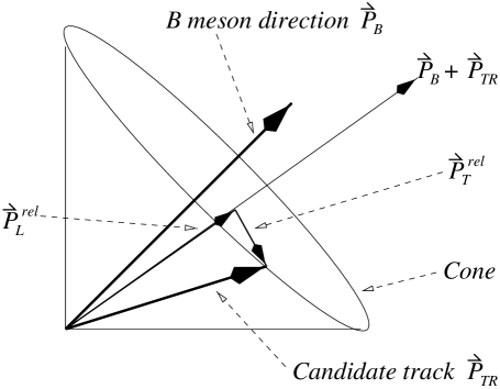
FIG. 2.: Schematic drawing of the momentum vectors determining $p_{T}^{rel}$ and $p_{L}^{rel}$ of an SST candidate.

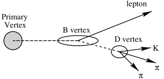
FIG. 3.: A typical $B\to\nu\ell D$ event topology, where a $B$ meson is produced at the event primary vertex, and decays after traveling a short distance into a lepton, a $D$ meson, and a neutrino (undetected, and not shown). The $D$ later decays into a kaon and one or more pions.

FIG. 4.: The mass distributions of the fully reconstructed $D$ candidates (solid histogram) for: $\ell^{+}D^{*-}$, $\overline{D}{{}^{0}}\to K^{+}\pi^{-}$ (upper left); $\ell^{+}D^{*-}$, $\overline{D}{{}^{0}}\to K^{+}\pi^{-}\pi^{+}\pi^{-}$ (upper right); $\ell^{+}D^{-}$, $D^{-}\to K^{+}\pi^{-}\pi^{-}$ (lower left) and $\ell^{+}\overline{D}{{}^{0}}$, $\overline{D}{{}^{0}}\to K^{+}\pi^{-}$(lower right). The dashed histograms are the distributions of the wrong-sign ($\ell^{\pm}K^{\mp}$) candidates. The number of signal events from the fit (solid curve) is indicated in each plot.

FIG. 5.: The distribution of $m(K\pi\pi_{*})-m(K\pi)$ for the signature $D^{*-}\to\overline{D}{{}^{0}}\pi_{*}^{-}$, $\overline{D}{{}^{0}}\to K^{+}\pi^{-}\pi^{0}$ ($\pi^{0}$ not reconstructed). The upper histogram is the distribution of the right-sign $\ell D$ candidates, and the lower histogram is for the wrong-sign combinations. The solid curve is the fit of the right-sign distribution, with the fitted background component shown by the upper dashed curve. This background shape is obtained from a fit (lower dashed curve) of the wrong-sign data.

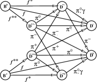
FIG. 6.: The state diagram for all possible $B\to\ell D^{(*)}X$ transitions. The $f$, $f^{*}$, and $f^{**}$ are semileptonic $B$ branching ratios to charm mesons.

FIG. 7.: The distribution of ${\cal K}\equiv p_{T}({\ell D})/p_{T}({B})$ (left), and ${\cal K}$ vs. $m(\ell D)$ (right) with a fit of a quadratic function, for the direct decay $\ell^{+}D^{*-}$, $\overline{D}{{}^{0}}\rightarrow K^{+}\pi^{-}$. The “error” bars in the ${\cal K}$ vs. $m(\ell D)$ plot represent the RMS spread of the ${\cal K}$-distribution in each bin, and not the error on the bin mean of ${\cal K}$.

FIG. 8.: The simulation for the direct chain $\ell D^{*-}$, with $\overline{D}{{}^{0}}\rightarrow K^{+}\pi^{-}$: $\Delta L_{\rm xy}(B)$ distribution, fitted with two Gaussians with relative fractions and RMS values listed (top left); $\Delta(1/\beta_{T}\gamma)/(1/\beta_{T}\gamma)$ distribution (top right); $\Delta ct$ distribution (bottom left); and the RMS of the $\Delta ct$ distribution as a function of $ct$ along with the linear fit for $\sigma^{ct}_{kd}(ct_{kd})$ (bottom right).

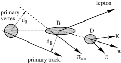
FIG. 9.: A schematic representation of a $B\rightarrow\nu\ell D^{**}$ decay. SST candidate tracks originate from the primary vertex, while the $\pi_{**}^{\pm}$ track originates from the $B$ decay vertex. The impact parameter of a track with respect to the primary vertex is $d_{0}$ while the impact parameter with respect to the $B$ vertex is given by $d_{B}$. When the $B$ vertex and the primary vertex are well separated, the $\pi_{**}^{\pm}$ track usually has a large $d_{0}$ and a small $d_{B}$. The converse is true for primary tracks.

FIG. 10.: Monte Carlo calculation of $\xi_{MC}$ as a function of corrected proper time, $ct^{0}_{kd}$, for decay signature $\ell^{+}D^{-}$: no $d_{0}/\sigma_{0}$ cut (top), and $d_{0}/\sigma_{0}<3.0$ (bottom).

FIG. 11.: Impact parameter distribution with respect to the $B$ vertex ($d_{B}/\sigma_{B}$) for the $\ell^{+}D^{-}$, $D^{-}\to K^{+}\pi^{-}\pi^{-}$ decay signature from the data (no $d_{0}/\sigma_{0}$ cut, $D$ mass sideband subtracted). Right-sign tags are shown by the solid points. Wrong-sign tags (open circles) are renormalized to model the right-sign continuum at large impact parameter significance, as described in the text. The right-sign excess near zero is due to the $\pi_{**}^{\pm}$ tags.

FIG. 12.: Measured asymmetries as a function of the corrected proper decay length $ct_{kd}$ for the decay signatures $\ell^{+}\overline{D}{{}^{0}}$ (dominated by $B^{+}$), $\ell^{+}D^{-}$, and the sum of all three $\ell^{+}D^{*-}$ (dominated by $B^{0}$). The three $\ell^{+}D^{*-}$ signatures are combined only for display purposes. The dashed line is the result of the fit.

FIG. 13.: The breakdown of the measured asymmetries of $\ell^{+}D^{*-}$ into the three $\ell^{+}D^{*-}$ decay signatures “$\ell^{+}D^{*-}$, $\overline{D}{{}^{0}}\to K^{+}\pi^{-}$”, “$\ell^{+}D^{*-}$, $\overline{D}{{}^{0}}\to K^{+}\pi^{-}\pi^{+}\pi^{-}$” and “$\ell^{+}D^{-}$, $D^{-}\to K^{+}\pi^{-}\pi^{-}$”. The result of the fit is overlaid.

FIG. 14.: Normalized mass distribution for $J/\psi K^{+}$ and $J/\psi K^{*0}$ candidates with reconstructed $ct>0$. The smooth curve is a fit from the full likelihood function of a Gaussian signal plus linear background parameterization.

FIG. 15.: Charge asymmetry ($\alpha$) dependence on the track’s $1/p_{T}$ (top) and number of primary vertices $n_{V}$ in the event (bottom) for: Same Side Tags (squares), SST candidate tracks (open circles), SST candidate tracks with $b$-vertex veto (solid circles), and tracks in a cone away from the $J/\psi$ direction (triangles). The solid curves are the results of least-squares fits of the asymmetry parameterization (see text) to the SST candidates with the $b$-vertex veto.

FIG. 16.: The $J/\psi K^{*0}$ lifetime distributions for the signal (top) and sideband (bottom) regions. Superimposed on the data are the likelihood fit results (solid line). In the signal region, the $B$ component is shown by the dashed line and the prompt plus long-lived background by the dotted line.

FIG. 17.: The mass sideband subtracted flavor-charge asymmetry as a function of the reconstructed $ct$ (points): left is $B^{+}\rightarrow J/\psi K^{+}$, and $B^{0}\rightarrow J/\psi K^{*0}$ is on the right. Superimposed on the data are the likelihood fit results (solid lines). The insets are scans through the log-likelihood functions as the dilutions are varied about the fit maxima. Also shown in the main plots are the results of simple $\chi^{2}$ fits to the points (dashed lines, partially obscured by the solid lines).

FIG. 18.: Number distributions of candidate tagging tracks in both $\ell D^{(*)}$ and $J/\psi K$ data (points) and simulation (shaded bands). The widths of the shaded bands are the statistical errors from the Monte Carlo sample size.

FIG. 19.: The $p_{T}$ distributions of the tag tracks in both $\ell D^{(*)}$ and $J/\psi K$ data (points) and simulation (shaded bands, width indicating the statistical error).

FIG. 20.: The $p_{T}^{rel}$ distributions of tag tracks in both $\ell D^{(*)}$ and $J/\psi K$ data (points) and simulation (shaded bands, width indicating the statistical error).

FIG. 21.: The extracted value of $\Delta m_{d}$ from the tagged $\ell D^{(*)}$ as a function of the tag $p_{T}$ threshold. Error bars are the naive statistical errors returned from the fit, and they are correlated with each other, as are the points themselves (see text).

FIG. 22.: Tagging dilution as a function of tag $p_{T}$ cut for $B^{0}$. Data are plotted with solid circles ($\ell D^{(*)}$) and triangles ($J/\psi K$), and the corresponding simulations are shown by the shaded bands (width indicates the statistical error). The various points and their errors are correlated with each other (see text).

FIG. 23.: Tagging dilution as a function of tag $p_{T}$ cut for $B^{+}$ data in the $\ell D^{(*)}$ (solid circles) and $J/\psi K$ (triangles) mode. The corresponding simulations are shown by the shaded bands (width indicates the statistical error). The various points and their errors are correlated with each other (see text).

FIG. 24.: Dilution as a function of the tag $p_{T}$ cut from Monte Carlo simulation for the $J/\psi K$ modes of $B^{0}$’s (solid square) and $B^{+}$’s (solid circle). When the tagging is restricted to prompt pions only, the neutral dilution becomes the open squares, and the charged the open circles.

FIG. 25.: Tagging efficiency as a function of the tag $p_{T}$ threshold for $\ell D^{(*)}$ (solid circles) and $J/\psi K$ (open triangles) data. The results from the simulation are shown by the shaded bands (width indicates the statistical uncertainty).

FIG. 26.: The sideband-subtracted $p_{T}(B)$ distributions for the (corrected) $\ell D^{(*)}$ (top) and $J/\psi K$ (bottom) samples. The charged and neutral $\ell D^{(*)}$ spectra are very similar, but the two $J/\psi K$ spectra are slightly different due to the different cuts on the kaon momenta.

FIG. 27.: Tagging dilution as a function of $B$ meson $p_{T}$ for charged (left) and neutral (right) mesons. The dilution measurements are plotted at the $p_{T}(B)$-weighted centroid of each bin, and the horizontal error bars span the width of the bin (arrows indicate that a bin is unbounded). The closed circles are the $\ell D^{(*)}$ data, and the open triangles are $J/\psi K$’s. The dashed curves are Monte Carlo calculations of the $p_{T}$ dependence, and the dotted lines mark the average dilution for the data points.

FIG. 28.: The $p_{T}$ distribution of tracks satisfying SST selection cuts except for the $p_{T}^{rel}$ requirement: average for $\ell D^{(*)}$ data (solid circles), default PYTHIA (open squares), and tuned PYTHIA (open circles).

FIG. 29.: The ratios of the $p_{T}(\ell)$ distributions of the data to the Monte Carlo simulation, for electrons (top) and muons (bottom), for the $\ell^{+}D^{-}$, $D^{-}\to K^{+}\pi^{-}\pi^{-}$ signature. The distributions are fit with the error function, where $p_{T}^{0}$ is the midpoint $p_{T}(\ell)$ and $\sigma_{p_{T}}$ the “width” of the turn-on. The overall normalizations are immaterial since the $\ell D^{(*)}$ analysis requires only relative efficiencies.

FIG. 30.: A comparison between the data and the single-$B$ Monte Carlo simulation for the decay signature $\ell^{+}D^{-}$, $D^{-}\to K^{+}\pi^{-}\pi^{-}$. The distributions compared are: $p_{T}$ of the lepton, $e$ and $\mu$ combined (top left), mass of the $\ell D^{-}$ system (top right), the $p_{T}$ of the $\ell D^{-}$ system (bottom left), and $p_{T}(\ell D^{-})$ after correcting for the missing neutrino (bottom right). Only the agreement in the corrected $p_{T}(\ell D^{-})$ distribution relates directly to the analysis.

FIG. 31.: Variation of $\gamma_{\phi}/\alpha_{\phi}$ versus $f_{1}$ and $f_{2}$ for $\alpha_{\phi}=2\%$ and nominal dilution ${\cal D}_{\phi}^{\prime}=16.6\%$. Note that (0,0) is the leftmost corner and (1,1) the rightmost, and that the function is not defined for the region $\Delta f<0$.

FIG. 32.: The distribution of $\zeta^{2}$ values obtained from $J/\psi K^{+}$ Monte Carlo samples equivalent to the data. A fit to the standard $\chi^{2}$ distribution is shown by the solid curve and yields 12.7 degrees of freedom. The vertical line indicates the $\zeta^{2}$ value obtained from the $J/\psi K^{+}$ data sample, and Monte Carlo samples with larger values of $\zeta^{2}$ are shaded.

REFERENCES

- [1] N. Cabibbo, Phys. Rev. Lett. 10, 531 (1963); M. Kobayashi and K. Maskawa, Prog. Theor. Phys. 49, 652 (1973).
- [2] UA1 Collaboration, C. Albajar et al., Phys. Lett. B 186, 247 (1987).
- [3] ARGUS Collaboration, H. Albrecht et al., Phys. Lett. B 192, 245 (1987).
- [4] For a recent review of experimental results on oscillations see O. Schneider, “Heavy Quark Spectroscopy, Oscillations, and Lifetime,” presented at the 18th International Symposium on Lepton-Photon Interactions, Hamburg, Germany, to appear in the proceedings.
- [5] HERA-B Collaboration, DESY-PRC 95/01, 1995; CLEO III Collaboration, Cornell CLNS 94/1277, 1994; BELLE Collaboration, KEK Report 3-1995, 1995; BaBar Collaboration, SLAC-R-95-457, 1995; D0 Collaboration, FERMILAB-Pub-96/357-E, 1996; CDFII Collaboration, FERMILAB-Pub-96/390-E, 1996.
- [6] CDF Collaboration, F. Abe et al., Phys. Rev. Lett. 80, 2057 (1998).
- [7] M. Gronau, A. Nippe, and J. Rosner, Phys. Rev. D 47, 1988 (1993); M. Gronau and J. L. Rosner, Phys. Rev. D 49, 254 (1994).
- [8] OPAL Collaboration, R. Akers et al., Z. Phys. C 66, 19 (1995).
- [9] ALEPH Collaboration, R. Barate et al., Phys. Lett. B 425, 215 (1998).
- [10] OPAL Collaboration, K. Ackerstaff et. al., CERN preprint CERN-EP/98-001.
- [11] CDF Collaboration, F. Abe et al., FERMILAB-Pub-98/189-E, submitted to Phys. Rev. Lett..
- [12] CDF Collaboration, F. Abe et al., Nucl. Instrum. Methods A 271, 387 (1988).
- [13] D. Amidei et al., Nucl. Instrum. Methods A 350, 73 (1994); P. Azzi et al., ibid. 360, 137 (1995).
- [14] CDF Collaboration, F. Abe et al., Phys. Rev. D 50, 2966 (1994).
- [15] CDF Collaboration, F. Abe et al., Phys. Rev. D 57, 5382 (1998).
- [16] ALEPH Collaboration, R. Buskulic et al., Phys. Lett. B 284, 177 (1992).
- [17] ALEPH Collaboration, R. Buskulic et al., Z. Phys. C 75, 397 (1997); OPAL Collaboration, K. Ackerstaff et al., ibid. 76, 401 (1997); ibid. 76, 417 (1997); DELPHI Collaboration, P. Abreu et al., ibid. 76, 579 (1997); L3 Collaboration, M. Acciarri, et al., CERN-EP/98-028, submitted to E. Phys. J. C.
- [18] CDF Collaboration, F. Abe et al., to be submitted to Phys. Rev. D.
- [19] OPAL Collaboration, R. Akers et al., Phys. Lett. B 327, 411 (1994).
- [20] R.D. Field and R.P. Feynman, Nucl. Phys. B 136, 1 (1978).
- [21] I. Dunietz and J.L. Rosner, Phys. Rev D 51, 2471 (1995).
- [22] Particle Data Group, R.M. Barnett et al., Phys. Rev. D 54, 1 (1996).
- [23] For a recent survey of production measurements, see C. J. Kreuter, “Measurements of ,” presented at the 2nd International Conference on B Physics and CP Violation, Honolulu, Hawaii, March 24-27, 1997, to appear in the proceedings.
- [24] D. Ebert, V.O. Galkin, and R.N. Faustov, Phys. Rev. D 57, 5663 (1998).
- [25] CLEO Collaboration, R. Fulton et al, Phys. Rev. D 43, 651 (1991).
- [26] N. Isgur, D. Scora, B. Grinstein, and M. Wise, Phys. Rev D 39, 799 (1989).
- [27] P. Maksimovic, Ph.D. dissertation, Massachusetts Institute of Technology, 1998 (unpublished).
- [28] CDF Collaboration, F. Abe et al., Phys. Rev. Lett. 76, 4462 (1996).
- [29] R.M. Barnett et al., Phys. Rev. D 54, 1 (1996), and 1997 off-year partial update for the 1998 edition available on the PDG WWW pages (URL: http://pdg.lbl.gov/).
- [30] CDF Collaboration, F. Abe et al., Phys. Rev. D 53, 3496 (1996).
- [31] CDF Collaboration, F. Abe et al., Phys. Rev. Lett. 72, 3456 (1994).
- [32] CDF Collaboration, F. Abe et al., Phys. Rev. Lett. 76, 2015 (1996); Phys. Rev. D 54, 6596 (1996).
- [33] CDF Collaboration, F. Abe et al., Phys. Rev. Lett. 75, 1451 (1995).
- [34] K. Kelley, Ph.D. dissertation, Massachusetts Institute of Technology, 1998 (unpublished).
- [35] P. Nason, S. Dawson, and R. K. Ellis, Nucl. Phys. B 327, 49 (1988).
- [36] A.D. Martin, W.J. Stirling, and P.G. Roberts, Phys. Rev. D 47, 867 (1993).
- [37] C. Peterson et al., Phys. Rev. D 27, 105 (1985).
- [38] P. Avery, K. Read, and G. Trahern, Cornell Internal Note CSN-212, 1985 (unpublished).
- [39] H.-U. Bengtsson and T. Sjöstrand, Computer Physics Commun. 46, 43 (1987); “PYTHIA 5.7 and JETSET 7.4: Physics and Manual,” by T. Sjöstrand (Lund U.) LU-TP-95-20, Aug 1995.
- [40] H.L. Lai et al., Phys. Rev. D 51, 4763 (1995).
- [41] D. Vucinic, Ph.D. dissertation, Massachusetts Institute of Technology, 1998 (unpublished).