Abstract

A search for Z boson decays to pairs of $b$-quark jets has been performed in the full dataset collected with the CDF detector at the Tevatron $p\bar{p}$ collider. After the selection of a pure sample of $b\bar{b}$ events by means of the identification of secondary vertices from $b$-quark decays, we have used two kinematic variables to further discriminate the electroweak $b\bar{b}$ production from QCD processes, and sought evidence for the Z decay in the dijet invariant mass distribution. An absolute background prediction allows the extraction of an excess of events inconsistent with the background predictions by $3.23\sigma$ but in good agreement with the amount and characteristics of the expected signal. We then fit the mass distribution with an unbinned likelihood technique, and obtain a $Z\to b\bar{b}$ signal amounting to $91\pm 30\pm 19$ events.

1 Introduction

Z decays to $b$-quark pairs are not exactly a unknown piece of Physics. Since 1992 the LEP experiments have detected several millions of them, and more have come from the polarized beams of the SLC. The process is thus very well understood; the Z is one of the best known particles, and there can be no surprise in the thereabouts. At a proton-antiproton collider this particular process has never been seen before, though. The UA2 collaboration published in 1987 an analysis of jet data where they could spot the combined signal of W and Z decays to dijet pairs, but the decay of the Z to $b$ quarks was not separated from the other hadronic decays.

The Z decay to $b$ quarks is the closest observable process to the expected decay of the Higgs boson, and —in view of the chances of a Higgs discovery in run 2 at the Tevatron— the understanding of the process, the knowledge of the expected mass resolution for a reconstructed decay, and the confidence with the kinematical tools that may help extracting it, are topics worth careful investigation. Moreover, a clean Z peak in a dijet mass distribution is useful for jet calibration, a relevant issue for the top quark mass measurement.

In the following we present a search for the $Z\to b\bar{b}$ process in $L=110pb^{-1}$ of $p\bar{p}$ collisions collected by CDF during the years 1992-1995. We will show that the signal can be extracted by means of a very stringent selection that allows a reduction of the background by four orders of magnitude, while retaining in the final dataset a handful of Z events.

This paper is organized as follows: in Section 2 we describe the CDF detector, the datasets used in the analysis, and the selection that leads to our final sample; in Section 3 the counting experiment is described, and the results are discussed; Section 4 deals with the unbinned likelihood fits to the mass distribution. In Section 5 we present our conclusions.

2 Data Selection

The CDF detector has been described in detail elsewhere. We only mention briefly here those detector components most relevant to this analysis. The silicon vertex detector (SVX) and the central tracking chamber (CTC) are immersed in a $1.4\,T$ axial field and provide the tracking and momentum measurement of charged particles. The SVX consists of four layers of silicon microstrip detectors and provides spatial measurement in the $r-\phi$ plane with a resolution of $15\,\mu m$. The CTC is a cylindrical drift chamber containing 84 layers grouped into 9 alternating superlayers of axial and stereo wires. The calorimeters, divided into electromagnetic and hadronic components, cover the pseudorapidity range $|\eta|<4.2$ and provide the jet energy measurement; they are segmented into projective towers subtending about $0.1\times 15^{o}$ in $\eta-\phi$ space. Central muon candidates are identified in two sets of muon chambers, located outside the calorimeters, as stubs extrapolating to charged tracks inside the solenoid. The data were collected by a three-level trigger system; the first two levels are provided by hardware modules, the third consists in software algorithms optimized for speed.

At the Tevatron the Z production cross section has been measured both in the $e^{+}e^{-}$ and in the $\mu^{+}\mu^{-}$ final states, and found to be $\sigma_{Z}\times BR(Z\rightarrow e^{+}e^{-})=0.235\,\pm\,0.003\,(stat.)\,\pm\,0.005\,(syst.)\,\pm\,0.020\,(lum.)\,nb$ and $\sigma_{Z}\times BR(Z\rightarrow\mu^{+}\mu^{-})=0.202\,\pm\,0.016\,(stat.)\,\pm\,0.020$ $(syst.)$ $\pm\,0.017\,(lum.)\,nb$. By scaling the $e^{+}e^{-}$ figures up to the b quark branching fraction one expects that about 110,000 Z decays to $b$-quark pairs have taken place at CDF during run 1, the cross section times branching ratio for the process resulting in $1.080\pm 0.029(stat.\oplus syst.)\pm 0.092(lum.)$ nanobarns.

The natural trigger for a $Z\to b\bar{b}$ signal would be a low energy jet trigger. However, the rate of jet production processes is too high to allow for a collection of all these events: the jet triggers are therefore prescaled, such that only a limited integrated luminosity is collected by them. The best dataset for a search of $Z\to b\bar{b}$ decays is instead the one collected by a trigger requiring the presence of a clean muon candidate: the $b$-quark jets produced in Z decays contain lots of low $P_{T}$ muons, originated in B hadron decays, sequential charmed hadron decays, or other processes in smaller amounts. The starting point of the search was therefore the sample of 5.5 million events featuring a $P_{T}>7.5\,GeV/c$ central muon candidate, corresponding to an integrated luminosity of $L=103\pm 7\,pb^{-1}$.

2.1 The Datasets

The initial dataset was cleaned up by requiring the muon candidate be also identified as a good muon by a standard offline filter. Jets were reconstructed by a fixed $R=0.7$ cone clustering algorithm, and two jets in each event were required to contain charged tracks forming a well identified secondary vertex (hereafter “SVX tag”, from the name of the silicon vertex detector). This selection reduced drastically the dataset, being satisfied by only 5,479 events. The selection discarded the non-heavy flavour component of the QCD background, and increased the signal/noise ratio by about two orders of magnitude.

We used the PYTHIA Monte Carlo to generate 1.7M $Z\to b\bar{b}$ decays that were subjected to a detector simulation, filtered by a trigger simulation, and passed through the same offline selection used for the real data. Using the predicted cross section for the searched process, the number of $Z\to b\bar{b}$ decays in the double SVX tagged dataset is expected to amount to $124\pm 14$ events.

As will be explained in the following, we have used real Z decays to electron-positron pairs collected during run 1 to better understand the behavior of initial state radiation in the Z production. These events were selected from high $E_{T}$ electron triggers by requiring the presence of a good quality central electron plus another electron candidate passing looser cuts. The dataset consists in more than six thousand events, and can be useful for kinematical studies, particularly when the variables one is interested in are difficult to model with Monte Carlo programs.

To study the contamination of other boson signals in our dataset we also generated 500,000 W boson decays to $c\bar{s}$ pairs and 500,000 Z decays to $c$-quark pairs with PYTHIA 5.7: in fact, these processes may give a contribution to the muon dataset, due to the presence of charm quarks in the final state. These events were subjected to the same treatment described for the $Z\to b\bar{b}$ data. Their contamination to the double SVX tags dataset was found to be totally negligible.

Sample	Run 1	$Z\to b\bar{b}$	Eff.	Events in
		PYTHIA		103 $pb^{-1}$
Initial		1,673,000		$(110\pm 12)10^{3}$
Trigger	5,414,755
2 SVX tags	5,479	1,867	21.3%	$124\pm 14$
$\Delta\Phi_{12}>3$	1,684	1,368	73.2%	$91\pm 11$
$\Sigma_{3}E_{T}<10$	588		(50.0%)	$(45\pm 21)$

Table 1: Number of events selected by each of the cuts described in the text for the experimental data and for the $Z\to b\bar{b}$ MC data, efficiency of each cut for the Z signal, and expected Z events in the total dataset. The signal size and the efficiency of the last cut ($\Sigma_{3}E_{T}<10\,GeV$) are estimated using $Z\to e^{+}e^{-}$ data.

2.2 Kinematical Tools

Even after the very restrictive selection of events with two SVX tags, the signal/noise ratio is too small to allow for a clear identification of the $Z\to b\bar{b}$ signal in the dijet mass distribution: other tools are needed to increase the discrimination of the electroweak production of $b$-quark jets from the strong interaction.

From a theoretical standpoint, one expects the two production processes to be different in many ways. The two initial state partons of the Z production have to be a quark-antiquark pair, and the process is time-like. On the contrary, in the QCD creation of a $b\bar{b}$ pair both a quark-antiquark and a gluon-gluon pair can give rise to a time-like direct production process, and also space-like diagrams may contribute. Many of the QCD processes are expected to result in a pair of outgoing partons with a flatter pseudorapidity distribution than those from the searched Z decay; but the double SVX tagging and the requirement of a central muon candidate in one of the two jets result in pseudorapidity distributions that are already very constrained and well peaked at zero, due to the acceptance of the SVX and the muon chambers.

If one examines the color structure of the diagrams one however notices a marked difference between $Z\rightarrow b\bar{b}$ and $g\rightarrow b\bar{b}$. In the QCD processes there is a color connection between the initial and the final state absent in the Z production. Furthermore, while both the initial and the final state of the Z production are in a color singlet configuration, the opposite is true for QCD tree level diagrams. These considerations alone may lead us to believe that QCD gives rise to processes with a higher color radiation accompanying the two $b$-quark jets; furthermore, the pattern of this radiation is different. In QCD processes, in fact, the color connection present at LO between the two final state partons and the initial state should give rise to a enhanced radiation flow in the planes containing each of the two leading jets and the z axis: color coherence prescribes the radiation from the incoming and outgoing partons to interfere constructively in these regions, while the color singlet produced in the Z decay will emit soft radiation mainly between the two leading jets.

Although no event-by-event discrimination appears possible by the use of variables that try to pinpoint the differences in the radiation pattern, two variables that deal inclusively with these features prove useful for our search. These are the azimuthal angle between the two $b$-quark jets, $\Delta\Phi_{12}$, and the sum of transverse energies of all the calorimeter clusters in the event beyond the two jets, $\Sigma_{3}E_{T}$: they both have some discriminating power between a high radiation process and the colorless production of a dijet system; but, while the first one is easy to simulate for Monte Carlo programs, being relatively independent from the modeling of the underlying event, the second is critically dependent on the detailed features of the initial state radiation mechanisms. For an homogeneous comparison one is therefore bound to use the experimental data to understand the behavior of the $\Sigma_{3}E_{T}$. The distribution of the SVX data (to be considered a pure background sample, due to the very low S/N ratio) in the plane of the two kinematic variables can thus be compared to that of experimental Z decays to $e^{+}e^{-}$ pairs, as shown in fig.1. The difference in the radiation flow for these two samples is evident.

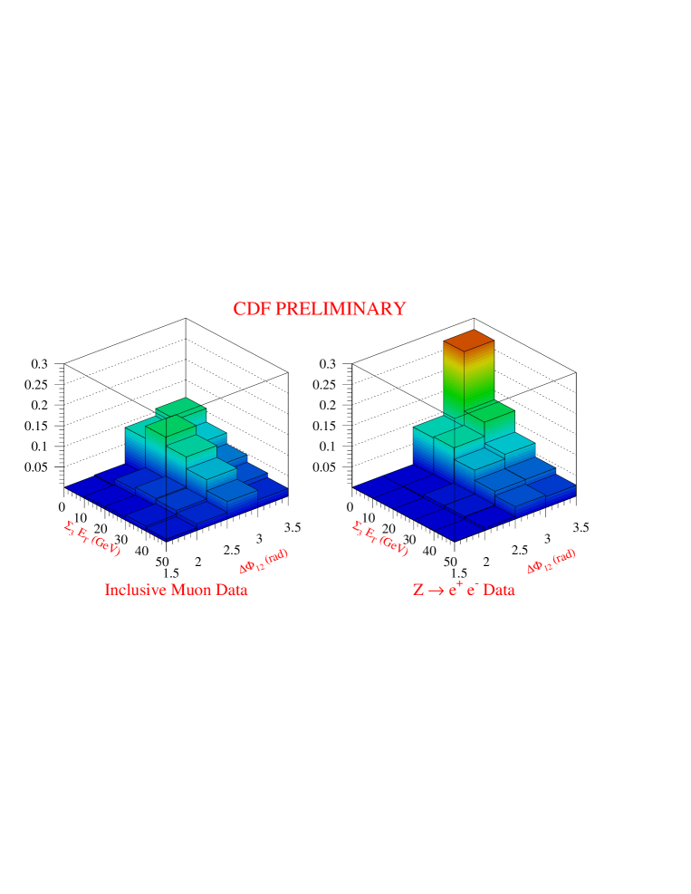
Figure 1: These plots prove the discriminating power between a QCD and a EWK process of the two kinematic variables we are selecting our data with. On the left is shown our SVX tagged data, on the right the $Z\to e^{+}e^{-}$ data. The two distributions are normalized to equal volume.

We therefore select our data by placing tight cuts on these two variables: we require the two leading jets to be separated in azimuth by at least three radians, and the additional clusterized $E_{T}$ be less than 10 GeV. These cuts will be shown to maximize the expected signal significance in Section 3.1, where all the ingredients necessary for the computation are presented.

3 The Counting Experiment

After the kinematic selection we expect the dataset to be still rich of background, with a S/N ratio as high as 1/6 for events with $M_{jj}\sim 90\,GeV/c^{2}$. Under such circumstances, the mass distribution can be used to demonstrate the presence of a signal only if the background shape is very well under control.

We use events where only one of the two leading jets carries a SVX tag as a background-enriched sample, and look for a signal as an excess of events in the double SVX data; to obtain a background estimate we rely on the observation that the probability of finding a secondary vertex in a jet is independent on the value of the kinematic variables we have selected our data with. We divide our data into four subsamples: events that fall in the kinematic region selected by our cuts ($\Delta\Phi_{12}>3$ radians, $\Sigma_{3}E_{T}<10\,GeV$, in the following referred to as the “Signal Zone”), and events that fail those requirements, from both the double tagged dataset —“(++)” in the following— and from events having only one tagged jet —hereafter “(+0)” events. We then define a tag probability as the ratio between (++) and (+0) events outside the Signal Zone, and extrapolate it inside, obtaining an absolute background prediction for the double tags in the Signal Zone:

$N^{++}_{exp,in}=N^{+0}_{obs,in}\times(N^{++}_{obs,out}/N^{+0}_{obs,out})$.

The procedure just outlined is carried out for each bin of invariant mass of the dijet system: by doing that, we obtain a tag probability as a function of the dijet mass, from which we evaluate an absolute background prediction $N^{++}_{exp,in}(M_{jj})$ that can be compared to the observed count in each bin of the mass distribution. An excess around $90\,GeV/c^{2}$ will be bias-free evidence for the signal, if away from there the excesses are compatible with zero.

3.1 The Choice of Cuts

In order to extract the highest possible significance from the excess of events in the dataset we have studied the expected signal significance as a function of the cuts on the kinematic variables used for the selection. Our definition of the significance for the present purpose is an approximation: we define it as $S=N_{signal}/(\sigma_{bgr}^{stat}\oplus\sigma_{bgr}^{syst}\oplus\sqrt{N_{tot}})$. The Monte Carlo is used to estimate $N_{signal}$ as a function of the cuts, while $N_{tot}$ is defined as the sum of $N_{signal}$ and the expected background, computed with the method described above. The statistical and systematic errors on the background prediction are added in quadrature to the Poisson fluctuation of the total expected number of events $N_{tot}$, giving a value of S per each choice of the cut on the variable studied. We are thus able to decide what are the best possible cuts on the two selection variables.

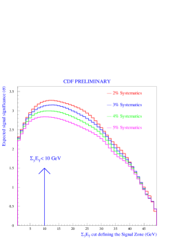
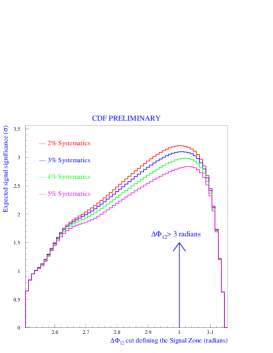
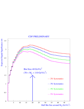
Figure 2: Maximization of the expected signal significance as a function of the cut on the kinematic variables. Left: choice of cut on $\Sigma_{3}E_{T}$; center: choice of the cut on $\Delta\Phi$; right: choice of the bin size. Four different possibilities for a systematic uncertainty in the background evaluation are considered.

As can be seen in fig.2, the chosen cuts on $\Delta\Phi$ and $\Sigma_{3}E_{T}$ do maximize the expected signal significance S, regardless of the systematic uncertainty attributed to the extrapolation of the tagging probability.

The same machinery can be used to decide the optimal binning in the dijet mass distribution for the counting experiment. The dijet mass is of course a very discriminant variable: by defining appropriately the width of the bin around $90\,GeV/c^{2}$ where we look for an excess of events over the background, we can again maximize the expected significance. Using the background prediction and the expected shape of the signal mass peak from Monte Carlo, we obtain significance curves that point to the best binning. The latter is chosen to be $40\,GeV/c^{2}$ wide, as shown in fig.2.

3.2 Results of the Counting Experiment

Having tuned cuts and binning to their most favorable values, we can perform the computation of the background and study the results. These are detailed in table 2.

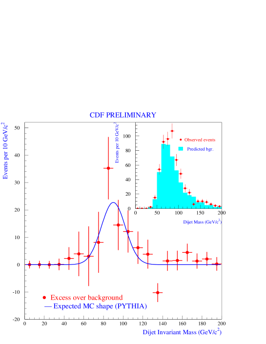
Figure 3: Results of the counting experiment with a $10\,GeV/c^{2}$ binning. The excess over background predictions is compared to the expected shape of a $Z\to b\bar{b}$ mass signal (PYTHIA). The inset shows the mass distribution of double tags (points with error bars) and the expected background (full histogram).

Mass Interval	Observed	Expected	Excess	Exp. Z
$0-30\,GeV/c^{2}$	0	$0.05\pm 0.09$	$-0.05\pm 1.40$
$30-70\,GeV/c^{2}$	163	$149.30\pm 6.13$	$13.70\pm 14.16$	$1.7\pm 0.8$
$70-110\,GeV/c^{2}$	318	$248.49\pm 8.95$	$69.51\pm 19.95$	$41.4\pm 18.8$
$110-150\,GeV/c^{2}$	66	$65.51\pm 4.68$	$0.49\pm 9.38$	$2.4\pm 1.1$
$150-190\,GeV/c^{2}$	29	$19.70\pm 2.59$	$9.30\pm 5.97$
$190-230\,GeV/c^{2}$	7	$7.06\pm 1.73$	$-0.06\pm 3.16$
$230-270\,GeV/c^{2}$	3	$2.24\pm 0.82$	$0.78\pm 2.38$
$270-310\,GeV/c^{2}$	1	$1.60\pm 0.95$	$-0.60\pm 2.00$
$310-350\,GeV/c^{2}$	0	$0.55\pm 0.98$	$-0.55\pm 1.71$
$350-390\,GeV/c^{2}$	1	$0.00\pm 0.00$	$1.00\pm 1.76$

Table 2: Results of the counting experiment.

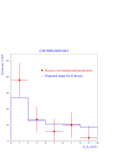
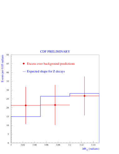
Figure 4: The excess observed in the $70\div 110\,GeV$ bin is distributed according to expectations in the $\Sigma_{3}E_{T}$ variable (left) and in the $\Delta\Phi$ variable (right).

The excess in the third bin is quite significant: using a conservative estimate of the systematic uncertainty in the extrapolation of the tag probability (a total of 4% is estimated from comparisons of observed and predicted events in signal-depleted samples) the prediction becomes $N_{exp}=248.49\pm 13.38$ events. The probability of a fluctuation of this number to the 318 observed events is 0.00061, equivalent to 3.23 standard deviations for a one-sided gaussian distribution.

The numbers quoted above are already compelling evidence for the presence of $Z\to b\bar{b}$ decays in our dataset. But we can use a smaller bin size to study the shape of the excess of events in the mass distribution: we then expect to see a gaussian peak at $90\,GeV/c^{2}$, with a r.m.s. of $12.3\,GeV/c^{2}$. The results of the counting experiment with this smaller bin size confirm the expectations: the excess fits very well to the expected signal shape (fig.3).

We have still another method to verify the assumption that we are observing a Z signal. In fact, the counting method allows a study of the behavior of the excess as a function of the same kinematic variables used for the data selection, that have been shown to have a distinctive shape for the electroweak process. To do that, we select (++) and (+0) events in the Signal Zone that fall in the interval $70<M_{jj}<110\,GeV/c^{2}$: as table 2 shows, we have an excess of $69.5\pm 20.0$ events there. We can then build the $\Sigma_{3}E_{T}$ and $\Delta\Phi$ distributions for the (++) events and compare them to the corresponding (+0) distributions scaled down by the tag probability $P_{90}=N^{++}_{obs,out}(70\div 110)/N^{+0}_{obs,out}(70\div 110)$. Indeed, the double SVX tags in excess are distributed in the two kinematic variables as expected for Z events, as can be seen in fig.4.

4 Unbinned Likelihood Fits to the Mass Distribution

Having established the presence of a $Z\to b\bar{b}$ signal in our dataset with a counting method, we can perform a two-component fit to the dijet mass distribution, and extract additional information from its shape.

We used a three-step procedure to fit the data. First of all, we obtained a background shape from a unbinned likelihood fit to a signal-depleted sample consisting in (+0) events falling outside of the Signal Zone. This sample is expected to be totally dominated by the QCD background, and can be successfully fit to the following simple functional form:
$P_{bgr}(M_{jj})=\frac{1}{\lambda}\cdot e^{-M_{jj}/\lambda}\otimes N(\mu,\sigma)$
where “$\otimes$” is the convolution operator, while $N(\mu,\sigma)$ is the Normal distribution. The fit is shown in the lower plot of fig.5.

The above form cannot be directly used as a background shape for double SVX events, since the probability of tagging a second jet is correlated to the invariant mass. To account for that, we obtained a tag probability curve $P(M_{jj})$ by performing a $\chi^{2}$ fit to the ratio of double and single SVX tags rejected by the kinematic cuts.

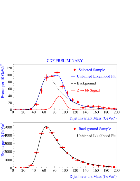
Figure 5: Top: results of the unbinned likelihood fit to the dijet mass distribution in the (++) sample; bottom: results of the unbinned likelihood fit to the dijet mass distribution of (+0) events rejected by the kinematic cuts.

The knowledge of the parameters of the two above fits allows us to write a two-component unbinned likelihood for the dijet mass distribution of the (++) sample, as follows:

$${\cal L}^{++} = P_{oisson}(\,N^{++},\,(n^{++}_{sig}+n^{++}_{bgr})\,)\cdot\prod_{i=1}^{N^{++}}\frac{n^{++}_{sig}\cdot P_{sig}(M_{i})+n^{++}_{bgr}\cdot P_{bgr}^{\prime}(M_{i})}{n^{++}_{sig}+n^{++}_{bgr}}$$

where: $N^{++}$ is the observed number of events in the (++) sample; $n^{++}_{sig}$ and $n^{++}_{bgr}$ are respectively the number of signal and background events in the (++) sample; $P_{bkg}^{\prime}(M)$ is the normalized background mass shape of the events in the (++) sample, obtained from the background fit to the single SVX data and the tag probability curve; and, finally, $P_{sig}(M)$ is a normalized gaussian describing the signal.

By maximizing $\log{\cal L}$ with respect to the number of signal and background events, and to the mass and width of the signal shape, but keeping frozen the background shape parameters and the tag probability curve parameters obtained previously, we obtained $n^{++}_{sig}=91\pm 30$ events, $M_{Z}=90.0\pm 2.4\,GeV/c^{2}$, and $\sigma_{Z}=9.4\pm 3.5\,GeV/c^{2}$; the fit results are shown in the upper plot of fig.5. The mass and width of the gaussian peak are in perfect agreement with Monte Carlo expectations ($M=90.0\,GeV/c^{2}$, $\sigma_{M}=12.3\,GeV/c^{2}$), while its normalization is in agreement to the excess obtained in Section 3.2 but is slightly larger than the Monte Carlo predictions ($N_{Z}=45.5\pm 20.7$ events). Although partially correlated to the results of the counting experiment, these numbers give additional qualitative informations on the behavior of the signal we have isolated.

Various studies of the possible systematic uncertainties of the fitting procedure have been performed. The systematic uncertainty due to the negligence of a signal contamination in the background sample was estimated to be $\pm 9$ events; the systematics due to the parametrization of the tag probability amount to $\pm 16$ events; and, finally, the systematic uncertainty due to the modeling of the background shape was showed to amount to $\pm 5$ events. Therefore the final result of the unbinned likelihood fit to the mass distribution is the following: $N_{Z}=91\pm 30(stat)\pm 19(syst)$ events.

5 Conclusions

We have searched 5.5 million inclusive muon events collected by CDF during run 1 for a $Z\to b\bar{b}$ signal. The very low signal/noise ratio at trigger level (less than $10^{-3}$) implies that a really strict selection is required in order to isolate a signal. We have designed an optimized selection for that purpose by making use of double SECVTX tagging plus some kinematic criteria suited to the discrimination of an electroweak production from the QCD background. By these means we select 588 events, 318 of whose have a reconstructed dijet invariant mass between 70 and 110 $GeV/c^{2}$, where the Z decay is expected to yield $41.4\pm 18.8$ events. By comparing the observed events with the expected background we find evidence of the signal, quantifiable in an excess of $69.5\pm 20.0$ events having a suggestive shape in the mass distribution. The excess corresponds to a $3.23\sigma$ fluctuation of the background, in the hypothesis of no signal. Finally, we have used a unbinned likelihood fit to the dijet mass distribution to obtain additional evidence of the presence of $91\pm 30$ (stat) $\pm 19$ (syst) $Z\to b\bar{b}$ decays in the signal sample.

We thank the Fermilab staff and the technical staffs of the participating institutions for their vital contributions. We also thank Michelangelo Mangano and Mike Seymour for many useful discussions. This work was supported by the U.S. Department of Energy and National Science Foundation; the Italian Istituto Nazionale di Fisica Nucleare; the Ministry of Education, Science and Culture of Japan; the Natural Sciences and Engineering Research Council of Canada; the National Science Council of the Republic of China; and the A.P.Sloan Foundation.