DESY-98-050

Abstract

The inclusive forward jet cross section in deep inelastic $e^{+}p$ scattering has been measured in the region of $x$–Bjorken,  $4.5\cdot 10^{-4}$  to  $4.5\cdot 10^{-2}$. This measurement is motivated by the search for effects of BFKL–like parton shower evolution. The cross section at hadron level as a function of $x$ is compared to cross sections predicted by various Monte Carlo models. An excess of forward jet production at small $x$ is observed, which is not reproduced by models based on DGLAP parton shower evolution. The Colour Dipole model describes the data reasonably well. Predictions of perturbative QCD calculations at the parton level based on BFKL and DGLAP parton evolution are discussed in the context of this measurement.

J. Breitweg, M. Derrick, D. Krakauer, S. Magill, D. Mikunas, B. Musgrave, J. Repond, R. Stanek, R.L. Talaga, R. Yoshida, H. Zhang
Argonne National Laboratory, Argonne, IL, USA ^p

M.C.K. Mattingly
Andrews University, Berrien Springs, MI, USA

F. Anselmo, P. Antonioli, G. Bari, M. Basile, L. Bellagamba, D. Boscherini, A. Bruni, G. Bruni, G. Cara Romeo, G. Castellini¹, L. Cifarelli², F. Cindolo, A. Contin, N. Coppola, M. Corradi, S. De Pasquale, P. Giusti, G. Iacobucci, G. Laurenti, G. Levi, A. Margotti, T. Massam, R. Nania, F. Palmonari, A. Pesci, A. Polini, G. Sartorelli, Y. Zamora Garcia³, A. Zichichi
University and INFN Bologna, Bologna, Italy ^f

C. Amelung, A. Bornheim, I. Brock, K. Coböken, J. Crittenden, R. Deffner, M. Eckert, M. Grothe⁴, H. Hartmann, K. Heinloth, L. Heinz, E. Hilger, H.-P. Jakob, A. Kappes, U.F. Katz, R. Kerger, E. Paul, M. Pfeiffer, J. Stamm⁵, H. Wieber
Physikalisches Institut der Universität Bonn, Bonn, Germany ^c

D.S. Bailey, S. Campbell-Robson, W.N. Cottingham, B. Foster, R. Hall-Wilton, G.P. Heath, H.F. Heath, J.D. McFall, D. Piccioni, D.G. Roff, R.J. Tapper
H.H. Wills Physics Laboratory, University of Bristol, Bristol, U.K. ^o

R. Ayad, M. Capua, L. Iannotti, M. Schioppa, G. Susinno
Calabria University, Physics Dept.and INFN, Cosenza, Italy ^f

J.Y. Kim, J.H. Lee, I.T. Lim, M.Y. Pac⁶
Chonnam National University, Kwangju, Korea ^h

A. Caldwell⁷, N. Cartiglia, Z. Jing, W. Liu, B. Mellado, J.A. Parsons, S. Ritz⁸, S. Sampson, F. Sciulli, P.B. Straub, Q. Zhu
Columbia University, Nevis Labs., Irvington on Hudson, N.Y., USA ^q

P. Borzemski, J. Chwastowski, A. Eskreys, J. Figiel, K. Klimek, M.B. Przybycień, L. Zawiejski
Inst. of Nuclear Physics, Cracow, Poland ^j

L. Adamczyk⁹, B. Bednarek, M. Bukowy, A.M. Czermak, K. Jeleń, D. Kisielewska, T. Kowalski,
M. Przybycień, E. Rulikowska-Zarȩbska, L. Suszycki, J. Zaja̧c
Faculty of Physics and Nuclear Techniques, Academy of Mining and Metallurgy, Cracow, Poland ^j

Z. Duliński, A. Kotański
Jagellonian Univ., Dept. of Physics, Cracow, Poland ^k

G. Abbiendi¹⁰, L.A.T. Bauerdick, U. Behrens, H. Beier¹¹, J.K. Bienlein, K. Desler, G. Drews, U. Fricke, I. Gialas¹², F. Goebel, P. Göttlicher, R. Graciani, T. Haas, W. Hain, D. Hasell¹³, K. Hebbel, K.F. Johnson¹⁴, M. Kasemann, W. Koch, U. Kötz, H. Kowalski, L. Lindemann, B. Löhr, J. Milewski, M. Milite, T. Monteiro¹⁵, J.S.T. Ng¹⁶, D. Notz, A. Pellegrino, F. Pelucchi, K. Piotrzkowski, M. Rohde, J. Roldán¹⁷, J.J. Ryan¹⁸, P.R.B. Saull, A.A. Savin, U. Schneekloth, O. Schwarzer, F. Selonke, S. Stonjek, B. Surrow¹⁹, E. Tassi, D. Westphal²⁰, G. Wolf, U. Wollmer, C. Youngman, W. Zeuner
Deutsches Elektronen-Synchrotron DESY, Hamburg, Germany

B.D. Burow, C. Coldewey, H.J. Grabosch, A. Meyer, S. Schlenstedt
DESY-IfH Zeuthen, Zeuthen, Germany

G. Barbagli, E. Gallo, P. Pelfer
University and INFN, Florence, Italy ^f

G. Maccarrone, L. Votano
INFN, Laboratori Nazionali di Frascati, Frascati, Italy ^f

A. Bamberger, S. Eisenhardt, P. Markun, H. Raach, T. Trefzger²¹, S. Wölfle
Fakultät für Physik der Universität Freiburg i.Br., Freiburg i.Br., Germany ^c

J.T. Bromley, N.H. Brook, P.J. Bussey, A.T. Doyle²², S.W. Lee, N. Macdonald, G.J. McCance, D.H. Saxon,
L.E. Sinclair, I.O. Skillicorn, E. Strickland, R. Waugh
Dept. of Physics and Astronomy, University of Glasgow, Glasgow, U.K. ^o

I. Bohnet, N. Gendner, U. Holm, A. Meyer-Larsen, H. Salehi, K. Wick
Hamburg University, I. Institute of Exp. Physics, Hamburg, Germany ^c

A. Garfagnini, L.K. Gladilin²³, D. Horstmann, D. Kçira²⁴, R. Klanner, E. Lohrmann, G. Poelz, W. Schott¹⁸, F. Zetsche
Hamburg University, II. Institute of Exp. Physics, Hamburg, Germany ^c

T.C. Bacon, I. Butterworth, J.E. Cole, G. Howell, L. Lamberti²⁵, K.R. Long, D.B. Miller, N. Pavel, A. Prinias²⁶, J.K. Sedgbeer, D. Sideris, R. Walker
Imperial College London, High Energy Nuclear Physics Group, London, U.K. ^o

U. Mallik, S.M. Wang, J.T. Wu
University of Iowa, Physics and Astronomy Dept., Iowa City, USA ^p

P. Cloth, D. Filges
Forschungszentrum Jülich, Institut für Kernphysik, Jülich, Germany

J.I. Fleck¹⁹, T. Ishii, M. Kuze, I. Suzuki²⁷, K. Tokushuku, S. Yamada, K. Yamauchi, Y. Yamazaki²⁸
Institute of Particle and Nuclear Studies, KEK, Tsukuba, Japan ^g

S.J. Hong, S.B. Lee, S.W. Nam²⁹, S.K. Park
Korea University, Seoul, Korea ^h

H. Lim, I.H. Park, D. Son
Kyungpook National University, Taegu, Korea ^h

F. Barreiro, J.P. Fernández, G. García, C. Glasman³⁰, J.M. Hernández, L. Hervás¹⁹, L. Labarga, M. Martínez, J. del Peso, J. Puga, J. Terrón, J.F. de Trocóniz
Univer. Autónoma Madrid, Depto de Física Teórica, Madrid, Spain ⁿ

F. Corriveau, D.S. Hanna, J. Hartmann, L.W. Hung, W.N. Murray, A. Ochs, M. Riveline, D.G. Stairs, M. St-Laurent, R. Ullmann
McGill University, Dept. of Physics, Montréal, Québec, Canada ${}^{a},$  ^b

T. Tsurugai
Meiji Gakuin University, Faculty of General Education, Yokohama, Japan

V. Bashkirov, B.A. Dolgoshein, A. Stifutkin
Moscow Engineering Physics Institute, Moscow, Russia ^l

G.L. Bashindzhagyan, P.F. Ermolov, Yu.A. Golubkov, L.A. Khein, N.A. Korotkova, I.A. Korzhavina, V.A. Kuzmin, O.Yu. Lukina, A.S. Proskuryakov, L.M. Shcheglova³¹, A.N. Solomin³¹, S.A. Zotkin
Moscow State University, Institute of Nuclear Physics, Moscow, Russia ^m

C. Bokel, M. Botje, N. Brümmer, J. Engelen, E. Koffeman, P. Kooijman, A. van Sighem, H. Tiecke, N. Tuning, W. Verkerke, J. Vossebeld, L. Wiggers, E. de Wolf
NIKHEF and University of Amsterdam, Amsterdam, Netherlands ⁱ

D. Acosta³², B. Bylsma, L.S. Durkin, J. Gilmore, C.M. Ginsburg, C.L. Kim, T.Y. Ling, P. Nylander, T.A. Romanowski³³
Ohio State University, Physics Department, Columbus, Ohio, USA ^p

H.E. Blaikley, R.J. Cashmore, A.M. Cooper-Sarkar, R.C.E. Devenish, J.K. Edmonds, J. Große-Knetter³⁴, N. Harnew, C. Nath, V.A. Noyes³⁵, A. Quadt, O. Ruske, J.R. Tickner²⁶, R. Walczak, D.S. Waters
Department of Physics, University of Oxford, Oxford, U.K. ^o

A. Bertolin, R. Brugnera, R. Carlin, F. Dal Corso, U. Dosselli, S. Limentani, M. Morandin, M. Posocco, L. Stanco, R. Stroili, C. Voci
Dipartimento di Fisica dell’ Università and INFN, Padova, Italy ^f

J. Bulmahn, B.Y. Oh, J.R. Okrasiński, W.S. Toothacker, J.J. Whitmore
Pennsylvania State University, Dept. of Physics, University Park, PA, USA ^q

Y. Iga
Polytechnic University, Sagamihara, Japan ^g

G. D’Agostini, G. Marini, A. Nigro, M. Raso
Dipartimento di Fisica, Univ. ’La Sapienza’ and INFN, Rome, Italy ${}^{f}~{}$

J.C. Hart, N.A. McCubbin, T.P. Shah
Rutherford Appleton Laboratory, Chilton, Didcot, Oxon, U.K. ^o

D. Epperson, C. Heusch, J.T. Rahn, H.F.-W. Sadrozinski, A. Seiden, R. Wichmann, D.C. Williams
University of California, Santa Cruz, CA, USA ^p

H. Abramowicz³⁶, G. Briskin, S. Dagan³⁷, S. Kananov³⁷, A. Levy³⁷
Raymond and Beverly Sackler Faculty of Exact Sciences, School of Physics, Tel-Aviv University,
Tel-Aviv, Israel ^e

T. Abe, T. Fusayasu, M. Inuzuka, K. Nagano, K. Umemori, T. Yamashita
Department of Physics, University of Tokyo, Tokyo, Japan ^g

R. Hamatsu, T. Hirose, K. Homma³⁸, S. Kitamura³⁹, T. Matsushita
Tokyo Metropolitan University, Dept. of Physics, Tokyo, Japan ^g

M. Arneodo²², R. Cirio, M. Costa, M.I. Ferrero, S. Maselli, V. Monaco, C. Peroni, M.C. Petrucci, M. Ruspa, R. Sacchi, A. Solano, A. Staiano
Università di Torino, Dipartimento di Fisica Sperimentale and INFN, Torino, Italy ^f

M. Dardo
II Faculty of Sciences, Torino University and INFN - Alessandria, Italy ^f

D.C. Bailey, C.-P. Fagerstroem, R. Galea, G.F. Hartner, K.K. Joo, G.M. Levman, J.F. Martin, R.S. Orr, S. Polenz, A. Sabetfakhri, D. Simmons, R.J. Teuscher¹⁹
University of Toronto, Dept. of Physics, Toronto, Ont., Canada ^a

J.M. Butterworth, C.D. Catterall, M.E. Hayes, T.W. Jones, J.B. Lane, R.L. Saunders, M.R. Sutton, M. Wing
University College London, Physics and Astronomy Dept., London, U.K. ^o

J. Ciborowski, G. Grzelak⁴⁰, M. Kasprzak, R.J. Nowak, J.M. Pawlak, R. Pawlak, B. Smalska,
T. Tymieniecka, A.K. Wróblewski, J.A. Zakrzewski, A.F. Żarnecki
Warsaw University, Institute of Experimental Physics, Warsaw, Poland ^j

M. Adamus
Institute for Nuclear Studies, Warsaw, Poland ^j

O. Deppe, Y. Eisenberg³⁷, D. Hochman, U. Karshon³⁷
Weizmann Institute, Department of Particle Physics, Rehovot, Israel ^d

W.F. Badgett, D. Chapin, R. Cross, S. Dasu, C. Foudas, R.J. Loveless, S. Mattingly, D.D. Reeder, W.H. Smith, A. Vaiciulis, M. Wodarczyk
University of Wisconsin, Dept. of Physics, Madison, WI, USA ^p

A. Deshpande, S. Dhawan, V.W. Hughes
Yale University, Department of Physics, New Haven, CT, USA ^p

S. Bhadra, W.R. Frisken, M. Khakzad, W.B. Schmidke
York University, Dept. of Physics, North York, Ont., Canada ^a

¹ also at IROE Florence, Italy
² now at Univ. of Salerno and INFN Napoli, Italy
³ supported by Worldlab, Lausanne, Switzerland
⁴ now at University of California, Santa Cruz, USA
⁵ now at C. Plath GmbH, Hamburg
⁶ now at Dongshin University, Naju, Korea
⁷ also at DESY
⁸ Alfred P. Sloan Foundation Fellow
⁹ supported by the Polish State Committee for Scientific Research, grant No. 2P03B14912
¹⁰ now at INFN Bologna
¹¹ now at Innosoft, Munich, Germany
¹² now at Univ. of Crete, Greece
¹³ now at Massachusetts Institute of Technology, Cambridge, MA, USA
¹⁴ visitor from Florida State University
¹⁵ supported by European Community Program PRAXIS XXI
¹⁶ now at DESY-Group FDET
¹⁷ now at IFIC, Valencia, Spain
¹⁸ now a self-employed consultant
¹⁹ now at CERN
²⁰ now at Bayer A.G., Leverkusen, Germany
²¹ now at ATLAS Collaboration, Univ. of Munich
²² also at DESY and Alexander von Humboldt Fellow at University of Hamburg
²³ on leave from MSU, supported by the GIF, contract I-0444-176.07/95
²⁴ supported by DAAD, Bonn
²⁵ supported by an EC fellowship
²⁶ PPARC Post-doctoral Fellow
²⁷ now at Osaka Univ., Osaka, Japan
²⁸ supported by JSPS Postdoctoral Fellowships for Research Abroad
²⁹ now at Wayne State University, Detroit
³⁰ supported by an EC fellowship number ERBFMBICT 972523
³¹ partially supported by the Foundation for German-Russian Collaboration DFG-RFBR
    (grant no. 436 RUS 113/248/3 and no. 436 RUS 113/248/2)
³² now at University of Florida, Gainesville, FL, USA
³³ now at Department of Energy, Washington
³⁴ supported by the Feodor Lynen Program of the Alexander von Humboldt foundation
³⁵ Glasstone Fellow
³⁶ an Alexander von Humboldt Fellow at University of Hamburg
³⁷ supported by a MINERVA Fellowship
³⁸ now at ICEPP, Univ. of Tokyo, Tokyo, Japan
³⁹ present address: Tokyo Metropolitan College of Allied Medical Sciences, Tokyo 116, Japan
⁴⁰ supported by the Polish State Committee for Scientific Research, grant No. 2P03B09308

a	supported by the Natural Sciences and Engineering Research Council of Canada (NSERC)
b	supported by the FCAR of Québec, Canada
c	supported by the German Federal Ministry for Education and Science, Research and Technology (BMBF), under contract numbers 057BN19P, 057FR19P, 057HH19P, 057HH29P
d	supported by the MINERVA Gesellschaft für Forschung GmbH, the German Israeli Foundation, the U.S.-Israel Binational Science Foundation, and by the Israel Ministry of Science
e	supported by the German-Israeli Foundation, the Israel Science Foundation, the U.S.-Israel Binational Science Foundation, and by the Israel Ministry of Science
f	supported by the Italian National Institute for Nuclear Physics (INFN)
g	supported by the Japanese Ministry of Education, Science and Culture (the Monbusho) and its grants for Scientific Research
h	supported by the Korean Ministry of Education and Korea Science and Engineering Foundation
i	supported by the Netherlands Foundation for Research on Matter (FOM)
j	supported by the Polish State Committee for Scientific Research, grant No. 115/E-343/SPUB/P03/002/97, 2P03B10512, 2P03B10612, 2P03B14212, 2P03B10412
k	supported by the Polish State Committee for Scientific Research (grant No. 2P03B08308) and Foundation for Polish-German Collaboration
l	partially supported by the German Federal Ministry for Education and Science, Research and Technology (BMBF)
m	supported by the Fund for Fundamental Research of Russian Ministry for Science and Education and by the German Federal Ministry for Education and Science, Research and Technology (BMBF)
n	supported by the Spanish Ministry of Education and Science through funds provided by CICYT
o	supported by the Particle Physics and Astronomy Research Council
p	supported by the US Department of Energy
q	supported by the US National Science Foundation

1 Introduction

One of the significant discoveries made at HERA was the steep rise of the proton structure function $F_{2}(x,Q^{2})$ in the region of small $x$–Bjorken ($\mbox{$x$}\leq 10^{-3}$) [1, 2]. Various attempts have been made to predict the behaviour of $F_{2}$. In one approach the $x$ dependence of $F_{2}$ is fitted at a fixed value of the scale $Q^{2}$ and then evolved taking into account $\ln Q^{2}$ terms according to the DGLAP [3] evolution equations [4, 5]. Different starting scales have been chosen for the evolution, down to values as small as $Q^{2}\approx 0.3\ {\rm GeV^{2}}$ [6]. In another approach the leading terms in $\ln(1/x)$ which appear together with $\ln Q^{2}$ terms in the evolution equations are resummed to yield the BFKL equation [7]. The appeal of the BFKL approach is the fact that it directly predicts the behaviour of $F_{2}$ as a function of $x$. The CCFM equation [8] interpolates between the two approaches and reproduces both the DGLAP and the BFKL behaviour in their respective ranges of validity. From the existing $F_{2}$ data it is not possible to determine unambiguously whether the BFKL mechanism plays a significant role in the HERA $x$-range.

Several exclusive measurements have been proposed in order to find evidence for BFKL effects [9, 10, 11, 12]. The method proposed by Mueller [13, 14] starts from the observation that the BFKL equation predicts a different ordering of the momenta in the parton cascade (see figure 1). The DGLAP equation predicts strong ordering of the parton transverse momenta $k_{T,i}$ while the BFKL equation relaxes this ordering but imposes strong ordering of the longitudinal momenta $x_{i}$:

DGLAP:    $x=x_{n}<x_{n-1}<...<x_{1}$,     $Q^{2}=k^{2}_{T,n}\gg k^{2}_{T,n-1}\gg...\gg k^{2}_{T,1};$

BFKL:        $x=x_{n}\ll x_{n-1}\ll...\ll x_{1}$,       No  ordering  in  $k_{T}$.

Thus the BFKL equation predicts additional contributions to the hadronic final state from partons with large transverse and longitudinal momenta, i.e. high transverse momentum partons going forward in the HERA frame. These partons may be resolved experimentally as jets and result in an enhancement of the forward jet cross section at small $x$ over NLO calculations and parton shower models based on DGLAP evolution.

The H1 collaboration has published results on the forward jet cross section [9] and the transverse energy flow in the forward direction [10] and found trends compatible with the expectations of BFKL dynamics.

In this paper we study forward jet production in a region which is expected to be sensitive to BFKL parton dynamics ($E^{2}_{T,Jet}\approx Q^{2}$). The comparison with standard QCD-inspired Monte Carlo models is also extended to the range where either $E^{2}_{T,Jet}\ll Q^{2}$ or $E^{2}_{T,Jet}\gg Q^{2}$. The measurement of the forward jet cross section is based on an order-of-magnitude increased statistics compared to [9]. Comparisons with different Monte Carlo models are presented and theoretical predictions are discussed in the context of this measurement.

Figure 1: Parton ladder diagram contributing to jet production in DIS. The emitted partons in the ladder extend from the bottom of the quark box down to the proton. The transverse momenta, $k_{T,i}$, and the longitudinal momentum fractions, $x_{i}$, with respect to the momenta of the incoming proton, evolve along the ladder.

2 Experimental Setup and Trigger

In 1995 HERA operated with 174 colliding bunches of $E_{p}=$ 820 GeV protons and $E_{e}=$ 27.5 GeV positrons. Additionally 21 unpaired bunches of protons or positrons circulated to determine the beam–related background. The integrated luminosity taken in 1995 and used in this analysis is 6.36 pb^-1. A detailed description of the ZEUS detector can be found in [15]. In the following the detector components relevant for this analysis are briefly described.

The central tracking detector (CTD) is surrounded by a superconducting solenoid. Outside the solenoid is the uranium calorimeter [16], which is divided in three parts: forward (FCAL), barrel (BCAL) and rear (RCAL) covering the polar angle region of 2.6^o to 176.2^o. The calorimeter covers 99.9% of the solid angle, with holes of 20$\times$12 cm² in the centre of the rear and of $20\times 20$ cm² in the forward calorimeter to accommodate the beam pipe. Each of the calorimeter parts is subdivided into towers which are segmented longitudinally into electromagnetic (EMC) and hadronic (HAC) sections. These sections are further divided into cells, each of which is read out by two photomultipliers. The size of the central FCAL EMC (HAC) cells is $20\times 5$ cm² ($20\times 20$ cm²). From test beam data, energy resolutions of $\sigma_{E}/E=0.18/\sqrt{E}$ for positrons and $\sigma_{E}/E=0.35/\sqrt{E}$ for hadrons ($E$ in GeV) were obtained. The effects of uranium noise are minimised by discarding cells in the EMC or in the HAC sections if they have energy deposits of less than 60 MeV or 110 MeV, respectively.

A three–level trigger is used to select events online [15]. The selection criteria are similar to those for the measurement of $F_{2}$ [17]. For $Q^{2}$ greater than 10 GeV² the trigger efficiency for DIS events is above 97%. About $7\cdot 10^{6}$ events survive our trigger requirements.

3 Event Selection

Events are selected offline if the $Z$-component of their primary vertex reconstructed from tracks in the CTD lies within $\pm 50$ cm around the nominal vertex. A positron candidate with an energy $E_{e^{\prime}}$ above 10 GeV is required. Candidates hitting the RCAL front face within a box of $X\times Y=13\times 8~{}{\rm cm}^{2}$ around the beam line are rejected because of possible energy loss into the beam hole. The fractional energy transfer $y_{JB}$ by the virtual photon in the proton rest frame, calculated from the hadronic energy [18] in the calorimeter, is required to be $y_{JB}>0.1$. This assures sufficient hadronic energy in the calorimeter to measure the event parameters with good accuracy. The $y_{el}$, i.e. the $y$ parameter calculated from the positron energy and angle, is required to be below 0.8. This rejects photoproduction events with low energy fake positron candidates in the FCAL. The quantity $E-P_{Z}=\Sigma_{i}E_{i}(1-\cos\theta_{i})$ is required to lie between 35 and 65 GeV. This requirement also removes photoproduction background. Here $E_{i}$ and $\theta_{i}$ are the energies and the polar angles of the calorimeter cells. For DIS events in an ideal detector $E-P_{Z}$ is equal to twice the energy of the incoming positron. Events within the $x$ range of  $4.5\cdot 10^{-4}$  to  $4.5\cdot 10^{-2}$  are finally selected for the cross section measurement.

4 Monte Carlo Simulation

Monte Carlo event simulation was used to correct the measured distributions for detector acceptance and smearing effects. The detector simulation is based on the GEANT [19] program and incorporates our understanding of the detector and of the trigger. Events were generated with DJANGO 6.24 [20], which interfaces HERACLES 4.5.2 [21] to either the Colour Dipole model [22] as implemented in ARIADNE 4.08 [23] or to LEPTO 6.5 [24]. HERACLES includes photon and $Z^{0}$ exchanges and first order electroweak radiative corrections. All samples were generated with the proton structure function CTEQ4D [4] which describes the measured $F_{2}$ structure function [1].

The Colour Dipole model treats gluons emitted from quark–antiquark pairs as radiation from a colour dipole between two partons. This results in partons which are not ordered in their transverse momenta $k_{T}$. Thus ARIADNE is frequently referred to as “BFKL–like” although it does not make explicit use of the BFKL equation. The hadronisation in ARIADNE is based on the LUND string model as implemented in JETSET [25].

Another event sample was generated with the MEPS option of DJANGO, as implemented into LEPTO. Here the hard interaction is taken from the first order matrix element, but the higher orders are simulated by a parton shower based on the DGLAP equation. Thus this sample provides a $k_{T}$–ordered parton shower. The hadronisation of the partons is done in the same way as in ARIADNE, i.e. via JETSET. In addition to the hard processes, this version of LEPTO has non–perturbative effects implemented, so–called Soft Colour Interaction (SCI), which affect the investigated phase space region.

A third sample was generated with HERWIG 5.9 [26], which like LEPTO has a parton shower evolution based on DGLAP. However, there are some differences with respect to LEPTO, such as the implementation of colour coherence effects or gluon splitting in the cluster hadronisation of the fragmentation phase.

A fourth sample was generated at hadron level only with the Linked Dipole Chain model option (LDC, version 1.0) [27] of ARIADNE, which uses its own structure functions. The parametrisation of “set A” was used, which fits data from H1 and ZEUS. In this model the parton shower evolution is based on a reformulation [28] of the CCFM approach [8] which approximates the BFKL prediction at low $x$ and the DGLAP prediction in the high-$x$ limit.

All Monte Carlo events were generated with the default settings of the input parameters. The first three samples were passed through the full trigger and detector simulation and were analysed in the same way as the real data. Additional Monte Carlo samples were generated but not passed through the detector simulation in order to study the parton and hadron–level properties of the jets.

The effect of initial and final state QED radiation was studied by generating ARIADNE events with and without QED corrections. After applying all event and jet selection cuts the jet cross sections as a function of $x$ with and without QED corrections agree within 5%. We conclude that QED radiation effects are small and ignore them in the following.

5 Jet Finding Algorithm and Jet Selection

5.1 Jet Algorithm

The analysis is performed with the cone jet algorithm according to the Snowmass convention [29]. The algorithm is applied to calorimeter cells in the laboratory frame where the cells assigned to the scattered positron are excluded.

The algorithm maximises the transverse energy flow $E_{T}$ through a cone of radius $R=\sqrt{(\triangle\eta)^{2}+(\triangle\phi)^{2}}$. Here $R=1$ is used and $\triangle\eta$ and $\triangle\phi$ are the differences of pseudorapidities and azimuthal angles with respect to the jet direction. The axis of the jet is calculated as the transverse energy weighted mean of the pseudorapidity and azimuth of all calorimeter cells belonging to the jet. The transverse energy threshold for the seed cells in the algorithm is set to 0.5 GeV. Two jets are merged if the overlapping energy exceeds 75% of the total energy of the jet with the lower energy. Otherwise two jets are formed and the common cells are assigned to the nearest jet. The massless option, where $E_{T,Jet}=p_{T,Jet}$, is used.

5.2 Jet Selection Criteria

In order to account for the energy loss of the jets in the inactive material of the detector an energy correction procedure is applied both to the total and transverse energies of the jets. The correction functions were obtained from the Monte Carlo simulations and are parametrised as a function of the total and transverse jet energy.

After the energy correction, several cuts are applied to select forward jets. The pseudorapidity of the jet is restricted to $\eta_{Jet}<2.6$ (equivalent to $\theta_{Jet}>8.5^{\circ}$). In this region the jets are well reconstructed. The transverse energy of the jets, measured with respect to the direction of the incoming proton, is above 5 GeV. The scaled longitudinal momentum $x_{Jet}=p_{Z,Jet}/820~{}{\rm GeV}$ is above 0.036. This selects forward jets. The cut $0.5<E^{2}_{T,Jet}/Q^{2}<2$, together with the $x_{Jet}$ cut, selects the phase space region where BFKL effects are expected. In about 2% of the events, two forward jets survive our selection cuts. In these cases the jet with the largest $x_{Jet}$ is selected. All these cuts restrict the $Q^{2}$ of the selected events to values above $\approx 12$ GeV².

For events at large values of $x$, the jet coming from the scattered quark can go sufficiently far forward to survive our cuts. In order to reject these events, all found jets are boosted into the Breit frame [30]. The boost is calculated from the four–momentum of the virtual photon, which is taken as the difference between the incoming and the outgoing four–momenta of the positron. Those jets which are in the current region of the Breit frame, i.e. which have negative $Z$–momentum, are rejected. This only affects the two highest $x$ bins where up to 50% of the jets are rejected.

All the selection criteria relevant for the phase space region which defines our cross section measurement are listed in table 1. A total of 2918 events with forward jets survive these cuts.

$E_{e^{\prime}}>10$ GeV

$y>0.1$

$\eta_{Jet}<2.6$

$E_{T,Jet}>5$ GeV

$x_{Jet}>0.036$

$0.5<E^{2}_{T,Jet}/Q^{2}<2$

$p_{Z,Jet}(Breit)>0$

$4.5\cdot 10^{-4}<x<4.5\cdot 10^{-2}$

Table 1: Selected phase space region for the cross section measurement.

6 Comparison of Data and Monte Carlo Distributions

Before applying the jet selection criteria, the data and the Monte Carlo predictions are compared. They agree well in absolute normalisation and in shape.

After applying the jet selection cuts the uncorrected differential cross sections as a function of the event related quantities $Q^{2}$, $E_{e^{\prime}}$, $y_{JB}$ and $E-P_{Z}$ are compared in figure 2. ARIADNE describes the measured distributions reasonably well while the LEPTO and HERWIG cross sections are too small.

In figure 3 we show uncorrected detector–level cross sections as a function of the jet–related quantities $E_{T,Jet}$, $x_{Jet}$, $\eta_{Jet}$ and $E_{T,Jet}^{2}/Q^{2}$. The distributions are compared to the predictions of the various Monte Carlo models. All selection criteria are applied except the one for the displayed variable. The data in the shaded areas are excluded from the final cross section measurement. ARIADNE describes the data in the first three distributions both in shape and in absolute value over the entire range. HERWIG and LEPTO underestimate the cross section significantly and also disagree in shape.

The distribution in figure 3d) can be subdivided into three regions. For small $E^{2}_{T,Jet}/Q^{2}$, i.e. the classical DIS regime, all three models agree with the data. Here $Q^{2}$ is large compared to $E^{2}_{T,Jet}$ and the DGLAP–based Monte Carlo models are expected to describe the data. In the unshaded region, which is selected for this analysis, only ARIADNE reproduces the data. HERWIG and LEPTO predict much smaller cross sections. In this area we expect significant contributions from BFKL–based parton showers. For higher values of $E^{2}_{T,Jet}/Q^{2}$ no model agrees with the

Figure 2: Uncorrected detector–level cross sections after the event and jet selection cuts as a function of a) $Q^{2}$, b) $E_{e^{\prime}}$, c) $y$, d) $E-P_{Z}$. Data are shown as points, ARIADNE as the full histogram, LEPTO as the dashed histogram and HERWIG as the dotted histogram. Only statistical errors are shown.

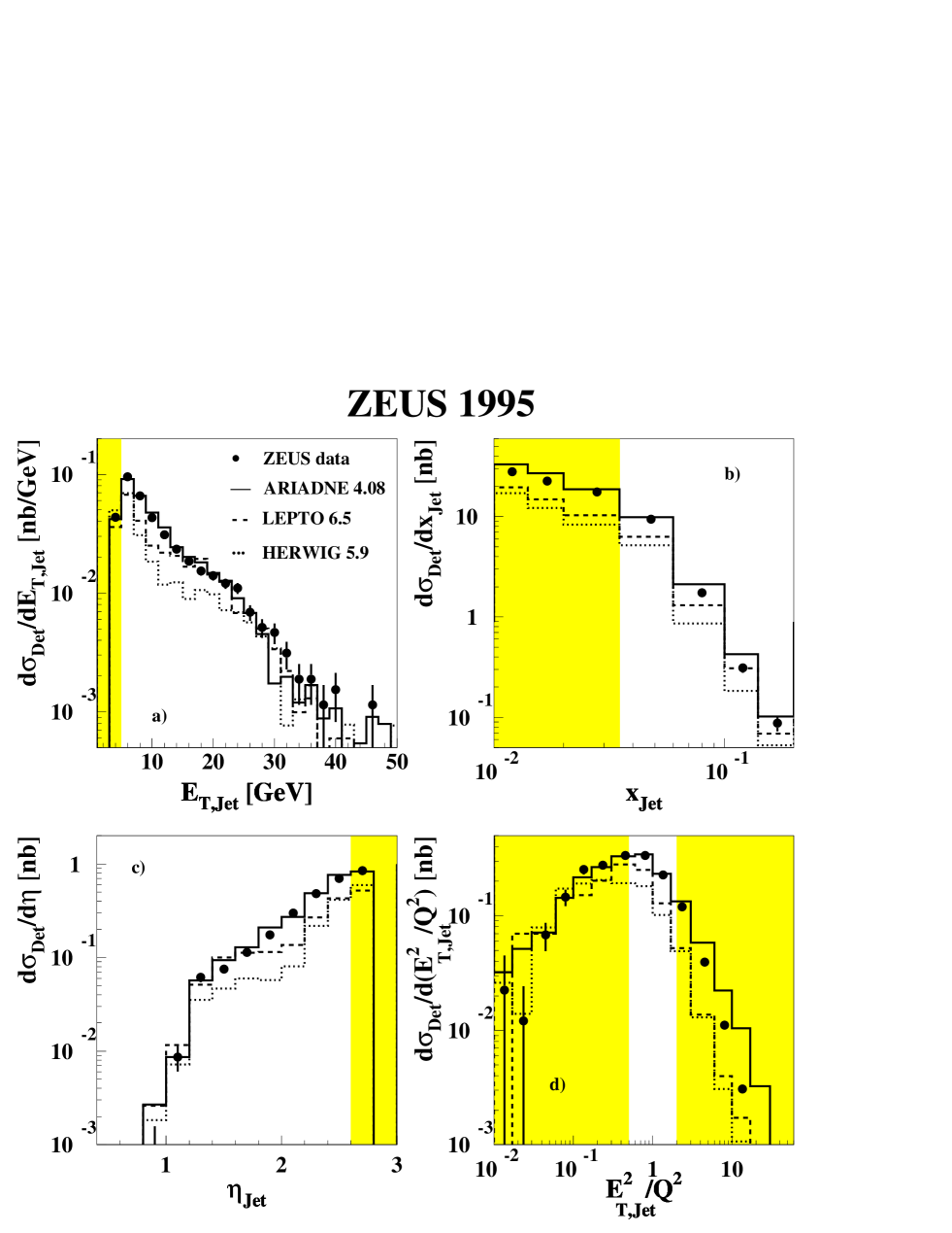
Figure 3: Uncorrected detector–level cross sections are shown as a function of a) $E_{T,Jet}$, b) $x_{Jet}$, c) $\eta_{Jet}$, d) $E^{2}_{T,Jet}/Q^{2}$. All event and jet selection cuts are applied (see text) apart from the cut on the displayed variable. Data are shown as points, ARIADNE as the full histogram, LEPTO as the dashed histogram and HERWIG as the dotted histogram. The data in the shaded areas are excluded from the final cross section measurement. Only statistical errors are shown.

data. The cross section of ARIADNE is too large, whereas those of LEPTO and HERWIG are too small. In this regime the hard scale is no longer given by the invariant mass squared, $Q^{2}$, of the virtual photon, but by the $E^{2}_{T}$ of the jets.

A study of energy flows similar to [31] has been performed in order to investigate whether jets in the forward region of the detector still have a pronounced signature and how the beam hole and the proton remnant affect the selected jets.

In figure 4 we show the transverse energy flow with respect to the forward jet axis averaged over all selected events as a function of $\triangle\phi$ and $\triangle\eta$, the difference in azimuth and pseudorapidity of the cells with respect to the jet direction. The grey bars indicate energy deposits in cells which are attributed to the forward jet. The black bars indicate the contributions from those cells situated in the towers directly surrounding the forward beam hole. As can be seen, some black bars also belong to the jet. The white bars indicate energy deposits which belong neither to the jet nor to the cells surrounding the FCAL beam hole. For increasing $\eta_{Jet}$ the black band–like structure in the forward direction of the jet, which we attribute to the proton remnant, becomes more and more prominent. For $\eta_{Jet}>2.6$ the selected jets pick up significant contributions from the proton remnant in their tails. Studies of the reconstruction accuracy of the angle and of the energy of the jets also show a degradation at $\eta_{Jet}$ values above 2.6 (not shown). Therefore, we require $\eta_{Jet}<2.6$ for this analysis.

In figure 5 we show the integrated jet shape $\Psi_{Det}(r)$, i.e. the relative amount of transverse energy deposited inside a cone of radius $r<R$ with respect to the jet axis. This function is defined as

$$\Psi_{Det}(r)=\frac{1}{N_{Jets}}\sum_{Jets}\frac{E_{T}(r)}{E_{T}(r=R)},$$

where $E_{T}(r)$ is the sum of the transverse energies of all cells of a given jet within a radius $r$ with respect to the jet axis. ARIADNE describes the distribution well for all values of $E_{T,Jet}$. LEPTO generates broader jets than observed in the data. The jets are more collimated as $E_{T,Jet}$ increases. A similar level of agreement between the data and the Monte Carlo events is found when bins of $\eta_{Jet}$ instead of $E_{T,Jet}$ are investigated (not shown).

7 Jet Finding Efficiencies and Purities

A detailed study of the jet reconstruction quality was performed in order to find acceptable cuts for the analysis.

ARIADNE was used for the study of the efficiencies and purities of the jet reconstruction and of the acceptance correction since it describes the data best in shape and absolute rate. The efficiency $\epsilon$ and purity $p$ of the jet finding are determined as a function of $x$ and are defined by:

$$\epsilon={{Number~{}of~{}jets^{det\oplus had}}\over{Number~{}of~{}jets^{had}}},\hskip 85.35826ptp={{Number~{}of~{}jets^{det\oplus had}}\over{Number~{}of~{}jets^{det}}}.$$

The indices det and had correspond to jets found at the detector or hadron level, respectively. Hadron–level jets are defined as jets found by the jet algorithm when applied to the stable hadrons from the event generator. The symbol  det$\oplus$had  means that the jet has to be found at both  levels in the  relevant  variable  range and in the same $x$–bin. The det jets  are  those

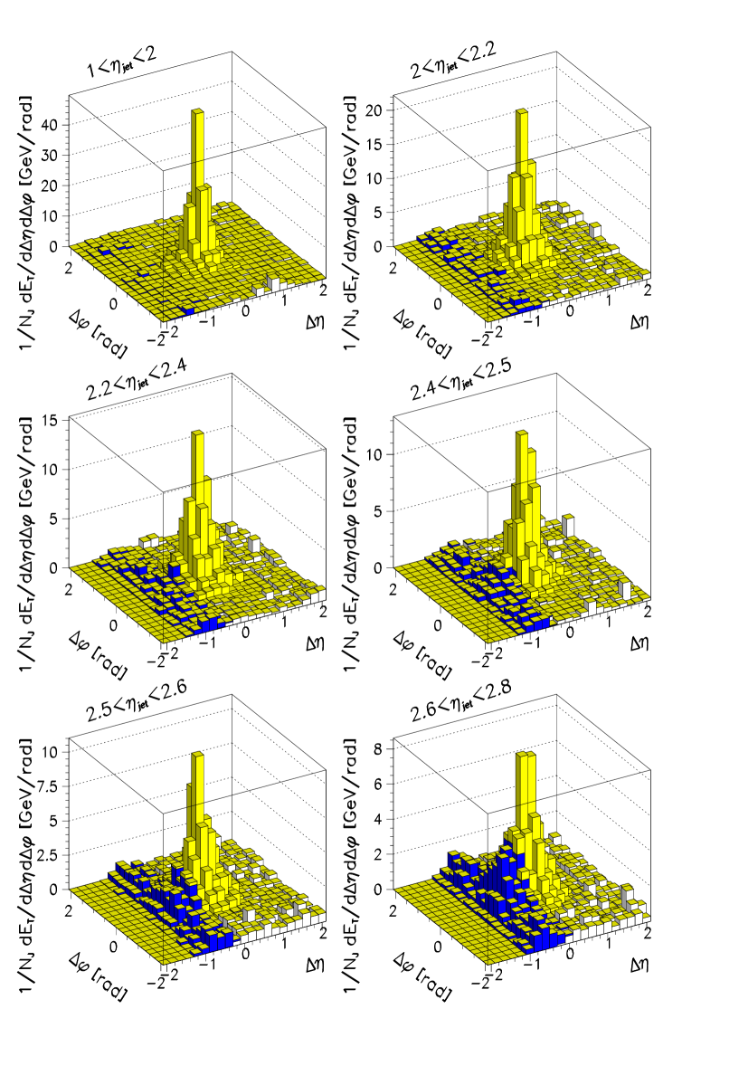
Figure 4: The transverse energy flow around the forward jet axis averaged over all selected forward jets for various $\eta_{Jet}$ regions. Grey bars indicate the transverse energy in the calorimeter cells attributed to the jet, black bars correspond to the transverse energy in the cells around the beam hole, and white bars correspond to the transverse energy elsewhere in the calorimeter.

Figure 5: Uncorrected integrated jet shapes in intervals of $E_{T,Jet}$ which are chosen to contain approximately equal numbers of jets. Data are shown as dots. Predictions from ARIADNE (LEPTO) are shown as full (dashed) lines. All event and jet selection cuts are applied. The statistical errors are negligible compared to the size of the dots.

surviving all the event and jet selection criteria and the had jets have to survive only those cuts which define the phase space region for which the final forward jet cross section is given, see table 1. Figure 6 shows as a function of $x$ the efficiencies $\epsilon$, purities $p$ and correction factors $c=p/\epsilon$ for the acceptance correction from detector to hadron level. The $x$ bins are chosen such that the bin width is at least 2–3 times the $x$ resolution and the statistical errors are below 20%. The values for $\epsilon$ and $p$ lie between 20% and 50%, while those of the correction factors are between 1.0 and 1.5. The drop in $\epsilon$ and $p$ for $\mbox{$x$}>10^{-2}$ is due to the degraded resolution of $x$ in this region of $x$. The small overall values of $\epsilon$ and $p$ are a result of the jet selection cuts and of the finite resolutions of the jet variables. The resolutions are: $\Delta E_{T,Jet}/E_{T,Jet}\simeq 10$%, $\Delta\eta_{Jet}\simeq 0.1$, $\Delta x_{Jet}/x_{Jet}\simeq 11$%, and $\Delta(E^{2}_{T,Jet}/Q^{2})~{}/~{}(E^{2}_{T,Jet}/Q^{2})\simeq 25$%. The latter has the largest effect on $\epsilon$ and $p$. When the cut on $E^{2}_{T,Jet}/Q^{2}$ is dropped the efficiencies and purities increase by about a factor of two. The measured detector–level rates are multiplied bin–by–bin using the correction factor $c$ in order to obtain the hadron–level distributions. In an independent analysis the acceptance correction was evaluated using the Bayes unfolding method [32]. This method

Figure 6: a) Purity, b) efficiency and c) correction factors for the correction of the detector–level jet cross section to the hadron–level jet cross section as a function of $x$.

takes migration effects between the bins properly into account and is a cross check of the reliability of the bin–by–bin acceptance correction. The extracted forward jet cross sections agree well between the two methods.

The analysis was also repeated using the $k_{T}$ clustering algorithm [33] in the Breit frame with $Q^{2}$ as scale and a resolution parameter $y_{cut}=0.5$. With these settings the algorithm creates a large number of jets at the detector level, which do not have a corresponding jet at the hadron or parton level. A change of the $y_{cut}$–parameter does not improve this situation. Purities and efficiencies in the lowest $x$ bins are therefore very small, around 5% and 15%, respectively. Nevertheless, the $k_{T}$ analysis leads to conclusions consistent with those drawn in this paper.

8 Comparison of DGLAP and BFKL Approaches

Perturbative QCD predicts the dynamics of the parton evolution. The conventional method to solve the parton evolution equations is the DGLAP approach [3], which resums leading order (LO) terms proportional to $(\ln Q^{2})^{n}$. This results in a parton cascade strongly ordered in transverse momentum $k_{T}$, where the parton with the highest transverse momentum appears at the lepton vertex of the chain. The longitudinal momenta $x_{Jet}$ decrease towards the photon vertex.

Next–to–leading–order (NLO) calculations, i.e. full second order matrix element calculations including first order virtual corrections, where parton densities are incorporated according to the DGLAP scheme, are available in three program packages MEPJET, DISENT and DISASTER$++$ [34, 35, 36]. The programs use different techniques to calculate cross sections but nevertheless agree reasonably well in their predictions [36]. These NLO calculations are not available in full Monte Carlo event simulations. They are purely parton–level calculations, delivering parton four momenta which can be analysed, such that the parton level cross sections can be evaluated using different jet algorithms and recombination schemes.

The BFKL approach [7] of the parton evolution resums terms proportional to $(\ln 1/\mbox{$x$})^{n}$, which become dominant over the $\ln Q^{2}$ terms at small $x$. This approach is expected to be valid in the high energy limit, where the total available energy, $W$, is large with respect to any other hard scale, $E_{T,Jet}$ or $Q$, in DIS. The first term of this resummation is second order in the strong coupling constant $\alpha_{s}$ and is therefore included in the next–to–leading order tree–level diagrams in DGLAP–based calculations, e.g. in MEPJET. In figure 1 this term corresponds to exactly one parton rung in the gluon ladder between the quark box and the proton. In the following it will be referred to as the BFKL 1^st term. Since the present approach is only leading $\ln 1/x$, the parton emissions are strongly ordered in $x_{Jet}$. Recent calculations of next–to–leading $\ln 1/\mbox{$x$}$ terms in the BFKL kernel [37] predict large negative corrections due to a weakening of the strong ordering in $x_{Jet}$ which are expected to reduce the cross section significantly.

The present BFKL calculations do not allow the implementation of a jet algorithm. Therefore this calculation can only be regarded as approximate, since the measured jet rates depend on the jet algorithm and on their resolution parameters, scales and recombination schemes. For example, in our selected phase space region MEPJET yields cross sections for the cone and the $k_{T}$ algorithm with their particular choice of parameters which differ by up to 15%.

In figure 7 we compare the differential forward jet cross section prediction from MEPJET to the BFKL 1^st term and to the leading order (LO) BFKL calculation. We have applied the cone algorithm within MEPJET, the same algorithm as used for the data. The renormalisation scale in the MEPJET program is varied between 0.25 $k^{2}_{T}$ and 2 $k^{2}_{T}$ to study the scale dependence of the parton–level cross section. Here $k_{T}$ is the scalar sum of the transverse momenta of the jets in the Breit frame. The result changes by $\sim$30% in the two small–$x$ bins and less than 10% in the other bins. This is indicated by the shaded band in figure 7.

The MEPJET NLO and the BFKL 1^st–term calculations are similar and predict a much smaller cross section than the LO BFKL calculation, which shows a steep rise towards smaller values of $x$.

Also shown are the parton–level cross sections from LEPTO, HERWIG, ARIADNE and from LDC. Both the MEPS–based LEPTO and HERWIG models show reasonable agreement with the MEPJET calculations, whereas ARIADNE exhibits a stronger increase of the cross section for small $x$. The LDC model is well below the ARIADNE predictions. For increasing $x$ all models and calculations converge.

For a direct comparison of the data to the theoretical calculations, the measurements need to be evaluated at the parton level, where partons are defined in the Monte Carlo at the stage after the last branching of the parton shower and before the hadronisation. The size of the corrections from hadron to parton level is studied using the Monte Carlo simulation programs and are displayed in figure 8. ARIADNE yields factors close to unity and shows no dependence as a function of $x$. LEPTO and HERWIG show large corrections for small $x$ values. This is expected, because these DGLAP based models, which have LO matrix element calculations implemented, can only produce a significant number of forward jets due to hadronisation effects and detector smearing. The LDC corrections are intermediate to LEPTO/HERWIG and ARIADNE. As shown above LEPTO and HERWIG also fail to describe the cross section both in absolute size and in shape. Furthermore, the relation between the parton level in parton shower Monte Carlo programs and partons in exact NLO calculations is not obvious. Therefore we refrain from quoting measurements corrected to the parton level.

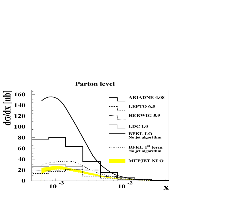
Figure 7: Parton–level predictions for forward jet cross sections as a function of $x$. The LO BFKL calculation is indicated by the full curve and the BFKL 1^st–term calculation as the dashed–dotted curve. The shaded band gives the range of results obtained with MEPJET using a renormalisation scale between $0.25~{}k^{2}_{T}$ and $2.0~{}k^{2}_{T}$. The predictions from ARIADNE (full histogram), LEPTO (dashed histogram), HERWIG (dotted histogram) and LDC (thin full histogram) are also shown.

Figure 8: Correction factors corresponding to the ratio of the parton level to the hadron–level forward jet cross section as a function of $x$. The factors for ARIADNE are shown as full circles, for LDC as open circles, for HERWIG as open rectangles and for LEPTO as full rectangles.

9 Systematic Studies

We have studied the effects of the variation of several selection cuts and reconstruction uncertainties on the final cross section. Figure 9 shows the percentage change of the final cross section in each $x$ interval for the major contributions to the overall systematic error.

Change of the $E-P_{Z}$ cut from $>$ 35 to $>$ 40 GeV
This tests the amount of photoproduction background in the sample and changes the result by less than 6%.

Alignment uncertainty between the CTD and the FCAL
The primary event vertex is determined from tracks in the CTD. In order to account for an alignment uncertainty between CTD and FCAL, the $Z$–position of the vertex is shifted by $\pm$ 0.4 cm. This affects mostly parameters calculated for the scattered positron and related quantities like $x$, $Q^{2}$ and the boost to the Breit frame. The uncertainty from this effect is around 5%, except in the highest $x$ bin where it reaches 14%. Here, due to the misreconstruction of the kinematic variables the current jet may be reconstructed sufficiently far forward to survive our selection cuts.

Jet energy scale uncertainty
The energy of the jets is scaled by $\pm$5% in the Monte Carlo, reflecting a global uncertainty of the hadronic energy scale in the forward region of the FCAL. The result changes by less than 15%.

Electromagnetic energy scale uncertainty of the calorimeter
The energy of the scattered positrons in the RCAL is scaled by $\pm$1% in the Monte Carlo corresponding to the global uncertainty of the electromagnetic energy scale in the calorimeter. The result changes typically by less than 5%.

Uncertainty from jet selection criteria
A possible mismatch between the distributions of jet variables in the data and in the Monte Carlo is tested by a variation of the cut values by about one sigma of their resolution followed by the determination of the cross sections at the nominal value of the cuts at the hadron level. The tested cuts are: the minimum $E_{T,Jet}$ (changed from 5 GeV to 4.5 and 5.5 GeV), the minimum $x_{Jet}$ (changed from 0.036 to 0.042 and to 0.030), the maximum $\eta_{Jet}$ (changed from 2.6 to 2.7 and 2.5), and the minimum and maximum $E^{2}_{T}/Q^{2}$ (changed from 0.5 to 0.6 and 0.4 or from 2 to 2.4 and 1.6, respectively). All these effects are at the level of a few percent, except in the lowest $x$ bin, where they add up to 18%. They are combined (i.e. added in quadrature separately for the positive and negative changes) and shown as “jet cuts” in figure 9.

Acceptance correction with LEPTO
The full acceptance correction is performed with LEPTO instead of ARIADNE. Since the $E^{2}_{T,Jet}/Q^{2}$ distribution of LEPTO differs substantially from the measured one, the LEPTO events were reweighted to reproduce the observed $E^{2}_{T,Jet}/Q^{2}$ distribution. This test changes the cross section by less than 15%, except in the lowest and the highest $x$ bins, where it increases the result by +20% and +60%, respectively.

Further checks included the variation of the accepted ranges of the primary event vertex ($\pm 40$ cm or $\pm 60$ cm instead of $\pm 50$ cm), a change of the region for the rejected scattered positrons within a box of $13\times 8$ cm² or $14\times 14$ cm² around the RCAL beam pipe, and a variation of the $y_{el}$ cut from $<$ 0.8 to $<$ 0.95. The effect on the cross section is negligible. A global uncertainty of 1.5% coming from the luminosity measurement is not included.

Figure 9: Percentage change of the forward jet cross section due to various systematic checks in the different $x$ bins. The vertical lines indicate the statistical errors in each interval. Empty bins contain values outside the displayed range (see text).

10 Hadron–Level Forward Jet Cross Section

In figure 10 we present the hadron–level forward jet cross section. The numerical values are given in table 2. ARIADNE describes the hadron–level forward jet cross section reasonably well, apart from the small–$x$ region, where it is slightly below the data. LEPTO and HERWIG, as well as LDC, predict significantly smaller cross sections. Switching off the Soft Colour Interaction in LEPTO decreases the cross section in the smallest $x$ bin by about 50%, but does not affect the large–$x$ region. Increasing the probability of Soft Colour Interaction from the default value of 50% to 100% does not increase the cross section.

The region of large $x$ can be seen more clearly in figure 10b). The data, ARIADNE and LEPTO converge at larger $x$. In this region, where $x_{Jet}$ approaches $x$, the phase space for parton emission is small. Therefore, the cross section is expected to be largely independent of the parton shower mechanism. On the other hand, HERWIG and LDC stay below the data.

The excess of forward jets at small $x$ observed in the data with respect to LEPTO and HERWIG may be interpreted as an indication of hard physics not implemented in present models of DGLAP–based parton evolution. However, the current implementation of BFKL–type physics, as exemplified by the LDC model, still underestimates the measured forward jet cross section.

$x$ range		$\frac{\displaystyle d\sigma}{\displaystyle dx}\pm{\rm stat.}\pm{\rm syst.}~{}[{\rm nb}]$	syst. ($E_{CAL}$ scale) $[$nb$]$
$4.5\cdot 10^{-4}$ –	$8.0\cdot 10^{-4}$	$114\pm 9.7^{\,+\,29}_{\,-\,15}$	($-5.9,~{}+18$)
$8.0\cdot 10^{-4}$ –	$1.4\cdot 10^{-3}$	$96.2\pm 6.5^{\,+\,8.2}_{\,-\,8.2}$	($-8.1,~{}+7.8$)
$1.4\cdot 10^{-3}$ –	$2.5\cdot 10^{-3}$	$77.8\pm 4.7^{\,+\,5.2}_{\,-\,6.9}$	($-4.2,~{}+7.0$)
$2.5\cdot 10^{-3}$ –	$4.5\cdot 10^{-3}$	$34.4\pm 2.2^{\,+\,3.8}_{\,-\,1.9}$	($-2.1,~{}+2.6$)
$4.5\cdot 10^{-3}$ –	$8.0\cdot 10^{-3}$	$14.1\pm 1.0^{\,+\,2.5}_{\,-\,1.2}$	($-1.2,~{}+1.3$)
$8.0\cdot 10^{-3}$ –	$1.4\cdot 10^{-2}$	$6.53\pm 0.54^{\,+\,0.1}_{\,-\,0.7}$	($-0.7,~{}+0.2$)
$1.4\cdot 10^{-2}$ –	$2.5\cdot 10^{-2}$	$2.65\pm 0.25^{\,+\,0.3}_{\,-\,0.3}$	($-0.03,~{}+0.2$)
$2.5\cdot 10^{-2}$ –	$4.5\cdot 10^{-2}$	$0.65\pm 0.09^{\,+\,0.1}_{\,-\,0.4}$	($-0.00,~{}+0.05$)

Table 2: Forward jet cross sections and their errors for the kinematic region given in table 1. The last column shows the correlated systematic error due to the energy scale uncertainty of the calorimeter, which is not included in the central column. It corresponds to the shaded band in figure 10.

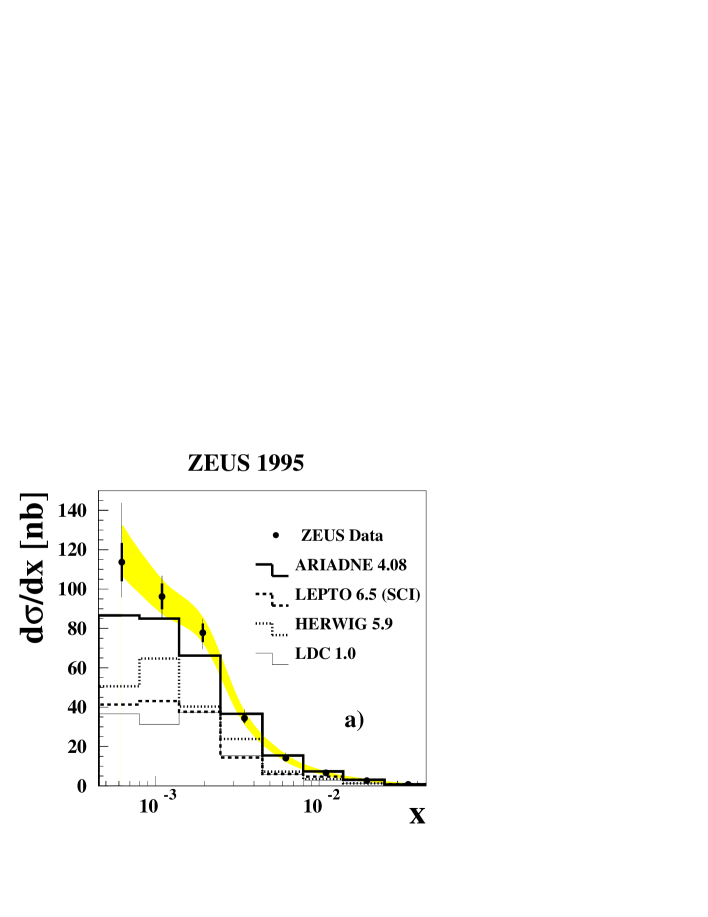
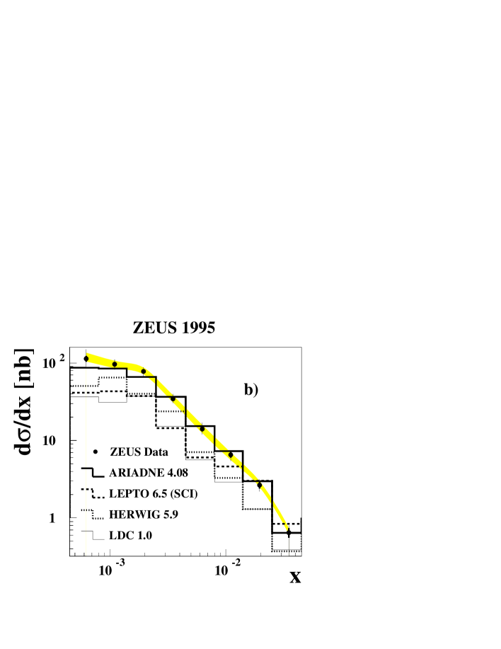
Figure 10: Forward jet cross section at hadron level as a function of $x$ in the kinematic region $\eta_{Jet}$$<2.6$, $x_{Jet}$$>0.036$, $0.5<E^{2}_{T,Jet}/Q^{2}<2$, $E_{T,Jet}>5$ GeV, $E_{e^{\prime}}>10$ GeV, $y>0.1$. a) Linear scale, b) logarithmic scale. Statistical errors are shown as thick error bars, and statistical and systematic errors added in quadrature as thin error bars. The errors due to the uncertainty of the jet energy scale are shown as the shaded band.

11 Summary and Conclusions

An investigation of forward jet production including a comparison to various Monte Carlo models has been performed. Three regions are identified in the $E^{2}_{T,Jet}/Q^{2}$ distribution: i) the standard DGLAP region with $E^{2}_{T,Jet}\ll Q^{2}$, where all Monte Carlo models are in agreement with the data; ii) the region of phase space where BFKL dynamics is expected to contribute significantly with $E^{2}_{T,Jet}\approx Q^{2}$, where only the Colour Dipole model describes the data well, and iii) the region with $E^{2}_{T,Jet}\gg Q^{2}$, where none of the models reproduces the data.

The forward jet cross section at hadron level is measured in the region ii) where $E^{2}_{T,Jet}\approx Q^{2}$. The cross section is compared to the predictions of several models: ARIADNE, which includes one of the main features of the BFKL–based phenomenology, that is the absence of the strong ordering in the transverse momenta in the parton shower; LDC, which is based on the CCFM approach and which smoothly interpolates between the BFKL and the DGLAP predictions in their range of validity; and, LEPTO and HERWIG, which are based on leading order DGLAP parton evolution. The measured cross section is reasonably well described by ARIADNE while LEPTO, HERWIG and LDC predict cross sections that are too low at small $x$. The excess of forward jets at small $x$ observed in the data with respect to LEPTO and HERWIG may be interpreted as an indication of hard physics not implemented in present models of DGLAP–based parton evolution. However, the current implementation of BFKL–type physics, as exemplified by the LDC model, still underestimates the measured forward jet cross section.

References

-
[1]
ZEUS Collab., M. Derrick et al.,
Phys. Lett. B 316 (1993) 412;
ZEUS Collab., M. Derrick et al., Z. Phys. C 65 (1995) 379;
ZEUS Collab., M. Derrick et al., Z. Phys. C 69 (1996) 607. -
[2]
H1 Collab., I. Abt et al.,
Nucl. Phys. B 407 (1993) 515;
H1 Collab., T. Ahmed et al., Nucl. Phys. B 439 (1995) 471. -
[3]
V.N. Gribov and L.N. Lipatov,
Sov. J. Nucl. Phys. 15 (1972) 438 and 675;
Yu.L. Dokshitzer, Sov. Phys. JETP 46 (1977) 641;
G. Altarelli and G. Parisi, Nucl. Phys. B 126 (1977) 298. - [4] H.L. Lai et al., Phys. Rev. D 55 (1997) 1280.
- [5] A.D. Martin, R.G. Roberts and W.J. Stirling, Phys. Lett. B 387 (1996) 419.
-
[6]
M. Glück, E. Reya and A. Vogt,
Phys. Lett. B 306 (1993);
M. Glück, E. Reya and A. Vogt, Z. Phys. C 67 (1995) 433. -
[7]
E.A. Kuraev, L.N. Lipatov and V.S. Fadin,
Sov. Phys. JETP 45 (1977) 199;
Ya.Ya. Balitzki and L.N. Lipatov, Sov. J. Nucl. Phys. 28 (1978) 822. -
[8]
M. Ciafaloni, Nucl. Phys. B 296 (1988) 49;
S. Catani, F. Fiorani and G. Marchesini, Phys. Lett. B 234 (1990) 339 and Nucl. Phys. B 336 (1990) 18;
G. Marchesini, Nucl. Phys. B 445 (1995) 49. - [9] H1 Collab., S. Aid et al., Phys. Lett. B 356 (1995) 118.
- [10] H1 Collab., I. Abt et al., Z. Phys. C 63 (1994) 377.
-
[11]
J. Bartels et al.,
Phys. Lett. B384 (1996) 300;
J. Bartels, V. del Duca and M. Wüsthoff, Z. Phys. C 76 (1997) 75. - [12] H1 Collab., C. Adloff et al., Nucl. Phys. B 485 (1997) 3.
-
[13]
A.H. Mueller,
Nucl. Phys. B (Proc. Suppl) 18 C (1990) 125;
A.H. Mueller, Journ. of Phys. G 17, (1991) 1443. -
[14]
J. Bartels, A. De Roeck et M. Loewe,
Z. Phys. C 54 (1992) 635;
J. Kwiecinski, A.D. Martin and P.J. Sutton, Phys. Lett. B 287 (1992) 254; Phys. Rev. D 46 (1992) 921;
W.K. Tang, Phys. Lett. B 278 (1992) 363;
J. Bartels, M. Besançon, A. De Roeck and J. Kurzhoefer; Proceedings of the HERA Workshop 1992 (eds. W. Buchmüller and G. Ingelman), p. 203. -
[15]
ZEUS Collab., M. Derrick et al.,
Phys. Lett. B 303 (1993) 183;
The ZEUS Detector, A Status Report 1993, DESY 1993. -
[16]
M. Derrick et al.,
Nucl. Inst. Meth. A 309 (1991) 77;
A. Andresen et al., Nucl. Inst. Meth. A 309 (1991) 101;
A. Bernstein et al., Nucl. Inst. Meth. A 336 (1993) 23. - [17] ZEUS Collab., M. Derrick et al., Z. Phys. C 72 (1996) 399.
- [18] F. Jacquet and A. Blondel, Proc. of the Study for an Facility for Europe, ed. U. Amaldi, DESY 79/48 (1979) 391.
-
[19]
R. Brun et al.,
GEANT program manual, CERN program library (1992);
Geant 3.13, CERN DD/EE/84-1 (1987). - [20] DJANGO 6.24, K. Charchula, G.A. Schuler and H. Spiesberger, Comp. Phys. Comm. 81 (1994) 381.
- [21] HERACLES 4.5.2, A. Kwiatkowski, H.–J. Möhring and H. Spiesberger, Comp. Phys. Comm. 69 (1992) 155.
- [22] B. Andersson et al., Z. Phys. C 43 (1989) 625.
-
[23]
ARIADNE 4.08, L. Lönnblad,
Comp. Phys. Comm. 71 (1992) 15;
L. Lönnblad, Z. Phys. C 65 (1995) 285. - [24] LEPTO 6.5, G. Ingelman, A. Edin and J. Rathsman, Comp. Phys. Comm. 101 (1997) 108.
- [25] JETSET 7.4, T. Sjöstrand, Comp. Phys. Comm. 82 (1994) 74.
- [26] HERWIG 5.9, G. Marchesini et al., Comp. Phys. Comm. 67 (1992) 465.
-
[27]
B. Andersson, G. Gustafson and J. Samuelsson,
Nucl. Phys. B 463 (1996) 217;
B. Andersson, G. Gustafson, H. Kharraziha and J. Samuelsson, Z. Phys. C 71 (1996) 613;
H. Kharraziha and L. Lönnblad, LU–TP 97–21, hep-ph/9709424. - [28] B. Andersson, G. Gustafson, J. Jannelson, Nucl. Phys. B 463 (1996) 217.
-
[29]
J. Huth et al.,
Proc. of the 1990 DPF Summer Study on High Energy Physics,
Snowmass, Colorado edited by E.L. Berger (World Scientific, Singapore, 1992)
p. 134;
CDF Collab., F. Abe et al., Phys. Rev. D 45 (1992) 1448;
ZEUS Collab., J. Breitweg et al., Eur. Phys. J. C 2 (1998) 61. - [30] ZEUS Collab., M. Derrick et al., Z. Phys. C 67 (1995) 93.
- [31] ZEUS Collab., J. Breitweg et al., DESY-98-038, submitted to Eur. Phys. J. C.
- [32] G. D’Agostini, Nucl. Instr. Meth. A 362 (1995) 487.
- [33] S. Catani, Yu.L. Dokshitzer and B.R. Webber, Phys. Lett. B 285 (1992) 291.
-
[34]
MEPJET: E. Mirkes and D. Zeppenfeld,
TTP95-42, MADPH-95-916 (1995) 11;
T. Brodkorb and E. Mirkes, Z. Phys. C 66 (1995) 141;
TTP–10 96, MADPH–96–935 (1996). - [35] DISENT: S. Catani and M.H. Seymour, CERN-TH/96-29 (1996), hep-ph/9605323.
-
[36]
DISASTER++: D. Graudenz,
hep-ph/9710244,
http://wwwcn.cern.ch/graudenz/disaster.html. -
[37]
V.S. Fadin,
in Proceedings of the International Workshop on Deep
Inelastic Scattering and QCD; Chicago, IL, USA, eds. J. Repond and
D. Krakauer, (American Institute of Physics, 1997), p. 924;
V.S. Fadin and L.N. Lipatov, hep-ph/9802290.