Determination of the Absolute Jet Energy Scale in the DØ Calorimeters

Abstract

The DØ detector is used to study $p\overline{p}$ collisions at the 1800 GeV and 630 GeV center-of-mass energies available at the Fermilab Tevatron. To measure jets, the detector uses a sampling calorimeter composed of uranium and liquid argon as the passive and active media respectively. Understanding the jet energy calibration is not only crucial for precision tests of QCD, but also for the measurement of particle masses and the determination of physics backgrounds associated with new phenomena. This paper describes the energy calibration of jets observed with the DØ detector at the two $p\overline{p}$ center-of-mass energies in the transverse energy and pseudorapidity range $E_{T}>8\;{\mathrm{G}eV}$ and $|\eta|<3$.

(DØ Collaboration)

1 Introduction

Jet production is the dominant process in $p\overline{p}$ collisions at $\sqrt{s}$=1.8 TeV. Because almost every physics measurement at the Tevatron involves events with jets, an accurate energy calibration is essential. Currently, the jet energy scale is still the major source of systematic uncertainty in both the DØ inclusive jet cross section and top quark mass measurements.

This paper describes the determination and verification of the jet energy calibration at DØ. The methods developed here are based on previous work [1, 2]. The calibration is performed for jets reconstructed with different algorithms, from data taken in $p\overline{p}$ collisions at $\sqrt{s}=1800\;{\mathrm{G}eV}$ and 630 GeV, but only representative plots are shown. For detailed information see Refs. [3, 4].

The calorimeters are the primary tool for jet measurements at DØ. A brief summary of the characteristics and performance of these subdetectors is given in Section 2. The definition of a jet and a description of the algorithm used in jet reconstruction are included in Section 3. Sections 4-9 enumerate the different corrections involved in the jet energy calibration, explain the methods used in their derivation, and display the numerical results. Section 10 is dedicated to verification tests based on a Monte Carlo derived correction. The results are summarized and conclusions are drawn in Section 11.

2 DØ   Calorimeters

The DØ Uranium-Liquid Argon sampling calorimeters [5] are hermetic, uniform, and provide nearly complete solid angle coverage. The Central (CC) and End (EC) Calorimeters contain approximately 7 and 9 interaction lengths of material, respectively, ensuring containment of nearly all particles except high-$p_{T}$ muons and neutrinos. The intercryostat region (IC), between the CC and the EC calorimeters, is covered by an intercryostat detector (ICD) and massless gaps (MG) [5]. The ICD consists of an array of scintillator tiles located on the EC cryostat wall. The MG are separate single-cell structures installed in the CC and EC calorimeters between the module endplates and the cryostat wall. Given their fine segmentation and excellent energy resolution, the DØ calorimeters are especially well suited to jet measurements and the determination of missing energy in the plane transverse to the beams (${\hbox{$E$\kern-6.00006pt\lower-0.43057pt\hbox{/}}}_{T}$).

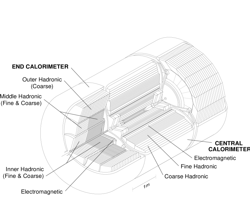
Figure 1: General view of DØ  calorimeters.

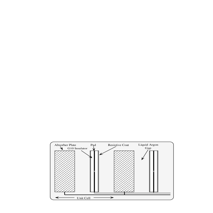
Figure 2: Diagram of a DØ calorimeter unit cell.

A general view of the DØ calorimeters is displayed in Fig. 1, showing the different electromagnetic and hadronic sections. The cells are constructed of uranium absorber plates interleaved with Cu/G10 readout boards. The gaps are filled with LAr as the active medium. A cross section of a unit cell is shown in Fig. 2. The coarse hadronic sections are made of copper or steel instead of uranium. A side view of the DØ calorimeters is shown in Fig. 3. DØ defines a coordinate system with the origin at the geometric center of the detector and the $z$ axis along the direction of the proton beam. The transverse plane is defined by the cartesian axes $x$ and $y$. In spherical coordinates, the three coordinates are described by the radius $r$, the azimuthal angle $\varphi$, and the polar angle $\theta$. Pseudorapidity is defined as $\eta=-\ln[{\mathrm{t}an}(\theta/2)]$. The segmentation in $\Delta\eta\times\Delta\varphi$ space is 0.1$\times$0.1, or 0.05$\times$0.05 at shower maximum (third electromagnetic layer).

The single particle energy resolutions for electrons ($e$) and charged pions ($\pi$) were measured from test beam data, and parameterized with a $(\sigma_{E}/E)^{2}=S^{2}/E+C^{2}$ functional form. For electrons, the sampling term $S$ is 14.8 (15.7)% in the CC (EC), and the constant term $C$ is 0.3% in both the CC and EC. For pions, the sampling term is 47.0 (44.6)%, and the constant term is 4.5 (3.9)% in the CC (EC) [6].

The energy of a jet measured in the calorimeters is distorted by uninstrumented regions, phenomena which affect the response, energy deposits in the liquid argon due to uranium decays, spectator interactions, reconstruction and resolution effects. The calorimeter response to the different types of particles is the most important aspect of the jet energy scale correction. Electromagnetically interacting particles, like photons ($\gamma$) and electrons, deposit most of their energy in the electromagnetic (EM) section of the calorimeters ($\sim 20.5$ radiation lengths thick). Hadrons, by contrast, lose energy primarily through nuclear interactions. The showers they cause are much longer than those from electromagnetic particles, and extend through the three sections of the calorimeter: EM, fine hadronic (FH), and coarse hadronic (CH). In general, the calorimeter response to the EM ($e$) and non-EM ($h$) components of hadron showers is not the same because there are different physics processes involved. Non-compensating calorimeters have a response ratio $e/h>1$, and suffer from non-Gaussian event-to-event fluctuations in the fraction of the energy lost through $\pi^{0}$ production ($f_{\mathrm{em}}$). In addition, $\langle f_{\mathrm{em}}\rangle$ increases logarithmically with energy. As a result, such calorimeters give a non-Gaussian signal distribution for monoenergetic hadrons. Moreover, the signal is not linearly proportional to the hadron energy (non-linearity), and $e/\pi$ (ratio of electron to pion response) is energy dependent [7].

The DØ calorimeters are nearly compensating, with an $e/\pi$ ratio less than 1.05 above 30 GeV. Figure 4 shows the $e/\pi$ ratio from a Monte Carlo [8, 9] simulation (open squares) and from test beam data (full circles). The calorimeters are also linear with energy, except at very low energy, as illustrated in Fig. 5 from test beam data. Figure 6 shows the Gaussian behavior of the variable $(E_{T1}-E_{T2})/(E_{T1}+E_{T2})$ for dijet events with average jet transverse energy $E_{T}$ of 140 GeV observed in the DØ calorimeters, where $E_{T1}$ and $E_{T2}$ are randomly ordered from the pair of leading transverse energy jets. This Gaussian signature is characteristic of the hermeticity and linearity of the DØ calorimeters.

3 Jet Measurement

Jets emerging from a hard interaction deposit energy in numerous cells in the calorimeter. To determine the jet energy, an algorithm is needed which assigns calorimeter cells to jets. The final measured jet energy depends on this algorithm or jet definition. In this paper, only a fixed cone algorithm is considered [10], with jet centroid and cone size defined as ($\eta_{\mathrm{jet}}$,$\varphi_{\mathrm{jet}}$) and ${\mathcal{R}}=\sqrt{(\varphi-\varphi_{\mathrm{j}et})^{2}+(\eta-\eta_{\mathrm{j}et})^{2}}$, respectively.

The process of reconstructing jets in the calorimeter is iterative. First, towers ($\Delta\eta\times\Delta\varphi=0.1\times 0.1$) containing $E_{T}$ of 1 GeV or more are used as seeds for finding preclusters, which are formed by adding neighboring towers within a radius of ${\mathcal{R}}=0.3$ to seed towers. The $\eta_{i}$ of each tower is calculated with respect to the interaction vertex, which is determined from the tracking system [5]. Next, a fixed cone of radius ${\mathcal{R}}$ is drawn around each precluster centered at its centroid. A new center is then calculated using the Snowmass Accord [11] definitions for both the jet angles and transverse energy:

$$\hskip 99.58464ptE_{T\mathrm{jet}} = \sum_{i}E_{T_{i}}\,,$$ (1)

$$\hskip 99.58464pt\varphi_{\mathrm{jet}} = \sum_{i}E_{T_{i}}\varphi_{i}/E_{T\mathrm{jet}}\,,$$ (2)

$$\hskip 99.58464pt\eta_{\mathrm{jet}} = \sum_{i}E_{T_{i}}\eta_{i}/E_{T\mathrm{jet}}\,.$$ (3)

The sums are over all towers contained in the cone. This process is repeated iteratively, always using the Snowmass Accord definition, replacing the previous seed or jet direction by the current one until the center becomes stable. In the final step, $\eta_{\mathrm{jet}}$ and $\varphi_{\mathrm{jet}}$ are recalculated using the following definition:

$$\hskip 56.9055pt\varphi_{\mathrm{jet}} = \tan^{-1}\left(\sum_{i}E_{y_{i}}/\sum_{i}E_{x_{i}}\right)$$ (4)

$$\hskip 56.9055pt\theta_{\mathrm{jet}} = \tan^{-1}\left(\sqrt{\sum_{i}E_{x_{i}}^{2}+\sum_{i}E_{y_{i}}^{2}}/\sum_{i}E_{z_{i}}\right)$$ (5)

where $E_{x_{i}}=E_{i}\sin\theta_{i}\cos\varphi_{i}$, $E_{y_{i}}=E_{i}\sin\theta_{i}\sin\varphi_{i}$, and $E_{z_{i}}=E_{i}\cos\theta_{i}$. The transverse energy of a jet is still the sum of the transverse energies in each calorimeter tower inside the cone. Those jets with $E_{T}<8\;{\mathrm{G}eV}$ are discarded. Overlapping jets are merged into a single jet if more than 50$\%$ of the $E_{T}$ of the lower energy jet is contained in the overlap region. Otherwise, the energy of each cell in the overlap region is assigned to the nearest jet.

The particle level jet energy is defined as the energy of a jet found from final state particles using a similar cone algorithm to that used at the calorimeter level. The particle jet is never observed in data because it gets distorted when it interacts with the calorimeter material. But it can be clearly defined in a Monte Carlo sample by clustering together the final state particles, instead of calorimeter cells, into a fixed cone size. The particle jet includes only particles arising from partons participating in the hard scatter. The purpose of the jet energy scale calibration is to correct observed jets to the particle level.

3.1 Jet Energy Scale

The conversion from electronic ADC counts to energy and the layer-to-layer calibration are performed at the data reconstruction level and are based on test beam data. Detailed information on calorimeter performance and calibration can be found in Ref. [6].

This paper describes an in situ calibration based primarily on reconstructed collider data. This calibration relates the observed jet energy to that of the final state particle jet on average. The linearity and hermeticity of the DØ calorimeters provide Gaussian response functions and, therefore, allow separation of the jet energy resolution from the jet energy scale correction. Thus, the following sections focus on the scale correction and leave aside resolution effects. The DØ jet energy calibration is based almost entirely on data measurements, exploiting conservation of transverse momentum through an accurate determination of the event ${\hbox{$E$\kern-6.00006pt\lower-0.43057pt\hbox{/}}}_{T}$.

The particle level or true jet energy $E_{\mathrm{jet}}^{\mathrm{ptcl}}$ is obtained from the measured jet energy $E_{\mathrm{jet}}^{\mathrm{meas}}$ using the following relation:

$$E_{\mathrm{jet}}^{\mathrm{ptcl}}=\frac{E_{\mathrm{jet}}^{\mathrm{meas}}-E_{\mathrm{O}}({\mathcal{R}},\eta,{\mathcal{L}})}{R_{\mathrm{jet}}({\mathcal{R}},\eta,E)S({\mathcal{R}},\eta,E)}\,,$$ (6)

where:

• $E_{\mathrm{O}}({\mathcal{R}},\eta,{\mathcal{L}})$ is an offset, which includes the physics underlying event, noise from the radioactive decay of the uranium absorber, the effect of previous crossings (pile-up), and the contribution of additional $p\overline{p}$ interactions. The physics underlying event is defined as the energy contributed by spectators to the hard parton interaction which resulted in the high-$p_{T}$ event. The offset increases as a function of the algorithm cone size ${\mathcal{R}}$. The dependence on luminosity, ${\mathcal{L}}$, arises from the contribution of additional interactions. $E_{\mathrm{O}}$ is also parameterized as a function of $\eta$, measured with respect to the vertex of the interaction (physics $\eta$).

• $R_{\mathrm{jet}}({\mathcal{R}},\eta,E)$ is the energy response of the calorimeter to jets. It is parameterized as a function of jet energy after the offset subtraction. $R_{\mathrm{jet}}$ is independent of the algorithm cone size; however, its parameterization versus jet energy is cone size dependent because larger cones encompass a larger fraction of the energy of the cluster. Because the various detector components are not identical, $R_{\mathrm{jet}}$ is also dependent on detector pseudorapidity, that is $\eta$ calculated from the geometric center of the detector and not the interaction vertex. $R_{\mathrm{jet}}$ is typically less than one, due to energy lost in uninstrumented regions between modules, differences between electromagnetic and nuclear interacting particles ($e/h>1$), and module-to-module inhomogeneities.

• $S({\mathcal{R}},\eta,E)$ is the fraction of the particle jet energy that is deposited inside the algorithm cone. The jet energy is corrected back to the particle level, and therefore calorimeter showering effects must be removed. $S$ is less than one, meaning that the effect of showering is a net flux of energy from the inside to outside the cone. $S$ depends strongly on the cone size ${\mathcal{R}}$, energy, and $\eta$. It is parameterized as a function of jet energy after offset subtraction and response correction, and binned in terms of physics $\eta$.

  Most of the examples presented in this paper correspond to jets reconstructed with a ${\mathcal{R}}=0.7$ fixed cone algorithm. Jets reconstructed with other cone sizes or at $\sqrt{s}=630\;{\mathrm{G}eV}$ were also calibrated. This information is included in Refs. [3, 4].

4 Offset Correction

The $p\overline{p}$ inelastic collisions are classified as non-diffractive, single diffractive and double diffractive. An inelastic non-diffractive collision, also sometimes called hard core interaction, is an event in which both the proton and the anti-proton break up. A particular case of a hard core interaction is high-$p_{T}$ or hard parton scattering.

The offset correction is determined for non-diffractive events. It subtracts energy which is not associated with the high-$p_{T}$ interaction. This excess energy includes the contributions of uranium noise, pile-up, and additional $p\overline{p}$ interactions. Pile-up is the residual energy from previous $p\overline{p}$ crossings, which results from the long shaping times of electronic signals in calorimeter readout cells. Pile-up depends on the number of interactions in the previous beam crossings, and is therefore luminosity dependent. The underlying event includes soft interactions between spectator partons that constituted the colliding proton and anti-proton. This energy can be subtracted or not, depending on the characteristics of each particular physics measurement.

A crossing selected by a high-$p_{T}$ trigger can be modeled as the sum of a hard parton scattering overlaid with a zero bias (ZB) event at the same luminosity. The ZB trigger accepts every $p\overline{p}$ crossing, regardless of whether or not it contains an actual collision. The average number of hard interactions in a high-$p_{T}$ event, $\langle N\rangle$, may be written as:

$$\langle N\rangle=1+\langle N_{\mathrm{ZB}}\rangle\,.$$ (7)

Here, $\langle N_{\mathrm{ZB}}\rangle$ is the average number of hard core interactions in a ZB event and can be expressed as:

$$\langle N_{\mathrm{ZB}}\rangle=\sum_{n=0}^{\infty}n\,P(n)\,,$$ (8)

where the probability of having $n$ hard core collisions at a given luminosity, $P(n)$, follows a Poisson distribution.

The total offset correction, $E_{\mathrm{O}}$, can be presented as the sum:

$$\hskip 85.35826ptE_{\mathrm{O}} = (1+\langle N_{\mathrm{ZB}}\rangle)E_{\mathrm{ue}}+E_{\mathrm{noise}}+E_{\mathrm{pile}}$$ (9)

$$= E_{\mathrm{ue}}+\langle N_{\mathrm{ZB}}\rangle E_{\mathrm{ue}}+E_{\mathrm{noise}}+E_{\mathrm{pile}}\,,$$

where $E_{\mathrm{ue}}$ is the energy associated with the physics underlying event, $\langle N_{\mathrm{ZB}}\rangle E_{\mathrm{ue}}$ is the contribution to the underlying event from additional $p\overline{p}$ interactions, $E_{\mathrm{noise}}$ is the energy from uranium decay, and $E_{\mathrm{pile}}$ is the pile-up energy. For the actual correction, the last three terms may be combined, yielding:

$$E_{\mathrm{O}}=E_{\mathrm{ue}}+E_{\Theta}\,.$$ (10)

4.1 Physics Underlying Event

The energy from spectator partons is measured using low luminosity minimum bias (MB) data (${\mathcal{L}}=0.1\times 10^{30}\;{\mathrm{c}m}^{-2}{\mathrm{s}ec}^{-1}$). The MB trigger requires an inelastic collision in which both the proton and the anti-proton break up. MB events are, therefore, dominated by hard core interactions. The $E_{T}$ density per increment $\Delta\eta\times\Delta\varphi$ in MB events, $D_{\mathrm{MB}}$, is a measure of the transverse $E_{\mathrm{ue}}+E_{\mathrm{noise}}+E_{\mathrm{pile}}$ density. The contribution of uranium noise and pile-up, $D_{\mathrm{ZB}}^{{\mathrm{no\,HC}}}$, is measured in a low luminosity ZB sample with the requirement that there is no hard interaction. $D_{\mathrm{ue}}$ is then:

$$D_{\mathrm{ue}}=D_{\mathrm{MB}}-D_{\mathrm{ZB}}^{\mathrm{no\,HC}}\,.$$ (11)

It depends both on the center-of-mass energy and pseudorapidity. The energy to be subtracted from a jet, $E_{\mathrm{ue}}$, is $D_{\mathrm{ue}}\times A_{\eta,\varphi}$, where $A_{\eta,\varphi}$ is the area of the jet in $\eta$-$\varphi$ space. Figure 7 shows the dependence of $D_{\mathrm{ue}}$ on physics $\eta$ for both $\sqrt{s}=1800\;{\mathrm{G}eV}$ and $\sqrt{s}=630\;{\mathrm{G}eV}$ collisions. The uneven shape results from imperfect calibration of the intercryostat detector and loss of EM coverage in the intercryostat region. Because the physics underlying event is associated with the soft interactions in a single $p\overline{p}$ collision, it is independent of luminosity and of the number of $p\overline{p}$ interactions in the event.

4.2 Uranium Noise, Pile-up, and Extra Interactions

The contribution to the offset from uranium noise, pile-up, and additional $p\overline{p}$ interactions, $D_{\Theta}$, is the measured $E_{T}$ density in a ZB sample. Figure 8 displays parameterizations of $D_{\Theta}$ as a function of physics $\eta$ for different luminosities.

$D_{\Theta}$ also depends on the occupancy, defined as the number of calorimeter cells which were read out after zero-suppression divided by the total number of cells in the jet. Zero-suppression is the mechanism that suppresses cells with energy depositions inside a 2$\sigma$ window around the average pedestal value. Therefore, $D_{\Theta}$ from the ZB data must be extrapolated to a value consistent with average occupancies for jet data. This difference in occupancy dominates the uncertainty in the offset correction. It contributes an error of $\pm$ 0.25 GeV to $D_{\Theta}$. In addition, statistical and systematic errors in fitting the data are approximately 8%.

5 Response: The Missing $E_{T}$ Projection Fraction Method

The jet reconstruction algorithm maps charge collected in the liquid argon to energy. It is based on single particle test beam data, assuming ideal instrumentation and a linear response. The overall response after reconstruction is, however, less than unity, due to a non-linear response to low energy particles, dead material, and module-to-module response fluctuations. This section describes the missing $E_{T}$ projection fraction method [13] developed to measure the calorimeter response to jets in reconstructed data.

5.1 Definitions

DØ makes a direct measurement of the jet energy response, using conservation of $p_{T}$ in photon-jet ($\gamma$-jet) events. These events are composed of one photon balanced in $p_{T}$ by one or more jets. The missing transverse energy, ${\hbox{$\pol{E}$\kern-6.00006pt\lower-0.43057pt\hbox{/}}}_{T}$, is defined as:

$$\mbox{${\hbox{$\pol{E}$\kern-6.00006pt\lower-0.43057pt\hbox{/}}}_{T}$}=-\left(\sum_{i}E_{x_{i}},\sum_{i}E_{y_{i}}\right)\,,$$ (12)

where $E_{x_{i}}$, $E_{y_{i}}$ are defined as in Section 3 and $i$ runs over all calorimeter cells with $|\eta|<4.5$. This definition implies that the energy deposit in each cell may be treated as though it were deposited by a zero mass particle, so that ${\hbox{$\pol{E}$\kern-6.00006pt\lower-0.43057pt\hbox{/}}}_{T}$$=$${\hbox{$\pol{p}$\kern-3.99994pt\lower-0.43057pt\hbox{/}}}_{T}$. In an ideal calorimeter, any non-zero ${\hbox{$E$\kern-6.00006pt\lower-0.43057pt\hbox{/}}}_{T}$ indicates the presence of particles which failed to deposit their energy in the detector, such as neutrinos or high-$p_{T}$ muons. For a photon-jet event in a real detector, a non-zero ${\hbox{$E$\kern-6.00006pt\lower-0.43057pt\hbox{/}}}_{T}$ measures the overall imbalance of transverse energy in the calorimeter due to differences in response to photons and jets. This can be used to measure the calorimeter response to jets, $R_{\mathrm{jet}}$, relative to the precisely known photon response.

In $\gamma$-jet events, the particle level or true photon and recoil transverse energies $E_{T\gamma}$ and $E_{T\mathrm{recoil}}$, satisfy:

$$\pol{E}_{T\gamma}+\pol{E}_{T\mathrm{recoil}}=0\,.$$ (13)

In a real calorimeter, however, the photon and jet responses ($R_{\mathrm{e}m}$ and $R_{\mathrm{r}ecoil}$) are both less than unity, and the equation is modified to:

$$\pol{E}_{T\gamma}^{\mathrm{m}eas}+\pol{E}_{T{\mathrm{r}ecoil}}^{\mathrm{m}eas}=-\pol{\mbox{${\hbox{$E$\kern-6.00006pt\lower-0.43057pt\hbox{/}}}_{T}$}}^{\mathrm{m}eas}\,,$$ (14)

where $\pol{E}_{T\gamma}^{\mathrm{m}eas}=R_{\mathrm{e}m}\pol{E}_{T\gamma}$ and $\pol{E}_{T{\mathrm{r}ecoil}}^{\mathrm{m}eas}=R_{\mathrm{r}ecoil}\pol{E}_{T{\mathrm{r}ecoil}}$. The energy scale for electromagnetically interacting particles is determined [14] from the $Z\rightarrow e^{+}e^{-}$, $J/\psi$, and $\pi^{0}$ data samples, using the known masses of these resonances. If $\pol{E}_{T\gamma}^{\mathrm{m}eas}$ is corrected for energy scale in the $\gamma$-jet data sample, Eq. 14 transforms into:

$$\hskip 71.13188pt\pol{E}_{T\gamma}+R_{\mathrm{recoil}}\pol{E}_{T\mathrm{recoil}} = -\pol{\mbox{${\hbox{$E$\kern-6.00006pt\lower-0.43057pt\hbox{/}}}_{T}$}}\,$$

$$\hskip 71.13188pt\pol{E}_{T\gamma}+R_{\mathrm{recoil}}\hat{n}_{T\gamma}\cdot\pol{E}_{T\mathrm{recoil}} = -\hat{n}_{T\gamma}\cdot\mbox{${\hbox{$\pol{E}$\kern-6.00006pt\lower-0.43057pt\hbox{/}}}_{T}$}\,$$

$$\hskip 71.13188pt1+R_{\mathrm{recoil}}\frac{\hat{n}_{T\gamma}\cdot\pol{E}_{T\mathrm{recoil}}}{E_{T\gamma}} = -\frac{\hat{n}_{T\gamma}\cdot\mbox{${\hbox{$\pol{E}$\kern-6.00006pt\lower-0.43057pt\hbox{/}}}_{T}$}}{E_{T\gamma}}\,,$$ (15)

where $\hat{n}_{T\gamma}=\pol{E}_{T\gamma}/|\pol{E}_{T\gamma}|$, and ${\hbox{$\pol{E}$\kern-6.00006pt\lower-0.43057pt\hbox{/}}}_{T}$ is the missing transverse energy recalculated after the photon correction. Eq. 13 can be written as $\pol{E}_{T\gamma}=-\hat{n}_{T\gamma}\cdot\pol{E}_{T\mathrm{recoil}}$; then $R_{\mathrm{recoil}}$ is:

$$R_{\mathrm{recoil}}=1+\frac{\mbox{${\hbox{$\pol{E}$\kern-6.00006pt\lower-0.43057pt\hbox{/}}}_{T}$}\cdot\hat{n}_{T\gamma}}{E_{T\gamma}}\,.$$ (16)

In the special case of a $\gamma$-jet two body process, and in the absence of offset and showering effects, $R_{\mathrm{recoil}}$ would be the ratio $E_{T\mathrm{jet}}^{\mathrm{meas}}/E_{T\mathrm{jet}}^{\mathrm{ptcl}}$ of measured to particle jet transverse energies. In the presence of offset and showering losses, $R_{\mathrm{recoil}}$ is the energy response of the calorimeter to jets, $R_{\mathrm{j}et}$, where “jet” is the leading jet of the event. This is a good approximation if the difference in azimuth between the $\gamma$ and the leading jet is close to $\pi$.

5.2 The Energy Estimator, $E^{\prime}$

$R_{\mathrm{jet}}$ is measured at DØ as $R_{\mathrm{r}ecoil}$ from a $\gamma$-jet sample, using conservation of transverse momentum (the terms transverse momentum and transverse energy are used interchangeably). The response is, however, dependent on jet energy rather than its transverse component. This is because $e/\pi$ and the particle composition of jets are energy dependent.

Measuring $R_{\mathrm{jet}}$ directly as a function of $E_{\mathrm{jet}}^{\mathrm{meas}}$ is problematic. The finite jet and photon energy resolutions, steeply falling photon cross section, trigger and reconstruction thresholds, and event topology contribute biases which must be removed. Most of these biases and smearing effects are reduced to negligible levels by binning the response not in $E_{\mathrm{jet}}^{\mathrm{meas}}$ but instead in some better measured quantity which is strongly correlated with $E_{T\mathrm{jet}}^{\mathrm{ptcl}}$. For this quantity the jet energy estimator $E^{\prime}$ is chosen and defined as:

$$E^{\prime}=E_{T\gamma}\cdot\cosh(\eta)\,,$$ (17)

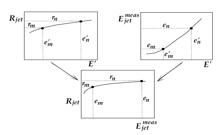
Figure 9: Derivation of $R_{\mathrm{jet}}$ versus $E_{\mathrm{jet}}^{\mathrm{meas}}$ using the energy estimator $E^{\prime}$.

where $E_{T\gamma}$ includes the electromagnetic scale correction. Both $E_{T\gamma}$ and the jet pseudorapidity are measured with high resolution compared to $E_{\mathrm{jet}}^{\mathrm{meas}}$ . After binning the response in terms of $E^{\prime}$, the dependence of $R_{\mathrm{jet}}$ on $E_{\mathrm{jet}}^{\mathrm{meas}}$ is obtained by measuring the average $E_{\mathrm{jet}}^{\mathrm{meas}}$ in each $E^{\prime}$ bin. Figure 9 illustrates the $E^{\prime}\rightarrow E_{\mathrm{jet}}^{\mathrm{meas}}$ mapping procedure.

5.3 Tests of the Method

The method is tested using a parametric simulation. The simulation generates $\gamma$-jet events according to a cross section with a given $E_{T}$ dependence. The energies of the photon and the jet are smeared and scaled with energy resolutions and responses measured from data.

Figure 10 (top) shows a comparison between $R_{\mathrm{jet}}$ determined from the simulation directly as a function of $E_{\mathrm{jet}}^{\mathrm{meas}}$ (open circles), and the same quantity binned in terms of $E^{\prime}$ and then mapped onto $E_{\mathrm{jet}}^{\mathrm{meas}}$ (closed circles). While the closed circles are in very good agreement with the input response (solid line), the open circles exhibit the smearing effect arising from a finite jet energy resolution. Figure 10 (bottom) shows excellent agreement between the fits to $R_{\mathrm{jet}}$ versus $E^{\prime}$ and the input function given different reasonable assumptions for the $E_{T}$ dependence of the photon cross section, such as $E_{T}^{-5}$,$E_{T}^{-4}$, and $E_{T}^{-2}$.

6 Response: Photon Sample Selection

A large event sample is necessary to measure the jet response of each calorimeter with a reasonably small uncertainty over a large range of energies. Thus, $R_{\mathrm{jet}}$ is measured from a collider data sample obtained by applying a set of cuts which retain a large sample while limiting the systematic biases. For the purpose of calibration, the “$\gamma$-jet” sample is not restricted to direct photon events. It also includes events with one jet well contained in the EM calorimeter and little nearby hadronic energy.

6.1 General Cuts

From the events with photon candidates accepted during data collection, only those with one or more reconstructed EM clusters are used. Events with noisy cells which fake or distort jets are rejected. The Main Ring, the injector for the Tevatron, passes through the hadronic calorimeter and is active during data taking for $\overline{p}$ production. Events containing particles related to Main Ring activity are, therefore, removed from the sample. The muon system is used as a loose veto to avoid events with bremsstrahlung photons from cosmic ray muons. If the leading photon $E_{T}$ is less than 30 GeV, there must be no reconstructed muons in the event; otherwise the event is accepted if muons have $p_{T\mu}<100\;{\mathrm{G}eV/c}$. Because events with primary vertices far from the center of the detector can distort $E_{T}$ measurements, the $z$-coordinate of the vertex must satisfy $|z|<70\;{\mathrm{c}m}$.

Fiducial cuts on detector $\eta$ are applied to ensure good containment of the EM cluster inside the calorimeters ($|\eta|<1$ or $1.6<|\eta|<2.5$). Candidates near detector boundaries are also rejected. There must be at least one reconstructed jet in the event, and the leading jet must be contained in the CC ($|\eta|<0.7$) or the EC ($1.8<|\eta|<2.5$) for the CC and EC calibrations, respectively.

There are two types of background to the calibration sample, removed as described below.

6.1.1 Instrumental Background

The instrumental background is contributed by events in which the photon, or pair of photons from a highly EM jet (mostly $\pi^{0}$ jets), is not well isolated from a significant amount of hadronic energy. The following variables are used in the selection procedure to remove background:

• The fraction of the cluster $E_{T}$ deposited in the EM layers of the calorimeters, EMF.

• The cluster isolation in the plane transverse to the beam, $f_{\mathrm{i}so}$, defined as:

  $$f_{\mathrm{i}so}\equiv\frac{E_{\mathrm{t}ot}({\cal R}=0.4)-E_{\mathrm{e}m}({\cal R}=0.2)}{E_{\mathrm{e}m}({\cal R}=0.2)}\,,$$

  where $E_{\mathrm{t}ot}$ and $E_{\mathrm{e}m}$ are the total energy and the EM energy within a cone radius ${\cal R}$.

• The total charge in the transition radiation detector [5], $\varepsilon_{t}$, measured in units of the charge of the electron.

• The presence of a track in a road projected from the EM calorimeter cluster through the tracking chambers to the event vertex. Track match significance, $\sigma_{\mathrm{t}rk}$, is defined as:

  $$\sigma_{\mathrm{t}rk}=\sqrt{\left(\frac{\Delta\varphi}{\sigma_{\Delta\varphi}}\right)^{2}+\left(\frac{\Delta z}{\sigma_{\Delta z}}\right)^{2}}\,,$$

  where $\Delta\varphi$ and $\Delta z$ are the distances between the track and the cluster along the azimuthal and beam directions.

• The ionization in the central tracking detectors, dE/dx, in units of minimum ionizing particles.

Table 1 shows the cuts on photon candidates to reject background. The three cuts based on tracking information, $\varepsilon_{t}$, $\sigma_{\mathrm{t}rk}$, and dE/dx must be satisfied for events with $E_{T\gamma}>25\;{\mathrm{G}eV}$ only if $\mbox{${\hbox{$E$\kern-6.00006pt\lower-0.43057pt\hbox{/}}}_{T}$}/E_{T\gamma}>0.65$. Instead, only one of the three is required if $E_{T\gamma}<25\;{\mathrm{G}eV}$ or $\mbox{${\hbox{$E$\kern-6.00006pt\lower-0.43057pt\hbox{/}}}_{T}$}/E_{T\gamma}<0.65$.

There is a bias in $R_{\mathrm{jet}}$ due to the presence of highly electromagnetic jets in the sample, as compared to photons. This bias is studied using a $\chi^{2}$ test [12], which measures the consistency of the shower shape of the calibration sample with that expected from an electromagnetic shower. A matrix is constructed with transverse and longitudinal shower shape information from the photon candidate, and then compared with the same type of matrix built from electromagnetic clusters in a Monte Carlo sample. A cut on $\chi^{2}$ removes a significant number of events but is a good discriminator between real photons and highly electromagnetic jets. Figure 11 shows the magnitude of the instrumental background bias on the jet response. As the cut on $\chi^{2}$ tightens, the fraction of real photons in the sample increases, but the response changes only slightly. So that a large sample can be retained, a $\chi^{2}$ cut is not applied in the event selection procedure, and a bias on the order of 0.7% towards a larger response is present. A large fraction of this bias cancels against the topology bias, as will be discussed in Section 8.

6.1.2 Physics Backgrounds

The physics backgrounds include Drell-Yan, $Z\rightarrow e^{+}e^{-}$, and $W\rightarrow e\nu$ events. In events with two electromagnetic clusters, such as $Z$ $\rightarrow$ $e^{+}e^{-}$ production, $R_{\mathrm{jet}}$ is approximately unity. The effect of the $Z$ boson background can be determined by applying a cut on the dielectron invariant mass, $m_{ee}$. This background is very small and, therefore, the cut $75\;{\mathrm{G}eV/c}^{2}<m_{ee}<105\;{\mathrm{G}eV/c}^{2}$ produces a negligible change in the measured response.

$W\rightarrow e\nu$ events have a large ${\hbox{$\pol{E}$\kern-6.00006pt\lower-0.43057pt\hbox{/}}}_{T}$ in the direction of the neutrino, so they are not useful for calibration purposes. They are removed using the tracking cuts listed in Table 1, combined with a ${\hbox{$E$\kern-6.00006pt\lower-0.43057pt\hbox{/}}}_{T}$ cut, as described before. After the cuts, the remaining bias on $R_{\mathrm{jet}}$ due to physics background, determined from Monte Carlo and data samples, is $\mathrel{\hbox to0.0pt{\lower 4.0pt\hbox{\hskip 1.0pt$\sim$}\hss}\raise 1.0pt\hbox{$<$}}$ 0.5%.

6.2 Topology Cuts

The relation $R_{\mathrm{jet}}=R_{\mathrm{recoil}}$, where the subscript jet refers to the leading jet in the $\gamma$-jet event, is exact only in the case of a two body process. Photon events may contain more than one reconstructed jet along with a number of energy clusters which are not reconstructed as jets. Variations in topology, therefore, contribute a systematic error to the response measurement.

To remove this topology bias, the photon and the leading jet must have a difference greater than 2.8 radians in azimuth. The residual error is investigated by studying the change in response for different energy bins as the $\Delta\varphi$ cut is varied from $2.1$ to $3.1$ radians. Figure 12 shows the change in $R_{\mathrm{jet}}$ as the $\Delta\varphi$ cut is tightened for the $50<E^{\prime}<60\;{\mathrm{G}eV}$ bin. The circles correspond to an integrated distribution (lower $\Delta\varphi$ bins include the events of the higher $\Delta\varphi$ bins), while the open squares represent the differential distribution. Requiring $\Delta\varphi>2.8$ radians is a good compromise between a large event sample and bias minimization. The residual error after the cut is estimated with the parameterizations to the integrated (linear fit) and differential distributions (exponential fit). The fractional difference between $R_{\mathrm{jet}}$ at $\Delta\varphi=\pi$ and $\Delta\varphi>2.8$ radians is an estimate of the remaining topology bias. This difference as a function of $E^{\prime}$ is plotted in Fig. 13 for both the CC and the EC. The plots show that, after requiring $\Delta\varphi>2.8$ radians, the remaining bias is approximately 0.5-1% towards a lower response and consistent with a constant dependence on $E^{\prime}$. A large fraction of this bias cancels against the effect of instrumental background, as will be discussed in Section 8.

6.3 Multiple Interaction Cuts

Events which consist of several overlaid interactions are called multiple interaction events. Usually, only the “primary” interaction will produce high-$E_{T}$ objects. The additional interactions can, however, degrade the accuracy of the vertex determination for the primary interaction. On average, jets reconstructed with an incorrect vertex are assigned a higher pseudorapidity, yielding a larger event $E^{\prime}$ and a lower jet $E_{T}$. The overall effect is an increase of the ${\hbox{$E$\kern-6.00006pt\lower-0.43057pt\hbox{/}}}_{T}$ in the direction of the jet, thus lowering the measured response. This effect grows as luminosity increases, as a result of the increasing proportion of multiple interaction crossings.

To reduce this bias, a low luminosity sample is used. This sample, however, still contains a number of multiple interaction events. These are removed by requiring the trigger, tracking detectors, and calorimeter information to be consistent with a single interaction. Figure 14 shows the change in the measured response from a low luminosity sample when the single interaction requirement is applied. The low tails in the $R_{\mathrm{jet}}$ distributions are removed by this cut.

To measure any residual luminosity dependence of the response after the single interaction cut, the response is measured as a function of luminosity for various $E^{\prime}$ bins for CC and EC jets, as shown in Figs. 15 and 16. A linear fit of $R_{\mathrm{jet}}$ versus ${\mathcal{L}}$ allows an extrapolation to zero luminosity. In Fig. 15, the CC data show very little sensitivity to luminosity. The EC data, however, show a slight trend to lower response with increasing luminosity. The estimated difference in response between a luminosity of $5\times 10^{30}\;{\mathrm{c}m}^{-2}{\mathrm{s}ec}^{-1}$ and zero is approximately 0.5% for the EC jets. Because the sample used in this analysis is integrated over this range of luminosities, any residual luminosity effects are less than 0.25%.

7 Response: Rapidity Dependence

After test beam calibration, the DØ calorimeter system still shows non-uniform regions in pseudorapidity. Given that most physics measurements need a high level of accuracy at all rapidities, $\eta$-dependent corrections become necessary. These are the cryostat factor and the IC corrections applied in consecutive order to both the jet energy and the event ${\hbox{$\pol{E}$\kern-6.00006pt\lower-0.43057pt\hbox{/}}}_{T}$.

The $\eta$-dependent corrections are applied as multiplicative factors to the jet energy. Given that the energy corrections are not derived for calorimeter cells but for physics objects, it is not possible to recalculate ${\hbox{$\pol{E}$\kern-6.00006pt\lower-0.43057pt\hbox{/}}}_{T}$ using the definition in Section 5. Instead, the corrected missing transverse energy, $\mbox{${\hbox{$\pol{E}$\kern-6.00006pt\lower-0.43057pt\hbox{/}}}_{T}$}^{\mathrm{c}orr}$, is determined by adding to the measured or reconstructed missing transverse energy, $\mbox{${\hbox{$\pol{E}$\kern-6.00006pt\lower-0.43057pt\hbox{/}}}_{T}$}^{\mathrm{m}eas}$, the difference between the uncorrected and the corrected vector sums of the $E_{T}$ of the individual physics objects (jets and photons in the calibration sample). In other words:

$$\mbox{${\hbox{$\pol{E}$\kern-6.00006pt\lower-0.43057pt\hbox{/}}}_{T}$}^{\mathrm{corr}}=\mbox{${\hbox{$\pol{E}$\kern-6.00006pt\lower-0.43057pt\hbox{/}}}_{T}$}^{\mathrm{meas}}+\sum_{\gamma}\left(\pol{E}_{T\gamma}^{\mathrm{meas}}-\pol{E}_{T\gamma}^{\mathrm{corr}}\right)+\sum_{\mathrm{jet}}\left(\pol{E}_{T\mathrm{jet}}^{\mathrm{meas}}-\pol{E}_{T\mathrm{jet}}^{\mathrm{corr}}\right)\,.$$ (18)

This formula depends on the jet algorithm because it is based on reconstructed physics objects instead of calorimeter cells. It is, however, a good approximation to the ${\hbox{$E$\kern-6.00006pt\lower-0.43057pt\hbox{/}}}_{T}$ corrected for the photon scale and the rapidity dependence of jet response, if the jet cone size is large (${\mathcal{R}}$=0.7).

7.1 Cryostat Factor Correction

The cryostat factor, $F_{\mathrm{cry}}$, is defined as the ratio $R_{\mathrm{jet}}^{\mathrm{EC}}/R_{\mathrm{jet}}^{\mathrm{CC}}$. $F_{\mathrm{cry}}$ is expected to be independent of $E^{\prime}$ because the construction of the CC and the EC is similar. The measured response versus $E^{\prime}$ before corrections is shown in Fig. 17. $R_{\mathrm{jet}}$ is plotted in three detector $\eta$ regions: CC ($|\eta|<0.7$), IC ($0.7<|\eta|<1.8$), and EC ($1.8<|\eta|<2.5$).

$F_{\mathrm{cry}}$ is measured where the CC and the EC data overlap, in the range $60\;{\mathrm{G}eV}<E^{\prime}<180\;{\mathrm{G}eV}$. In the EC data, an additional cut $E_{T\gamma}>25\;{\mathrm{G}eV}$ is necessary to remove the reconstruction threshold bias due to jet finite energy resolution. $F_{\mathrm{cry}}$ is measured separately in the EC north ($-2.5<\eta<-1.8$) and the EC south ($1.8<\eta<2.5$) calorimeters. The ratio $F_{\mathrm{cry}}^{\mathrm{N}}/F_{\mathrm{cry}}^{\mathrm{S}}=0.997\pm 0.003$ shows that $F_{\mathrm{cry}}$ is the same in both EC’s within errors. Figure 18 shows the measured value for the cryostat factor, $F_{\mathrm{cry}}=0.980\pm 0.007$ (stat), and illustrates its derivation from a fit of a constant function to the measured $R^{\mathrm{EC}}_{\mathrm{jet}}/R^{\mathrm{CC}}_{\mathrm{jet}}$ versus $E^{\prime}$.

The most important consequence of the independence of $F_{\mathrm{cry}}$ on $E^{\prime}$ is the possibility of using EC data to extend the range of the CC response measurement. This is possible because forward jets have higher energies than central jets with the same $E_{T}$. Thus, the energy range of the response measurement can be extended from $\sim 150\;{\mathrm{G}eV}$ to nearly 300 GeV.

7.2 IC Correction

The intercryostat region, covering the pseudorapidity range $0.8<|\eta|<1.6$, is the least well instrumented region of the calorimeter system. The IC is a non-uniform region covered by different types of detectors. A substantial amount of energy is lost in the cryostat walls, module endplates, and support structures. Additionally, in the range $1.2<|\eta|<1.4$, the system lacks electromagnetic calorimetry and the total depth falls slightly below 6 interaction lengths. As a consequence, the response has a residual $\eta$ dependence in this region, even after the cryostat factor has been applied to EC jets.

7.2.1 Event Selection and Method

The IC correction to the response is measured using both $\gamma$-jet and jet-jet events. Because the dependence of the response on pseudorapidity is related to detector inhomogeneities, $R_{\mathrm{jet}}$ is measured as a function of detector pseudorapidity. For the $\gamma$-jet sample, the photon is kept central ($|\eta|<0.5$), while the jet $\eta$ is unconstrained. For the jet-jet sample, one of the two leading $E_{T}$ jets is required to be central ($|\eta|<0.5$), and there is no restriction on the $\eta$ of the other jet. In this case, $R_{\mathrm{jet}}$ is defined as:

$$R_{\mathrm{jet}}\equiv 1+\frac{\mbox{${\hbox{$\pol{E}$\kern-6.00006pt\lower-0.43057pt\hbox{/}}}_{T}$}\cdot\hat{n}_{\mathrm{central\,jet}}}{E_{T\,\mathrm{central\,jet}}}\,,$$ (19)

and is measured as a function of the jet detector $\eta$. The $\gamma$-jet events are used only at low jet $E_{T}$, as the sample is statistically limited at high $E_{T}$. The correction for high $E_{T}$ jets is determined from the jet-jet data. For two identical $E_{T}$ jets, one central and one far forward, it is more likely for the central $\eta$ jet to fluctuate to a higher measured $E_{T}$ than the forward jet. This is because, for the same $E_{T}$, forward jets have higher energies and, therefore better resolutions than central jets. In addition, forward jets are kinematically suppressed. This causes a bias in the jet-jet sample above $|\eta|=2$ which is removed with a cut on the product of the transverse energies of the two leading jets.

The IC correction is performed before the energy dependent response correction. Because the energy dependence of $R_{\mathrm{jet}}$ is folded into $R_{\mathrm{jet}}$ versus $\eta$, this function is not a constant even for a uniform detector (ideal $\eta$ dependence); it must be, however, smooth. After the cryostat factor correction is applied, the IC correction is determined by means of a smooth interpolation through the IC of a fit to the measured $R_{\mathrm{jet}}$ versus $\eta$ in the CC and the EC.

7.2.2 Results

To determine the ideal $\eta$ dependence of the response in the IC, the response is fit to the function $R_{\mathrm{jet}}=a+b\cdot\ln[\cosh(\eta)]$ in the CC and EC regions. This functional form is derived from the energy dependence of the response, which is well described by:

$$R_{\mathrm{jet}}=\alpha+b\cdot\ln E\,.$$ (20)

Thus:

$$\hskip 99.58464ptR_{\mathrm{jet}} = \alpha+b\cdot\ln(E_{T}\cdot\cosh\eta)$$ (21)

$$= \alpha+b\cdot\ln E_{T}+b\cdot\ln(\cosh\eta)\,.$$

Reordering terms, and for a fixed $E_{T}$ bin:

$$R_{\mathrm{jet}}=a+b\cdot\ln(\cosh\eta)\,.$$ (22)

The data are fit in the range $|\eta|<0.5$ and $2<|\eta|<2.5$. A cut on $E_{T1}\cdot E_{T2}$, which requires this product to be greater than the $E_{T}$ threshold for which a particular jet trigger is fully efficient, is applied to avoid the resolution bias in jet-jet data above $\eta=2$. The two halves of the detector, $\eta>0$ and $\eta<0$, are treated separately. Figures 19 and 20 show the measured $\eta$ dependence for jet-jet and $\gamma$-jet data respectively, along with the fit to an ideally uniform detector.

The correction is determined in bins of 0.1 in detector $\eta$. The difference between the fit to the ideal response and the measured value is used to obtain a correction factor $F_{\eta}$. Figure 21 shows $F_{\eta}$ as a function of the average central jet $E_{T}$ (${\mathcal{R}}=0.7$) for several $\eta$ bins. Also shown is a linear fit to the data, which is used to determine the correction factor as a function of jet $E_{T}$.

7.2.3 Error Analysis and Verification Studies

The accuracy of the IC correction is measured using the fact that the response versus $\eta$ should be constant after all corrections are applied. This is shown in Fig. 22, where the corrections applied to $R_{\mathrm{jet}}$ in $\gamma$-jet data are the offset, the cryostat factor, the IC, and the energy dependence (see Section 8). The horizontal line indicates the ideal $\eta$ dependence of the corrected $R_{\mathrm{jet}}$. Figure 22 also shows that the measured $R_{\mathrm{jet}}$ is slightly less than unity. The reason is that the correction to the ${\hbox{$E$\kern-6.00006pt\lower-0.43057pt\hbox{/}}}_{T}$ is only applied on found objects. As the unclustered energy is not corrected for response effects, the average total corrected transverse energy of the event is not expected to be exactly zero.

Figure 23 shows the response versus $\eta$ measured from jet-jet data after all corrections have been applied. The error on $F_{\eta}$ is determined from the residuals of the corrected $\gamma$-jet and jet-jet data with respect to the ideal $\eta$ dependence. Table 2 shows the means and RMS values for the residual distributions in $\gamma$-jet data, and Table 3 displays the means and RMS values for the residual distributions derived from jet-jet data. The values measured from each sample are in good agreement.

There is some evidence of a residual $\eta$ dependence beyond $|\eta|=2.5$ in the $\gamma$-jet measurements. This bias towards a lower response at high $|\eta|$ may be due to the breakdown of the constant cryostat factor approximation at very high pseudorapidity, or to energy lost down the beam pipe. To account for this effect, an additional $\eta$-dependent error is assigned. It starts from zero at $|\eta|=2.5$ and increases linearly up to $3\%$ at $|\eta|=3$.

The IC correction increases for decreasing cone sizes. It is determined separately for each cone size. Once the $\eta$-dependent corrections are applied to both the jet energy and the event ${\hbox{$\pol{E}$\kern-6.00006pt\lower-0.43057pt\hbox{/}}}_{T}$, the response becomes constant as a function of pseudorapidity to within $\sim$ 1% ($|\eta|<2.5$).

8 Response: Energy Dependence

In Section 2, the ratio $e/\pi$ was shown to be greater than unity and energy dependent. $R_{\mathrm{jet}}$ must, therefore, also be energy dependent. The energy dependence of $R_{\mathrm{jet}}$ at low to moderate $E^{\prime}$ ($E^{\prime}\mathrel{\hbox to0.0pt{\lower 4.0pt\hbox{\hskip 1.0pt$\sim$}\hss}\raise 1.0pt\hbox{$<$}}100\;{\mathrm{G}eV}$) is determined from low-$E_{T}$ photons and CC jets ($|\eta|<0.7$). For high $E^{\prime}$ ($\mathrel{\hbox to0.0pt{\lower 4.0pt\hbox{\hskip 1.0pt$\sim$}\hss}\raise 1.0pt\hbox{$>$}}100\;{\mathrm{G}eV}$), $R_{\mathrm{jet}}$ is measured from EC ($1.8<|\eta|<2.5$) jets, after $F_{\mathrm{cry}}$ and $F_{\eta}$ corrections are applied, taking advantage of the fact that the CC and EC are similarly constructed. In other words, the EC measurement is normalized to the CC measurement using $F_{\mathrm{cry}}$, in order to extend the energy reach of the global $R_{\mathrm{jet}}$ measurement. This Section starts with a discussion of the low-$E_{T}$ bias arising from reconstruction and resolution effects, and follows with a detailed description of the measurement of $R_{\mathrm{jet}}$ versus energy.

8.1 The Low-$E_{T}$ Bias

The combination of reconstruction inefficiencies, a minimum jet $E_{T}$ cut, and the finite jet energy resolution produces a bias in the measured response. At the $E_{T}$ threshold for jet reconstruction $E_{T}^{\mathrm{min}}$ (set at 8 GeV for all jet cone algorithms at DØ), the jet fractional $E_{T}$ resolution is approximately 50%. Thus, the net migration of low-$E_{T}$ jets to higher values is very large. At the same time, jets which fluctuate below $E_{T}^{\mathrm{min}}$ are not reconstructed. This low-end truncation biases the average jet $E_{T}$ to higher values, biases the ${\hbox{$E$\kern-6.00006pt\lower-0.43057pt\hbox{/}}}_{T}$ to lower values, and therefore biases the response to higher values. The jet reconstruction efficiency is less than unity due to inefficiencies in the algorithm for turning seed towers into jets. Consequently, the low-$E_{T}$ bias is present above the minimum jet $E_{T}$ reconstruction threshold (up to 20 GeV), and is both cone size and $\eta$-dependent.

Because the jet energy response is determined from the event ${\hbox{$\pol{E}$\kern-6.00006pt\lower-0.43057pt\hbox{/}}}_{T}$, $E_{T\gamma}$, and $\hat{n}_{\gamma}$, it may be measured without requiring any reconstructed jet in the event. To determine the effect of the bias, the response is measured as a function of $E_{T\gamma}$ for those events both with and without at least one reconstructed jet. The low-$E_{T}$ bias is then the ratio:

$$R_{\mathrm{bias}}=\frac{R_{\mathrm{jet(}\geq\mathrm{1\,jet)}}}{R_{\mathrm{jet(no\,jet\,required)}}}\,.$$ (23)

An independent estimate of the low-$E_{T}$ bias is obtained from simulated $\gamma$-jet events, constructed as in Section 5. The jet response is then “measured” using the missing $E_{T}$ projection fraction method. The low-$E_{T}$ bias is determined from the ratio of the response from a sample where the $E_{T}^{\mathrm{min}}$ cut is modeled to the response from a sample with no such restriction. This bias depends on the jet energy resolution, $E_{T}^{\mathrm{min}}$, and the reconstruction efficiency, while the offset and the $E_{T}$ dependence of the photon cross section contribute very little. Figure 24 compares the simulated bias and the data measurement for 0.7 cone jets. The results agree within the errors of the simulation (dotted band). The $R_{\mathrm{bias}}$ correction is obtained from parameterizations of the data measurements for different cone sizes, and the uncertainty is determined from the simulation.

8.2 Response versus $E^{\prime}$

After application of the low-$E_{T}$ bias, offset, cryostat factor, and IC corrections, $R_{\mathrm{jet}}$ is recalculated as a function of $E^{\prime}$ (Fig. 25). The average response in each $E^{\prime}$ bin is determined by fitting the response distribution with either a single or double Gaussian parameterization. A single Gaussian is sufficient for $E^{\prime}$ bins with less than 100 entries. These fits provide a response measurement less affected by misvertexing than the arithmetic means of the distributions because they are less sensitive to an occasional outlying point far from the peak. In Fig. 25, the points are plotted at the average value of $E^{\prime}$ within each bin. While the $\eta$ dependence of $R_{\mathrm{jet}}$ is dramatically reduced, as shown in Fig. 25, the IC is slightly lower compared to the CC and EC regions. Although the CC, IC, and EC responses are the same within the error of the $\eta$-dependent correction, only the most accurate CC and EC data are used to derive the jet response.

After determining the response versus $E^{\prime}$, a mapping between $E^{\prime}$ and the average jet energy is obtained separately for each jet algorithm. The mapping for 0.7 cone jets is shown in Fig. 26. The observed difference in this mapping between EC and CC jets is consistent with showering effects, as will be shown in Section 9.

8.3 Constraining High Energy Response with Monte Carlo

The jet energy response can be determined from the data for jets with energy up to $\sim 300\;{\mathrm{G}eV}$, as shown in Fig. 26. However, energy calibration is required for the highest energy jets in the data, nearly 600 GeV. The inclusion of Monte Carlo information at high energy is necessary in order to constrain the jet response extrapolated from the available data.

A set of $\gamma$-jet events was generated using herwig [15], processed through the geant-showerlib [16] fast detector simulation, and reconstructed with the standard photon and jet algorithms. showerlib is a library that contains single particle calorimeter showers obtained using the geant full detector simulation. Because geant is a time consuming computer package, the showerlib approach is convenient. The jet response as measured from this sample is inconsistent with the response as measured from data, as shown in Fig. 27. This is because the Monte Carlo does not correctly model the $e/\pi$ ratio (see Fig. 4 in Section 2). Therefore, a different approach is followed to generate the Monte Carlo points at high $E_{T}$.

The method consists of returning to the particle level jets in the Monte Carlo. For a given particle jet, the sum of the energies of all final-state particles in the jet cone gives the total energy of the jet. The detector may then be simulated by convoluting the particle jet with single particle test beam data. Each individual particle is scaled by the appropriate response measured from the test beam, parameterized in terms of energy. The response functions used are shown in Figs. 28a-c. Electrons and photons are scaled by the electron response, and $\pi^{0}$ mesons are scaled as two photons, each with half of the energy of the pion. All other particles are scaled by the response of charged pions. Note that there are no test beam data below 2 GeV. Figures 28a-c show three different assumptions for the behavior of the response in that low energy range. For comparison, Fig. 28d shows the single particle responses given by the showerlib Monte Carlo.

As a test, illustrated in Fig. 29, the showerlib Monte Carlo response as determined using the ${\hbox{$E$\kern-6.00006pt\lower-0.43057pt\hbox{/}}}_{T}$ projection fraction method is compared with the response derived from the single particle convolution method, using the Monte Carlo response functions (Fig. 28d). The two responses agree to within 1%. The shapes of the response curves derived from the three different assumptions shown in Figs. 28a-c are then compared with the shape of the response derived from data. As shown in Fig. 30, the best agreement is found from the model in Fig. 28b (extrapolated electron response, fixed pion response).

The model-dependent error in the extrapolation depends upon the lower cutoff energy for normalizing to the data. The two extreme single particle response models are used: the extrapolated and the fixed responses (Figs 28a and 28c respectively). The Monte Carlo curves are normalized to the entire energy range where data exist, as shown in Fig. 31. The assumption is that these two extreme models bound the true response in the region where no data are available. The response is estimated as the mean value of the two extreme models at 500 GeV, and the error due to choice of model (inner error bar) as the difference divided by $\sqrt{12}$ ($\sim$ 0.7%). To this, an uncertainty of $\sim 0.6$% is added linearly, based on the closure test illustrated in Fig. 29. The small normalization and fit errors are also included in the full error bar shown.

8.4 Response Fits

The response versus energy for 0.7 cone jets is shown in Fig. 32. The data are fit with the functional form:

$$R_{\mathrm{jet}}(E)=a+b\cdot\ln E+c\cdot(\ln E)^{2}\,.$$ (24)

A logarithmic functional form is motivated by the fact that the EM content of a hadronic shower slowly increases with increasing shower energy [17]. In the development of such a shower some fraction $\langle f_{\mathrm{em}}\rangle$ of the energy is spent in the production of $\pi^{0}$ and $\eta$ mesons. A hadronic shower, therefore, has both an electromagnetic and a non-electromagnetic component. As defined in Section 2, $e$ and $h$ are the responses of the calorimeter to the EM and non-EM components of a hadronic shower. If $\pi$ is the response to charged pions, then:

$$\frac{e}{\pi}=\frac{1}{\frac{h}{e}\,-\langle f_{\mathrm{em}}\rangle(\frac{h}{e}-1)},\,$$ (25)

where, in general, $\langle f_{\mathrm{em}}\rangle$ is reasonably well described by $\sim\alpha\cdot\ln E\;{\mathrm{(}GeV)}$. In a completely compensating calorimeter $e/h$=1, and the ratio $e/\pi$ is unity for all energies. If $e/h\neq$ 1, the ratio $e/\pi$ tends to one at high energies but grows exponentially as energy decreases. If $e=1$, then $\pi$ would be $a+b\cdot\ln E$.

The logarithmic behavior of $R_{\mathrm{j}et}$ versus energy is suggested by the test beam measured $e/\pi$ ratio as a function of beam energy [6], and verified directly from the measurement of $R_{\mathrm{jet}}$ using collider data. The inclusion of the $(\ln E)^{2}$ term in Eq. 24 improves the agreement of the fit with the data in the quickly varying low energy region, while preventing the slope of the function from rising faster than the data at high energies.

The three sets of points shown in Fig. 32 correspond to CC jet data (open circles), EC jet data (filled circles), and Monte Carlo data (star). The three lowest energy points have large errors (nearly fully correlated point-to-point in energy), as a result of the low-$E_{T}$ bias correction. They are not used in the fit which includes points above 30 GeV. The $\chi^{2}$ of the fit is 10 for 15 degrees of freedom. Table 4 lists the fit parameters for the various cone algorithms. The calorimeter response is the same for all cone sizes as expected, although the parametrizations are slightly different because each algorithm associates a different energy to the same cluster.

8.4.1 Errors from Response Fits

The errors in the fit parameters, listed in Table 4, represent one standard deviation uncertainties, calculated from the $\chi^{2}=\chi^{2}_{\mathrm{min}}+1$ surface in the parameter space. However, the probability for all fit parameters to simultaneously take on values within the one standard deviation region ($\chi^{2}=\chi^{2}_{\mathrm{min}}+1$) is significantly less than 68% [18]. To account for this reduced probability, a surface is mapped out in parameter space containing a region with a 68% probability for parameter fluctuations in all the response fits. For three parameters this corresponds to the surface defined by $\chi^{2}=\chi^{2}_{\mathrm{min}}+3.5$ [18]. The points lying on this surface are then mapped back onto the response versus energy plane. At each energy, the error is determined by the parameter set giving the greatest deviation from the nominal response. The result for the 0.7 cone algorithm is shown in Fig. 32.

The band represents the error on the fit to the response, and is used in place of one derived from the errors in Table 4. At high energy, it is only weakly dependent on the region where the fit is performed. Alternate functional forms were also investigated, giving results consistent with those from Eq. 24.

8.4.2 Error Correlations in Response Fit

The error of the fit on the jet response measurement dominates the systematic uncertainty over large regions of jet energy and pseudorapidity. In this section, the point-to-point correlations in uncertainty due to the fit errors described in the previous section are derived.

The error bands in Fig. 32 show the 68%-probability response at each energy based on fluctuations of all fit parameters. However, the parameter set that produces a given variation at one energy need not produce the same variation at any other energy in either magnitude or sign. In general, no single set of fit parameters may exist to produce the 68%-probability curves. But it is reasonable to expect that errors for two points of similar energy should be largely correlated. The correlations in the fit error are calculated as follows:

• A grid of parameter sets ($N_{\mathrm{grid}}$) is generated to define the $\chi^{2}\leq\chi^{2}_{\mathrm{min}}+3.5$ volume. This volume contains all fit parameter set fluctuations corresponding to a 68% probability content. Each parameter set defines a response function contained within the bands shown in Fig. 32.

• The parameter sets are used, noting the variation in response at 11 values of uncorrected jet energy between 10 and 500 GeV. The correlations in response for each pair of energy values are calculated from the parameter sets in the grid, which are used to define a correlation matrix for the 11 energy values. Each element of the matrix ($\rho(i,j)$) is the standard correlation coefficient between the responses measured at each energy value, and defined as:

  $$\rho(i,j)=\frac{\sum_{n=1}^{N_{\mathrm{grid}}}(R_{n}(i)-\overline{R(i)})(R_{n}(j)-\overline{R(j)})}{[\sum_{n=1}^{N_{\mathrm{grid}}}(R_{n}(i)-\overline{R(i)})^{2}\sum_{n=1}^{N_{\mathrm{grid}}}(R_{n}(j)-\overline{R(j)})^{2}]^{\frac{1}{2}}}\,,$$ (26)

  where $R(i)$ is the response for the $i^{\mathrm{th}}$ energy bin.

Table 5 shows the correlation matrix for the response fit to 0.7 cone jets. Correlations are illustrated graphically in Fig. 33, where four rows of the matrix are plotted, showing the error correlations relative to the errors at 20, 50, 100, and 500 GeV respectively.

8.5 Shower Containment

The DØ central and end calorimeters are more than 7.2 and 8 interaction lengths ($\lambda_{\mathrm{INT}}$) thick, respectively. Although the EC is thick enough to contain all expected showers, there may be some leakage out of the CC for very high energy jets. Because the energy not contained within the calorimeter contributes to ${\hbox{$E$\kern-6.00006pt\lower-0.43057pt\hbox{/}}}_{T}$, the measured response in principle corrects for leakage. The response of jets with energy less than $\sim 100\;{\mathrm{G}eV}$ is measured using the CC and, therefore, includes the containment correction. For jets with energy $\mathrel{\hbox to0.0pt{\lower 4.0pt\hbox{\hskip 1.0pt$\sim$}\hss}\raise 1.0pt\hbox{$>$}}100\;{\mathrm{G}eV}$, the response is determined from EC data. Measuring the high energy response in the end cap calorimeter, with full containment, and applying it to the central calorimeter, where there could be some leakage, could cause a bias at high energy. The cryostat factor correction does not account for this bias, as it is measured from jets with energies $\sim 100\;{\mathrm{G}eV}$. The effect of shower containment on the response measurement at high energies is evaluated using a simulation based on Monte Carlo and experimental data.

The NuTeV collaboration has measured the energy loss of charged pions as a function of number of interaction lengths in their calorimeter [19], which consists of stainless steel (absorber) and scintillator (active medium). For pions of various incident energies, Fig. 34 shows the fraction of energy deposited beyond a certain calorimeter depth as a function of that depth in units of interaction length, $\lambda_{\mathrm{INT}}$. The energy loss as a function of $\lambda_{\mathrm{INT}}$ does not depend strongly on the type of absorber. The NuTeV data can, therefore, be used for this study despite the difference in the calorimeter compositions.

The thickness of the DØ central calorimeter is determined from a geant simulation of the DØ detector. Figure 35 shows the depth of the CC as a function of $\eta$ in units of $\lambda_{\mathrm{INT}}$. By definition, $\lambda_{\mathrm{INT}}$ depends on the proton cross section for inelastic collisions with nuclei of the absorption material. The uncertainty in this cross section accounts for the difference between the two sets of calorimeter thicknesses displayed in Fig. 35. geisha and fluka are different simulations of physics processes implemented in geant [9, 20].

The energy containment of jets is modeled using particle level herwig jets for $|\eta|<0.7$. The number of interaction lengths each particle traverses is determined from the $\eta$ of each particle in the jet and the information displayed in Fig. 35. Figure 34 is used to determine the fraction of energy of each particle that is contained in the calorimeter. All strongly interacting particles are treated as charged pions. Electromagnetically interacting particles ($\pi^{0}$,$e$,$\gamma$) are fully contained. The energy contained within a jet is then compared to the total particle level jet energy to measure the fraction of energy escaping the calorimeter.

The results of the simulation are shown in Fig. 36. The most conservative of the CC depth estimates (7.2 $\lambda_{\mathrm{INT}}$ at $\eta$=0) is used. The data have been normalized to 1.0 at 100 GeV in order to evaluate only the energy loss with respect to 100 GeV jets. The effect on the measured response due to energy not contained by the CC is less than 0.5% for $E_{T}\mathrel{\hbox to0.0pt{\lower 4.0pt\hbox{\hskip 1.0pt$\sim$}\hss}\raise 1.0pt\hbox{$<$}}400\;{\mathrm{G}eV}$.

The thickness of the calorimeter is known with a precision of $\sim 0.4\lambda_{\mathrm{INT}}$. Different thicknesses between 7.2 and $7.6\lambda_{\mathrm{INT}}$ are, therefore, modeled. While the absolute energy contained varies between the different models, the relative change as a function of jet energy is constant. The simulation is also repeated using a parameterization of energy loss of charged pions as a function of $\lambda_{\mathrm{INT}}$, from Ref. [7]. The results are consistent with those obtained from the NuTeV parameterization. These results determine the assignment of a 0.5% uncertainty on the effect of shower containment on the CC response at high energies.

8.6 Effects of Calorimeter Acceptance

The event ${\hbox{$E$\kern-6.00006pt\lower-0.43057pt\hbox{/}}}_{T}$ is measured from energy deposited in the individual calorimeter cells. The sum is performed over all cells within the range $|\eta|<\eta_{\mathrm{lim}}$ with $\eta_{\mathrm{lim}}=4.5$ ($\theta\mathrel{\hbox to0.0pt{\lower 4.0pt\hbox{\hskip 1.0pt$\sim$}\hss}\raise 1.0pt\hbox{$>$}}1^{\circ}$). To study the effects on $R_{\mathrm{jet}}$ of the large but finite calorimeter acceptance in the ${\hbox{$E$\kern-6.00006pt\lower-0.43057pt\hbox{/}}}_{T}$ measurement, the ${\hbox{$E$\kern-6.00006pt\lower-0.43057pt\hbox{/}}}_{T}$ is recalculated as a function of $\eta_{\mathrm{lim}}$ in a $\gamma$-jet Monte Carlo sample (herwig-showerlib). From the measured $R_{\mathrm{jet}}$ versus $\eta_{\mathrm{lim}}$, it is possible to extract the effect of the limited acceptance by extrapolation to $\eta_{\mathrm{lim}}\rightarrow\infty$.

The calorimeter acceptance bias is negligible above $E_{\mathrm{jet}}\mathrel{\hbox to0.0pt{\lower 4.0pt\hbox{\hskip 1.0pt$\sim$}\hss}\raise 1.0pt\hbox{$>$}}50\;{\mathrm{G}eV}$, given that $R_{\mathrm{jet}}$ is independent of $\eta_{\mathrm{lim}}$ above $|\eta|=4$ (Fig. 37). Below this energy threshold, the bias is very small. A 0.5% error is assigned below $E_{T\mathrm{jet}}=15\;{\mathrm{G}eV}$, which decreases linearly to zero at $50\;{\mathrm{G}eV}$.

8.7 Summary of the Systematic Errors in $R_{\mathrm{jet}}$

In addition to the fit error, there is a 0.5% physics background error on $R_{\mathrm{jet}}$, as discussed in Section 6. The calorimeter acceptance error is 0.5% below 15 GeV and decreases linearly to zero at 50 GeV. At very low $E_{T}$’s, below $\sim 20\;{\mathrm{G}eV}$, the low-$E_{T}$ bias error quickly becomes the dominant uncertainty. Above $E_{T}=100\;{\mathrm{G}eV}$ in the CC, the leakage uncertainty increases linearly from zero to 0.5% at 400 GeV.

There are two biases present in the response measurement: the topology bias and the instrumental background bias. Due to the topology bias, the measured response is 0.5%-1% low; this effect is constant as a function of jet energy (Fig. 13). In addition, a constant bias of approximately 0.7% towards a higher response is observed due to instrumental background. It is difficult to accurately measure and correct for these biases. The two effects, however, approximately cancel each other, and therefore no correction is made. A 0.5% error is included to account for any residual bias. The leakage uncertainty is added linearly to this residual bias, before all the jet energy scale error components are added in quadrature.

The $R_{\mathrm{j}et}$ correction is applied to $\sqrt{s}=630\;{\mathrm{G}eV}$ data as measured in the $\sqrt{s}=1800\;{\mathrm{G}eV}$ $\gamma$-jet sample. While $R_{\mathrm{j}et}$ is expected to be the same at both center-of-mass energies, it is measured more accurately from the high statistics sample at $\sqrt{s}=1800\;{\mathrm{G}eV}$. Verification studies [4], based on independent measurements of $R_{\mathrm{j}et}$ in both data sets, show that the response is the same to within $0.3\%$. This number is quoted as an additional uncertainty for jets produced during the low center-of-mass energy run.

9 Showering Correction

The last correction applied is the showering correction. It compensates for the net energy flow through the cone boundary during calorimeter showering. Ideally, the jet energy correction should scale the energy of the reconstructed jet to the particle level. As the particles comprising the jet strike the detector, they interact with the calorimeter material, producing a wide shower of additional particles. Some particles produced inside the cone deposit a fraction of their energy outside the cone as the shower develops, and vice versa.

It is not possible to determine this showering effect directly from calorimeter data. Energy outside the cone may be associated with gluon emission or fragmentation outside the cone at the particle level (“physics out-of-cone”). Alternatively, such energy may be related to underlying event, noise, or pile-up. The correction is derived using the energy per $\Delta\eta\times\Delta\varphi$ in the vicinity of the jet centroid (energy density profile) obtained from both data and particle level herwig Monte Carlo. The physics out-of-cone energy (from particle level Monte Carlo) is subtracted from the total out-of-cone energy (from data).

9.1 Method

The description that follows is based on ${\mathcal{R}}=0.7$ jets with physics $|\eta|<0.4$. Annuli or sub-cones of increasing sizes (steps of 0.1) are defined around the jet centroid. $E_{\mathrm{jet}}(r)$ is calculated as the sum over all cells contained within a sub-cone of radius $r$, with $r<2$. Contributions from the underlying event, uranium noise, and pile-up are subtracted.

The total out-of-cone ratio, $F_{\mathrm{tot}}$, is defined as the energy deposited inside a large cone taken as the limit of the cluster divided by the energy deposited inside the algorithm cone. $F_{\mathrm{tot}}$ is measured as:

$$F_{\mathrm{tot}}=\frac{E_{\mathrm{jet}}(r<1.0)}{E_{\mathrm{jet}}(r<0.7)}\,.$$ (27)

The assumption, based on the measured energy per $\Delta\eta\times\Delta\varphi$ in the vicinity of the jet centroid, is that the cluster does not extend beyond $r=1.0$ for central jets [3]. Showers produced by central and forward jets inside the calorimeter cover approximately the same area in real space. Pseudorapidity space, however, shrinks towards the direction of the beam pipe. The cluster boundary, therefore, cannot be the same for all pseudorapidity bins. For $|\eta|<0.4$, the limit is chosen at $r=1.0$. This value is increased towards the beam pipe up to $r=1.6$ for $2.5<|\eta|<3$.

The factor $F_{\mathrm{tot}}$ includes both showering loss and physics out-of-cone. The latter, denoted as $F_{\mathrm{phy}}$, is obtained using the same procedure as for $F_{\mathrm{tot}}$ from a herwig particle level jet sample reconstructed with the 0.7 cone algorithm.

The showering correction factor $F_{\mathrm{sho}}$ is defined as:

$$F_{\mathrm{sho}}=\frac{E_{\mathrm{jet}}(r<0.7)+E_{\mathrm{sho}}}{E_{\mathrm{jet}}(r<0.7)}\,,$$ (28)

where $E_{\mathrm{sho}}$ is the amount of energy associated with particles emitted inside the cone at the particle level, but deposited outside the cone in an annulus defined by $0.7<r<1.0$ at the calorimeter level. In the same way, $F_{\mathrm{tot}}$ and $F_{\mathrm{phy}}$ can be written as:

$$F_{\mathrm{tot}}=\frac{E_{\mathrm{jet}}(r<0.7)+E_{\mathrm{phy}}(r>0.7)+E_{\mathrm{sho}}}{E_{\mathrm{jet}}(r<0.7)}\,,$$ (29)

$$F_{\mathrm{phy}}=\frac{E_{\mathrm{jet}}(r<0.7)+E_{\mathrm{phy}}(r>0.7)}{E_{\mathrm{jet}}(r<0.7)}\,,$$ (30)

where $E_{\mathrm{phy}}$ is the energy associated with the physics out-of-cone. $F_{\mathrm{sho}}$ can be expressed in terms of $F_{\mathrm{tot}}$ and $F_{\mathrm{phy}}$ as:

$$F_{\mathrm{sho}}=F_{\mathrm{tot}}-F_{\mathrm{phy}}+1\,.$$ (31)

In this paper, the fraction of the shower contained in the ${\mathcal{R}}$=0.7 cone, $S=1/F_{\mathrm{sho}}$, is measured.

In the derivation of the showering correction described above, the offset is subtracted from the energy density profiles measured in data. After this subtraction, the energy density is still not zero outside the cluster limits. This contribution to the energy density profiles is small and approximately a constant function of pseudorapidity. It probably comes from particles produced far from the jets (in a dijet events the two clusters are color connected) and constitutes one of the largest sources of systematic uncertainty at low energies. This baseline is subtracted from both the data and the particle level Monte Carlo, as the best solution to avoid the bias in $S$ arising from differences in the baselines observed in both samples.

9.2 Results

Figures 38 and 39 show $S$ versus $E_{\mathrm{jet}}$ for the 0.7 cone over all physics pseudorapidities. The solid curves are fits to $S$ versus $E_{\mathrm{jet}}$. In the low energy range, the data are fit to either a logarithmic ($a+b\cdot\ln E_{\mathrm{jet}}$) or a linear ($c+d\cdot E_{\mathrm{jet}}$) function. At high energies, $S$ is well described by a constant. The errors at low energy are dominated by the offset and baseline subtraction, and at high energy by fit errors due to poor statistics. The bands between dotted lines account for the total uncertainty. At high energies, the total uncertainty is 1% (4%) in the central (forward) regions for 0.7 cone jets. At very low energies, the errors increase up to 1% (10%) in the central (forward) regions for the same cone size. Figure 40 displays the parameterizations of $S$ versus $E_{\mathrm{jet}}$ for four cone sizes ${\mathcal{R}}=$1.0, 0.7, 0.5, 0.3 and different $\eta$ regions. At high energies, the error for 0.3 cone jets is 2.5% (5%) in the central (forward) region. The uncertainty increases up to 2.5% (10%) in the central (forward) region at very low energies. Note that although the errors increase rapidly for very low energy jets in the forward region, they are not as large in the $E_{T}$ range of interest. This is important because the significant variable in physics analyses is not energy but $E_{T}$.

Showering losses depend on the jet energy profiles in $\eta$-$\varphi$ space. Different profiles would translate into different responses. Given that the $R_{\mathrm{j}et}$ measured from the $\sqrt{s}=1800$ and $630\;{\mathrm{G}eV}$ samples are consistent, showering losses do not depend on the $p\overline{p}$ center-of-mass energy for jets of the same energy and pseudorapidity.

10 Monte Carlo Studies

The Monte Carlo analysis described in this section serves two purposes. First, it provides the jet energy scale to correct Monte Carlo jets processed through the DØ shower library simulation (showerlib). Second, it proves that the method used to derive the correction achieves its purpose within errors. The analysis is based primarily on a sample of herwig direct photon events processed through showerlib for simulation of particle showers.

10.1 Jet Energy Scale

After application of the low-$E_{T}$ bias, offset, cryostat factor, and $\eta$-dependent corrections, the Monte Carlo response in the CC is determined using the same procedure as for the data. Figure 41 shows $R_{\mathrm{jet}}$ versus $E_{\mathrm{jet}}$ for jets reconstructed with the 0.7 cone algorithm, along with the associated error band. The response is now uniform over the whole detector. As mentioned in Section 8, the shape of the response obtained from a herwig sample processed through showerlib is different from the response measured from data. In addition to a difference in overall normalization, the Monte Carlo response increases less rapidly, remaining nearly constant above 150 GeV.

Some sources of error in the data analysis do not contribute to the Monte Carlo jet scale uncertainty. For example, uranium noise, pile-up, and multiple $p\overline{p}$ interactions are not modeled in the Monte Carlo sample. In addition, physics backgrounds in Monte Carlo are limited to diphoton events, which produce a negligible effect on the response measurement. Luminosity and multiple interaction cuts are not needed, because only single interactions are generated. There is also no instrumental background in the Monte Carlo. The topology bias is on the order of 1% at 30 GeV and becomes negligible above $\sim 200\;{\mathrm{G}eV}$. Limits in the calorimeter acceptance contribute a small error to $R_{\mathrm{jet}}$. Finally, because the full jet shower is contained within the calorimeter in the showerlib approximation, the shower containment error is negligible.

10.2 Closure Tests

The Monte Carlo sample provides an opportunity to verify the method used to derive the jet energy scale correction. This “closure” test directly compares the corrected jet energy with the energy of the associated particle jet. The ratio of these two quantities should be unity for all values of $E_{\mathrm{jet}}^{\mathrm{ptcl}}$ and pseudorapidity. For the closure test, the underlying event contribution is subtracted from both calorimeter and particle jets. Split and merged jets are removed from the sample, because splitting and merging is not implemented in the particle level algorithms.

Figures 42 and 43 show the ratio of calorimeter to particle jet energy before (open circles) and after (full circles) the jet scale correction, as a function of $E_{\mathrm{jet}}^{\mathrm{ptcl}}$ and particle level $\eta$. Statistical and systematic uncertainties are also shown. Within errors, the ratio is consistent with unity after all corrections. Thus, on average, the correction scales the energy of a 0.7 calorimeter jet to the energy of the associated particle jet to within $\sim$0.5% for $|\eta|<0.5$.

The closure test is also performed for other cones and pseudorapidity bins. Figure 44 shows the $E^{\mathrm{meas}}_{\mathrm{jet}}/E^{\mathrm{ptcl}}_{\mathrm{jet}}$ ratio versus $E_{T\mathrm{jet}}$ calculated for the 0.7 cone jets in seven $\eta$ bins within the range $|\eta|<3$. All ratios are consistent with unity within the total systematic uncertainties.

11 Summary and Conclusions

The energy calibration was performed for jets observed in $p\overline{p}$ collisions with the DØ detector at Fermilab. The work described in this paper is based primarily on data taken by DØ during the 1992-1996 $p\overline{p}$ collider run. Test beam data and Monte Carlo samples are also used in some cases. The corrections were derived for two center-of-mass energies of the $p\overline{p}$ system, $\sqrt{s}=1800\;{\mathrm{G}eV}$ and $\sqrt{s}=630\;{\mathrm{G}eV}$, and are valid in the range $E_{T{\mathrm{j}et}}>8\;{\mathrm{G}eV}$ and $|\eta|<3$. The jet energy scale compensates for spectator interactions, uranium noise, response, and showering loss. The response correction is small, due to the hermeticity, linearity, and good $e/\pi$ ratio of the DØ calorimeters.

Figures 45-52 show the magnitude of the total correction and uncertainty as a function of jet energy for pseudorapidities of 0, 1.2, and 2. The contribution of the individual sources of systematic error are also shown. The total uncertainty is the sum in quadrature of the individual components. In most of the plots in this paper, the fixed cone algorithm with ${\mathcal{R}}=0.7$ is used as an example, the data correspond to $\sqrt{s}=1800\;{\mathrm{G}eV}$ collisions, and the luminosity is set to $5\times 10^{30}\;{\mathrm{c}m}^{-2}{\mathrm{s}ec}^{-1}$.

The overall correction factor to jet energy in the central calorimeter is 1.160 and 1.120 at 70 and 400 GeV, respectively. The total uncertainties at the same energies are 0.015 and 0.023. At lower energies, larger pseudorapidities, and smaller cone sizes, the corrections and errors increase. The procedure is verified with a Monte Carlo simulation which shows that the jet energy is corrected by this procedure to the particle level to within the quoted errors.

We thank the NuTeV Collaboration for permission to use their unpublished data. We also thank the staffs at Fermilab and collaborating institutions for their contributions to this work, and acknowledge support from the Department of Energy and National Science Foundation (U.S.A.), Commissariat à L’Energie Atomique (France), State Committee for Science and Technology and Ministry for Atomic Energy (Russia), CAPES and CNPq (Brazil), Departments of Atomic Energy and Science and Education (India), Colciencias (Colombia), CONACyT (Mexico), Ministry of Education and KOSEF (Korea), and CONICET and UBACyT (Argentina).

Table 1: Quality cuts on photon candidates to reject background.

Variable	$E_{T\gamma}<15\;{\mathrm{G}eV}$	$E_{T\gamma}>15\;{\mathrm{G}eV}$
dE/dx	$<0.8$ or $>1.5$	$<0.6$ or $>1.5$
$\varepsilon_{t}$	$<0.25$ or $>0.75$	$<0.1$ or $>0.9$
$\sigma_{\mathrm{t}rk}$	$>3.0$	$>3.0$
EMF	$>0.9$	$>0.96$
$f_{\mathrm{i}so}$	$<0.5$	$<0.15$

Table 2: Means and RMS values for the residuals in $\eta$-dependent response derived from $\gamma$-jet data. Residual is defined as the difference between the response measured from data after the $\eta$-dependent corrections and the ideal response.

$\eta$ Region	Mean	RMS
$|\eta|<0.5$	0.0	0.008
$0.5<|\eta|<1.0$	0.004	0.002
$1.0<|\eta|<1.5$	0.010	0.005
$1.5<|\eta|<2.0$	0.004	0.004
$2.0<|\eta|<2.5$	0.0	0.009
$2.5<|\eta|<3.0$	0.010	0.010

Table 3: Means and RMS values for the residuals in $\eta$-dependent response derived from jet-jet data. Residual is defined as the difference between the response measured from data after the $\eta$-dependent corrections and the ideal response.

$\eta$ Region	Mean	RMS
$|\eta|<0.5$	0.0	0.005
$0.5<|\eta|<1.0$	0.007	0.005
$1.0<|\eta|<1.5$	0.001	0.024
$1.5<|\eta|<2.0$	0.010	0.022

Table 4: Parameters of the fit to $R_{\mathrm{jet}}$ for different cone sizes.

Jet Response Parameters
Cone	1.0	0.7	0.5	0.3
$a$	0.6739	0.6802	0.6807	0.6822
	$\pm$0.0485	$\pm$0.0515	$\pm$0.0506	$\pm$0.0555
$b$	0.0433	0.0422	0.0429	0.0439
	$\pm$0.0211	$\pm$0.0236	$\pm$0.0235	$\pm$0.0263
$c$	-0.0013	-0.0013	-0.0014	-0.0015
	$\pm$0.0025	$\pm$0.0027	$\pm$0.0027	$\pm$0.0031

Table 5: Correlation matrix for error band in jet response correction (${\mathcal{R}}=0.7$).

Correlations for Fit Error (${\mathcal{R}}=0.7$)
$E$ (GeV)	10	20	35	50	75	100	150	200	300	400	500
10	1.00	0.98	0.71	-0.37	-0.70	-0.65	-0.39	-0.13	0.21	0.38	0.48
20	0.98	1.00	0.81	-0.24	-0.65	-0.64	-0.43	-0.20	0.11	0.28	0.37
35	0.71	0.81	1.00	0.35	-0.19	-0.28	-0.25	-0.15	0.00	0.10	0.15
50	-0.37	-0.24	0.35	1.00	0.83	0.70	0.50	0.33	0.09	-0.03	-0.10
75	-0.70	-0.65	-0.19	0.83	1.00	0.97	0.82	0.62	0.32	0.14	0.04
100	-0.65	-0.64	-0.28	0.70	0.97	1.00	0.93	0.78	0.51	0.34	0.24
150	-0.39	-0.43	-0.25	0.50	0.82	0.93	1.00	0.96	0.79	0.67	0.58
200	-0.13	-0.20	-0.15	0.33	0.62	0.78	0.96	1.00	0.94	0.85	0.79
300	0.21	0.11	0.00	0.09	0.32	0.51	0.79	0.94	1.00	0.98	0.95
400	0.38	0.28	0.10	-0.03	0.14	0.34	0.67	0.85	0.98	1.00	0.99
500	0.48	0.37	0.15	-0.10	0.04	0.24	0.58	0.79	0.95	0.99	1.00

Figure 3: Side view of the DØ calorimeters (one quadrant). The numbers indicate position in units of pseudorapidity.

Figure 4: The ratio $e/\pi$ as measured from test beam data and determined from a Monte Carlo simulation. Note that the Monte Carlo $e/\pi$ ratio (open squares) changes faster and flattens out earlier than the test beam ratio (full circles).

Figure 5: Measured test beam energy versus particle momentum for electrons and pions. The solid and dashed lines are fits to the electron and pion data, respectively. Good linearity between reconstructed and test beam energy is achieved with the DØ calorimeters.

Figure 6: $(E_{T1}-E_{T2})/(E_{T1}+E_{T2})$ distribution from dijet events observed in the DØ central calorimeter. The data are well described by a Gaussian, showing the hermeticity and linearity of the calorimeters.

Figure 7: Physics underlying event $E_{T}$ density, $D_{\mathrm{ue}}$ ($\sqrt{s}=1800$ and $630\;{\mathrm{G}eV}$). The larger samples available for the low center-of-mass energy measurement explain the smaller statistical errors.

Figure 8: Transverse energy density, $D_{\Theta}$, contributed by uranium noise, pile-up, and additional hard interactions, for different luminosities in units of $10^{30}\;{\mathrm{c}m}^{-2}{\mathrm{s}ec}^{-1}$.

Figure 10: Parametric simulation of the $R_{\mathrm{jet}}$ measurement. A fit to $R_{\mathrm{jet}}$ “measured” from the simulated data, when binned in terms of $E^{\prime}$ to remove resolution effects, agrees very well with the input response (top). The agreement between the fit and the input function is also excellent given different reasonable assumptions for the $E_{T}$ dependence of the $\gamma$ cross section, such as $E_{T}^{-5}$, $E_{T}^{-4}$, and $E_{T}^{-2}$ (bottom).

Figure 11: Change in the measured $R_{\mathrm{jet}}$ as the $\chi^{2}$ cut is tightened, for three different $E^{\prime}$ bins. $R_{\mathrm{jet}}$ (std cuts) is the measured response from the $\gamma$-jet sample selected with the cuts listed in Table 1. An additional cut on $\chi^{2}$ (matrix test) is applied for the other bins to study the effect of highly EM jets on $R_{\mathrm{j}et}$.

Figure 12: $R_{\mathrm{jet}}$ as a function of the $\Delta\varphi$ cut threshold for $50<E^{\prime}<60\;{\mathrm{G}eV}$. The circles correspond to an integrated distribution (lower $\Delta\varphi$ bins include the events of the higher $\Delta\varphi$ bins), while the open squares represent the differential distribution. The solid and dashed lines are parameterizations of the differential and integrated distributions. The cut is at $\Delta\varphi=2.8\;{\mathrm{r}adians}$ (arrow).

Figure 13: Difference between $R_{\mathrm{jet}}$ at $\Delta\varphi=\pi$ and $\Delta\varphi>2.8$ radians versus $E^{\prime}$. The circles are the result from the integrated distribution and the squares from the differential distribution.

Figure 14: $R_{\mathrm{jet}}$ versus $E^{\prime}$ in the CC and EC from a low luminosity sample (${\mathcal{L}}<5\times 10^{30}\;{\mathrm{c}m}^{-2}{\mathrm{s}ec}^{-1}$). If the single interaction requirement is not enforced, the response distributions are biased towards lower values, due to the effect of misvertexing (full circles). The bias vanishes if only single interaction events are accepted (open triangles).

Figure 15: Response as a function of luminosity for CC jets with $E^{\prime}=$ 35, 60, and 120 GeV. The variable delta(0,5) is the difference in $R_{\mathrm{jet}}$ measured from samples taken at luminosities of zero and $5\times 10^{30}\;{\mathrm{c}m}^{-2}{\mathrm{s}ec}^{-1}$. The single interaction requirement is always enforced.

Figure 16: Response as a function of luminosity for EC jets with $E^{\prime}=$ 120, 190, and 290 GeV. The variable delta(0,5) is the difference in $R_{\mathrm{jet}}$ measured from samples taken at luminosities of zero and $5\times 10^{30}{\mathrm{c}m}^{-2}{\mathrm{s}ec}^{-1}$. The single interaction requirement is always enforced.

Figure 17: $R_{\mathrm{jet}}$ versus $E^{\prime}$ for a sample with no $\eta$-dependent corrections. CC jets correspond to $|\eta|<0.7$, IC jets to $0.7<|\eta|<1.8$, and EC jets to $1.8<|\eta|<2.5$. The lowest $E^{\prime}$ point in the CC is affected by low-$E_{T}$ resolution bias, as explained in Section 8.

Figure 18: Cryostat factor as a function of $E^{\prime}$. The solid line is a fit to a constant function.

Figure 19: Response versus detector $\eta$ for jet-jet data ($\eta>0$). The line is the fit to the ideal $\eta$ dependence.

Figure 20: Response versus detector $\eta$ for $\gamma$-jet data. The dashed line is the fit to the ideal $\eta$ dependence.

Figure 21: Correction factor $F_{\eta}$ as a function of central jet $E_{T}$ for positive $\eta$ between 0.8 and 1.2. The circles correspond to the $\gamma$-jet data and the triangles to the jet-jet data. The line is a linear fit through all the data points.

Figure 22: Response versus $\eta$ for $\gamma$-jet events after all corrections have been applied (including the energy dependent correction).

Figure 23: Response as a function of $\eta$ from jet-jet data after all corrections have been applied (averaged over positive and negative $\eta$). The line is the ideal $\eta$ dependence. A resolution bias is evident at large $\eta$ (outside the IC region), where no correction needs to be derived.

Figure 24: Low-$E_{T}$ bias, $R_{\mathrm{bias}}$, as a function of $E_{T\mathrm{jet}}$ ($\mathcal{R}$=0.7). The full circles denote the simulation and the open circles the data measurement. The solid and dashed lines are fits to the simulation and the data, respectively. The dotted band is the total systematic uncertainty in the simulation.

Figure 25: $R_{\mathrm{jet}}$ versus $E^{\prime}$ after $\eta$-dependent corrections are applied. CC jets correspond to $|\eta|<0.7$, IC jets to $0.7<|\eta|<1.8$, and EC jets to $1.8<|\eta|<2.5$.

Figure 26: $E_{T{\mathrm{j}et}}^{\mathrm{m}eas}$ (after offset and $\eta$-dependent corrections) versus $E^{\prime}$ for the 0.7 cone jet algorithm. The mismatch between CC and EC jets is due to showering effects.

Figure 27: Comparison between $R_{\mathrm{jet}}$ measured from data and $R_{\mathrm{jet}}$ determined from a showerlib Monte Carlo sample (${\mathcal{R}}=0.7$). The Monte Carlo response flattens out more rapidly and is nearly constant above 150 GeV.

Figure 28: (a-c) Single particle responses for electrons and pions from test beam data. (d) Single particle response from Monte Carlo. The test beam responses in (a-c) are identical above 2 GeV; they differ in the assumptions made for $E<2\;{\mathrm{G}eV}$ where no data are available.

Figure 29: Jet energy response determined using the ${\hbox{$E$\kern-6.00006pt\lower-0.43057pt\hbox{/}}}_{T}$ projection fraction method from showerlib Monte Carlo (circles, triangles and stars) compared to the response obtained with the single particle convolution approach (dashed line). The solid line shows a fit to the points.

Figure 30: The Monte Carlo response using the convolution method and the best test beam model for single particle response is shown with the stars. It is normalized to $R_{\mathrm{jet}}$ as measured from collider data, shown as open circles in the CC and full circles in the EC.

Figure 31: The solid curves show the extremes of the three test beam response models normalized to the collider data. The star indicates an estimated response from the convolution method for 500 GeV jets. The inner error bar is based on the difference between the two extreme models. The full error bar includes all errors, as explained in the text.

Figure 32: $R_{\mathrm{jet}}$ versus energy on a logarithmic (top) and linear (bottom) energy scale for the 0.7 cone jet algorithm. The outer band shows limits on the measured response for jets based on the region in parameter space defined by the $\chi^{2}=\chi^{2}_{\mathrm{min}}+3.5$ surface. This region corresponds to the 68% confidence region of parameter fluctuations from the nominal values.

Figure 33: Error correlations for 0.7 cone response fit. Error correlation points are shown in four slices from the full correlation matrix. The lines connect the points. The four curves show the point-to-point correlation of fit errors relative to energy values of 20, 50, 100, and 500 GeV respectively.

Figure 34: Fraction of pion energy escaping from the NuTeV calorimeter as a function of depth in units of interaction lengths.

Figure 35: Depth of the DØ central calorimeter in units of interaction lengths.

Figure 36: Fraction of the jet energy contained within the DØ central calorimeter ($|\eta|<0.7$) as a function of jet energy. The data are normalized to unity at 100 GeV.

Figure 37: $R_{\mathrm{jet}}$ in the CC as a function of the $\eta_{\mathrm{lim}}$ used in the ${\hbox{$E$\kern-6.00006pt\lower-0.43057pt\hbox{/}}}_{T}$ calculation. The calorimeter acceptance bias is negligible above $E_{\mathrm{jet}}\mathrel{\hbox to0.0pt{\lower 4.0pt\hbox{\hskip 1.0pt$\sim$}\hss}\raise 1.0pt\hbox{$>$}}50\;{\mathrm{G}eV}$, given that $R_{\mathrm{jet}}$ is independent of the acceptance pseudorapidity threshold above $|\eta|=4$.

Figure 38: $S$ versus $E_{\mathrm{jet}}$ (${\mathcal{R}}=0.7$). $E_{\mathrm{jet}}$ is corrected by low-$E_{T}$ bias, offset, and response. The solid line is a fit to the data. The dotted lines show the systematic uncertainty.

Figure 39: $S$ versus $E_{\mathrm{jet}}$ (${\mathcal{R}}=0.7$). $E_{\mathrm{jet}}$ is corrected by low-$E_{T}$ bias, offset and response. The solid line is a fit to the data. The dotted lines show the systematic uncertainty.

Figure 40: $S$ versus $E_{\mathrm{jet}}$ for different cone sizes in different $\eta$ regions. Only the parameterizations to the data points are shown.

Figure 41: $R_{\mathrm{jet}}$ values for ${\mathcal{R}}=0.7$ Monte Carlo jets (full dots are CC jets, triangles EC jets and stars IC jets) along with the result of the nominal fit and the error band (herwig-showerlib).

Figure 42: Ratio of calorimeter and particle jet energy before (open circles) and after (full circles) the jet scale correction is applied (herwig-showerlib). The ratio is plotted as a function of $E_{\mathrm{jet}}^{\mathrm{ptcl}}$ for ${\mathcal{R}}=0.7$ Monte Carlo jets. Inner bars are statistical errors, and outer bars contain statistical and systematic errors added in quadrature.

Figure 43: Ratio of calorimeter and particle jet energy before (open circles) and after (full circles) the jet scale correction is applied (herwig-showerlib). The ratio is plotted as a function of particle level $\eta$ for ${\mathcal{R}}=0.7$ Monte Carlo jets. A $E_{T}>15\;{\mathrm{G}eV}$ cut is applied to remove the region where showering losses and low-$E_{T}$ bias effects dominate. Inner bars are statistical errors, and outer bars are statistical and systematic errors added in quadrature.

Figure 44: Ratio of calorimeter and particle jet energy after the jet scale correction is applied (herwig-showerlib). The ratio is plotted as a function of $E_{T\mathrm{jet}}^{\mathrm{ptcl}}$ for ${\mathcal{R}}=0.7$ Monte Carlo jets. The bars are statistical and systematic errors added in quadrature.

Figure 45: Corrections and errors for $\eta=0$, ${\mathcal{R}}=0.7$. Top: Nominal, high (nominal $+\,\sigma$), and low (nominal $-\,\sigma$) correction factors. Bottom: high and low fractional errors.

Figure 46: Individual components of the fractional jet scale error versus uncorrected jet $E_{T}$ for $\eta=0$ (${\mathcal{R}}=0.7$): physics underlying event, uranium noise (zero suppression), and multiple interactions (Section 4); cryostat factor and $\eta$ dependence in the IC region (Section 7); low-$E_{T}$ bias, response fit, physics background, and residual bias from event topology, instrumental background and shower containment (Section 8); showering (Section 9). Some components are zero because they do not contribute in that particular $\eta$ region.

Figure 47: Total Corrections and errors for $|\eta|=1.2$ (${\mathcal{R}}=0.7$). Top: Nominal, high (nominal $+\,\sigma$), and low (nominal $-\,\sigma$) correction factors. Bottom: high and low fractional errors.

Figure 48: Individual components of the fractional jet scale error versus uncorrected jet $E_{T}$ for $\eta=1.2$ (${\mathcal{R}}=0.7$): physics underlying event, uranium noise (zero suppression), and multiple interactions (Section 4); cryostat factor and $\eta$ dependence in the IC region (Section 7); low-$E_{T}$ bias, response fit, physics background, and residual bias from event topology, instrumental background and shower containment (Section 8); showering (Section 9).

Figure 49: Corrections and errors for $\eta=2$ (${\mathcal{R}}=0.7$). Top: Nominal, high (nominal $+\,\sigma$), and low (nominal $-\,\sigma$) correction factors. Bottom: high and low fractional errors.

Figure 50: Individual components of the fractional jet scale error versus uncorrected jet $E_{T}$ for $\eta=2$ (${\mathcal{R}}=0.7$): physics underlying event, uranium noise (zero suppression), and multiple interactions (Section 4); cryostat factor and $\eta$ dependence in the IC region (Section 7); low-$E_{T}$ bias, response fit, physics background, and residual bias from event topology, instrumental background and shower containment (Section 8); showering (Section 9).

Figure 51: Corrections and fractional errors versus $\eta$ (jet $E_{T}=20\;{\mathrm{G}eV}$ and ${\mathcal{R}}=0.7$). The total correction and error are both shown as well as the $\eta$ dependence of several individual components of the jet scale error: cryostat factor and $\eta$ dependence in the IC region (Section 7); residual bias from event topology, instrumental background and shower containment (Section 8); showering (Section 9).

Figure 52: Corrections and errors versus $\eta$ (jet $E_{T}=100\;{\mathrm{G}eV}$ and ${\mathcal{R}}=0.7$). The total correction and fractional error are both shown as well as the $\eta$ dependence of several individual components of the jet scale error: cryostat factor and $\eta$ dependence in the IC region (Section 7); residual bias from event topology, instrumental background and shower containment (Section 8); showering (Section 9).

References

- [*] Visitor from Universidad San Francisco de Quito, Quito, Ecuador.
- [†] Visitor from IHEP, Beijing, China.
- [1] R. Kehoe, Ph.D. Thesis, University of Notre Dame, 1996 (unpublished).
- [2] R. Kehoe for the DØ Collaboration. Proceedings of the International Conference on Calorimetry in High Energy Physics, Frascati, Italy (1996), FERMILAB-CONF-96-284-E (1996).
-
[3]
B. Abbott et al., DØ Note # 3287, 1997 (unpublished).
http://www-d0.fnal.gov/d0pubs/energy_scale/jet_energy_scale.html -
[4]
A. Goussiou and J. Krane,
DØ Note # 3288, 1997 (unpublished).
http://www-d0.fnal.gov/d0pubs/energy_scale/jet_energy_scale_630.html - [5] S. Abachi et al. (DØ Collaboration), Nucl. Instr. and Meth. A 338 (1994) 185.
- [6] J. Kotcher for the DØ Collaboration, FERMILAB-CONF-95-007-E. Proceedings of 1994 Beijing Calorimetry Symposium, Beijing, P.R. China (1994).
- [7] C. Fabjan and R. Wigmans, Rep. Prog. Phys. 52 (1989).
- [8] R. Brun and F. Carminati, CERN Program Library, Long Writeup W5013 (1993).
- [9] geisha, CERN Program Library, Long Writeup W5013 (1993).
- [10] B. Abbott et al., FERMILAB-PUB-97/242-E, 1997 (unpublished).
- [11] S. Ellis et al. Proceedings of Research Directions For The Decade, Snowmass (1990), edited by E. Berger, World Scientific, 1992
- [12] S. Abachi et al. (DØ Collaboration), Phys. Rev. D 52, 4877 (1995).
- [13] F. Abe et al. (CDF Collaboration), Phys. Rev. Lett. 69, 2896 (1992).
- [14] B. Abbott et al. (DØ Collaboration), submitted to Phys. Rev. D, FERMILAB-PUB-97/328-E, hep-ex/9710007, 1998.
- [15] G. Marchesini and B. Webber, Nucl. Phys. B 310 (1988).
- [16] J. Womersley for the DØ Collaboration, presented at the International Conference on High Energy Physics, Dallas, USA (1992), FERMILAB-CONF-92-306 (unpublished).
- [17] R. Wigmans, Experimental Techniques in High-Energy Nuclear and Particle Physics, World Scientific (1991), 679-722.
- [18] minuit Reference Manual, CERN Program Library Long Writeup D506.
- [19] H. Schellman for the NuTeV Collaboration, private communication.
- [20] A. Fasso, A. Ferrari, J. Ranft, P. Sala, G. Stevenson and J. Zazula, fluka92. Proceedings of the Workshop on Simulating Accelerator Radiation Environments, Santa Fe, USA (1993).