Observation of $B_{c}$ Mesons in $p\overline{p}$ Collisions at $\sqrt{s}=1.8$ TeV

Abstract

We report the observation of bottom-charmed mesons $B_{c}$ in 1.8 TeV $p\overline{p}$ collisions using the CDF detector at the Fermilab Tevatron. The $B_{c}$ mesons were found through their semileptonic decays, $B_{c}^{\pm}\rightarrow J/\psi\,\ell^{\pm}X$. A fit to the $J/\psi\,\ell$ mass distribution yielded $20.4^{+6.2}_{-5.5}$ events from $B_{c}$ mesons. A test of the null hypothesis, $i.e.$ an attempt to fit the data with background alone, was rejected at the level of 4.8 standard deviations. By studying the quality of the fit as a function of the assumed $B_{c}$ mass, we determined $M(B_{c})=6.40\pm 0.39\,{\rm(stat.)}\pm 0.13\,{\rm(syst.)}$ GeV/$c^{2}$. From the distribution of trilepton intersection points in the plane transverse to the beam direction we measured the $B_{c}$ lifetime to be $\tau(B_{c})=0.46^{+0.18}_{-0.16}\,({\rm stat.})\,\pm 0.03\,({\rm syst.})\>{\rm ps}$. We also measured the ratio of production cross section times branching fraction for $B_{c}^{+}\rightarrow J/\psi\ell^{+}\nu$ relative to that for $B^{+}\rightarrow J/\psi K^{+}$ to be:

$$\frac{\sigma(B_{c})\cdot BR(B_{c}\rightarrow J/\psi\,\ell\nu)}{\sigma(B)\cdot BR(B\rightarrow J/\psi\,K)}=0.132^{+0.041}_{-0.037}\,({\rm stat.})\,\pm 0.031\,({\rm syst.})\,^{+0.032}_{-0.020}\,({\rm lifetime})$$

I Introduction

The $B_{c}^{+}$ meson is the lowest-mass bound state of a charm quark and a bottom anti-quark. It is the pseudoscalar ground state of the third family of quarkonium states. Since the $B_{c}$ has non-zero flavor, it has no strong or electromagnetic decay channels, and it is the last such meson predicted by the Standard Model. Its weak decay is expected to yield a large branching fraction to final states containing a $J/\psi$ [1, 2, 3, 4], a useful experimental signature.

Non-relativistic potential models are appropriate for the $B_{c}$, and they predict its mass. Kwong and Rosner[5] estimate $M$($B_{c}$) to be in the range 6.194–6.292 GeV/$c^{2}$. Eichten and Quigg[6] discuss four potentials that yield values in the range 6.248–6.266 GeV/$c^{2}$. In these models, the $c$ and $\overline{b}$ are tightly bound in a very compact system. These authors describe a rich spectroscopy of excited states, which make this the “hydrogen atom” or, perhaps, “the mu-mesic atom” of QCD.

We expect the full decay width of the $B_{c}$ to consist of three major contributions, $\Gamma=\Gamma_{b}+\Gamma_{c}+\Gamma_{bc}$, which are, respectively,

• $\overline{b}\rightarrow\overline{c}W^{+}$ with the $c$ as a spectator, leading to final states like $(J/\psi\,\pi)$, $(J/\psi\,\ell\nu)$;

• $c\rightarrow sW^{+}$, with the $\overline{b}$ as spectator, leading to final states like $(B_{s}\,\pi)$, $(B_{s}\,\ell\nu)$;

• $c\overline{b}\rightarrow W^{+}$, annihilation leading to final states like $(D^{*}\,K)$, $(\tau\,\nu_{\tau})$ or multiple pions.

Since these processes lead to different final states, their amplitudes do not interfere. In the simplest view, the $c$ and $\overline{b}$ are free, so annihilation is suppressed, and the total width is just the sum of the $c$ and $\overline{b}$ total widths, with $c$-decay dominating. Approximating this by $\Gamma(B_{c})=\Gamma(D^{0})+\Gamma(B^{0})$ yields $\tau(B_{c})\approx 0.3$ ps [7]. When annihilation, phase space considerations (which reduce the relative importance of the $c$ contribution) and other effects are included, the predictions increase to the range 0.4–0.9 ps [1, 7, 8, 9, 10]. Quigg [11] emphasizes the relatively large ratio of the binding energy to charm-quark mass and the effect on $\Gamma_{bc}$ of the compact size of the $c$$\overline{b}$ system, where the pseudo-scalar decay constant is expected to be $f_{B_{c}}\approx 500$ MeV. He predicts lifetimes in the range 1.1–1.4 ps, with $\Gamma_{b}$ as the largest contribution. Thus, a $B_{c}$ lifetime measurement is a test of the different assumptions made in the various calculations. Several authors have also calculated the $B_{c}$ partial decay rates to semileptonic final states [1, 2, 3, 4, 12].

In perturbative QCD calculations of $B_{c}$ production using the fragmentation approximation, the dominant process is that in which a $\overline{b}$ is produced by gluon fusion in the hard collision and fragmentation provides the $c$ [13, 14, 15, 16, 17]. A full $\alpha_{s}^{4}$ calculation shows that fragmentation dominates only for transverse momenta large compared to the $B_{c}$ mass, $i.e.$ $p_{T}\gg M_{B_{c}}c$ [16]. This calculation provides inclusive production cross sections along with distributions in transverse momentum $p_{T}$ and other kinematic variables.

There have been several experimental searches for the $B_{c}$ meson. In $e^{+}e^{-}$ collisions at the $Z$ resonance at LEP, 90% confidence level (C.L.) upper limits have been placed on various branching-fraction products by the DELPHI collaboration [18], the OPAL collaboration [19], and the ALEPH collaboration [20]. In Sec. VIII, we compare these limits with our result. OPAL reported one event in the semileptonic channel where the background was estimated to be $(0.82\pm 0.19)$ event, along with two $B_{c}^{\pm}\rightarrow J/\psi\,\pi^{\pm}$ candidates with an estimated background of $(0.63\pm 0.20)$ events. The mean mass of the latter two candidates is $(6.32\pm 0.06)$ GeV/$c^{2}$. ALEPH [20] reported one candidate for $B_{c}^{+}\rightarrow J/\psi\mu^{+}\nu_{\mu}$, with a low background probability and a $J/\psi\,\mu$ mass too high to be explained by a light $B$ meson. A prior CDF search placed a limit on the production and decay of the $B_{c}$ to $J/\psi$ and a charged pion [21].

We report here the observation of $B_{c}$ mesons produced in a 110 pb^-1 sample of 1.8 TeV $p\overline{p}$ collisions at the Fermilab Tevatron collider using the CDF detector. We searched for the decay channels $B_{c}\rightarrow J/\psi\,\mu\,X$ and $B_{c}\rightarrow J/\psi\,e\,X$ with the $J/\psi$ decaying to muon pairs. Even the lowest prediction for the $B_{c}$ lifetime [7] implies that a significant fraction of $J/\psi$ daughters from $B_{c}$ would have decay points (secondary vertices) displaced from the beam centroid (primary vertex) by detectable amounts. The existence of an additional identified lepton track that passes through the same displaced vertex completes the signature for a candidate event. We have identified 37 events with $J/\psi\,\ell$ mass between 3.35 GeV/$c^{2}$ and 11.0 GeV/$c^{2}$. Of these, 31 events lie in a signal region $4.0$ GeV/$c^{2}<M(J/\psi\,\ell)<6.0$ GeV/$c^{2}$.

The most crucial and demanding step in the analysis is understanding the backgrounds that can populate the mass distribution [22, 23]. We attribute any excess over expected background to production of the $B_{c}$, the only particle yielding a displaced-vertex, three-lepton final state with a mass in this region. The bulk of the background arises from real $J/\psi$ mesons accompanied by hadrons that erroneously satisfy our selection criteria for an electron or a muon or by leptons that have tracks accidentally passing through the displaced $J/\psi$ vertex.

In the sections that follow, we begin with a very brief discussion in Sec. II of some parts of the CDF detector, particle identification, and identificaton of $J/\psi$ through its decay to a muon pair. Following this, we describe our selection criteria for tri-lepton events (Sec. III), our calculation of the number of background events in the signal region (Sec. IV), and the validation procedures to establish the accuracy of that calculation (App. B).

Section V describes the procedures we used to establish the existence of the $B_{c}$ contribution to our sample of candidates. The background calculations and the mass distribution of the $J/\psi\,\ell$ data sample were subjected to a statistical analysis from which we calculated the $B_{c}$ contribution to the signal region. We describe first a simple “counting experiment” calculation for events in this region. However, we base our claim for the existence of the $B_{c}$ on a likelihood fit that exploits information about the shape of the signal and background distributions in the mass range 3.35–11.0 GeV/$c^{2}$, which we call the fitting region. The $B_{c}$ contribution to these data is $20.4^{+6.2}_{-5.5}$ events. The null hypothesis is rejected at a level of 4.8 standard deviations, $i.e.$ the probability that the background could fluctuate high enough to explain this excess is less than $0.63\times 10^{-6}$.

In Sec. VI, by studying the quality of the fit as we varied the assumed $B_{c}$ mass, we obtained an estimate of $M(B_{c})$. In Sec. VII, we describe our measurement of the $B_{c}$ lifetime, and in Sec. VIII we describe our measurement of the cross-section times branching-fraction ratio:

$$\frac{\sigma(B_{c}^{+})\cdot Br(B_{c}^{+}\rightarrow J/\psi\,\ell^{+}\nu)}{\sigma(B_{u}^{+})\cdot Br(B_{u}^{+}\rightarrow J/\psi\,K^{+})}$$

We chose this form because many of the uncertainties cancel in the ratio.

II Detector and Particle Identification

We collected the data used in this analysis at the Fermilab Tevatron Collider with the Collider Detector at Fermilab (CDF) during the 1992–1995 run. The integrated luminosity was 110 pb^-1 of $\overline{p}p$ collisions at $\sqrt{s}=1.8$ TeV. We have described the CDF detector in detail elsewhere [24, 25]. We describe only those components that are important for this report.

The events we sought, $B_{c}\rightarrow J/\psi\,\ell\,\nu$ where $J/\psi\rightarrow\mu^{+}\mu^{-}$, have a very simple topology: three charged particle tracks emerging from a decay point displaced from the primary interaction point. For each track, the momentum must be known, along with its identity, $\mu$ or $e$. Below we describe the charged-particle tracking system, the electron identification system, the muon identification system, the real-time triggers, and $J/\psi$ identification.

A Charged Particles

Our cylindrical coordinate system defines the $z$ axis to be the proton beam direction, with $\phi$ as the azimuthal angle and $r$ as the transverse distance. Three tracking subsystems detect charged particles as they pass through a 1.4 T solenoidal magnetic field. We discuss them in order of increasing distance from the beam axis.

• The silicon vertex detector, SVX, provides $r$–$\phi$ information with good resolution close to the interaction vertex. It consists of four approximately cylindrical layers of silicon strip detectors outside the beam vacuum pipe and concentric with the beam line. The active area of silicon is centered within the overall CDF detector and extends 25.5 cm in each direction along the beam line. The four layers of detectors are at radii of 3.0, 4.2, 5.7, and 7.9 cm [26, 27]. The strips are arranged axially, and have a pitch of 60 $\mu$m for the three innermost layers and a pitch of 55 $\mu$m for the outermost layer.

• A set of time projection chambers provided $r$–$z$ information that was used to determine the event vertex position in $z$, which serves as a seed in the reconstruction of tracks in the $r$–$z$ view in the drift chamber described next.

• The central tracking chamber (CTC) is an 84-layer cylindrical drift chamber, which covers the pseudorapidity interval $|\eta|<1$ (where $\eta=-\ln[\tan(\theta/2)]$ and $\theta$ is the polar angle with respect to the proton beam direction). It consists of five superlayers of axial sense wires interleaved with four small-angle stereo superlayers at an angle of about 3^∘ with respect to the axial wires. In each axial (stereo) superlayer there are twelve (six) cylindrical layers of sense wires. The efficiency for track reconstruction is about 95% and independent of $p_{T}$ for tracks with $p_{T}>0.5$ GeV/$c$. From the reconstructed tracks, we used charge deposition from hits in the outer 54 layers of the CTC to measure the specific ionization ($dE/dx$) of particles with about 10% uncertainty. This enabled us to determine the relative $\pi/K/p$ contributions in background calculations. Specific ionization was also used as one of the electron identification criteria.

The combined data from SVX and CTC, required for all tracks in this analysis, have a momentum resolution $\delta p_{T}/p_{T}=[(0.0009\times p_{T})^{2}+(0.0066)^{2}]^{1/2}$, where $p_{T}$ is in units of GeV/$c$, and the average track impact parameter resolution is $(13+(40/p_{T}))~{}\mu$m relative to the origin of the coordinate system in the plane transverse to the beam [26].

B Electron Identification

Electrons were identifed by the association of a charged-particle track with $p_{T}>2$ GeV$/c$ and an electromagnetic shower in the calorimeter [25]. The central ($|\eta|<1.1$) calorimeter is divided into towers that subtend 15^∘ in azimuth and 0.11 units of pseudorapidity. Each tower has two depth segments, a nineteen-radiation-length electromagnetic compartment (CEM) and a hadronic compartment.

The track must project sufficiently far from a tower boundary that the energy deposition by an electromagnetic shower would be largely contained within a single tower. The energy $E$ observed in the CEM tower must be roughly consistent with the momentum $p$ of the track, viz., $0.7<E/pc<1.5$, and we require that the energy in the hadron compartment of this tower be less than 10% of that found in the CEM.

Information from other detectors further improves electron identification. The value of $dE/dx$ measured in the CTC must be consistent with that expected for an electron. Pre-radiator chambers located between the magnet coil (one radiation length thick) and the CEM must show a signal equivalent to at least four minimum-ionizing particles. Proportional chambers with both wire and cathode-strip readout are located in the CEM at a depth of six radiation lengths. The shower profile observed in orthogonal views in these chambers must be consistent in pulse height, shape, and position with those found for electrons.

Real electrons can arise from photon conversions to $e^{+}e^{-}$ pairs, including internal conversions in $\pi^{0}\rightarrow\gamma e^{+}e^{-}$. These can be identified and rejected when the candidate electron, paired with an oppositely charged track in the event, is kinematically consistent with the hypothesis $\gamma\rightarrow e^{+}e^{-}$. However, such tracks were useful in direct measurements of our electron identification efficiency.

C Muon Identification

Muons from $J/\psi$ decay were identifed by matching a charged-particle track with $p_{T}>2$ GeV$/c$ to a track segment found in the muon drift chambers that lie outside the central calorimeter. The calorimeter presents five interaction lengths for $|\eta|<0.6$ (CMU detector) and six to nine interaction lengths for $0.6<|\eta|<1.0$ (CMX detector). Within the uncertainty introduced by multiple Coulomb scattering, we required the charged-particle tracks found in the CTC and SVX to project to the track segments in these drift chambers within three standard deviations.

We refer to the muon produced directly in the $B_{c}$ semileptonic decay as the “third muon,” and we apply stricter requirements to identify it [25]. The transverse momentum of the third muon was required to exceed 3 GeV/$c$. A third muon must project to a track segment in the CMU, and for further suppression of backgrounds must pass through an additional three interaction lengths of steel to produce a track segment in a second set of drift chambers (CMP detector). These chambers cover about two-thirds of the solid angle for $|\eta|<0.6$. Above 3 GeV/$c$, the efficiency for a muon track to match track segments in both the CMU and the CMP is independent of $p_{T}$.

D $J/\psi$ Selection

The CDF detector includes a three-level, real-time trigger system with options that can be used to select events appropriate for a wide range of physics topics. In order to ensure consistent treatment for $B_{c}^{+}\rightarrow J/\psi\,\mu^{+}\,X$ decays, $B_{c}^{+}\rightarrow J/\psi\,e^{+}\,X$ decays, and the $B^{+}\rightarrow J/\psi\,K^{+}$ decays used for the cross-section normalization, we required that the muons from the $J/\psi$ decay satisfy the di-muon trigger selection requirements.

The Level-1 trigger identified muon-chamber candidates by requiring a coincidence between two radially aligned muon chambers. Our di-muon trigger required two such coincidences.

The Level-2 di-muon trigger combined the muon candidates with information from a fast track processor that identified tracks from CTC data [28]. For the first 19.4 pb^-1 of data collected, we required a single match between a muon chamber coincidence and a CTC track with $p_{T}$ $>3$ GeV/$c$. The upgraded trigger system used for the remaining data required two such matches for tracks with $p_{T}$ $>2$ GeV/$c$. Curves of the $p_{T}$ thresholds for the fast track processor and for the muon chambers can be found in Ref. [29].

The Level-3 di-muon trigger was a preliminary event reconstruction in which we required charged muon candidate pairs with a mass, determined from CTC information only, between 2.8 and 3.4 GeV$/c^{2}$.

Subsequent offline processing performed a comprehensive search for all muon candidates in the event. For consistent treatment of the several decay modes described above, we required that the muons used to search for $J/\psi$ candidates were identical to those that triggered the event. We also required that both muons pass through the SVX.

We performed a $\chi^{2}$ fit to the track parameters for pairs of oppositely charged muons subject to the constraint that they had a common origin [29]. The di-muon mass was unconstrained. We required the $\chi^{2}$ probability of the fit to exceed 1%. The resulting di-muon mass distribution is shown in Fig. 1. The mean mass resolution is 16 MeV$/c^{2}$. We required di-muon candidates selected by the offline programs for the $B_{c}$ analysis to be within 50 MeV/$c^{2}$ of the world average $J/\psi$ mass of 3096.9 MeV/$c^{2}$ [30].

III Event Selection

To identify $B_{c}$ candidates, we searched for events with a third track that originated at the $J/\psi$ decay point. We subjected the three tracks to a $\chi^{2}$ fit that constrained the two muons to the $J/\psi$ mass and that constrained all three tracks to orginate from a common point. We accepted events for which the fit probability satisfied $P(\chi^{2})>1$%. To the resulting samples of $J/\psi$ + track, we applied further geometric and particle-identification criteria for selecting $J/\psi\,e$ and $J/\psi\,\mu$ events and a kinematic test for selecting $J/\psi\,K$ events.

The third track for most events was a pion or a kaon. The fitting program corrected individual tracks for ionization losses. Consequently, the fit results had some slight sensitivity to the mass assumed for the third track. For studies aimed at identifying events with a specific third particle ($e^{\pm}$, $\mu^{\pm}$ or $K^{\pm}$) we used the appropriate mass. For generic $J/\psi$ + track studies we used the muon mass.

A $J/\psi$ + track Decay Vertex Position

The di-muon fit described in Sec. II constrained the daughter tracks from $J/\psi\rightarrow\mu^{+}\mu^{-}$ to come from a common point in space based on information from the CTC and SVX. When fitting the two muon tracks of the $J/\psi$ and the additional track, we required all three tracks to come from the same vertex. However, the high-resolution information from the SVX provides no longitudinal ($z$) coordinate. Thus, we measured the displacement between the beam centroid and the $J/\psi$ decay point in the transverse plane. The uncertainty in the displacement is typically about 55 $\mu$m, and the uncertainty in the position of $p\overline{p}$ collision which produced the $J/\psi$ is 23 $\mu$m [29].

$L_{xy}$ is the distance between the beam centroid and the decay point of a $B_{c}$ candidate projected onto a plane perpendicular to the beam direction and projected along the direction of the $B_{c}$ in that plane. A measure of the time between production and decay of a $B_{c}$ candidate is the quantity $ct^{\ast}$, defined as

$$ct^{\ast}=\frac{M(J/\psi\,\ell)\cdot L_{xy}(J/\psi\,\ell)}{|p_{T}(J/\psi\,\ell)|}$$ (1)

where $M$($J/\psi\,\ell$) is the mass of the tri-lepton system and $p_{T}$($J/\psi\,\ell$) is its momentum transverse to the beam. The average uncertainty in the measurement of $ct^{\ast}$ is approximately 25 $\mu$m. In order to reduce backgrounds involving prompt $J/\psi$ production, we required $ct^{\ast}>$ 60 $\mu$m for all candidates in the analysis of the $B_{c}$ signal significance. For the subsequent lifetime analysis (Sec. VII), this requirement was modified.

B $J/\psi\,K$ Identification

The $B\rightarrow J/\psi\,K$ final state has no undetectable particles and can be reconstructed fully to calculate the mass of the parent $B$ meson. We determined the mass for each $J/\psi$ + track combination under the hypothesis that the track corresponded to a kaon.

Figure 2 shows the $J/\psi\,K$ mass distribution. The results from this particular data sample were used to normalize the measurement of the product of the $B_{c}$ production cross section and the $B_{c}\rightarrow J/\psi\,\ell\,\nu$ branching fraction described in Sec. VIII. Events for which $M$($J/\psi\,K$) was within 50 MeV/$c^{2}$ of $M(B)=5.2789$ GeV/$c^{2}$ were designated as $B\rightarrow J/\psi\,K$ and removed from the sample of candidates for $B_{c}\rightarrow J/\psi\,\ell\,\nu$. With different sets of selection criteria, the $J/\psi\,K$ sample was used to check the calculation of the probability for a kaon to be falsely identified as a muon (Sec. IV A 1) and to normalize Monte Carlo calculations of backgrounds from $B\overline{B}$ pairs (Sec. IV D).

C $J/\psi$ + Lepton Identification

Figures 3(a) and 4(a) are histograms of the $J/\psi$ + track mass for combinations that passed the requirement $P(\chi^{2})>1$% described above. We required third tracks to have an opening angle less than 90^∘ relative to the $J/\psi$ direction. This reduced the amount of $B\overline{B}$ background discussed in Sec. IV. The $B\rightarrow J/\psi\,K$ events excluded from the $J/\psi$ + track sample populate a very narrow region of $M$($J/\psi$+track) in Figs. 3 and 4.

In the likelihood analysis described in Sec. V, the widths of the mass bins are not uniform. In Fig. 3 and in subsequent figures containing mass histograms the bin boundaries are indicated by tick marks at the top of each figure. Most bins are 0.3 GeV/$c^{2}$ wide. We confined the effects of the excluded events near $M$($J/\psi\,K$) to one 0.15 GeV/$c^{2}$ bin, which is clearly visible in the figures. We also adopted wider bins at high masses where the event population is low. We chose the vertical scale so that the number of events per 0.3 GeV/$c^{2}$ is equal to the number of events per bin for most bins. This makes explicit the statistical significance for the candidate distributions in Figs. 3(b) and 4(b). The event count is displayed for the two bins in Figs. 3(b) that had to be scaled.

With an assumed $B_{c}$ mass of 6.27 GeV/$c^{2}$, Monte Carlo simulations (App. A) reveal that 93% of the the tri-lepton masses reconstructed for $J/\psi\,\mu$ and $J/\psi\,e$ decays will fall in the range 4.0 to 6.0 GeV/$c^{2}$. We refer to this as the signal region. When we apply the muon identification criteria to events in Fig. 4(a), we obtain the mass distribution shown in Fig. 4(b), in which 12 of the 14 events lie in the signal region. When we apply the electron identification criteria described earlier to events in Fig. 3(a), we obtain the mass distribution shown in Fig. 3(b), in which 19 of the 23 events lie in the signal region.

The distributions shown in Figs. 4(a) and 3(a) have many events in common because most with tracks that satisfy the muon $p_{T}$ and geometric criteria also have tracks that satisfy the electron $p_{T}$ and geometric criteria. Figures 3(b) and 4(b) have no events in common.

The two candidate mass distributions contain irreducible backgrounds from various sources over the entire mass range. There are 37 candidates, of which 31 lie in the signal region. Our principal task was to understand the shape and normalization of the backgrounds over the whole range of masses. We then determined their contributions to the signal region and established the size and significance of a $B_{c}$ contribution to that region.

D Efficiencies

The analyses described in the following sections required the relative values for the following efficiencies: $\varepsilon_{e}\equiv\varepsilon(B_{c}\rightarrow J/\psi\,e\,X)$, $\varepsilon_{\mu}\equiv\varepsilon(B_{c}\rightarrow J/\psi\,\mu\,X)$ and $\varepsilon_{K}\equiv\varepsilon(B^{\pm}\rightarrow J/\psi\,K^{\pm})$. We used a Monte Carlo program (App. A) to study the response of our detector and reconstruction programs to each of these processes. All Monte Carlo events were subjected to the same requirements as the data. Among these requirements we emphasize $ct^{\ast}>60$ $\mu$m and $M(J/\psi\,\ell)$ in the range 3.35 to 11.0 GeV/$c^{2}$. In order to eliminate shared systematic uncertainties, such as those associated with $J/\psi$ detection, triggering and reconstruction, we used only the ratios of these efficiencies:

$$R^{\varepsilon} \equiv \frac{\varepsilon_{e}}{\varepsilon_{e}+\varepsilon_{\mu}}=0.58\pm 0.04$$ (2)

$$R^{K} \equiv \frac{\varepsilon_{e}}{\varepsilon_{K}}=0.244\pm 0.033.$$ (3)

The principal differences between the efficiencies for $J/\psi\,e$ and $J/\psi\,\mu$ are the larger geometric acceptance for the electron identification relative to that for muon identification, electron isolation requirements in the calorimeter, and the different $p_{T}$ thresholds: 2.0 GeV/$c$ for electrons and 3.0 GeV/$c$ for muons.

The uncertainties in $\varepsilon_{e}$ and $\varepsilon_{\mu}$ that do not cancel in $R^{\varepsilon}$ come from differing particle identification procedures[25] for electrons (10%) and muons (5%), uncertainty in the Monte Carlo calculation (10%), and model dependence (App. A) due to the differing $p_{T}$ thresholds for muons and electrons (5%). This model dependence arises from uncertainty in the $p_{T}$ spectrum for $B_{c}$ production. As a check of our $B_{c}$ production model, we show in Fig. 5 the tri-lepton $p_{T}$ distribution for the 31 candidate events in the signal region compared to those for simulated $B_{c}$ events and for calculated backgrounds (Sec. IV). There are no major differences in shape among the three distributions.

The uncertainties in $R^{K}$ come from Monte Carlo statistics (4%), uncertainties in the model (App. A) for production $p_{T}$ spectra (5%) and in the fragmentation parameter (2.3%), uncertainties in the detector (5%) and trigger (4%) simulations, and uncertainty in the electron identification (10%).

We calculated the efficiencies for $B_{c}$ decays assuming a $B_{c}$ lifetime $c\tau$ = 120 $\mu$m. Lifetime effects cancel in $R^{\varepsilon}$ but not in $R^{K}$. $R^{K}$ scales as the number of $B_{c}$ that survive the 60 $\mu$m threshold in $ct^{\ast}$, $i.e.$

$$R^{K}(c\tau) = R^{K}(120\mu{\rm m})\frac{\exp{\left(-\frac{60\,\mu{\rm m}}{\langle 1/K\rangle c\tau}\right)}}{\exp{\left(-\frac{60\,\mu{\rm m}}{\langle 1/K\rangle 120\,\mu{\rm m}}\right)}}$$ (4)

where $\langle 1/K\rangle c\tau$ is the effective mean decay length, and the average correction factor is $\langle 1/K\rangle=0.88\pm 0.02$. (See Sec. VII.)

IV Background Determination

Backgrounds in the sample of $B_{c}$ candidates can arise from misidentification of hadron tracks as leptons ($i.e$. false leptons), from random combinations of real leptons with $J/\psi$ mesons, and from incorrectly identified $J/\psi$ candidates [22, 23].

We describe three sources of false lepton identification.

• The third track is a kaon or pion that has passed through the muon detectors without being absorbed. We call this “punch-through background.”

• The third track is a kaon or pion that has decayed in flight into a muon in advance of entering the muon detectors. We call this “decay-in-flight background.”

• The third track is a kaon or pion that has been falsely identified as an electron. We call this “false electron background.”

Random combinations arise from the following sources:

• External or internal conversions, $i.e.$ electrons from photon pair-production in the material around the beam line or from Dalitz decay of $\pi^{0}$. Electrons from these sources that escape identification as conversions are called “conversion background.”

• A $B$ that has decayed into a $J/\psi$ and an associated $\overline{B}$ that has decayed semileptonically (or through semileptonic decays of its daughter hadrons) into a muon or an electron. The displaced $J/\psi$ and the lepton can accidentally appear to originate from a common point. We call this “$B\overline{B}$ background.”

Table I (Table II) summarizes the results of the data and background for the muon and electron channels in the signal (fitting) region defined in Sec. I. The procedures used to obtain these results are described in the remainder of this section. We have also conducted studies to verify the accuracy of our background calculations, applying them to independent data samples where they can be checked against direct measurements. These studies are described in App. B.

A False Muon Backgrounds

1 Punch-Through Background

One of the backgrounds that can mimic a $B_{c}\rightarrow J/\psi\,\mu\,X$ event results when a $\pi^{\pm}$ or $K^{\pm}$ or one of the particles in the resulting shower is not completely contained in the calorimeter and CMP steel. This can cause the original track to be misidentified as a muon. Although the probability for this is about 1 in 500, a large number of events have tracks that meet the fiducial requirements, which offsets the low punch-through probability. Such tracks can be reconstructed with a $J/\psi$ to mimic a $B_{c}$ decay.

We used a model of the distribution of material in the CDF detector and the absorption cross sections for $\pi^{\pm}$ and $K^{\pm}$ as functions of energy [30] to calculate the total number of nuclear interaction lengths traversed by a particle. The particle type, its energy and corrections to its momentum for energy loss through ionization were included. Given this information and the particle trajectory, we obtained the probability of punching through the absorbing material and producing track segments in the muon chamber.

With the events in Fig. 4(a) that project to the CMU and CMP chambers, we assumed the third particle to be a pion and calculated its punch-through probability. We did similar calculations for $K^{+}$ and $K^{-}$. Using $dE/dx$ information from the CTC, we determined that $(56.0\pm 3.4)\%$ of the third tracks are pions, where the uncertainty is purely statistical based on a fit. We assume charge symmetry for the relative numbers of $K^{+}$ and $K^{-}$. The shapes of the mass histograms from all these calculations are nearly identical to each other and their sum is shown in Fig. 6(a). The dominant contribution to the punch-through background is from $K^{+}$ because of its lower absorption cross section.

As a check, we used this procedure to compute the number of $K^{+}$ and $K^{-}$ punch-throughs from $B\rightarrow J/\psi\,K$ events and compared it with the actual number of punch-throughs in the data. For $K^{+}$ we predict $3.36\pm 0.46$ events and observe 2 events. For $K^{-}$ we predict $0.65\pm 0.08$ events and observe 1 event. With such small samples, it is difficult to evaluate the systematic uncertainty and we arbitrarily assigned it a value comparable to these differences between the expected and observed number of $J/\psi\,K$ events.

We estimate $0.88\pm 0.13\,({\rm stat.})\pm 0.33\,({\rm syst.})$ events in the signal region due to hadron punch-through.

2 Decay-in-Flight

Pion or kaon decay-in-flight can contribute background to $B_{c}\rightarrow J/\psi\,\mu$ when a daughter muon from a meson decay is reconstructed as a track that projects to the $J/\psi$ decay point.

We estimated this background from the events in the $J/\psi$ + track mass distribution shown in Fig. 4(a). We assumed the third track to be a pion or a kaon and added it to a histogram with a weight that was the product of the following factors:

• the probability that it would decay before reaching the muon chambers,

• the probability that the data from the tracking system would be reconstructed as a track that points to the $J/\psi$ decay vertex.

The decay probability is a simple calculation for each track. The probability for reconstruction and vertex-pointing was calculated with a Monte Carlo program described in App. A. For the decay channels containing a $J/\psi$, the program forced pion or kaon daughters of a $B$ to decay into a muon in the region upstream of the CMU chambers. It then traced the particles through the detector. This study included cases where the track did not originate at the $J/\psi$ decay vertex, but decayed in a way that allowed a perturbed reconstruction which accidentally satisfied the vertex requirement.

The events thus simulated were analyzed to determine the fraction of events for which the hadron and subsequent decay muon satisfied the muon identification criteria with a reconstructed track that projected to the $J/\psi$ decay point. The fraction depends only on the type of particle and on $p_{T}$. The results of the calculation are shown in Figure 7 for kaons and pions. The $\pi/K$ ratio was determined from $dE/dx$ as described in Sec. IV A 1. The appropriate fractions of the distributions for pions and kaons were added to yield the background mass distribution in Fig. 6(b).

The systematic uncertainty in the number of decay-in-flight background events arises from several sources:

• uncertainties in the Monte Carlo calculation (12%),

• uncertainties in the reconstruction efficiency for tracks from mesons that decay in the CTC (17%),

• uncertainty in the $\pi/K$ ratio (10%).

We estimate $5.5\pm 0.5\,({\rm stat.})\pm 1.3\,({\rm syst.})$ events in the signal region due to the decay-in-flight background.

3 Total False Muon Background

The mass distributions for punch-through and decay-in-flight backgrounds are statistically indistinguishable in shape, and we have combined them for the likelihood analysis discussed in Sec. V. In the fitting region (3.35–11.0 GeV/$c^{2}$) we estimate $11.4\pm 2.4$ (stat. $\oplus$ syst.) false muon events of which $6.4\pm 1.4$ are in the signal region (4.0–6.0 GeV/$c^{2}$).

B False Electron Background

Because of the requirement that the third lepton originates from the $J/\psi$ decay point, the main source of false-electron events among our $B_{c}$ candidates is $B\rightarrow J/\psi\,+$ hadrons where one of the hadrons is misidentified as an electron.

To determine the probability that a hadron was misidentified as an electron, we studied two independent sets of events deliberately chosen because they contain few real electrons: a dataset based on an inclusive jet trigger with a threshold transverse energy of 20 GeV (JET20) and minimum bias dataset based on a trigger that sampled beam crossings with no physics requirements (MB).

The probability of misidentification of a track as an electron can depend on its transverse momentum and on the presence of nearby tracks. Therefore, we express this probability as a function of $p_{T}$  and an isolation parameter $I$, defined to be the scalar sum of the momenta of particles within a cone $\Delta R<0.2$, divided by the momentum of the track under consideration. $\Delta R=\sqrt{(\Delta\eta)^{2}+(\Delta\phi)^{2}}$ is the radius of a cone in $\eta$–$\phi$ centered on that track. In this definition of isolation, a smaller $I$ means more isolated.

The data in the JET20 and MB triggers contain a number of real electrons. In order to calculate the false electron probability for hadrons, the electrons were removed statistically from the sample using $dE/dx$ measurements. We computed the fraction $f_{m}$ of hadrons wrongly identified as electrons from the ratio of $N^{e}$, the number of tracks satisfying all electron criteria, to $N^{t}$, the number of tracks satisfying the purely geometric criteria. However, a fraction $f_{e}$ of the tracks passing all electron criteria were, in fact, real electrons from heavy-flavor decays and from conversions, $i.e$., pair production by photons and Dalitz pairs as discussed in Sec. IV C. From $dE/dx$ measurements we found $f_{e}$ to be $0.74\pm 0.02$ in the JET20 data and $0.64\pm 0.07$ in the MB data. Thus,

$$f_{m}=\frac{N^{e}}{N^{t}}\times(1-f_{e}).$$ (5)

Figure 8 shows $f_{m}$ as a function of $p_{T}$ for the two data sets and for two ranges of the isolation parameter. The results from the MB data differ from those of the JET20 data by 10%, and we adopted this as a measure of the systematic uncertainty in this calculation.

We calculated the number of background events due to misidentified hadrons in $J/\psi\,e$ (Fig. 3(b)) by selecting $J/\psi+{\rm track}$ events (Fig. 3(a)) in which the third track is required to satisfy the purely geometric criteria for electron identification. For each such track, we calculated $I$ and weighted its contribution by the probability $f_{m}(p_{T},I)$ determined in the JET20 studies. A mass histogram of the weighted sum is given in Fig. 9(a). The number of hadronic background events determined with this technique was consistent with that expected from the $dE/dx$ distribution data prior to the application of the $dE/dx$ requirement. Figure 10(a) shows the results of a $dE/dx$ calculation applied to the third track for events in Fig. 3(a). Most are hadrons. These tracks were then required to satisfy all the electron identification criteria except the $dE/dx$ requirement. Results of the $dE/dx$ calculation for the surviving events are shown in Fig. 10(b). For most of the surviving events, the third track is an electron.

We estimate $2.6\pm 0.3$ (stat. $\oplus$ syst.) events in the signal region due to false electrons and $4.2\pm 0.4$ such events in the fitting region.

C Conversion Background

Photon pair production in material around the beam and Dalitz decays both produce $e^{+}e^{-}$ pairs. The reconstructed track for one member of a pair can pass through the $J/\psi$ decay point and be selected as a candidate for $B\rightarrow J/\psi\,X$. After applying other electron identification criteria and the vertex constraint (Sec. III), we found and rejected two such “conversion” events by searching for the partner track in the $J/\psi$ + track sample with $ct^{\ast}$ $>$ 60 $\mu$m. However, a track can contribute to the background in the $J/\psi\,e$ events if its partner track has low momentum and escapes detection.

To estimate the magnitude and shape of this background in the $M(J/\psi\,e)$ distribution, we performed a hybrid Monte Carlo calculation based on the $J/\psi$ + track events. The Monte Carlo program replaced the third track in the event by a $\pi^{0}$. It forced 1.2% of the $\pi^{0}$’s to decay through the Dalitz channel and the rest through two-photon final states. The program propagated the photons through the surrounding material with tabulated probabilities for $e^{+}e^{-}$ production, and it propagated the resultant charged particles through the detector simulation. We used each event 100 times, rotating its azimuth by a random angle to sample all parts of the detector. Figure 11 shows the momentum spectrum for the track which fulfilled the requirements for the third lepton and the spectrum for the other member of the pair. These hybrid events were subjected to the $B_{c}$ analysis procedures. Roughly half, ($48.6\pm 1.9$)%, of these “conversion” background events were rejected because the partner was detected. Thus the ratio of undetected or residual conversions to detected conversions is $R^{ce}=1.06\pm 0.08$ (stat.).

In the simulation, the $J/\psi\,e$ mass distributions arising from detected and undetected conversions have the same shape. Fig. 9(b) shows this shape normalized to an area equal to the expected 2.1 undetected conversion background events.

Systematic uncertainties arise from statistical uncertainty in the efficiency for finding the conversion partner (28%), from uncertainty in the shape of the $J/\psi$ + track mass distribution for these events (9%), and from differences in $p_{T}$ distributions between the data and the sample used to calculate this background (13%). Combined, they are 32%.

The statistical uncertainty from two events is the largest contribution to the overall uncertainty in the conversion background, and we quote the Gaussian approximation of the uncertainty here. In the likelihood analysis of Sec. V, the two detected events, $N^{ce}=2$, enter as a Poisson term. The systematic uncertainties are incorporated in the ratio of undetected to detected conversions, $R^{ce}=1.06\pm 0.36$ (stat. $\oplus$ syst.). The residual background is the product $N^{ce}R^{cv}$.

The mass distribution for the conversion background distribution in Fig. 9(b) contains $2.1\pm 1.7$ (stat. $\oplus$ syst.) events in the fitting region. Of these $1.2\pm 0.9$ events are in the signal region.

D $B\overline{B}$ Background

$B\overline{B}$ pairs produced during the $p\overline{p}$ collision can mimic the $B_{c}\rightarrow J/\psi\,\ell\,\nu$ signature when a $B$ decays into a $J/\psi$ and its associated $\overline{B}$ or any of its daughters decays into a lepton. If the lepton track projects through the $J/\psi$ vertex, the event may not be distinguishable from a $B_{c}$ decay and would be a part of the irreducible background.

The $B\overline{B}$ background was determined by a Monte Carlo simulation (App. A). One $B$ was required to decay into a final state containing a $J/\psi$, and the other $B$ was allowed to decay through all channels. We simulated the detector response, and we required the simulated events to pass the di-muon trigger criteria. To avoid double-counting false-lepton backgrounds, we eliminated candidates where the third track was a hadron. We then performed the $B_{c}$ analysis on these events. We used $B\rightarrow J/\psi\,K$ events to normalize the Monte Carlo simulation to the data. The resulting mass distributions are shown in Figs. 6(c) and 9(c).

The systematic uncertainties in the estimate of this background include the trigger simulation (5%), the uncertainty in the branching ratio $B^{+}\rightarrow J/\psi\,K^{+}$ (10%), and Monte Carlo statistics (11%).

We estimate $0.7\pm 0.3$ (stat. $\oplus$ syst.) $J/\psi\,\mu$ events and $1.2\pm 0.5$ $J/\psi\,e$ events in the signal region due to $B\overline{B}$ background. The corresponding numbers in the fitting region are $1.44\pm 0.25$ $J/\psi\,\mu$ events and $2.3\pm 0.9$ $J/\psi\,e$ events.

E Other Backgrounds

We have considered three additional potential sources of background to the decay $B_{c}\rightarrow J/\psi\,\ell\,\nu$. They are

• false $J/\psi$ candidates from the continuum background of the di-lepton spectrum,

• $J/\psi+c\overline{c}$ production in which the charm decays semileptonically, and

• decays of as yet undiscovered baryonic $bc$ states such as the $\Xi_{bc}$.

We estimate that these make negligible contribution to our background.

The false $J/\psi$ background is very small after mass and vertex constraints are applied to the data. We selected two side bands in the $J/\psi$ mass distribution. In each we substituted the central mass for the side band in our fitting procedures. We found 3 “$J/\psi$” + track events that satisfied our track selection criteria. In none of these did the third track satisfy our criteria for muons or electrons. The dominant source of false $J/\psi$ candidates is $B$ decay to a real muon along with a hadron falsely identified as a muon because of punch-through or decay-in-flight (Sec. IV A). Either the associated $\overline{B}$ or a daughter $D$ has a branching fraction of roughly 0.1 for yielding a third lepton. The probability for another hadron falsely identified as the third lepton is even lower, roughly 0.01. Our background estimate is $3\times 0.1\times 0.5=0.15$, where the factor 0.5 is the ratio of widths for the central peak vs. two side bands. The 90% confidence upper limit on 3 events is 6.7 events, which yields an upper limit of 0.34 events. We neglect this source of background.

It is possible for additional charm to be produced along with prompt $J/\psi$ mesons with production mechanisms similar to those for $B_{c}$ production. Several of our selection requirements suppress background from such events in which the additional charm decays semileptonically. As is the case with the $B\overline{B}$ background, the prompt $J/\psi$ + charm background is suppressed because the $J/\psi$ and lepton do not generally form a common vertex. Additional suppression of charm-daughter leptons results from the isolation cut in the electron channel and the high transverse momentum requirements in both channels. Finally, since these events are prompt, they mostly fail the $ct^{\ast}$ requirement. For the lifetime meaurement discussed in Sec. VII, we studied the $ct^{\ast}$ dependence of the signal and various backgrounds. They account for the distribution of candidate events at low $ct^{\ast}$, and there is no evidence for additional background from $J/\psi$ + charm. Therefore, we neglect it.

The as yet undiscovered hyperon $\Xi_{bc}$ can decay into a tri-lepton topology, $e.g$. $\Xi_{bc}\rightarrow J/\psi\,\Xi_{c}$ followed by $\Xi_{c}\rightarrow\Xi\,\ell\,\nu$. The production cross section for such a particle is likely to be significantly less than that for the $B_{c}$. Alternate standard-model decay modes for $\Xi_{bc}$ fail our $B_{c}$ identification criteria. The same observation can be made for other baryons containing a $b$ quark. We assumed no background from these particles.

V The Magnitude and Significance of the $B_{c}$ Signal

Monte Carlo calculations (App. A) for $B_{c}\rightarrow J/\psi\,\mu$ and $B_{c}\rightarrow J/\psi\,e$ with the $B_{c}$ mass assumed to be 6.27 GeV/$c^{2}$ yielded the tri-lepton mass distribution shown in Fig. 12(a). The normalization anticipates the results of the fit described below. The electron and muon mass distributions are used seperately, but the figure shows the combined distribution since the differences are small. We assume equal branching fractions for the two decay modes, and we expect the ratio of $J/\psi\,e$ to total $B_{c}\rightarrow J/\psi\,\ell\,\nu$ events to be given by the efficiency ratio $R^{\varepsilon}=0.58\pm 0.04$ discussed in Sec. III D. The mass distribution for the sum of the normalized backgrounds for muons and electrons is shown in Fig. 12(b). The mass distribution for all $B_{c}$ candidates is shown in Fig. 12(c).

The expected background is unable to account for the observed data distribution. In order to test this statistically and to determine the magnitude of the signal needed to account for the excess, we adopted two approaches. The first was a simple “counting experiment” based on the number of events in the $J/\psi$ + lepton mass range from 4.0 to 6.0 GeV/$c^{2}$. However, this ignores additional information in the shapes of the distributions and the yield in the extended mass range populated by backgrounds but not by signal. Our second approach employed a binned likelihood fitting procedure that includes the shape of the distributions over the full mass range, 3.35 to 11.0 GeV/$c^{2}$. To account for the excess in the data over expected background, the fit varied the normalization of the signal shape of Fig. 12(a) and calculated its uncertainty. The bins are those shown in Figs. 3 and 4 except that the lowest bin in the figures, 3.05 to 3.35 GeV/$c^{2}$, was not used in the fit.

In both approaches, we computed the probability that a random fluctuation of the background is sufficient to account for the observed data in the absence of a $B_{c}$ contribution. This is the “null hypothesis.”

We also performed an unbinned likelihood analysis using spline fits to the parent distributions. The results are completely consistent with the binned likelihood analysis. We also varied the assumed $B_{c}$ mass from 5.28 to 7.52 GeV/$c^{2}$. Within the range 6.1-6.5 GeV/$c^{2}$, which embraces all the theoretical predictions, we found the fitted number of $B_{c}$ events to be insensitive to the assumed mass These issues are discussed in Sec. VI.

A The Counting Experiment

In the signal region of $J/\psi\,\ell$ mass, we observe 19 $J/\psi\,e$ candidates and 12 $J/\psi\,\mu$ candidates. Table I summarizes the backgrounds from the various sources of background discussed in Sec. IV. The expected total backgrounds are $5.0\pm 1.1$ events for $J/\psi\,e$ and $7.1\pm 1.5$ events for $J/\psi\,\mu$, leading to a combined signal of $18.9\pm 5.6$ events. From these results, we tested the null hypothesis by folding the Gaussian uncertainties in the estimated mean number of background counts with their Poisson fluctuations. This allowed us to determine the probability that the backgound would fluctuate up to the observed number of events. The null hypothesis probabilities are $2.1\times 10^{-5}$ for the $J/\psi\,e$ sample and 0.084 for the $J/\psi\,\mu$ sample.

B Likelihood Analysis: Fit to the $B_{c}$ Signal

We used a normalized log-likelihood function for testing and fitting our data and background estimates. It used the shapes of the distributions over the mass range 3.35 to 11.0 GeV/$c^{2}$, and it included as input all the information on the tri-lepton mass distributions for signal and for background discussed in earlier sections. The likelihood function has a necessary and sufficient set of parameters to fit these distributions to the observed data. It also included constraints such as the expected fractions of events in the two decay channels.

In Appendix C, we discuss the normalized log-likelihood function $\xi^{2}\equiv-2\log({\cal L}/{\cal L}_{0})$ used to fit our data, where ${\cal L}$ is the likelihood function and ${\cal L}_{0}$ is its value for a perfect fit. Maximum likelihood is equivalent to minimum $\xi^{2}$ which has properties similar to those of $\chi^{2}$. The only unconstrained parameter in the fit is $n^{\prime\ell}$, the total number $B_{c}\rightarrow J/\psi\,\mu$ and $B_{c}\rightarrow J/\psi\,e$ events in the fitting region, $i.e.$ in the $J/\psi\,\ell$ mass range 3.35–11.0 GeV/$c^{2}$. All other parameters in the fit are constrained by externally derived information.

At the minimum in $\xi^{2}$, the number of $J/\psi\,\ell$ events in the fitting region is

$$n^{\prime\ell}=(n^{\prime\mu}+n^{\prime e})=20.4^{+6.2}_{-5.5}\>{\rm events}$$ (6)

with $\xi^{2}/N_{d.o.f.}=38.1/26$, where $N_{d.o.f.}$ is the number of degrees of freedom in the fit. In the Monte Carlo signal distribution in Fig. 12, ($93.0\pm 0.6$)% of the events fall in the signal region (4.0–6.0 GeV/$c^{2}$). We scale 20.4 events by this value to calculate

$$n^{\ell}=(n^{\mu}+n^{e})=19.0^{+5.8}_{-5.1}\>{\rm events}$$ (7)

in the signal region. This is in excellent agreement with the counting experiment result.

Figure 13 shows the contributions to the background and signal for $B_{c}\rightarrow J/\psi\,e\,X$ and $B_{c}\rightarrow J/\psi\,\mu\,X$ separately resulting from the binned likelihood fit, and Fig. 14 shows the combined data.

Figure 15 shows $\xi^{2}$ plotted as a function of the assumed number of $B_{c}$ mesons in the data sample. For each value of $n^{\prime\ell}$, $\xi^{2}$ was minimized as a function of the other parameters. Table II shows the input constraints and fitted values for the background normalizations and for other parameters.

To evaluate the quality of the fit, we observe that, to the extent that $\xi^{2}$ behaves like $\chi^{2}$, $P(\xi^{2})=8$%. We made a more reliable estimate of this probability by generating a large number of Monte Carlo “pseudo-experiments.” First, we generated random backgrounds with Gaussian-distributed uncertainties based on the shapes and normalizations determined in Sec. IV. To this we added a signal contribution with the fitted magnitude varied according to the uncertainty from the fit. Bin-by-bin, the signal plus background value served as the mean for a number of events randomly generated according to a Poisson distribution. This constituted a pseudo-experiment with a $B_{c}$ signal. We ran the fitting program on each pseudo-experiment. The $\xi^{2}$ distribution for these is shown in Fig. 16. The probability of finding $\xi^{2}\geq 38.1$ is 5.9%.

Only two assumptions about the $B_{c}$ signal distribution were used in the fit: the $B_{c}$ mass and the relative contributions to the electron and muon channels. The choice of 6.27 GeV/$c^{2}$ for the mass will be considered in Sec. VI. As a test we fit the data with the electron fraction $r^{\varepsilon}$ allowed to vary freely, not constrained to $R^{\varepsilon}=0.583\pm 0.043$. The results of this fit were: $\xi^{2}=37.7$; the number of signal events was 20.3, and the fitted electron fraction was $r^{\varepsilon}=0.65\pm 0.14$, consistent with $R^{\varepsilon}$.

C Likelihood Analysis: The Null Hypothesis

The null hypothesis is the postulate that there is no $B_{c}$ signal and that a statistical fluctuation in the background is responsible for the apparent excess in the data. In order to test this, we again computed the results for a large number of “pseudo-experiments” or trials in the manner described above, except that we omitted the signal contribution. With $n^{\prime\ell}$ allowed to vary, we ran the fitting program to return the fitted number of $B_{c}$ events in a distribution devoid of real signal. Figure 17 shows a histogram of $n^{\prime\ell}$ for 351,950 pseudo-experiments. The fitted signal tends to compensate for statistical fluctuations, positive or negative, from the correct background shape. The peak at zero events includes those trials consistent with a negative contribution from the signal distribution. No pseudo-experiments gave values of $n^{\prime\ell}$ exceeding 20.4. We extrapolated the fitted shape of the distribution and estimate its area above 20.4 to be $0.22^{+0.10}_{-0.06}$ out of 351,950 trials. Thus, the probability that a random fluctuation of the background could produce the observed data distribution is $0.22/351,950=0.63\times 10^{-6}$. This is equivalent to 4.8 standard deviations in significance.

In the following sections, we assume that the excess events are due to the existence of the $B_{c}$ meson. We describe measurements of its mass, its lifetime and its relative cross section times branching fraction, all of which are consistent with values expected for the $B_{c}$.

VI The $B_{c}$ Mass

In order to check the stability of the $B_{c}$ signal, we varied the value assumed for the $B_{c}$ mass. With the procedures described in Sec. V and App. A, we generated Monte Carlo samples of $B_{c}\rightarrow J/\psi\,\ell\,\nu$  with various values of $M(B_{c})$ from 5.52 to 7.52 GeV/$c^{2}$. For each of these samples, we propagated the $B_{c}\rightarrow J/\psi\,\ell\,\nu$ final-state particles through the detector simulation programs to obtain the tri-lepton mass spectrum, $i.e.$ a signal template. The signal template for each value of $M(B_{c})$ together with the background mass distributions was used to fit the mass spectrum for the data. The best-fit log-likelihood value shows a rough parabolic dependence on the assumed $B_{c}$ mass, and this yields a measurement of $M(B_{c})$.

We performed this analysis with the binned log-likelihood analysis described in Sec. V and with an un-binned log-likelihood analysis. The two methods yielded nearly identical results, but the binned method exhibited slightly more scatter about a smooth dependence on mass. We present the unbinned results here because this method is not sensitive to binning fluctuations.

For each assumed $B_{c}$ mass, a signal template was formed with a smooth spline fit to the Monte Carlo distribution. Figure 18 shows the generated distributions and spline fits for a sample of the templates used in this study. Background templates formed in the same way were independent of the assumed $B_{c}$ mass. Most contributions to the unbinned log-likelihood function were the same as those in Sec. V and App. C 2 for the binned fit. However, the sum over bins of Poisson terms was replaced by of sum over events of log-probabilities. This is discussed in App. C 3. In this analysis we compare the log-likelihood to its value at minimum ${\cal L}_{min}$, and we define the relative log-likelihood function $\xi^{2}_{m}$ as a function of $M(B_{c})$.

$$\xi^{2}_{m}\equiv-2\ln\left(\frac{\cal{L}}{{\cal L}_{min}}\right).$$ (8)

At each assumed value of $M(B_{c})$, several Monte Carlo samples and corresponding signal templates were generated in order to determine the sensitivity of the fit to statistical fluctuations in the Monte Carlo simulation. This provides us with an uncertainty on the values of $\xi^{2}_{m}$.

Figure 19(a) shows the dependence of $\xi^{2}_{m}$ on $M(B_{c})$. The figure includes a parabolic fit to $\xi^{2}_{m}$. The parabolic fit yields a best fit value of 6.40 GeV/$c^{2}$ with a statistical uncertainty of 0.39 GeV/$c^{2}$.

As in Sec. V we generated a sample of pseudo-experiments based on the fitted results with the assumed mass of 6.27 GeV/$c^{2}$. The distributions of $M(B_{c})$, its uncertainty, the number of $B_{c}$ and its uncertainty were consistent with the results in the experimental data. This provides some confidence that the model used to fit the data is adequate to the task. The comparison between the unbinned log-likelihood function for the experimental data and that for the pseudo-experiments was closely similar in shape and width to that for the binned likelihood analysis (Fig. 16).

We considered a number of sources of systematic uncertainty in this measurement:

• distortion of the signal mass distribution arising from decay to higher-mass $c\overline{c}$ states rather than $J/\psi$ (0.09 GeV/$c^{2}$).

• fitting procedures, estimated from the difference between binned and unbinned analyses (0.08 GeV/$c^{2}$),

• finite Monte Carlo statistics in the signal template (0.04 GeV/$c^{2}$),

• variations in the $B_{c}$ mass distribution due to $b$-quark production spectrum (0.02 GeV/$c^{2}$),

• Monte Carlo simulation of the CDF trigger (0.02 GeV/$c^{2}$),

These uncertainties are small in comparison with the statistical uncertainty. In quadrature, they sum to 0.13 GeV/$c^{2}$.

Figure 19(b) shows that the magnitude of the $B_{c}$ signal is stable over the range of theoretical predictions for $M(B_{c})$, and our experimental measurement of the mass is $M(B_{c})=6.40\pm 0.39\,{\rm(stat.)}\pm 0.13\,{\rm(syst.)}$ GeV/$c^{2}$.

VII The $B_{c}$ Lifetime

We extended our analysis to obtain a best estimate of the mean proper decay length $c\tau$ and hence the lifetime $\tau$ of the $B_{c}$ meson. The information to do this is contained in the distribution of $ct^{\ast}$ which is defined in Eq. 1. We changed the threshold requirement on $ct^{\ast}$ from $ct^{*}>60$ $\mu$m to $ct^{*}>-100$ $\mu$m. This yielded a sample of 71 events, 42 $J/\psi\,e$ and 29 $J/\psi\,\mu$. We determined a functional form for the shapes in $ct^{\ast}$ for each of the backgrounds (Fig. 21). To these, we added a resolution-smeared exponential decay distribution for a $B_{c}$ contribution, parametrized by its mean decay length $c\tau$. Finally, we incorporated the data from each of the candidate events in an unbinned likelihood fit to determine the best-fit value of $c\tau$.

Since the neutrino in $B_{c}\rightarrow J/\psi\,\ell\,\nu$ carries away undetected momentum, the true proper time for the decay of each event cannot be calculated from $ct^{\ast}$. The relationship between $ct^{\ast}$ and $ct$ is:

$$ct^{\ast}=\frac{ct}{K}$$ (9)

where $K$ for an event is given by

$$K=\frac{M(B_{c})}{M(J/\psi\ell)}\times\frac{p_{T}(J/\psi\ell)}{p_{T}(B_{c})}.$$ (10)

We assume $M(B_{c})=6.27$ GeV/$c^{2}$, but $p_{T}(B_{c})$ is unknown for single events, and therefore, we cannot correct for $K$ event-by-event. In an ideal data sample with no background and a known $p_{T}$($B_{c}$) distribution, one finds $\langle ct^{\ast}\rangle=\langle ct\rangle\langle 1/K\rangle=c\tau\langle 1/K\rangle$, where $\langle ct^{\ast}\rangle$ is the average over the data, and $\langle 1/K\rangle$ is the average over $p_{T}$($B_{c}$) and $p_{T}$($J/\psi\,\ell$).

For $B_{c}\rightarrow J/\psi\,e$ and $B_{c}\rightarrow J/\psi\,\mu$, we obtained the $K$ distributions $H(K)$ by Monte Carlo methods. Figure 20 shows the results of these calculations for the kinematic criteria $p_{T}(e)>2$ GeV/$c$ or $p_{T}(\mu)>3$ GeV/$c$, and 4 GeV/$c^{2}<M(J/\psi\ell)<6$ GeV/$c^{2}$. Since the criteria differ for the electron and muon, the $K$-factor distributions for these channels were determined separately. For the exponential dependence of $R_{K}$ on (1/$c\tau$) (Sec. III D), the distributions in Fig. 20 can be adequately represented by $\langle 1/K\rangle=0.88\pm 0.02$, where we have adopted the difference between the two distributions as the uncertainty.

The quantity $ct^{\ast}$ was determined for each event by the relation given in Eq. 1. The points with uncertainties in Fig. 22 show the binned $ct^{\ast}$ distributions for the $J/\psi e$ and $J/\psi\mu$ data. The two decay channels are combined in Fig. 23.

A Background and Signal Distributions in $ct^{\ast}$

We used a procedure similar to that described in detail in Ref. [29] to account for backgrounds. We constructed functions to represent the $ct^{\ast}$ distributions, for signal and backgrounds and convoluted them with a Gaussian resolution function.

The evaluation of backgrounds for events with $ct^{\ast}$ greater than 60 $\mu$m was described in Sec. IV. The same procedures were used independently for events with $ct^{\ast}$ between -100 $\mu$m and 60 $\mu$m which have “prompt” contributions from direct charmonium production.

We obtained the best fit to the $ct^{\ast}$ distributions for each of the backgrounds using the same methods discussed in Sec. IV for the background rate determinations. The general shape in $x=$ $ct^{\ast}$ used for each of the backgrounds was a sum of three terms:

• A right-side ($ct^{\ast}$$>0$) exponential dominated by the decay of ordinary $B$s in the background. Its fractional contribution is $f^{j}_{+}$ and its exponential slope is $\lambda^{j}_{+}$.

• A left-side ($ct^{\ast}$$<0$) exponential to account for an observed low level background from daughters of $B$ decay incorrectly associated with particles from the primary intraction vertex. Its fractional contribution is $f^{j}_{-}$ and its exponential slope is $\lambda^{j}_{-}$.

• A central Gaussian to account for prompt decays. Its fractional contribution is $(1-f^{j}_{+}-f^{j}_{-})$.

The index $j$ stands for the various background contributions from false muons ($j=f\mu$), false electrons ($j=fe$) and undetected conversion electrons ($j=ce$). For the $B\overline{B}$ backgrounds ($j=B\mu$, $Be$), the central Gaussian term in Eq. 13 was not needed, $i.e.$ $f^{B\ell}_{+}+f^{B\ell}_{-}=1$. The exponentials were convoluted with a Gaussian resolution function. This sum can be written

$${\cal F}^{j}(x) = (1-f^{j}_{+}-f^{j}_{-})G(x;s^{j}\sigma)$$ (13)

$$+\frac{\displaystyle{f^{j}_{+}}}{\displaystyle{\lambda^{j}_{+}}}\theta(x)\exp\left(-\frac{\displaystyle{x}}{\displaystyle{\lambda^{j}_{+}}}\right)\otimes G(x;s^{j}\sigma)$$

$$+\frac{\displaystyle{f^{j}_{-}}}{\displaystyle{\lambda^{j}_{-}}}\theta(-x)\exp\left(+\frac{\displaystyle{x}}{\displaystyle{\lambda^{j}_{-}}}\right)\otimes G(x;s^{j}\sigma).$$

where the Heaviside function $\theta(x)$ is defined as $\theta(x)=1$ for $x$ $\geq$ 0 and $\theta(x)=0$ for $x$ $<$ 0. The product $s^{j}\sigma$ is the one-standard-deviation width of the Gaussian distribution, where $\sigma$ is the measurement uncertainty on $x$ for each event and $s^{j}$ is a fitted scale factor. In all background fits, the $s^{j}$ were consistent with a common value of $s=1.4$. Therefore, $s$ was fixed at that value. Figure 21 shows the distributions and fitted functions for the backgrounds. Table III shows the fitted shape parameters for each background. The values of $\lambda^{j}_{+}$ suggest that the backgrounds are dominated by partially reconstructed $B$ mesons. Table III also shows the numbers of events for each background. These differ from the corresponding numbers in Tables I and II because of differences in the selection criteria for $ct^{\ast}$ and tri-lepton mass used here. For this reason, we adopt a double-prime notation for this analysis, $e.g.$ $n^{\prime\prime f\mu}$ for the number of false muon events with $M(J/\psi\,\ell)$ in the range 4.0 to 6.0 GeV/$c^{2}$ and with $-100\,\mu m<ct^{*}<1500\,\mu m$.

Our fitting procedure accounted for a difference between the relative pion and kaon fractions contributing to the prompt background and that contributing to background in the $B$-like region with $ct^{*}>60$ $\mu$m. The fit also allowed variation in the relative probability for pions and kaons to be falsely identified as electrons or muons. These considerations allow additional variation of the values of $f^{j}_{\pm}$ in Table III and are discussed in App. C 4.

We assumed an exponential decay for the contribution from $B_{c}$, but we convoluted it with the $K$ distribution and a Gaussian distribution to account for measurement uncertainty.

$${\cal F}_{sig}^{\ell}(x,c\tau) = \int\left[H(K)\left(\frac{K}{c\tau}\right)e^{\left(-\frac{Kx}{c\tau}\right)}\otimes G(x;s^{\ell}\sigma)\right]dK$$ (14)

where $\ell=\mu,\,e$. The weighted sums of signal and background probability distributions are defined in App. C 4.

B Unbinned Likelihood Fit for $c\tau$

We used an unbinned likelihood method to obtain a best estimate of $c\tau$ for each decay channel individually and for the combined dataset. A parameter in the fit was assigned to each of the quantities in Table III. The numbers of events in each background were constrained by their measured or calculated values as in the previous sections. The full covariance matrices from the fits that determined the background shape parameters were used to constrain them in the lifetime fit. As before, we used the total number of events $n^{\prime\prime\ell}$ and the electron fraction $r^{\varepsilon}$ to describe the $B_{c}$ signal with $n^{\prime\prime e}=r^{\varepsilon}n^{\prime\prime\ell}$ and $n^{\prime\prime\mu}=(1-r^{\varepsilon})n^{\prime\prime\ell}$. The only parameter unconstrained by information beyond the candidate events was $c\tau$, the mean decay length for the $B_{c}$ contribution to the $ct^{\ast}$ distribution. The likelihood function is presented in App. C 4

The result of the log-likelihood fit to the $ct^{\ast}$ distribution for $J/\psi\,e$ events is

$$c\tau=122^{+61}_{-49}\>\mu{\rm m}$$ (15)

For $J/\psi\,\mu$ events, the fit yielded

$$c\tau=172^{+100}_{-90}\>\mu{\rm m}$$ (16)

The solution for a simultaneous fit to all events is

$$c\tau=137^{+53}_{-49}\>\mu{\rm m}$$ (17)

$$\tau=0.46^{+0.18}_{-0.16}\>{\rm ps}$$ (18)

The variation of $-2\ln({\cal L})$ from its minimum as a function of $c\tau$ is shown in Fig. 24. The simultaneous fit also determined the number of $B_{c}$ events to be

$$n^{\prime\prime\ell}=34.2^{+8.2}_{-7.5}\>{\rm events}$$ (19)

With the mean decay length above, the acceptance for $ct^{\ast}$ greater than 60 $\mu$m is $0.61^{+0.09}_{-0.15}$, and we can calculate

$$n^{\ell}=20.9^{+5.3}_{-5.5}\>{\rm events}$$ (20)

for comparison with Eq. 7. Clearly there is a large correlation between these two numbers because of the largely overlapping event samples. However, the consistency of the size of the $B_{c}$ signal as determined from both the tri-lepton mass distribution and the $ct^{\ast}$ distribution adds confidence to the result.

C Statistical Tests of the Fit

In order to test the adequacy of our model for signal and background, we ran a number of pseudo-experiments based on the fitted values of $R^{\varepsilon}$, $n^{\prime\prime\ell}$, and the background parameters. For each of the pseudo-experiments, we varied these parameters randomly according to the appropriate Poisson or Gaussian uncertainties. The value of $c\tau$ was fixed at 140 $\mu$m for all pseudo-experiments. From these quantities, we constructed the $J/\psi\,e$ and $J/\psi\,\mu$ probability distributions for the independent variable $ct^{\ast}$. The dataset for a pseudo-experiment consisted of contributions from a signal plus three types of background for $J/\psi\,e$ and a signal plus two types of background for $J/\psi\,\mu$. For each of the five backgrounds the number of events was allowed to fluctuate according to Poisson statistics, and the value $ct^{\ast}$ was chosen randomly according to the appropriate probability distribution. The total number of signal events was chosen according to Poisson statistics, and each event was designated $J/\psi\,e$ or $J/\psi\,\mu$ with probability determined by $R^{\varepsilon}$. These samples were then subjected to the same fitting procedures as the experimental data. The comparison between the results for the pseudo-experiments and those for the data tests the adequacy of the fitting function to represent the data.

Figure 25(a) shows the distribution for the log-likelihood with a mean value of $-382$ and an r.m.s. width of 49. The experiment yielded $-430$, which corresponds to an 84% confidence level. Figure 25(b) shows the distribution of fitted values of $c\tau$. The mean of the distribution, 144 $\mu$m, agrees closely with the input value of 140 $\mu$m, and the width is 44 $\mu$m, which consistent with the measured uncertainty. Figure 25(c) shows the distributions of the upper (solid histogram) and lower (dashed histogram) uncertainties from the fits. Arrows indicate the corresponding uncertainties from the experimental data. They are in reasonable agreement with the results from the pseudo-experiments. Figure 25(d) shows the distribution for deviation of the fitted $c\tau$ from the input value normalized to the uncertainty from each fit.

We conclude that the model used to fit the data is adequate and that the resulting log-likelihood value and fitting uncertainties are consistent with expectations based on the uncertainties in the data.

D Systematic Uncertainties

The uncertainty reported by our fitting program already includes some sources of systematic uncertainty because of the way we constrained the parameters describing the signal and backgrounds. The fit shows a correlation of $-10\%$ between $c\tau$ and the prompt electron fraction discussed in App. C 4. The correlations with all other fitting parameters are less than 5%. Thus, the $c\tau$ value varies only a fraction of a standard deviation as other parameters in the analysis are varied. Refitting with parameters fixed at values different from nominal gives results consistent with this. We estimate the systematic uncertainty included in the fitting uncertainty to be less than 10 $\mu$m. Thus, the fitting uncertainty is overwhelmingly statistical, and we quote it as such.

Below we discuss additional sources of systematic uncertainty. Combined in quadrature, they amount to about one-fifth the statistical uncertainty.

The $K$ distribution (Eq. 10 and Fig. 20), which was used to compensate for the information lost by our inability to detect the neutrino, is vulnerable to errors in our model of the $B_{c}$ production spectrum and its decay kinematics.

Figure 5 shows that the $p_{T}$ spectra for data and background are very similar to that calculated for $B_{c}$ which was used to generate the $K$ distribution. To generate the $B_{c}$ Monte Carlo events, we used the next-to-leading order calculation of the $b$ quark spectrum [31, 32] with the MRSD0 parton distribution functions (PDF) [33], $m_{b}$ = 4.75 GeV, and the renormalization scale $\mu$ = $\mu_{0}$ $\equiv$ $\sqrt{m_{b}^{2}+p_{T}(b)^{2}}$. We also generated a $B_{c}$ Monte Carlo sample using the CTEQ4M PDFs [34] to obtain a new $K$ distribution and used it to fit the signal sample. The value of $c\tau$ thus obtained differed by 2 $\mu$m from the value in Eq. 17. Therefore, we assign $\pm$2 $\mu$m systematic uncertainty for the PDFs.

We also refit the data with the assumed $B_{c}$ mass changed by $\pm 150$ MeV. This yielded a variation in $c\tau$ of $\pm 1.6$ $\mu$m.

A $B_{c}$ can decay to a lepton, a neutrino, and a higher mass $c\overline{c}$ state that can subsequently decay to $J/\psi\,X$. This would satisfy the requirements for a candidate event, but would give rise to a different $K$ distribution. Calculations based on the ISGW model [3] indicate that the largest such contribution comes from $B_{c}\rightarrow\psi(2S)\ell\nu$, which could account for 12% of the $B_{c}\rightarrow J/\psi\,\ell\,\nu$ candidate sample. We generated events of this type to obtain a $K$ distribution that we used to refit the candidate events. The value of $c\tau$ changed by 1.9 $\mu$m which we adopt as a measure of the systematic uncertainty for this effect. We also considered the effects of $B_{c}\rightarrow J/\psi\,\tau\nu$ , $B_{c}\rightarrow J/\psi\,D_{s}$ , and $B_{c}\rightarrow J/\psi\,D_{s}^{\ast}$. We estimate their contribution to the $B_{c}$ sample to be less than 5%. We assume that they produce no change in the lifetime.

Our model for $B_{c}$ decay [35] uses a $V-A$ matrix element. As alternative, we generated events with the ISGW model [36] to obtain a new $K$ distribution and refit the data. This indicates a possible systematic uncertainty of $\pm 2.0$ $\mu$m

In order to test possible bias in our experimental trigger, we turned off the trigger simulation in our Monte Carlo program and generated a sample of events without it to obtain a $K$ distribution. We assign $\pm 1$ $\mu$m uncertainty for this effect.

For each event in the lifetime analysis, the raw uncertainty in $ct^{\ast}$ was multiplied by a scale factor, $s=1.4$ that best fits the distributions in our background studies. We changed this factor by $\pm 0.4$ and re-fit the background shapes. We assign a systematic uncertainty in $c\tau$ of $\pm 8.3$ $\mu$m for this effect.

In another analysis of $B$ hadron lifetimes [29], we studied the effects of detector alignment. From this work, we assign an uncertainty on $c\tau$ of $\pm 2.0$ $\mu$m.

In quadrature, these uncertainties sum to $\pm 9.4$ $\mu$m, and we quote this as our systematic uncertainty with the caveat that some other sources have already been included in the fitting uncertainty which, nevertheless, remains predominantly statistical. Thus, our result is:

$$c\tau = 137^{+53}_{-49}\,({\rm stat.})\pm 9\,({\rm syst})\>\mu m$$ (21)

$$\tau = 0.46^{+0.18}_{-0.16}\,({\rm stat.})\,\pm 0.03\,({\rm syst.})\>{\rm ps}$$ (22)

VIII $B_{c}$ Production

From the event yield of Sec. V, we calculated the $B_{c}$ production cross section times the $B_{c}\rightarrow J/\psi\,\ell\,\nu$ branching fraction $\sigma\cdot BR(B_{c}^{+}\rightarrow J/\psi\,\ell^{+}\nu)$. We express this product relative to that for the topologically similar decay $B\rightarrow J/\psi\,K$ because the systematic uncertainties arising from the luminosity, from the $J/\psi$ trigger efficiency, and from the CTC track-finding efficiency cancel in the ratio. Our Monte Carlo calculations yielded the values for the efficiencies that do not cancel in the ratio. We assumed that the branching fraction is the same for $B_{c}\rightarrow J/\psi\,e$ and $B_{c}\rightarrow J/\psi\,\mu$.

We use the number of $B_{c}$ events from Eq. 6 and the number of $J/\psi\,K$ events from the fit in Fig. 2.

$$n^{\mu}+n^{e} = 20.4^{+6.2}_{-5.5}\>{\rm events}$$ (23)

$$n^{K} = 290\pm 19\>{\rm events}$$ (24)

In order to be consistent with the efficiency calculations of Sec. III D, the $B_{c}$ event count is that for $M(J/\psi\,\ell)$ in the range 3.35 to 11.0 GeV/$c^{2}$. We relate these quantities to the luminosity $\cal{L}$, to the products of cross section and branching fraction $\sigma\cdot BR$, and to the efficiencies discussed in Sec. III D.

$$n^{e} = {\cal L}\cdot\sigma(B_{c})\cdot BR(B_{c}\rightarrow J/\psi\,\ell\nu)\cdot\varepsilon^{e}$$ (25)

$$n^{\mu} = {\cal L}\cdot\sigma(B_{c})\cdot BR(B_{c}\rightarrow J/\psi\,\ell\nu)\cdot\varepsilon^{\mu}$$ (26)

$$n^{K} = {\cal L}\cdot\sigma(B)\cdot BR(B\rightarrow J/\psi\,K)\cdot\varepsilon^{K}$$ (27)

$$\frac{n^{e}+n^{\mu}}{n^{K}} = \frac{\sigma(B_{c})\cdot BR(B_{c}\rightarrow J/\psi\,\ell\nu)}{\sigma(B)\cdot BR(B\rightarrow J/\psi\,K)}\cdot\frac{\varepsilon^{e}+\varepsilon^{\mu}}{\varepsilon^{K}}$$ (28)

$$= \frac{\sigma(B_{c})\cdot BR(B_{c}\rightarrow J/\psi\,\ell\nu)}{\sigma(B)\cdot BR(B\rightarrow J/\psi\,K)}\cdot\frac{R^{K}}{R^{\varepsilon}}$$ (29)

We used the value of $R^{\varepsilon}$ from Eq. 2. We calculated the efficiency ratio $R^{K}$ from Eq. 4 and the lifetime discussed in Sec. VII to be

$$R^{K} = 0.263\pm 0.035\,({\rm syst.})\,^{+0.038}_{-0.062}\,({\rm lifetime}).$$ (30)

As was discussed in Sec. VII, there can a contribution to our data sample from other decay modes of the $B_{c}$. Estimates of partial widths for higher charmonium states [36] yield an upper limit of 12% for their contribution to the signal. The estimated contributions from final states involving $D_{s}$, $D_{s}^{\ast}$, and $\tau$ with subsequent decay to $e$ or $\mu$ total less than 5%. We assume an uncertainty equal to the magnitude of the correction $1/1.17=0.85\pm 0.15$. With these values we find

$${\cal R}(J/\psi\,\ell\nu) \equiv \frac{\sigma(B_{c})\cdot BR(B_{c}\rightarrow J/\psi\,\ell\nu)}{\sigma(B)\cdot BR(B\rightarrow J/\psi\,K)}$$ (32)

$$= 0.85\frac{n^{e}+n^{\mu}}{n^{K}}\cdot\frac{R^{\varepsilon}}{R^{K}}$$ (33)

$$= 0.132^{+0.041}_{-0.037}\,({\rm stat.})\,\pm 0.031\,({\rm syst.})\,^{+0.032}_{-0.020}\,({\rm lifetime}).$$ (34)

The statistical uncertainty is from the event counts and the systematic uncertainty is from the efficiency ratios and the correction for other decay modes.

Based on Monte Carlo studies, the effective kinematic limits for $B_{c}$ mesons in this study are: transverse momenta $p_{T}>6.0$ GeV/$c$ and rapidity $|y|<1.0$.

Figure 26 shows theoretical predictions of the ratio ${\cal R}(J/\psi\,\ell\nu)$ as a function of the assumed lifetime of the $B_{c}$. The shaded regions in the figure represents the prediction and its uncertainty for two different assumptions about the semi-leptonic width $\Gamma_{s.l.}=\Gamma(B_{c}^{+}\to J/\psi\,\ell^{+}\nu)$. Assumed in the theoretical predictions are

$$V_{bc} = 0.041\pm 0.005\hfill\cite[cite]{[\@@bibref{Number}{Particledata}{}{}]},$$ (35)

$$\Gamma(B_{c}^{+}\to J/\psi\,\ell^{+}\nu) = (30.6\pm 16)\times 10^{-15}\,{\rm GeV}\hfill\cite[cite]{[\@@bibref{Number}{Lusignoli_decay}{}{}]},$$ (36)

$${\rm or}\,\Gamma(B_{c}^{+}\to J/\psi\,\ell^{+}\nu) = 16.5\times 10^{-15}\,{\rm GeV}\hfill\cite[cite]{[\@@bibref{Number}{isgw}{}{}]},$$ (37)

$$\frac{\sigma(B_{c}^{+})}{\sigma(\overline{b})} = 1.3\times 10^{-3}\hfill\cite[cite]{[\@@bibref{Number}{Lusignoli_prod}{}{}]},$$ (38)

$$\frac{\sigma(B^{+})}{\sigma(\overline{b})} = 0.378\pm 0.022\hfill\cite[cite]{[\@@bibref{Number}{Particledata}{}{}]},$$ (39)

$$BR(B^{+}\to J/\psi K^{+}) = (1.01\pm 0.14)\times 10^{-3}\hfill\cite[cite]{[\@@bibref{Number}{Particledata}{}{}]}.$$ (40)

Fig. 26 also shows the measured cross section ratio (Eq. 34) plotted at the measured value of the lifetime.

In Sec. I we referred to results from previous searches for the $B_{c}$ meson through its decay to various final states (f.s.) including $J/\psi\,\pi$, $J/\psi\,\pi^{+}\pi^{-}\pi$, $J/\psi\,a_{1}$ and $J/\psi\,\ell\nu$. We have converted the upper limits quoted in these searches to calculate in each case a corresponding upper limit on ${\cal R}({\rm f.s.})$ as defined in Eq. 32. For these conversions, we used $BR(Z\rightarrow b\overline{b})=0.1546\pm 0.0014$, $BR(Z\rightarrow q\overline{q})=0.6990\pm 0.0015$, $BR(\overline{b}\rightarrow B^{+})=0.378\pm 0.022$, $BR(B^{+}\to J/\psi\,K^{+})=(1.01\pm 0.14)\times 10^{-3}$ [30]. The limits reported for the LEP experiments are for the sums of the two charged conjugate modes, and they are modified by a factor of 2 for this calculation. Table IV shows the results of these calculations.

IX Summary and Conclusions

This paper reports the observation of $B_{c}$ mesons. The decay mode used for the study was $B_{c}\rightarrow J/\psi\,\ell X$ where $\ell$ is either an electron or a muon. A total of 31 events for which the mass of $J/\psi\,\ell$ system was between 4.0 and 6.0 GeV/$c^{2}$ were found. We performed a detailed study of backgrounds and estimate their contribution to this sample to be $12.1\pm 1.9$ events. In the wider mass range 3.35 to 11.0 GeV/$c^{2}$ we found 37 $B_{c}$ candidates with an estimated background of $21.4\pm 3.1$ events. We performed a shape-dependent likelihood fit to the mass distribution and found that it required a $B_{c}$ contribution of $20.4^{+6.2}_{-5.5}$ of which $19.0^{+5.8}_{-5.1}$ have masses between 4.0 and 6.0 GeV/$c^{2}$. A fit without a $B_{c}$ contribution was rejected at the level of 4.8 standard deviations.

By repeating the above procedure with a number of assumed masses between 5.52 GeV/$c^{2}$ and 7.52 GeV/$c^{2}$ we determined that the mass of the $B_{c}$ meson is $M(B_{c})=6.40\pm 0.39\,{\rm(stat.)}\pm 0.13\,{\rm(syst.)}$ GeV/$c^{2}$.

We studied the displacement of the $B_{c}$ decay vertex position from the average beam line, and from it we measured the $B_{c}$ lifetime to be $\tau(B_{c})=0.46^{+0.18}_{-0.16}\,({\rm stat.})\,\pm 0.03\,({\rm syst.})\>{\rm ps}$ .

Finally, we estimated ratio of the product of the production cross section times branching fraction for $B_{c}^{+}\rightarrow J/\psi\ell^{+}\nu$ to that for $B^{+}\rightarrow J/\psi K^{+}$ to be

$$\frac{\sigma(B_{c}^{+})\cdot BR(B_{c}^{+}\rightarrow J/\psi\,\ell^{+}\nu)}{\sigma(B^{+})\cdot BR(B^{+}\rightarrow J/\psi\,K^{+})}=0.132^{+0.041}_{-0.037}\,({\rm stat.})\,\pm 0.031\,({\rm syst.})\,^{+0.032}_{-0.020}\,({\rm lifetime}).$$

A Event Simulation

A number of quantities and distributions needed for this work could not be measured directly from the experimental data. For these we relied on Monte Carlo simulations of particle production and decay and of our detector’s response to final state particles. The Monte Carlo program consisted of several parts:

• We generated $b\overline{b}$ quark pairs according to the predictions of a next-to-leading order QCD calculation [31, 32] using the MRSD0 parton distribution functions [33]. We required $p_{T}>5$ GeV/$c$ for a $b$-quark. We assumed the distribution in rapidity $y$ to be flat in the range $|y|<1.2$.

• We determined the $b$ quark fragmentation into a $B$ meson using the Peterson parametrization with the parameter $\epsilon=0.006$ [37, 38].

• For $B_{c}$ production we used the fragmentation model of Ref. [14].

• We used the CLEO $B$ decay model [35], for the decay of the $B$ meson and its daughter particles.

• We used full simulation of the CDF detector to calculate its response to the final state particles.

The resulting Monte Carlo events were processed with the same programs used to reconstruct the data. The processes we studied with this program were:

• $B_{c}\rightarrow J/\psi\,e$,

• $B_{c}\rightarrow J/\psi\,\mu$,

• $B\rightarrow J/\psi\,K$,

• Pairs of $B$ mesons with $B\rightarrow J/\psi\,X$ accompanied by $\overline{B}\rightarrow e$ or $\mu$ either directly or through its daughters.

These studies yielded ratios of the detection efficiencies $\varepsilon($$B_{c}\rightarrow J/\psi\,e$), $\varepsilon($$B_{c}\rightarrow J/\psi\,\mu$) and $\varepsilon($$B\rightarrow J/\psi\,K$), the $B\overline{B}$ backgrounds described in Sec. IV D, and the $K$ distributions used in Sec. VII.

In addition, we employed hybrid Monte Carlo calculations that replaced a real track in a $J/\psi$ + track event by another particle to study punch-through, decay-in-flight, and photon-conversion backgrounds. These studies are described in Sec. IV.

B Validation of Background Estimates

1 Semileptonic $B$ Decay Sample

We confirm our ability to determine accurately the various background rates to our observation of the $B_{c}$ meson by using identical methods to determine the background rate for a different process studied in a data sample independent of that which yielded the $J/\psi$ + track distributions in Figs. 3 and 4.

In $b$ hadron decays, leptons are produced either directly in the $b\to c$ decay or in the sequential decay of the daughter charm hadron. Pairs of leptons thus arise from events in which there is a both a prompt and sequential semileptonic decay of a single $B$ or from $B\overline{B}$ pairs. The leptons in the sequential decays are necessarily opposite charge and have a two-particle mass less than 5 GeV/$c^{2}$. Leptons from $B\overline{B}$ pairs may be of the same charge either because of mixing or where one lepton is direct and the second is sequential. The pair-mass, however, tends to be large and is typically greater than the $B$ mass. Thus, low-mass, same-charge pairs of identified leptons in $B$ events form a nearly pure background sample in which we can test our algorithms.

Our overall strategy for obtaining such a sample was to select lepton pairs in which one lepton was responsible for the trigger and came from a displaced vertex. We required the other lepton also to originate in a displaced vertex in the same jet cone as the trigger lepton. This emphasized low mass pairs.

Our inclusive, high-$p_{T}$ lepton trigger provides a large sample of semileptonic $b$ (and $c$) decays. However, even after strict identification cuts these events are contaminated by events in which the lepton is a misidentified hadron. Therefore, we need to identify the event as a $B$ decay by other means. To do so, we take advantage of the long $B$ lifetime. In central electron and muon events with lepton $P_{T}>7.5$ GeV/$c$, we reconstruct jets in the calorimeter using a cone algorithm [39] with a cone radius of $R\equiv\sqrt{\eta^{2}+\phi^{2}}=0.7$. We require a jet of $E_{T}>10$ GeV and search for displaced decay vertices using charged particle tracks that lie inside the jet reconstruction cone. We define the impact parameter significance $s\equiv|d_{0}|/\sigma_{d}$ where $d_{0}$ is the impact parameter in the transverse plane with respect to the beamline, and $\sigma_{d}$ is its measured uncertainty including the known transverse beam width. We require either that the lepton and two additional tracks in the cone satisfy $s>2.5$ or that the lepton and one additional track satisfy $s>4.0$. In all cases, we require that the displaced tracks originate from a common point and that the vertex be forward of the beamline with $L_{xy}/\sigma_{xy}>2.0$, where $\sigma_{xy}$ is the uncertainty on $L_{xy}$.

To estimate the purity of this sample, we make use of another property of semileptonic $B$ decays. The lepton is typically the leading particle in the decay. Further, the lepton spectrum in the $B$ rest-frame is well established[40]. In the candidate events, we find the distribution of the momentum of the lepton transverse to the jet direction $P_{T,rel}$ and fit it to Monte Carlo templates for direct-$b$ and sequential decays, $c\bar{c}$ production, and false leptons from mismeasured prompt jets. We find a sample composition of approximately 85% $b\bar{b}$, 10% ${c\bar{c}}$, and 5% false leptons.

The tracks in the event, except for the trigger lepton, provide the parent sample to test the backgrounds to our soft-lepton identification. For each track that satisfies our electron or muon geometric requirements and comes from a displaced vertex in the same jet cone as the trigger lepton, we find the mass of the trigger-lepton and candidate track combination. We weight the mass by the track’s false lepton probability (as determined in section IV) and histogram the mass for same-charge and opposite-charge combinations. We compare this to combinations in which the candidate track satisfies our lepton identification criteria. Next-to-leading-order processes can contribute to the low-mass regions with leptons from different $b$ hadrons. Therefore, to make an accurate comparison, we find the distribution of lepton-pair masses in $B\overline{B}$ Monte Carlo simulation subject to our trigger and identification criteria. We used the number of trigger leptons to normalize the $B\overline{B}$ Monte Carlo calculation to the experimental results.

For various combinations of electrons and muons identified in the trigger and those identified in subsequent analysis (tagged) Fig. 27 shows the mass distributions of same-sign di-leptons. The points with uncertainties are the data, and the histograms represent the contributions from the same backgrounds relevant to the $B_{c}$ analysis. Table V lists the number of expected and observed di-lepton pairs for $M_{\ell\ell}<5$ GeV$/c^{2}$. The calculated and observed same-sign di-lepton data are in reasonable agreement within the statistical uncertainties. This supports the validity of the background calculation in the $B_{c}$ analysis.

We also removed the requirement that the second lepton come from a displaced vertex in the same jet cone as the trigger lepton and repeated the analysis with this larger sample. In this case, we normalized the $B\overline{B}$ contribution by requiring that the sum of same- and opposite-charge $B\overline{B}$ and false-lepton contributions in the high-mass ($M_{\ell\ell}>5$ GeV$/c^{2}$) region be equal to the total number of di-lepton events. The two normalization procedures agreed.

2 Impact Parameter Significance

We present additional evidence that the $B\overline{B}$ background, based on a Monte Carlo calculation, is indeed small. We re-analyzed the $J/\psi\,\ell$ data with a modified procedure which relaxed the requirements that the third track come from the same point as the $J/\psi$ decay vertex.

• We performed a two-track mass and vertex constraint on $J/\psi\rightarrow\mu^{+}\mu^{-}$ and required the good-fit probability to be greater than 1%. This departs from our standard procedure of requiring all three leptons to originiate at a common vertex.

• With the third lepton, we calculated the $J/\psi\,\ell$ mass, $p_{T}$ and $ct^{\ast}$ based on the $J/\psi$ vertex.

• We required $ct^{\ast}$ to be greater than 60 $\mu$m.

• We calculated the distance of closest approach of the third lepton track to the $J/\psi$ vertex $d$ and its uncertainty $\sigma_{d}$. We define the ratio $d/\sigma_{d}$ as the impact parameter significance.

Figure 28(a) shows the impact parameter significance for electrons with respect to a $J/\psi$ vertex for the data. Figure 28(b) shows the same quantity where the third lepton is a muon. Backgrounds from $B\overline{B}$ should extend to higher values of the impact parameter significance because the $J/\psi$ and the third lepton come from different vertices. $B_{c}$ events should populate the low impact parameter region because the $J/\psi$ and the third lepton emerge from a common vertex. The figure shows that, when this region is included, most events have low impact parameters. Note that the events in Fig. 28 are a superset of our final data sample because of the relaxed vertex requirements. When we account for the effect of the relaxed requirements on these events, the level of events with high impact parameters is in good agreement with our predicted levels of $B\overline{B}$ backgrounds.

C The Likelihood Function

For the likelihood analysis to test the null hypothesis and to estimate the size of the $B_{c}$ signal we used a normalized log-likelihood function.

$$\xi^{2}=-2\ln\left(\frac{\cal{L}}{{\cal L}_{0}}\right)$$ (C1)

where ${\cal L}$ is the likelihood function, i.e. the product of all the probability distributions in the analysis, and ${\cal L}_{0}$ is its value for a perfect fit. For purely Gaussian probability distributions, $\xi^{2}$ is formally identical to the commonly used $\chi^{2}$. The advantage of $\xi^{2}$ for a more general ${\cal L}$ is that its properties are quantitatively similar to $\chi^{2}$.

Below we define the input information and corresponding parameters along with the constraints and relationships among them, and we present the normalized log-likelihood function. Upper case letters represent input information, and lower case letters represent parameters of the fit. The superscript $\mu$ ($e$) refers to $J/\psi\,\mu$ ($J/\psi\,e$). We designate background types by additional superscripts, $fe$ and $f\mu$ for false leptons, $ce$ for conversion electrons, $B\mu$ ($Be$) for the $B\overline{B}$ contributions to muon (electron) backgrounds. We use $\lambda_{i}^{\mu}$ ($\lambda_{i}^{e}$) to represent a function of the parameters corresponding to the fitted number of signal plus background events in the $i^{th}$ bin for the muon (electron) distribution. We use primes ($N^{\prime}$, $n^{\prime}$) for the number of events in the mass range 3.35–11.0 GeV/$c^{2}$, and elsewhere we use unprimed numbers ($N$, $n$) for the subset in the range 4.0–6.0 GeV/$c^{2}$.

In order to propagate the uncertainties for various measured or calculated quantities, each item of input information has a corresponding parameter in the fit that we constrained to the measured value within its uncertainties. We include each such constraint as a Gaussian or Poisson factor in the likelihood function. For quantities with both Poisson statistical uncertainties and Gaussian systematic uncertainties, we adopted a Gaussian approximation of the Poisson uncertainty and added them in quadrature.

It is important to understand that the only freely adjustable parameter in this fit is ($a_{e}+a_{\mu}$), the total number of $B_{c}$ signal events. All other parameters are constrained within uncertainties by information independent of the $B_{c}$ candidate mass distribution.

1 Definitions

Data. For the histogram in Fig. 4(b), we represent the number of candidate $B_{c}\rightarrow J/\psi\,\mu$ events in the $i^{th}$ bin as $D^{\mu}_{i}$. These numbers contribute factors to $\cal{L}$ according to the Poisson probabilities

$$P_{D^{\mu}_{i}}(\lambda^{\mu}_{i})=\frac{(\lambda^{\mu}_{i})^{D^{\mu}_{i}}}{D^{\mu}_{i}!}e^{-\lambda^{\mu}_{i}}$$ (C2)

where the best estimate for the mean of $D^{\mu}_{i}$ is represented by $\lambda^{\mu}_{i}$, the function that sums the signal and background contributions calculated in the fit. Each term in the sum is a product of parameters defined below. In like manner, we symbolize the bin-by-bin numbers of candidate $B_{c}\rightarrow J/\psi\,e$ events (Fig. 3(b)) by $D^{e}_{i}$ and the functions representing their means by $\lambda^{e}_{i}$.

$B_{c}$ Signal. The Monte Carlo simulation of $B_{c}$ production and decay, and response of our detector (App. A) yielded mass distributions for $J/\psi\,\mu$ and $J/\psi\,e$ and normalized each to unit area. Their values for the $i^{th}$ bin are represented by $S^{\mu}_{i}$ and $S^{e}_{i}$, respectively. We symbolize the total number of $J/\psi\,\ell$ events by $n^{\prime\ell}$ and the fraction of these in the $J/\psi\,e$ channel by $r^{\varepsilon}$. For convenience, we express the numbers of events in the two decay channels as $n^{\prime\mu}=(1-r^{\varepsilon})n^{\prime\ell}$ and $n^{\prime e}=r^{\varepsilon}n^{\prime\ell}$, and we emphasize that these are derived from the fitted parameters. The contributions to $\lambda^{\mu}_{i}$ and $\lambda^{e}_{i}$ are $n^{\prime\mu}S^{\mu}_{i}$ and $n^{\prime e}S^{e}_{i}$, and their sum is shown in Fig. 12(a). The Monte Carlo simulation also determined the expected fraction of electron signal events, $R^{\varepsilon}=0.583\pm 0.043$, which contributes a constraining Gaussian probability factor to $\cal{L}$

$$P(r^{\varepsilon})=\frac{1}{\sqrt{2\pi}\Delta R^{\varepsilon}}\exp\left(-\frac{(r^{\varepsilon}-R^{\varepsilon})^{2}}{2(\Delta R^{\varepsilon})^{2}}\right).$$ (C3)

False Muon Background. Fig. 4(a) shows the mass distribution for the subset of $J/\psi$ + track events that satisfied the purely geometric criteria for third-track muons. The bin contents of this distribution are represented by $J^{f\mu}_{i}$. This sample formed the parent distribution for calculating the false muon contributions from punch-through and decay-in-flight, and we combined these two sources of background into a single distribution. We calculated the bin-by-bin sums over the distributions in Figs. 6(a) and (b) and normalized each distribution to unit area. To allow for a shape difference from the parent distribution, we calculated the bin-by-bin fraction $F^{f\mu}_{i}\pm\Delta F^{f\mu}_{i}$ of the parent distribution. We also scaled these fractions so that the resulting products $F^{f\mu}_{i}J^{f\mu}_{i}$ summed to 1.0. The quantities $F^{f\mu}_{i}$ account for any shape difference between the parent $J/\psi$ + track distribution ($J^{f\mu}_{i}$), and the false-lepton distribution ($F^{f\mu}_{i}J^{f\mu}_{i}$), and they normalize the latter to unit area. $N^{\prime f\mu}=11.4\pm 2.4$ is the total number of background events that satisfied all the muon identification criteria. In order to allow the fit to vary within the uncertainties in these measurements, we replaced them by parameters. The fitted parameters $j^{f\mu}_{i}$ were constrained by Poisson contributions to $\cal{L}$. There was a similar constraint for $N^{\prime f\mu}$. The fitted parameters $f^{f\mu}_{i}$ were constrained through Gaussian factors in $\cal{L}$. The parameter, $n^{\prime f\mu}$, is constrained to $N^{\prime f\mu}$ by Gaussian factor in $\cal{L}$. The contribution to $\lambda^{\mu}_{i}$ from false muon backgrounds is $n^{\prime f\mu}f^{f\mu}_{i}j^{f\mu}_{i}$.

False Electron Background. Our background estimate for false electrons used another subset of the $J/\psi$ + track distribution that satisfied the purely geometric criteria for third-track electrons. This parent distribution is $J^{fe}_{i}$. (Below we discuss correlations between $J^{f\mu}_{i}$ and $J^{fe}_{i}$.) The remaining input information and parameters for the false electron background are formally identical to those for the false muon background: $F^{fe}_{i}$, $f^{fe}_{i}$, $j^{fe}_{i}$, $N^{\prime fe}=4.2\pm 0.4$ and $n^{\prime fe}$. The contribution to $\lambda^{e}_{i}$ from false electron backgrounds is $n^{\prime fe}f^{fe}_{i}j^{fe}_{i}$.

Conversion Electron Background. We measured the number of identified conversion-electron background events to be $N^{\prime ce}=2$. We represent this by a parameter $n^{\prime ce}$ constrained to $N^{\prime ce}$ by a Poisson factor in $\cal{L}$. With the hybrid Monte Carlo calculation, we determined the ratio of residual (not identified) conversions to identified conversions to be $R^{ce}=1.06\pm 0.36$. The corresponding fitted parameter is $r^{ce}$ constrained by a Gaussian factor in the likelihood function. We re-normalized the mass distribution for residual conversions in Fig. 9(b) to unit area, represented by $J^{ce}_{i}\pm\Delta J^{ce}_{i}$. The corresponding parameters are $j^{ce}_{i}$ with constraining Gaussian probability factors in $\cal{L}$. The contribution to $\lambda^{e}_{i}$ from residual conversions is $n^{\prime ce}r^{ce}j^{ce}_{i}$.

$B\overline{B}$ Backgrounds. We used a Monte Carlo procedure to calculate independently the $B\overline{B}$ background contributions to $J/\psi\,\mu$ and $J/\psi\,e$. The shapes of these were found to be identical and a single parent distribution distribution, $J^{B}_{i}\pm\Delta J^{B}_{i}$, normalized to unit area, was adopted for both. It is represented by the parameters $j^{B}_{i}$ that are constrained by Gaussian terms in the likelihood function. The Monte Carlo results for total numbers of events are: $N^{\prime Be}=2.3\pm 0.9$ for $J/\psi\,e$ and $N^{\prime B\mu}=1.44\pm 0.25$ for $J/\psi\,\mu$. The corresponding parameters are $n^{\prime Be}$ and $n^{\prime B\mu}$. The contribution to $\lambda^{\mu}_{i}$ and $\lambda^{e}_{i}$ from $B\overline{B}$ background are, respectively, $n^{\prime B\mu}j^{B}_{i}$ and $n^{\prime Be}j^{B}_{i}$.

Sums. We present here the two functions that, through their parameters, are adjusted for the best fit to the data distributions, $D^{\mu}_{i}$ and $D^{e}_{i}$.

$$\lambda^{\mu}_{i} = (1-r^{\varepsilon})n^{\prime\ell}S^{\mu}_{i}+n^{\prime f\mu}f^{f\mu}_{i}j^{f\mu}_{i}+n^{\prime B\mu}j^{B}_{i}$$ (C4)

$$\lambda^{e}_{i} = r^{\varepsilon}n^{\prime\ell}S^{e}_{i}+n^{\prime fe}f^{fe}_{i}j^{fe}_{i}+n^{\prime ce}r^{ce}j^{ce}_{i}+n^{\prime Be}j^{B}_{i}$$ (C5)

2 The Normalized Log-Likelihood Function

It is easy to show that a likelihood function ${\cal L}$, which is the product of factors of the form given in Eq. C3, leads to $\xi^{2}=\chi^{2}$ through Eq. C1. For ${\cal L}$ composed of Poisson factors like those in Eq. C2 we find the corresponding factors in ${\cal L}_{0}$ to be

$$P_{D^{\mu}_{i}}(D^{\mu}_{i})=\frac{(D^{\mu}_{i})^{D^{\mu}_{i}}}{D^{\mu}_{i}!}e^{-D^{\mu}_{i}}$$ (C6)

In the ratio $P_{D^{\mu}_{i}}(\lambda^{\mu}_{i})/P_{D^{\mu}_{i}}(D^{\mu}_{i})$ the factorials cancel, and the contributions to the normalized log-likelihood function are quite simple.

$$\xi^{\prime\,2} = -2\ln\left(\frac{\cal L}{{\cal L}_{0}}\right)$$ (C7)

$$= 2\sum_{i}\left[(\lambda^{\mu}_{i}-D^{\mu}_{i})-D^{\mu}_{i}\ln\left(\frac{\lambda^{\mu}_{i}}{D^{\mu}_{i}}\right)\right]$$ (C8)

where $\xi^{\prime\,2}$ is the first part $\xi^{2}$ which we now write down in full.

$$\xi^{2}= 2\sum_{i} \left\{\left[(\lambda^{\mu}_{i}-D^{\mu}_{i})-D^{\mu}_{i}\ln\left(\frac{\lambda^{\mu}_{i}}{D^{\mu}_{i}}\right)\right]+\left[(\lambda^{e}_{i}-D^{e}_{i})-D^{e}_{i}\ln\left(\frac{\lambda^{e}_{i}}{D^{e}_{i}}\right)\right]\right.$$ (C10)

$$\mbox{}+ \left.\left[(j^{f\mu}_{i}-J^{f\mu}_{i})-J^{f\mu}_{i}\ln\left(\frac{j^{f\mu}_{i}}{J^{f\mu}_{i}}\right)\right]+\left[(j^{fe}_{i}-J^{fe}_{i})-J^{fe}_{i}\ln\left(\frac{j^{fe}_{i}}{J^{fe}_{i}}\right)\right]\right\}$$ (C11)

$$+\sum_{i} \left\{\left(\frac{j^{ce}_{i}-J^{ce}_{i}}{\Delta J^{ce}_{i}}\right)^{2}+\left(\frac{j^{B}_{i}-J^{B}_{i}}{\Delta J^{B}_{i}}\right)^{2}+\left(\frac{f^{f\mu}_{i}-F^{f\mu}_{i}}{\Delta F^{f\mu}_{i}}\right)^{2}+\left(\frac{f^{fe}_{i}-F^{fe}_{i}}{\Delta F^{fe}_{i}}\right)^{2}\right\}$$ (C12)

$$+ \left(\frac{n^{\prime f\mu}-N^{\prime f\mu}}{\Delta N^{\prime f\mu}}\right)^{2}+\left(\frac{n^{\prime fe}-N^{\prime fe}}{\Delta N^{\prime fe}}\right)^{2}+\left(\frac{n^{\prime B\mu}-N^{\prime B\mu}}{\Delta N^{\prime B\mu}}\right)^{2}+\left(\frac{n^{\prime Be}-N^{\prime Be}}{\Delta N^{\prime Be}}\right)^{2}$$ (C13)

$$+ 2\left[(n^{\prime ce}-N^{\prime ce})-N^{\prime ce}\ln\left(\frac{n^{\prime ce}}{N^{\prime ce}}\right)\right]+\left(\frac{r^{ce}-R^{ce}}{\Delta R^{ce}}\right)^{2}+\left(\frac{r^{\varepsilon}-R^{\varepsilon}}{\Delta R^{\varepsilon}}\right)^{2}$$ (C14)

Line C10 is the fit to the $B_{c}$ candidate distributions. Lines C11 and C12 constrain the parent distributions for the various backgrounds and the shape-dependent fractions for the false lepton distributions. Lines C13 and C14 constrain the normalizations for the five background distributions, the Monte Carlo calculation of the expected ratio of electron to muon $B_{c}$ events and the calculated ratio of residual to identified conversion-electron background events.

3 Log-Likelihood for the Mass Analysis

In the $B_{c}$ mass analysis, we performed an unbinned likelihood fit to the observed $J/\psi\,\ell$ mass distribution. The unbinned likelihood function for this analysis was the product of the probability distributions for the $J/\psi\,\ell$  mass for the $B_{c}$ signal and the backgrounds. The individual contributions to the probability distribution played a role similar to that defined for the bin fractions in App. C 1 except that the bin index $i$ was replaced by $m_{i}$, the $J/\psi\,\ell$ mass for the $i^{th}$ event. Further, the signal distribution differs for each assumed $B_{c}$ mass $M(B_{c})$.

• $S_{i}^{\mu}\rightarrow S^{\mu}(m_{i},M_{B_{c}})$ and $S_{i}^{e}\rightarrow S^{e}(m_{i},M_{B_{c}})$ represent the normalized signal distributions.

• $F^{\mu}(m_{i})$ and $F^{e}(m_{i})$ represent the normalized false $\mu$ and false $e$ background distributions.

• $J^{B}(m_{i})$ represents the distribution of the $B\overline{B}$ background obtained from Monte Carlo calculations.

• $J^{ce}(m_{i})$ represents the distribution for conversion and Dalitz decay electrons.

The preliminary version of each of the above functions was as a smooth spline fit to the appropriate binned distribution. The fit was done prior to excluding events within 50 MeV of the $B^{+}$ mass to eliminate $B\rightarrow J/\psi\,K$. The final version of the probability distribution was provided by a computer algorithm which, given a specific value for $m_{i}$, returned the value of the spline function except when $m_{i}$ was within the excluded region for $B\rightarrow J/\psi\,K$, in which case it returned zero. The areas of the final probability distributions were each normalized to unity over the range 3.35 to 11.0 GeV/$c^{2}$. $N^{\prime\mu}$ and $N^{\prime e}$ are the total numbers of $\mu$ events and $e$ events.

The normalized probabilities for the muon and electron distributions are $\lambda^{\mu}/D^{\mu}$ and $\lambda^{e}/D^{e}$, where

$$\lambda^{\mu}(m_{i},M_{B_{c}}) = (1-r^{\varepsilon})n^{\prime\ell}S^{\mu}(m_{i},M_{B_{c}})+n^{\prime f\mu}F^{\mu}(m_{i})+n^{\prime B\mu}J^{B}(m_{i})$$ (C16)

$$\lambda^{e}(m_{j},M_{B_{c}}) = r^{\varepsilon}n^{\prime\ell}S^{e}(m_{j},M_{B_{c}})+n^{\prime fe}F^{e}(m_{j})+n^{\prime Be}J^{Be}(m_{j})+n^{\prime ce}J^{ce}(m_{j})$$ (C17)

$$D^{\mu} = (1-r^{\varepsilon})n^{\prime\ell}+n^{\prime f\mu}+n^{\prime B\mu}$$ (C18)

$$D^{e} = r^{\varepsilon}n^{\prime\ell}+n^{\prime fe}+n^{\prime Be}+n^{\prime ce}$$ (C19)

The unbinned likelihood function contains the product of these probabilities for all the events. The parameters in the probability functions were adjusted for the best fit to the data. The likelihood function also contained constraints on the parameters determined independently of the candidate events. We define the log-likelihood function by

$$\xi^{2}_{m}=-2\ln\left(\frac{{\cal L}}{{\cal L}_{min}}\right)$$ (C20)

It is given by

$$\xi^{2}_{m} = -2\left\{\sum_{i}\left[\ln\left(\frac{\lambda^{\mu}(m_{i},M_{B_{c}})}{D^{\mu}}\right)\right]+\sum_{j}\left[\ln\left(\frac{\lambda^{e}(m_{j},M_{B_{c}})}{D^{e}}\right)\right]\right\}$$ (C26)

$$-2\left\{-D^{\mu}+N^{\prime\mu}\ln D^{\mu}-D^{e}+N^{\prime e}\ln D^{e}\right\}$$

$$+\left(\frac{r^{\varepsilon}-R^{\varepsilon}}{\Delta R^{\varepsilon}}\right)^{2}+\left(\frac{n^{\prime f\mu}-N^{\prime f\mu}}{\Delta N^{\prime f\mu}}\right)^{2}+\left(\frac{n^{\prime B\mu}-N^{\prime B\mu}}{\Delta N^{\prime B\mu}}\right)^{2}$$

$$+\left(\frac{n^{\prime fe}-N^{\prime fe}}{\Delta N^{\prime fe}}\right)^{2}+\left(\frac{n^{\prime ce}-N^{\prime ce}}{\Delta N^{\prime ce}}\right)^{2}+\left(\frac{n^{\prime Be}-N^{\prime Be}}{\Delta N^{\prime Be}}\right)^{2}$$

$$+\;C$$

where $C$ was chosen so that $\xi^{2}_{m}=0$ at ${\cal L}={\cal L}_{min}.$ Line C26 is the fit to the $B_{c}$ candidate distributions. Line C26 is the constraint to the total numbers of $J/\psi\,\mu$ and $J/\psi\,e$  events. Lines C26 and C26 constrain the ratio of $e$ to $\mu$ signals and the number of background events for each background.

4 Log-Likelihood for the Lifetime Analysis

The unbinned likelihood function used to fit the $B_{c}$ lifetime was a product over the 42 $J/\psi\,e$ and 29 $J/\psi\,\mu$ candidates of the probability distribution for $ct^{\ast}$.

The normalized probabilities which combine both signal and background distributions in $x_{i}=ct^{\ast}_{i}$ for the $J/\psi\,\mu$ and $J/\psi\,e$ are $\Lambda^{\mu}/D^{\prime\prime\mu}$ and $\Lambda^{e}/D^{\prime\prime e}$, where

$$\Lambda^{\mu}(x_{i},c\tau) = (1-r^{\varepsilon})n^{\prime\prime\ell}{\cal F}_{sig}^{\mu}(x_{i},c\tau)+n^{\prime\prime f\mu}{\cal F}^{f\mu}(x_{i})+n^{\prime\prime B\mu}{\cal F}^{B\mu}(x_{i})$$ (C28)

$$\Lambda^{e}(x_{j},c\tau) = r^{\varepsilon}n^{\prime\prime\ell}{\cal F}_{sig}^{e}(x_{j},c\tau)+n^{\prime\prime fe}{\cal F}^{fe}(x_{j})+n^{\prime\prime Be}{\cal F}^{Be}(x_{j})+n^{\prime\prime ce}{\cal F}^{ce}(x_{j})$$ (C29)

$$D^{\prime\prime\mu} = (1-r^{\varepsilon})n^{\prime\prime\ell}+n^{\prime\prime f\mu}+n^{\prime\prime B\mu}$$ (C30)

$$D^{\prime\prime e} = r^{\varepsilon}n^{\prime\prime\ell}+n^{\prime\prime fe}+n^{\prime\prime Be}+n^{\prime\prime ce}.$$ (C31)

The symbols are defined in Sec. VII. The $\Lambda$-functions, of course, depend on all the fitted parameters, but we choose to emphasize the dependence on $c\tau$  which is the only unconstrained parameter.

These probabilities are functions of the parameters given in Table III which describe the various backgrounds. For each background, the shape parameters were determined by a background fit that yielded the values in the table, which we represent by $A^{j}_{k}$, and a variance matrix $V^{j}_{kl}$, where $j$ is the background label and $k$ and $l$ label the three or four shape parameters. The lifetime fit varied a parameter, $a^{j}_{k}$ corresponding to each of the $A^{j}_{k}$, and these were constrained by a contribution to the log-likelihood function

$$\chi^{2}_{j}=\sum_{k,l}(a^{j}_{k}-A^{j}_{k})\cdot(V^{j}_{kl})^{-1}\cdot(a^{j}_{l}-A^{j}_{l})$$ (C32)

The number of events in each signal and backround contribution was subjected to a Gaussian or Poisson constraint as in the previous parts of this Appendix.

We considered differences between the prompt background and that in the B-like region with $ct^{*}>60$ $\mu$m. Our $dE/dx$ measurements indicated that for $J/\psi$ + track events, the pion fraction for the third tracks in the prompt region was $f^{p}_{\pi}=74\pm 4$% compared with $f^{b}_{\pi}=56\pm 3.4$% noted in Sec. IV A 1 for the B-like region. These uncertainties are statistical only. In order to account for systematic uncertainties, we assumed $\rho_{0}=f^{b}_{\pi}/f^{p}_{\pi}=0.75\pm 0.25$. In the fit, we also allowed a variation in the relative probability $\omega_{0}=3.3\pm 0.4$ for pions and kaons to be mistakenly identified as electrons. The effect of this is to modify the values of some of $f^{j}_{\pm}$, which become cumbersome algebraic functions of the fitting parameters $\rho$ and $\omega$. For clarity in the equations, we omit these details.

The log-likelihood function that combines the unbinned fit to the $ct^{\ast}$ values for the candidate events and constraints on the parameters describing the probabilities is

$$-2\ln{\cal L}^{comb} = -2\ln({\cal L}^{e}{\cal L}^{\mu})$$ (C34)

$$= -2\sum_{i}^{N^{\prime\prime e}}\ln\Lambda^{e}(x_{i})-2\sum_{i}^{N^{\prime\prime\mu}}\ln\Lambda^{\mu}(x_{i})$$ (C40)

$$+2\left[n^{\prime\prime B_{c}}+n^{\prime\prime fe}+n^{\prime\prime ce}r^{ce}+n^{\prime\prime Be}+n^{\prime\prime f\mu}+n^{\prime\prime B\mu}+\ln(N^{\prime\prime e}!)+\ln(N^{\prime\prime\mu}!)\right]$$

$$+\left(\frac{r^{\varepsilon}-R^{\varepsilon}}{\Delta R^{\varepsilon}}\right)^{2}$$

$$+2(n^{ce}-N^{\prime\prime ce}\ln n^{ce}+\ln(N^{\prime\prime ce}!))+\left(\frac{r^{ce}-R^{ce}}{\Delta R^{ce}}\right)^{2}$$

$$+\left(\frac{n^{f\mu}-N^{\prime\prime f\mu}}{\Delta N^{\prime\prime f\mu}}\right)^{2}+\left(\frac{n^{B\mu}-N^{\prime\prime B\mu}}{\Delta N^{\prime\prime B\mu}}\right)^{2}+\left(\frac{n^{\prime\prime fe}-N^{\prime\prime fe}}{\Delta N^{\prime\prime fe}}\right)^{2}+\left(\frac{n^{Be}-N^{\prime\prime Be}}{\Delta N^{\prime\prime Be}}\right)^{2}$$

$$+\left(\frac{\rho-\rho_{0}}{\Delta\rho_{0}}\right)^{2}+\left(\frac{\omega-\omega_{0}}{\Delta\omega_{0}}\right)^{2}+\chi^{2}_{fe}+\chi^{2}_{ce}+\chi^{2}_{f\mu}.$$

Note that terms $N^{\prime\prime e}\ln D^{\prime\prime e}$ and $N^{\prime\prime\mu}\ln D^{\prime\prime\mu}$ do not appear because they cancel between the denominator of the log-probability sum (Line C40) and the numerator of the Poisson constraint on the numbers of $J/\psi\,e$ and $J/\psi\,\mu$ events (Line C40). Line C40 is the constraint on the $J/\psi\,e$ fraction in the number of $B_{c}$ events. Line C40 contains the Poisson constraint on the number of detected conversion electron background events and the Gaussian constraint on the ratio of undetected to detected background. Line C40 contains Gaussian constraints on the numbers of other types of background events. Finally, Line C40 provides constraints on $\rho$, $\omega$, and the shape parameters for the background probability functions.

TABLE I.: $B_{c}$ Signal and Background Summary: The Counting Experiment

	$4.0<M(J\psi\,\ell)<6.0$ GeV/$c^{2}$
	$J/\psi\,e$ results	$J/\psi\,\mu$ results
Misidentified leptons
False Electrons	$2.6\pm 0.05\pm 0.3$
Conversions	$1.2\pm 0.8\pm 0.4$
Total False Muons		$6.4\pm 0.5\pm 1.3$
Punch-through		$0.88\pm 0.13\pm 0.33$
Decay-in-flight		$5.5\pm 0.5\pm 1.3$
$B\overline{B}$ bkg.	$1.2\pm 0.5$	$0.7\pm 0.3$
Total Background a	$5.0\pm 1.1$	$7.1\pm 1.5$
Events observed in data	19	12
Net Signal	14.0	4.9
Combined	$18.9$
$P_{Counting}$(Null) b	$2.1\times 10^{-5}$	0.084

TABLE II.: $B_{c}$ Signal and Background Summary: The Likelihood Analysis

	Input Constraint a
	(Results of Fit) a
	$J/\psi\,e$ results	$J/\psi\,\mu$ results
False Electrons	$N^{\prime fe}=4.2\pm 0.4$
	($n^{\prime fe}=4.2\pm 0.4$)
Found Conversions	$N^{\prime ce}=2$
	($n^{\prime ce}=2.2\pm 1.4$)
Conversion ratio	$R^{ce}=1.06\pm 0.36$
	($r^{ce}=1.08\pm 0.35$)
Unfound Conversions b	$2.1\pm 1.7$
	($2.4\pm 1.7$)
False Muons		$N^{\prime f\mu}=11.4\pm 2.4$
		($n^{\prime f\mu}=9.2\pm 2.3$)
$B\overline{B}$ bkg.	$N^{\prime Be}=2.3\pm 0.9$	$N^{\prime B\mu}=1.44\pm 0.25$
	($n^{\prime Be}=2.6\pm 0.9$)	($n^{\prime B\mu}=1.42\pm 0.25$)
Total Background	$8.6\pm 2.0$	$12.8\pm 2.4$
	($9.2\pm 2.0$)	($10.6\pm 2.3$)
Total Signal	($n^{\prime\ell}=20.4^{+6.2}_{-5.6}$)
Electron Fraction	$R^{\varepsilon}=0.58\pm 0.04$
	($r^{\varepsilon}=0.59\pm 0.04$)
$e$ and $\mu$ Signal	($n^{\prime e}=12.0^{+3.8}_{-3.2}$)	($n^{\prime\mu}=8.4^{+2.7}_{-2.4}$)
Signal + Background	23	14
	($21.2\pm 4.3$)	($19.0\pm 3.5$)
$P$(Null) c	$0.63\times 10^{-6}$

TABLE III.: Parameters for Background Distributions in $ct^{\ast}$

$j$	$fe$	$f\mu$	$ce$	$Be$	$B\mu$
$N^{\prime\prime j}$	$13.2\pm 1.3$	$12.6\pm 2.8$	c	$1.5\pm 1.1$	$0.79\pm 0.34$
$f_{+}^{j}$	$0.199\pm 0.004$	$0.36\pm 0.01$	$0.45\pm 0.02$	$0.96\pm 0.01$	$0.98\pm 0.06$
$f_{-}^{j}$	$0.032\pm 0.004$	$0.034\pm 0.007$	$0.12\pm 0.02$	$1-f_{+}^{Be}$	$1-f_{+}^{B\mu}$
$\lambda_{+}^{j}$ ($\mu$m)	$371\pm 15$	$445\pm 20$	$382\pm 27$	$371\pm 15$	$406\pm 16$
$\lambda_{-}^{j}$ ($\mu$m)	$103\pm 9$	$96\pm 16$	$138\pm 27$	$65\pm 15$	$48\pm 21$

TABLE IV.: ${\cal R}({\rm f.s.})=\frac{\sigma(B_{c})\cdot BR(B_{c}\rightarrow{\rm f.s.})}{\sigma(B)\cdot BR(B\rightarrow J\psi\,K)}$ Derived From Various Experimental Searches

Experiment	final state (f.s.)	${\cal R}({\rm f.s.})$
DELPHI a Ref. [18]	$J/\psi\,\pi^{+}$	$<$ (0.9 to 0.7) (90% C.L.)
	$J/\psi\,\ell^{+}\nu$	$<$ (0.5 to 0.4) (90% C.L.)
	$J/\psi\,\pi^{+}\pi^{-}\pi^{+}$	$<$ 1.5 (90% C.L.)
OPAL Ref. [19]	$J/\psi\,\pi^{+}$	$<$ 0.6 (90% C.L.)
	$J/\psi\,a^{+}_{1}$	$<$ 0.3 (90% C.L.)
	$J/\psi\,\ell^{+}\nu$	$<$ 0.4 (90% C.L.)
ALEPH Ref. [20]	$J/\psi\,\pi^{+}$	$<$ 0.2 (90% C.L.)
	$J/\psi\,\ell^{+}\nu$	$<$ 0.3 (90% C.L.)
CDF Ref. [21] a	$J/\psi\,\pi^{+}$	$<$ (0.15 to 0.04) (95% C.L.)
This Expt.	$J/\psi\,\ell^{+}\nu$	$0.132^{+0.041}_{-0.037}\,({\rm stat.})\,\pm 0.031\,({\rm syst.})\,^{+0.032}_{-0.020}\,({\rm lifetime})$

TABLE V.: Calculated and observed false leptons in the background validation

Tagged Sample d	$e$	$\mu$
Observed $e$	33	37
Expected background $+$ $B\overline{B}$	$43\pm 10$	$38\pm 7$
Observed $\mu$	43	63
Expected background $+$ $B\overline{B}$	$41\pm 4$	$70\pm 6$

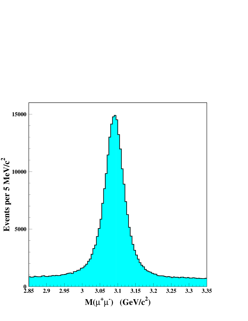
FIG. 1.: The distribution of $\mu^{+}\mu^{-}$ masses. The data used for further analysis lie between 3.047 and 3.147 GeV/$c^{2}$ and contain $196,000\pm 500$ $J/\psi$ events above a background continuum of $20,000\pm 150$ events under the $J/\psi$ peak.

FIG. 2.: The distribution of masses of $J/\psi\,K^{\pm}$ candidates. The solid curve represents a least squares fit to the data between 5.15 and 5.8 GeV/$c^{2}$ consisting of a Gaussian signal above a linear background. The area of the Gaussian contribution is $290\pm 19$ events.

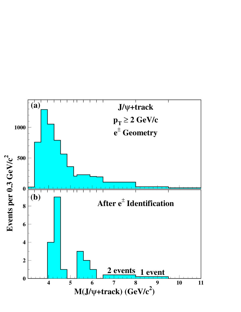
FIG. 3.: Histograms of the number of events vs. M($J/\psi$ + track). (a) $J/\psi\,e$ candidates. For the 6530 events in this histogram, we assigned the electron mass to the third track and required  $p_{T}\geq 2.0$ GeV/$c$. We applied the geometric criteria but not the particle identification criteria for electrons. (b) The 23-event subset of the distribution above that satisfies the electron identification criteria. Note that the bins in $M$($J/\psi$ + track) are not uniform in width. The bin boundaries are indicated by tick marks at the top of the figures here and in subsequent mass histograms. The binning is discussed in the text.

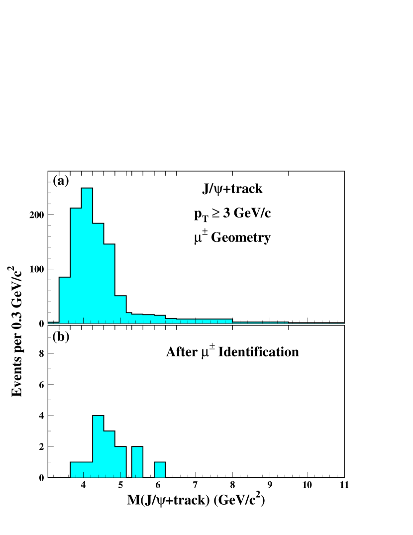
FIG. 4.: Histograms of the number of events vs. M($J/\psi$ + track). (a) $J/\psi\,\mu$ candidates. For the 1055 events in this histogram, we assigned the muon mass to the third track and required  $p_{T}\geq 3.0$ GeV/$c$. We applied the geometric criteria but not the particle identification criteria for muons. (b) The 14-event subset from (a) that satisfies the muon identification criteria.

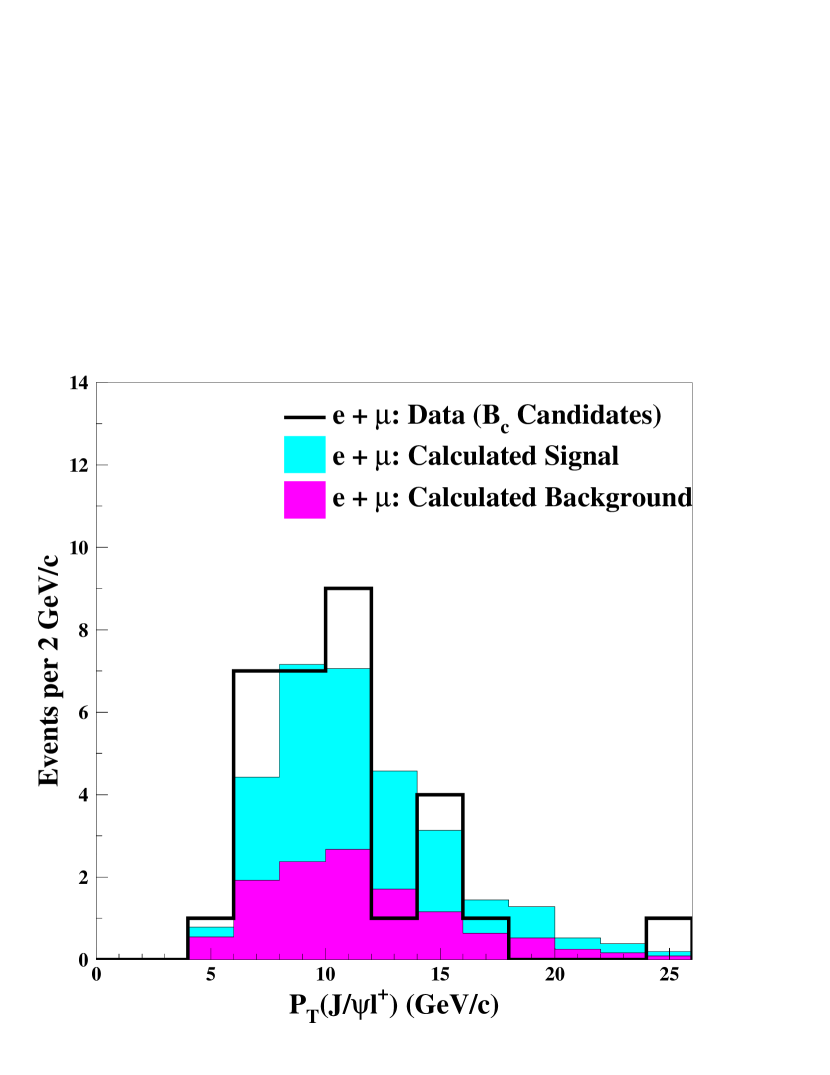
FIG. 5.: The transverse-momentum distribution for the $J/\psi\,\ell$ system in $B_{c}$ candidates (line). It is compared with the normalized $p_{T}$ distribution for all backgrounds (dark shading) and with the $p_{T}$ distribution for $B_{c}\rightarrow J/\psi\,\ell\,\nu$ events generated by Monte Carlo calculations (light shading). The latter is normalized to the fitted number of $B_{c}$ events determined in Sec. V.

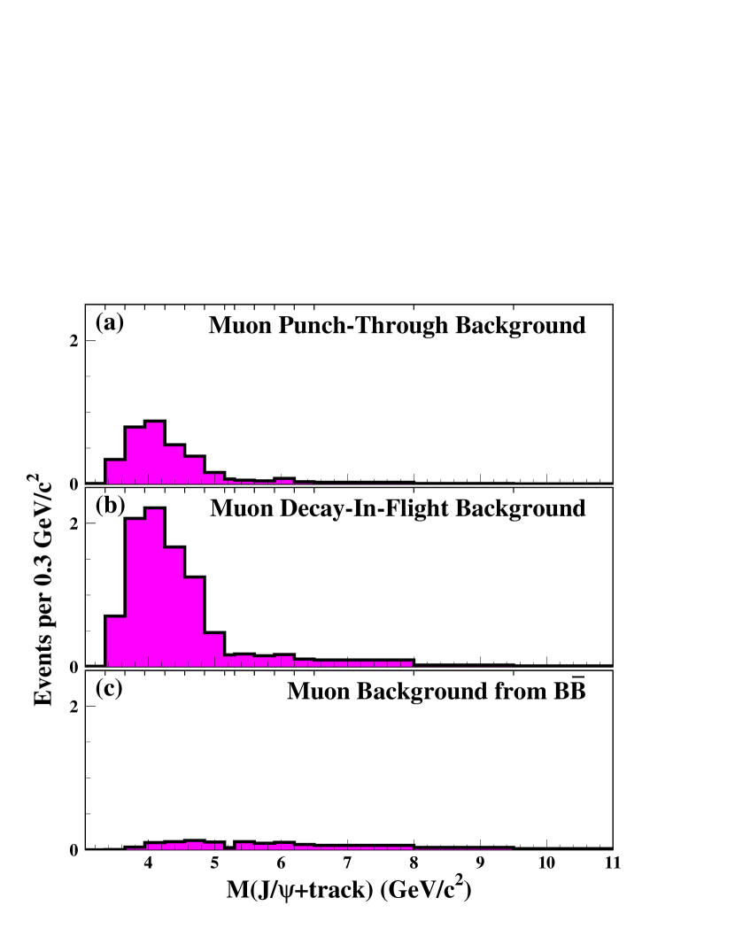
FIG. 6.: Mass histograms for backgrounds from hadrons misidentified as muons. (a) The sum of punch-through background contributions from $\pi^{\pm}$, $K^{+}$ and $K^{-}$. The dominant contribution to the punch-through background is from $K^{+}$ because of its lower interaction cross section. (b) The sum of decay-in-flight background contributions from $\pi^{\pm}$ and $K^{\pm}$. (c) The contribution from $B\overline{B}$ background. These plots are normalized by their calculated contribution to the candidate distribution in Fig. 4.

FIG. 7.: (a) and (b) show the $p_{T}$-dependent probability for kaons and pions, respectively, to decay in flight and be misidentified as muons. The specific ionization $dE/dx$ was used to determine the correct proportion of pions and kaons in the data.

FIG. 8.: The probability of incorrectly identifying a hadron as an electron as a function of $p_{T}$. Tracks from both the JET20 sample and minimum bias sample were used (App. B). (a) and (b) show the data for the isolation parameter $I<0.2$ and $I>0.2$, respectively. The probability averaged over the third-track momentum spectrum for the events in Fig. 3a is $(0.066\pm 0.006)$%.

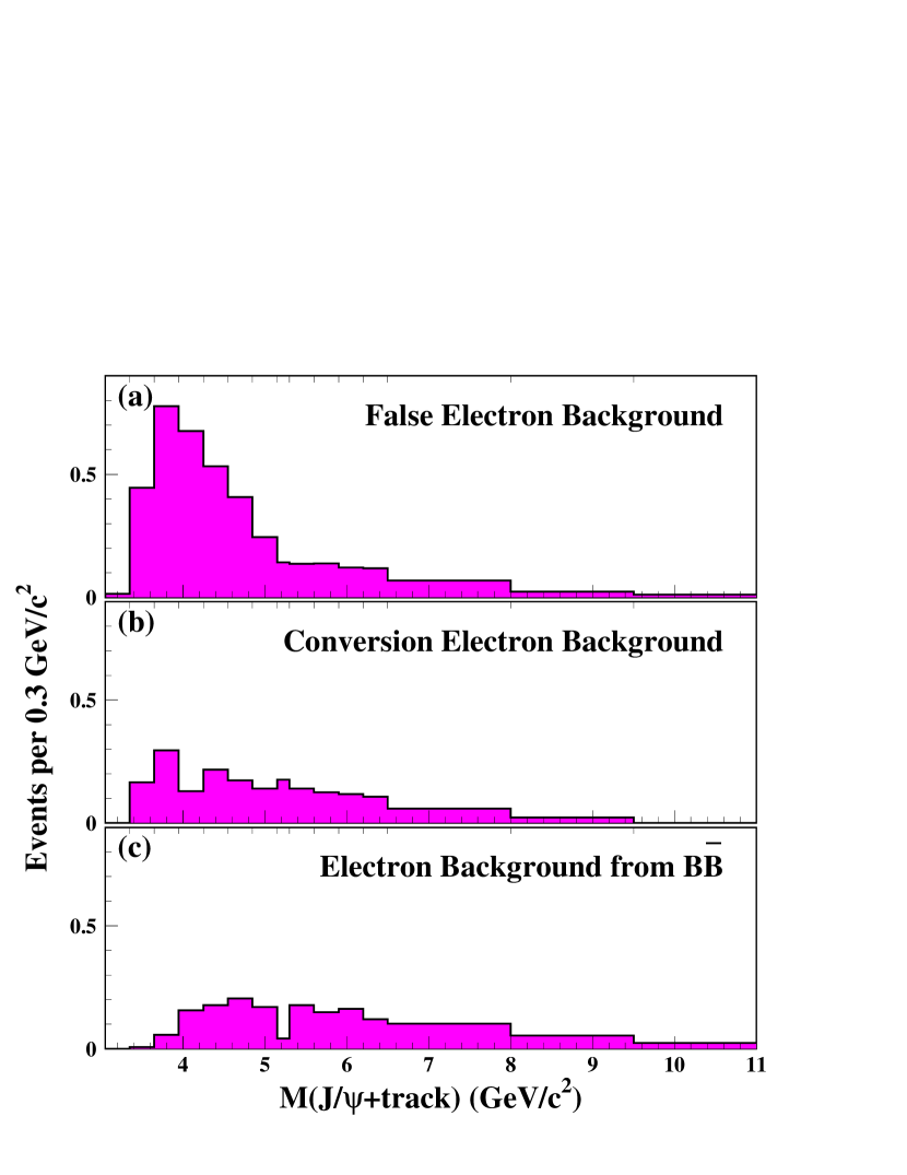
FIG. 9.: The $J/\psi\,e$ mass distribution (a) for background events resulting from misidentified electrons. (b) For events in which the electron originated from a $\gamma$ conversion or Dalitz decay that was not identified as such. (c) For $B\overline{B}$ events in which the $J/\psi$ came from one parent and the electron from another. These plots are normalized by their expected contribution to the candidate distribution in Fig. 3.

FIG. 10.: The difference in $dE/dx$ observed for the third track in $J/\psi$ + track events and that expected for an electron. For electrons, $Q$ has a mean of $Q_{e}$ and a standard deviation of $\sigma_{Q}$. We scaled the difference to yield a distribution with zero mean and unit standard deviation for a pure sample of electrons. (a) The same events shown in Fig. 3(a), where we assigned the electron mass to thethird track, required $p_{T}>2.0$ GeV/$c$, and applied the geometric criteria, but not the particle identification criteria for electrons. (b) The subset of the distribution above that satisfy all the electron identification criteria except $dE/dx$.

FIG. 11.: Conversion Background. (a) The momentum spectrum for the track from an electron-positron pair that fulfilled the requirements for the third lepton and (b) the momentum spectrum for the other member of the pair. To obtain a larger data sample, we removed the requirements on $ct^{\ast}$ and $P(\chi^{2})$ for the vertex fit. In both (a) and (b) the data distributions are normalized to unit area. The Monte Carlo distributions are normalized to the data for $p_{T}$ $>0.5$ GeV/$c^{2}$. In the lowest bin in (b), the difference between data and Monte Carlo arises from the dropoff in track reconstruction efficiency for $p_{T}$ $<0.5$ GeV/$c$. This is the reason for the undetected conversion background.

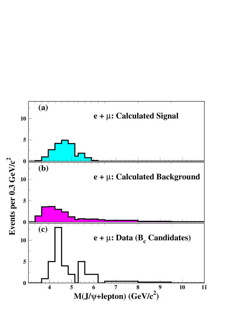
FIG. 12.: (a) A tri-lepton mass distribution for $B_{c}\rightarrow J/\psi\,\ell\,\nu$ based on Monte Carlo calculations. It is normalized to the fitted number of $B_{c}$ events. The distribution was generated under the assumption that the mass of the $B_{c}$ is 6.27 GeV/$c^{2}$. There are negligible differences between the shapes for $B_{c}\rightarrow J/\psi\,\mu$ and $B_{c}\rightarrow J/\psi\,e$. Note that ($93.0\pm 0.6$)% of the area falls in the signal region 4.0–6.0 GeV/$c^{2}$. (b) The normalized mass distribution for all backgrounds for both muon and electron channels. (c) The mass distribution for $B_{c}$ candidates in the data for both muon and electron channels. Note that each of these is a summary histogram, i.e. the sum of several individual histograms presented earlier. We emphasize that the fitting procedures use the full information from individual distributions rather than the sums.

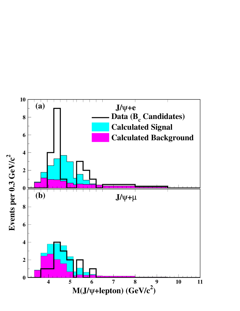
FIG. 13.: Histograms of the $J/\psi\,\ell$ mass that compare the signal and background contributions determined in the likelihood fit to (a) the data for $J/\psi\,e$ and (b) the data for $J/\psi\,\mu$. Note that the mass bins vary in width.

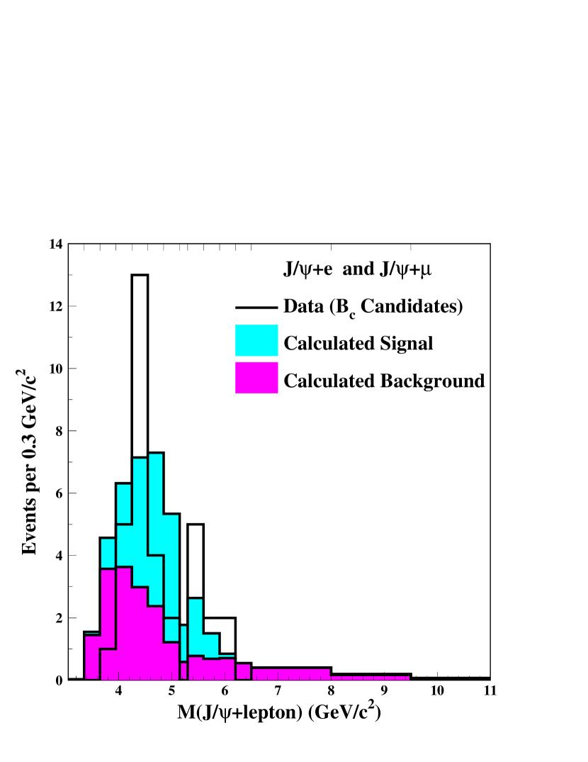
FIG. 14.: Histogram of the $J/\psi\,\ell$  mass that compare the signal and background contributions determined in the likelihood fit to the combined data for $J/\psi\,e$ and $J/\psi\,\mu$. Note that the mass bins vary in width. The total $B_{c}$ contribution is $20.4^{+6.2}_{-5.5}$ events.

FIG. 15.: The variation of $\xi^{2}=-2\ln{(\cal L/L_{\rm 0})}$ as a function of the number of $B_{c}$ mesons. For each fixed value of $N(B_{c})$ all other parameters were adjusted for the best fit. We find $N(B_{c})=20.4^{+6.2}_{-5.5}$ at the minimum.

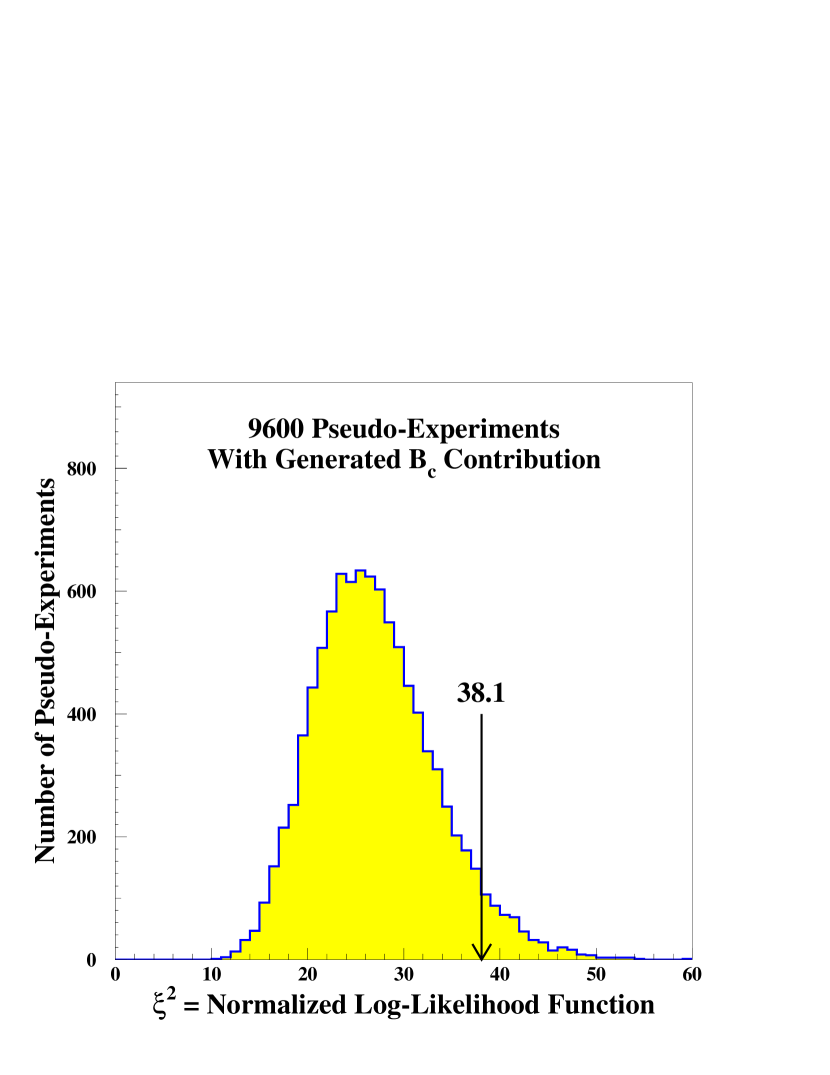
FIG. 16.: Each entry in this histogram is the result of a fit to a Monte Carlo pseudo-experiment that simulated the statistical properties of our data. The backgrounds were generated with the measured means and varied using Poisson or Gaussian statistics as appropriate. $B_{c}$ events were included with statistical fluctuations from the mean of 20.4 and bin-by-bin fluctuations. The resulting muon and electron events were fit as with the data. The values of $\xi^{2}$ are histogrammed here and compared with the value found for the experimental data.

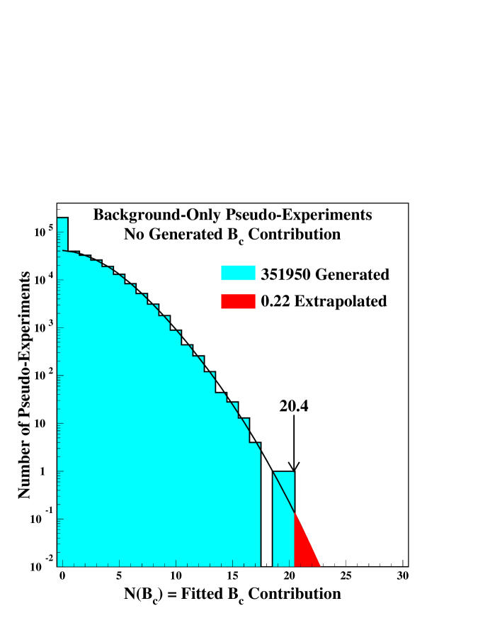
FIG. 17.: Each entry in this histogram is the result of a fit to a Monte Carlo simulation of the statistical properties of this experiment. We generated the backgrounds randomly according to the measured means and varied using Poisson or Gaussian statistics as appropriate. The $B_{c}$ contribution was set to zero in generating the distribution. We then fit the resulting numbers of muon and electron events using the likelihood function. The fitting function included a $B_{c}$ contribution. The histogram above is a measure of the probability of finding a false $B_{c}$ contribution of size $N(B_{c})$ where none exists. Upward and downward fluctuations of the generated samples can require both positive and negative solutions for $N(B_{c})$. We chose to collect all negative solutions in the lowest bin in this figure where these events produce a prominent excess. The smooth curve represents a fit of a convenient extrapolation function (the sum of two Gaussians) to estimate the area beyond 20.4 events.

FIG. 18.: Templates used to determine the quality of the fit to the mass spectrum for various assumed values of the $B_{c}$ mass. Of the 11 values used, four templates are shown here for the following values of $M(B_{c})$: (a) $5.52$ GeV/$c^{2}$, (b) $6.27$ GeV/$c^{2}$, (c) $7.27$ GeV/$c^{2}$, and (d) $7.52$ GeV/$c^{2}$. In each case the histogram displays the binned results of the Monte Carlo calculation and the smooth curve is a spline fit to the histogram.

FIG. 19.: (a) The relative log-likelihood function $\xi^{2}_{m}$ from fits to the data for various values of the assumed mass of the $B_{c}$. Error bars on $\xi^{2}_{m}$ represent its fluctuations with different Monte Carlo samples of $B_{c}$ events at the same mass. The parabolic curve is a fit to the plotted points with $\chi^{2}/n_{d.o.f.}=4.3/8$. A horizontal line is drawn through the parabola’s minimum which occurs at $M(B_{c})=6.40$ GeV/$c^{2}$. Another line one unit above its minimum indicates the one-standard-deviation uncertainties of $\pm 0.39$ GeV/$c^{2}$. (b) The fitted number of $B_{c}$ events vs. $M(B_{c})$. It is stable over the range of theoretical predictions for $M(B_{c})$, 6.1 to 6.5 GeV/$c^{2}$.

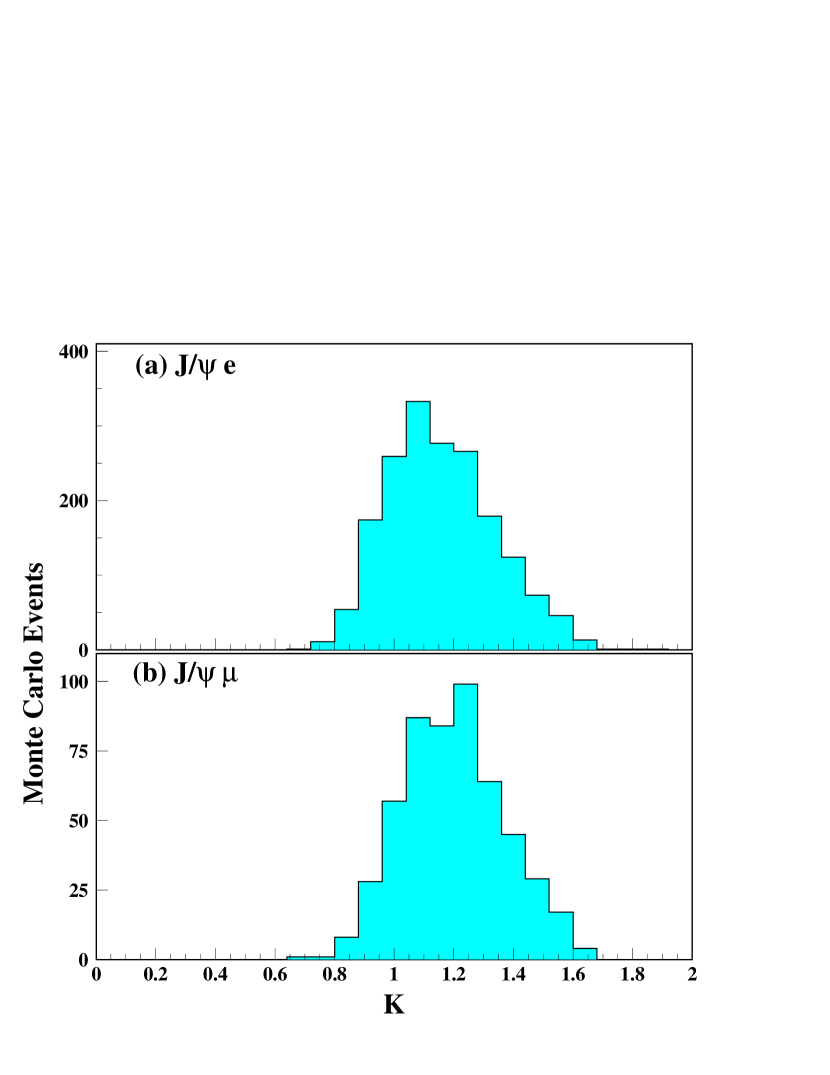
FIG. 20.: $K=(M(B_{c})/p_{T}(B_{c})/(M(J/\psi\,\ell)/p_{T}(J/\psi\,\ell))$ distribution using Monte Carlo simulation (a) for the electron channel and (b) for the muon channel.

FIG. 21.: Pseudo-proper decay length distributions for the background distributions. (a) $J/\psi\,e$ background from false electrons. (b) $J/\psi\,e$ background from conversion electrons. (c) $J/\psi\,\mu$ background from false muons. (d) $B\overline{B}$ background. Its shape is the same for both $J/\psi\,e$ and $J/\psi\,\mu$.

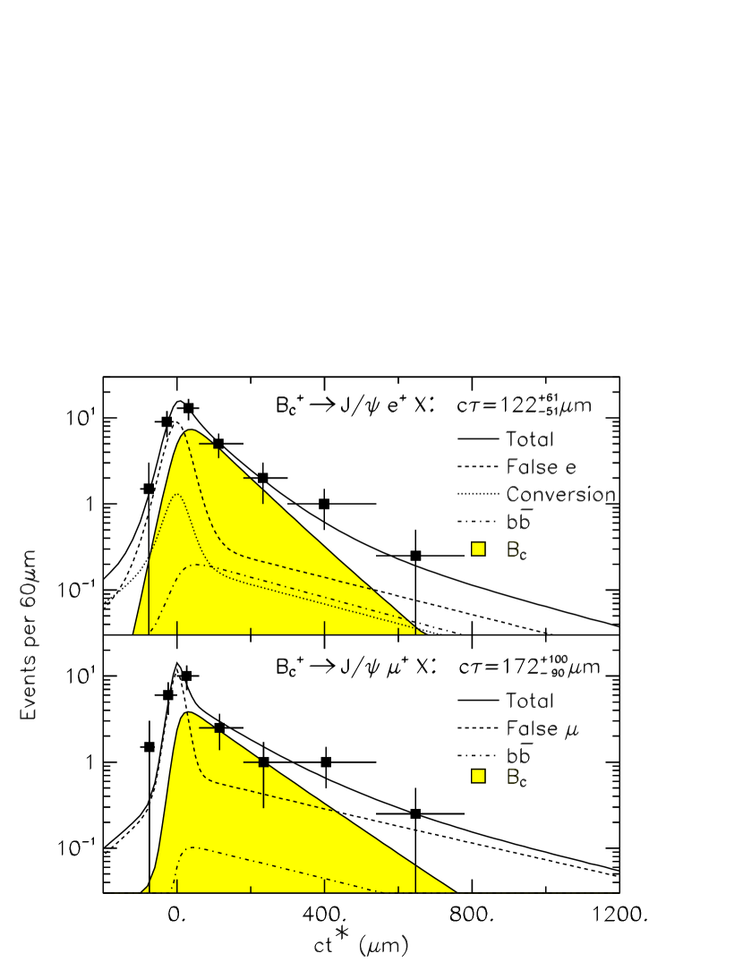
FIG. 22.: Pseudo-proper decay length distributions for data with the fitted curve and the contributions from backgrounds (a) for the electron channel and (b) the muon channel.

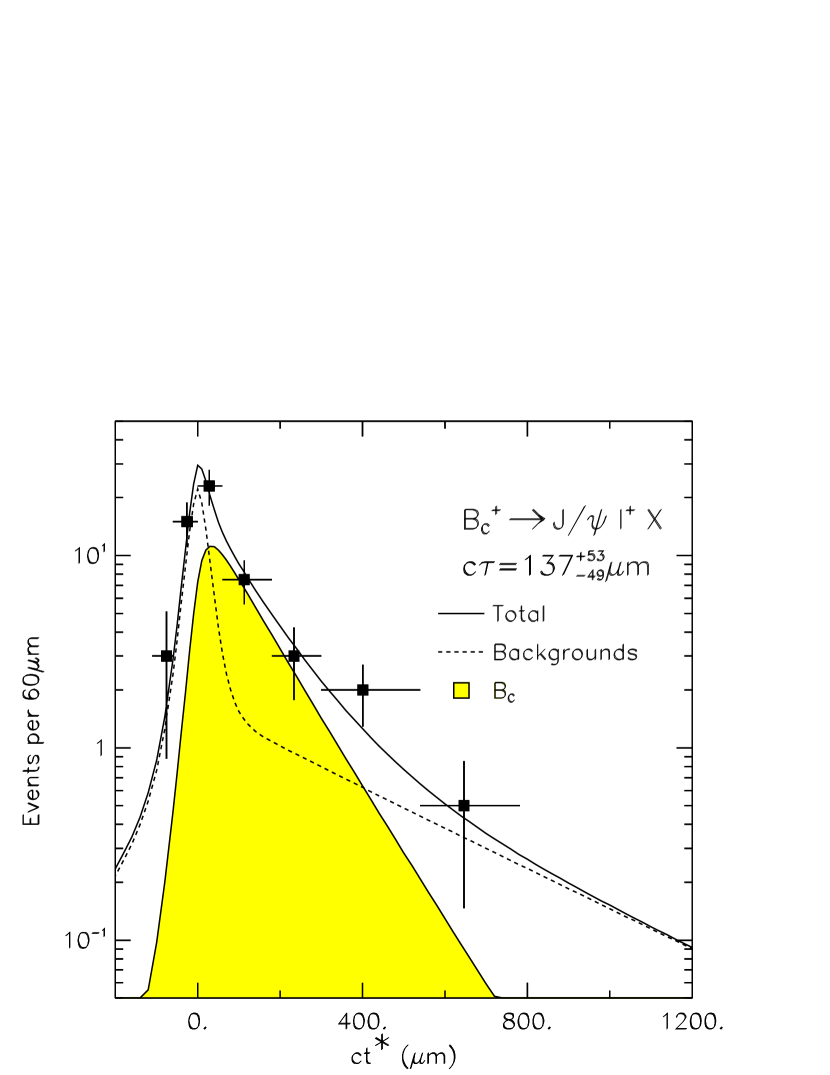
FIG. 23.: Pseudo-proper decay length distribution for the combined $J/\psi\,\mu$ and $J/\psi\,e$ data along with the fitted curve and contributions to it from signal and background

FIG. 24.: The change in $-2\ln({\cal L})$ from its minimum as a function of $c\tau$ for the fit to the $ct^{\ast}$ distribution of $B_{c}$ candidates.

FIG. 25.: Results from 500 pseudo-experiments to simulate the statistics in the $B_{c}$ lifetime analysis: (a) $-2\ln{\cal L}$; (b) fitted lifetime; (c) solid (dashed) line for the negative (positive) uncertainty; (d) ($c\tau_{fit}$ $-$ $c\tau_{input}$)/$\sigma_{fit}$. In (d), the positive (negative) uncertanty was used when the fitted lifetime was smaller (larger) than the input lifetime.

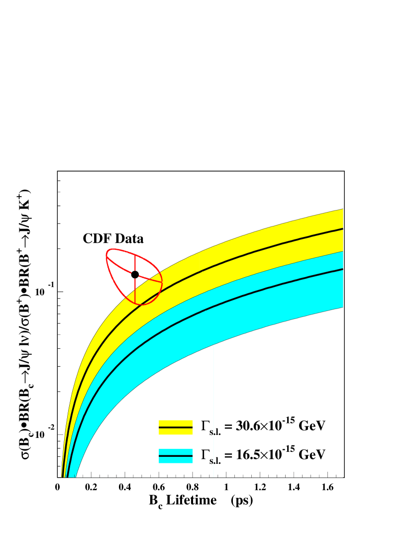
FIG. 26.: The point with 1-standard-deviation contour shows our measured value of the ratio $\sigma\cdot BR(B_{c}^{+}\to J/\psi\;l^{+}X)/\sigma\cdot BR(B^{+}\to J/\psi K^{+})$ plotted at the value we measure for the $B_{c}$ lifetime. The shaded region represents theoretical predictions and their uncertainty corridors for two different values of the semileptonic width $\Gamma_{s.l.}$ based on Refs. [1] and [3]. The other numbers assumed in the theoretical predictions are discussed in the text.

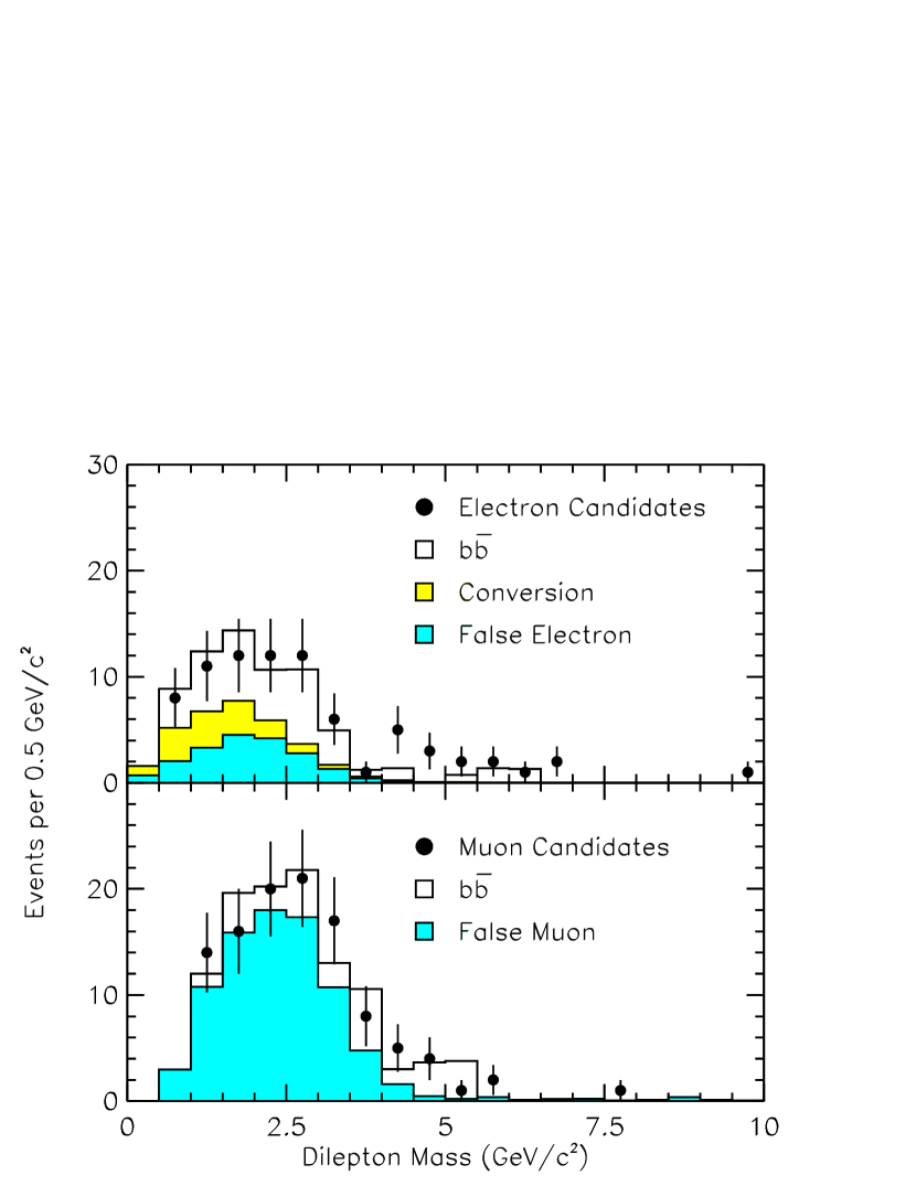
FIG. 27.: Same-charge di-lepton mass distributions for a trigger lepton and a tagged lepton. Both were required to come from a displaced vertex and be within the same jet cone. In (a) the tagged lepton is an electron, and in (b) the tagged lepton is a muon. In both cases, the data from trigger electrons and that from trigger muons are combined. The points with uncertainties are data, and the histograms show the predicted contributions from the various backgrounds relevant to the $B_{c}$ analysis.

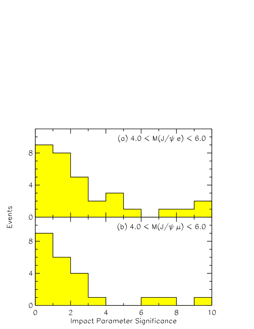
FIG. 28.: (a) Distribution of the impact parameter significance of the third track with respect to the $J/\psi$ vertex for $J/\psi\,e$ events. (b) The same distribution for the $J/\psi\,\mu$ events.

REFERENCES

- [1] M. Lusignoli and M. Masetti, Z. Phys. C 51, 549 (1991).
- [2] N. Isgur, D. Scora, B. Grinstein, M. B. Wise, Phys. Rev. D 39, 799 (1989).
- [3] D. Scora and N. Isgur, Phys. Rev. D 52, 2783 (1995).
- [4] C. H. Chang and Y. Q. Chen, Phys. Rev. D 49, 3399 (1994).
- [5] W. Kwong and J. Rosner, Phys. Rev. D 44, 212 (1991).
- [6] E. Eichten and C. Quigg, Phys. Rev. D 49, 5845 (1994).
- [7] I. I. Bigi, Phys. Lett. 371B, 105 (1996).
- [8] M. Beneke and G. Buchalla, Phys. Rev. D 53, 4991 (1996).
- [9] S. S. Gershtein et al., Int. J. Mod. Phys. A6, 2309 (1991).
- [10] P. Colangelo et al., Z. Phys. C 57, 43 (1993).
- [11] C. Quigg, Proceedings of the Workshop on B Physics at Hadron Accelerators, ed. by P. McBride and C. Shekhar Mishra, Fermilab-CONF-93/267 (SSCL-SR-1225) (1994).
- [12] Myoung-Taek Choi and Jae Kwan Kim, Phys. Rev. D 53, 6670 (1996).
- [13] M. Lusignoli, M. Masetti and S. Petrarca, Phys. Lett. B 266, 142 (1991).
- [14] E. Braaten, K. Cheung and T. C. Yuan, Phys. Rev. D 48, R5049 (1993).
- [15] C. H. Chang and Y. Q. Chen, Phys. Rev. D 48, 4086 (1993).
- [16] C. H. Chang, Y. Q. Chen and R. J. Oakes, Phys. Rev. D 54, 4344 (1996).
- [17] M. Masetti and F. Sartogo, Phys. Lett. 357B, 659 (1995).
- [18] P. Abreu et al., The DELPHI Collaboration, Phys. Lett. 398B, 207 (1997).
- [19] K. Ackerstaff et al., The OPAL Collaboration, CERN Preprint CERN-PPE/97-137, (submitted to Phys. Lett. B).
- [20] R. Barate et al., The ALEPH Collaboration, Phys. Lett. 402B, 213 (1997).
- [21] F. Abe et al., The CDF Collaboration, Phys. Rev. Lett. 77, 5176 (1996).
- [22] For details on the backgrounds and several aspects of the analysis of the channel see J. Suzuki, “Observation of the Meson in 1.8-TeV Proton-Antiproton Collisions”, Ph.D. Dissertation, University of Tsukuba, 1998.
- [23] For details on the backgrounds and several aspects of the analysis of the channel see Prem P. Singh, “Search for the Meson at CDF”, Ph.D. Dissertation, University of Pittsburgh, 1997.
- [24] F. Abe et al., The CDF Collaboration, Nucl. Instrum. Methods Phys. Res. Sect. A 271, 387 (1988).
- [25] F. Abe et al., The CDF Collaboration, Phys. Rev. D 50, 2966 (1994). Section 5.3 of this paper gives details of the electron and muon identification procedures similar to those used in the present analysis.
- [26] D. Amidei et al., Nucl. Instrum. Methods Phys. Res. Sect. A 350, 73 (1994).
- [27] P. Azzi et al., Nucl. Instrum. Methods Phys. Res. Sect. A 360, 137 (1995).
- [28] Prompt signals from the CTC were sent to a fast track processor to provide measurements of track momenta with resolution . For details, see G. W. Foster et al., Nucl. Instrum. Methods Phys. Res. Sect. A 269, 93 (1988).
- [29] reconstruction in this analysis followed well established CDF procedures which have been reported elsewhere. See, e.g. F. Abe et al., The CDF Collaboration, Submitted to Phys. Rev. D, Fermilab-Pub-97/352-E (1997).
- [30] “Review of Particle Physics,” R. M. Barnett et al., Phys. Rev. D 54, 1 (1996).
- [31] M. L. Mangano, P. Nason and G. Ridolfi, Nucl Phys. B 373, 295 (1992).
- [32] P. Nason, S. Dawson and R. K. Ellis, Nucl. Phys. B 303, 607 (1988); Nucl. Phys. B 327, 49 (1989); Erratum 335, 260 (1990).
- [33] A. D. Martin, R. G. Roberts and W. J. Stirling, Phys. Lett. 306B, 145 (1993).
- [34] James Bott et al., Phys. Lett. B304, 159 (1993).
- [35] P. Avery, K. Read and G. Trahern, Cornell Internal Note CSN-212, 1985 (unpublished).
- [36] “Semileptonic Hadron Decay in the Quark Potential Model”, D. J. Scora, Ph.D. Dissertation, University of Toronto, (1992).
- [37] C. Peterson et al., Phys. Rev. D 27, 105 (1983).
- [38] J. Chrin, Z. Phys. C 36, 163 (1987).
- [39] F. Abe et al., The CDF Collaboration, Phys. Rev. D 45, 1448 (1992).
- [40] J.D. Richman and P.R. Burchat, Rev. Mod. Phys. 67, 893 (1995).