First observation of five charmless hadronic $B$ decays

Abstract

There has been much progress in measurements of charmless hadronic $B$ decays during 1997. Building on the previous indications from CLEO and LEP, CLEO now has clear signals in five exclusive final states: $K^{+}\pi^{-}$, $K^{0}\pi^{+}$, ${\eta^{\prime}}K^{+}$, ${\eta^{\prime}}K^{0}$, and $\omega K^{+}$. The branching fractions for the ${\eta^{\prime}}K$ modes are several times larger than the others. A similar strikingly large signal has been seen in the inclusive decay, $B\rightarrow{\eta^{\prime}}X_{S}$. All of these signals would appear to be dominated by hadronic penguin processes.

I Introduction

Charmless hadronic $B$ decays are expected to proceed primarily through $b\rightarrow s$ loop (“penguin”) diagrams and $b\rightarrow u$ spectator diagrams. In Fig. 1 we show four such diagrams for three of the $K\pi$ modes discussed in this paper. We also show the diagrams expected to dominate the final states with an isoscalar meson and a $K$ or $K^{*}$ meson. Interchange of $d$ and $u$ spectator quarks will generally provide the diagrams for both $B^{+}$ and $B^{0}$ decays. Diagrams 1c, 1d, and 1g are Cabibbo suppressed. The un-suppressed versions of these diagrams and the CKM [1] suppressed versions of the penguin diagrams lead to final states such as $\pi\pi$, ${\eta^{\prime}}\pi$, $\eta\rho$, and $\omega\pi$.

These decays have received a great deal of attention because interference among penguin and spectator diagrams leading to the same final state can produce (direct) $CP$ violation, and, for the $B^{0}$ system, interference between final states reached directly or via $B$-$\bar{B}$ mixing, can generate (indirect) $CP$ violation [2]. Detectors such as B$\scriptstyle\sl A$B$\scriptstyle\sl AR$, Belle or others at hadron colliders will attempt to measure an oscillation in the time evolution of certain $B^{0}$ decays, which is sensitive to the value of some of the CKM angles. Other approaches have been suggested [3] notably the possibility of using “quadrangle” relations [4] among amplitudes of four related decays to determine CKM angles.

In subsequent sections, we will review the experimental situation prior to 1997 and then report the results of several new analyses from CLEO which have found the first unambiguous evidence for individual charmless hadronic $B$ decays. We conclude with interpretations of these results.

II Previously published results

Until this year, there have been relatively few indications of charmless hadronic $B$ decays. CLEO first published evidence for the modes $B^{0}\rightarrow K^{+}\pi^{-}$ and $B^{0}\rightarrow\pi^{+}\pi^{-}$ [5], but due to lack of statistics, was unable to claim a signal for either mode separately. Subsequently CLEO updated these results, still without an observation of either mode individually, and provided limits for many other related modes [6].

At LEP $B$ mesons are produced with high momentum so they travel $\sim$1 mm before decaying. Several LEP experiments have used the excellent vertex resolution provided by their silicon vertex detectors to obtain virtually background-free evidence for charmless hadronic $B$ decays. Examples of such events are shown in Fig. 3 for the ALEPH experiment [7]. The experimental difficulty is that the LEP experiments also cannot separate the decays $B^{0}\rightarrow K^{+}\pi^{-}$ and $B^{0}\rightarrow\pi^{+}\pi^{-}$, or these from $B_{S}\rightarrow K^{+}K^{-}$. Fig. 3 shows the mass distribution for ten candidate charmless hadronic $B$ decays from the DELPHI experiment [8].

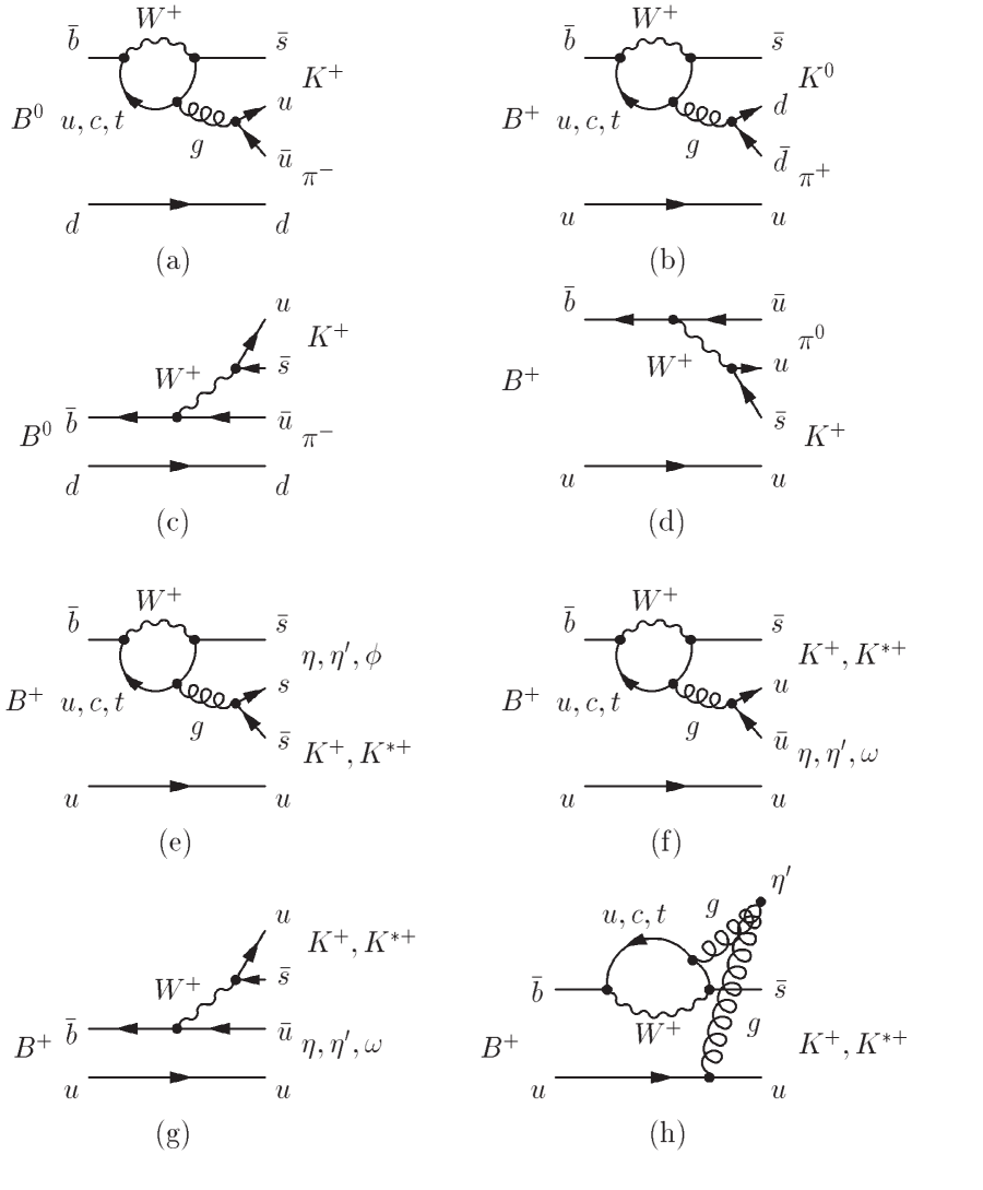
FIG. 1.: Feynman diagrams for some of the penguin and spectator processes which are expected to be dominant for the modes described in this paper.

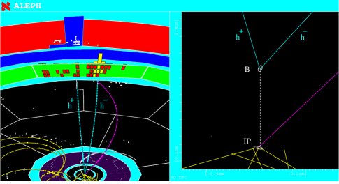
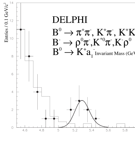
FIG. 2.: Event from the ALEPH experiment showing a $B^{0}\rightarrow K^{+}\pi^{-}$ decay candidate as reconstructed with use of the ALEPH silicon vertex detector.

FIG. 3.: Invariant mass distribution obtained by DELPHI for ten charmless hadronic $B$ decay candidates, background events at lower mass, and the Monte Carlo expectation for the background.

III Results for exclusive decays from CLEO

The results in this section are based on data collected with the CLEO II detector [9] at the Cornell Electron Storage Ring (CESR). The data sample corresponds to an integrated luminosity of 3.11 fb^-1 taken on the $\Upsilon$(4S) resonance and 1.61 fb^-1 taken slightly below. The on-resonance data sample contains $3.3\times 10^{6}$ $B\overline{B}$ pairs. Resonance states are reconstructed from charged tracks and photons with the decay channels: ${\eta^{\prime}}\rightarrow\eta\pi^{+}\pi^{-}$, ${\eta^{\prime}}\rightarrow\rho^{0}\gamma$, $K^{0}$ via $K_{S}\rightarrow\pi^{+}\pi^{-}$, $\rho^{0}\rightarrow\pi^{+}\pi^{-}$, $\pi^{0}\rightarrow\gamma\gamma$, $\eta\rightarrow{\gamma\gamma}$, $\eta\rightarrow\pi^{+}\pi^{-}\pi^{0}$, $\omega\rightarrow\pi^{+}\pi^{-}\pi^{0}$, $\phi\rightarrow K^{+}K^{-}$, $K^{*0}\rightarrow K^{+}\pi^{-}$, $K^{*0}\rightarrow K^{0}\pi^{0}$, $K^{*+}\rightarrow K^{+}\pi^{0}$, and $K^{*+}\rightarrow K^{0}\pi^{+}$. Charge conjugate decays are implied throughout this paper.

Candidate charged tracks are required to pass quality cuts and have specific ionization ($dE/dx$) consistent with that of a pion and kaon. Such tracks must not be electrons or muons, identified by calorimetry and depth of penetration of an iron muon stack, respectively. $K_{S}\rightarrow\pi^{+}\pi^{-}$ candidates are accepted only if they are displaced from the primary interaction point by at least $3$ mm. Photon candidates are isolated calorimeter showers with a measured energy of at least 30 (50) MeV in the central (end cap) region of the calorimeter. The momentum of charged tracks and photon pairs is required to be greater than 100 MeV/c to reduce combinatoric background. Photon pairs and vees are fit kinematically to the appropriate combined mass hypothesis to obtain the meson momentum vectors. Resolutions on the reconstructed masses prior to the constraint are about 5-10 MeV for $\pi^{0}\rightarrow{\gamma\gamma}$, 12 MeV for $\eta_{{\gamma\gamma}}$, and 3 MeV for $K_{S}\rightarrow\pi^{+}\pi^{-}$.

The primary means of identification of $B$ meson candidates is through their measured mass and energy. The resolution for $\Delta E\equiv E_{1}+E_{2}-E_{b}$ ($E_{1}$ and $E_{2}$ are the energy of the two daughter particles of the $B$ and $E_{b}$ is the beam energy) is typically 25-50 MeV. The resolution for $M\equiv\sqrt{E_{b}^{2}-{\bf p}_{B}^{2}}$ (${\bf p}_{B}$ is the reconstructed $B$ momentum) is 2.5-3.0 MeV, dominated by the uncertainty in ${\bf p}_{B}$. Signals are identified with the use of resonance masses and, in the case of vector-pseudoscalar decays and the ${\eta^{\prime}}\rightarrow\rho^{0}\gamma$ channel, a variable ${\cal H}$ sensitive to the helicity distribution of the decay. For modes in which one daughter is a single charged track, or is a resonance pairing a charged track with a $\pi^{0}$, the $dE/dx$ variables $S_{K}$ and $S_{\pi}$ are used. The latter are defined as the deviations from nominal energy loss for the indicated particle hypotheses measured in standard deviations. Studies of $D^{*+}$ tagged $D^{0}\rightarrow K^{-}\pi^{+}$ decays find a $K$-$\pi$ separation of about 1.7 standard deviations near 2.5 GeV/c.

The large background from continuum quark production ($e^{+}e^{-}\rightarrow q\bar{q}$) can be reduced with the use of event shape cuts. One such cut involves the quantity $\theta_{BB}$, the angle between the thrust axis of the candidate $B$ and that of the rest of the event (sphericity is used instead of thrust for the $K\pi$ and $\pi\pi$ analyses). Since $B$ mesons are produced nearly at rest, there is little correlation between the two thrust axes, while candidates extracted from continuum $q\bar{q}$ events tend to be strongly correlated by the jet-like nature of the events. This difference is exploited by requiring $\left|\cos\theta_{BB}\right|<0.9$. A multivariate discriminant ${\cal F}$ is also employed, with the primary inputs being the energy deposition in nine cones concentric with the thrust or sphericity axis of the candidates tracks. Monte Carlo studies indicate that backgrounds from other $B$ decay modes are small and they are not considered further.

In order to extract event yields, an unbinned extended-maximum-likelihood (ML) fit [10] is performed, which includes sidebands about the expected mass and energy peaks, of a superposition of expected signal and background distributions:

$${\cal L} = e^{-(N_{S}+N_{B})}\prod_{i=1}^{N}\{N_{S}{\cal P}_{S_{i}}(f_{1},...,f_{m};x_{1},...x_{p})+N_{B}{\cal P}_{B_{i}}(g_{1},...,g_{m};x_{1},...x_{p})\},$$

where ${\cal P}_{S_{i}}$ and ${\cal P}_{B_{i}}$ are the probabilities for event $i$ to be signal and continuum background, respectively. The probabilities are a function of the values of the variables $x$ used in the fit for each event, and of the parameters $f$ and $g$ used to describe the signal and background shapes for each variable. The variables used are $\Delta E$, $M$, ${\cal F}$, and, where applicable, resonance masses, ${\cal H}$, $S_{K}$, and $S_{\pi}$. $N_{S}$ and $N_{B}$, the free parameters of the fit, are the (positive-definite) number of signal and continuum background events in the fitted data sample, respectively. Sample sizes for these fits range from $\sim 30$ to about ten thousand events.

The signal probability distribution functions (PDFs) $\cal P_{S}$ and $\cal P_{B}$ are constructed as products of functions of the observables ${\bf x}_{i}$; they are determined from fits to Monte Carlo events that simulate the response of the CLEO detector to each decay mode investigated. The GEANT [11] based simulation is tuned to reproduce detector resolution and efficiencies for a variety of benchmark processes. The parameters of the background PDFs are determined with similar fits to a sideband region of data defined by $|\Delta E|<0.2$ GeV and $5.2<M<5.27$ GeV/c². The signal shapes used are Gaussian, double Gaussian, and Breit-Wigner as appropriate for $\Delta E$ and mass peaks. For background, resonance masses are fit to the sum of a smooth polynomial and the signal shape, to account for the component of real resonance as well as the combinatoric background. Shapes used for $\Delta E$ and $M$ background are, respectively, a first-degree polynomial and the empirical shape [12] $f(z)\propto z\sqrt{1-z^{2}}\exp{(-\xi(1-z^{2}))}$, where $z\equiv M/E_{b}$ and $\xi$ is a parameter to be fit. Finally, for ${\cal F}$, $S_{K}$, and $S_{\pi}$, bifurcated Gaussians are used for both signal and background.

TABLE I.: Experimental results and theoretical predictions. Columns list the event yield from the fit, statistical significance, reconstruction efficiency $\epsilon$ (including the branching fraction for the $K^{0}$ via $K_{S}\rightarrow\pi^{+}\pi^{-}$ chain), and the resulting $B$ decay branching fraction ${\cal B}$.

Final	ML fit				Theory
state	events	Signif.	$\epsilon$(%)	$\cal B$($10^{-5})$	$\cal B$($10^{-5})$	References
$\pi^{+}\pi^{-}$	$9.9^{+6.0}_{-5.1}$	2.2$\sigma$	$44\pm 3$	$<~{}1.5$	0.8–1.8	REFERENCES,REFERENCES,REFERENCES,REFERENCES
$\pi^{+}\pi^{0}$	$11.3^{+6.3}_{-5.2}$	2.8$\sigma$	$37\pm 3$	$<~{}2.0$	0.6–2.0	REFERENCES,REFERENCES,REFERENCES,REFERENCES
$\pi^{0}\pi^{0}$	$2.7^{+2.7}_{-1.7}$	2.4$\sigma$	$29\pm 3$	$<0.93$	0.02–0.06	REFERENCES,REFERENCES,REFERENCES,REFERENCES
$K^{+}\pi^{-}$	$21.6^{+6.8}_{-6.0}$	5.6$\sigma$	$44\pm 3$	$1.5^{+0.5}_{-0.4}\pm 0.1$	0.7–2.4	REFERENCES-REFERENCES,REFERENCES,REFERENCES
$K^{+}\pi^{0}$	$8.7^{+5.3}_{-4.2}$	2.7$\sigma$	$37\pm 3$	$<~{}1.6$	0.3–1.3	REFERENCES-REFERENCES,REFERENCES,REFERENCES
$K^{0}\pi^{+}$	$9.2^{+4.3}_{-3.8}$	3.2$\sigma$	$12\pm 1$	$2.3^{+1.1}_{-1.0}\pm 0.4$	0.5–1.3	REFERENCES-REFERENCES,REFERENCES,REFERENCES,REFERENCES
$K^{0}\pi^{0}$	$4.1^{+3.1}_{-2.4}$	2.2$\sigma$	$8\pm 1$	$<~{}4.1$	0.2–0.8	REFERENCES,REFERENCES,REFERENCES,REFERENCES,REFERENCES
$K^{+}K^{-}$	$0.0^{+1.3}_{-0.0}$	0.0$\sigma$	$44\pm 3$	$<~{}0.43$	–
$K^{+}\bar{K}^{0}$	$0.6^{+3.8}_{-0.6}$	0.2$\sigma$	$12\pm 1$	$<~{}2.1$	0.06–0.24	REFERENCES,REFERENCES,REFERENCES,REFERENCES,REFERENCES
$K^{0}\bar{K}^{0}$	0	–	$5\pm 1$	$<~{}1.7$	0.06–0.13	REFERENCES,REFERENCES,REFERENCES,REFERENCES
$h^{+}\pi^{0}$	$20.0^{+6.8}_{-5.9}$	5.5$\sigma$	$37\pm 3$	$1.6^{+0.6}_{-0.5}\pm 0.4$	–

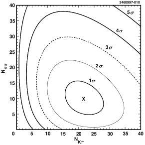
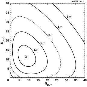
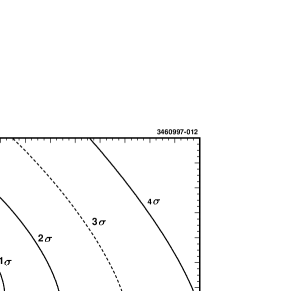
FIG. 4.: Likelihood contours for ML fits to (a) $N_{K^{\pm}\pi^{\mp}}$ and $N_{\pi^{+}\pi^{-}}$ for $B^{0}\rightarrow K^{+}\pi^{-}$ and $B^{0}\rightarrow\pi^{+}\pi^{-}$; (b) $N_{K\pi^{0}}$ and $N_{\pi\pi^{0}}$ for $B^{+}\rightarrow K^{+}\pi^{0}$ and $B^{+}\rightarrow\pi^{+}\pi^{0}$; (c) $N_{K^{0}_{S}K}$ and $N_{K^{0}_{S}\pi}$ for $B^{+}\rightarrow\bar{K}^{0}K^{+}$ and $B^{+}\rightarrow K^{0}\pi^{+}$.

FIG. 5.: $M$ and $\Delta E$ plots for (a) $B^{0}\rightarrow K^{+}\pi^{-}$, (b) $B^{+}\rightarrow h^{+}\pi^{0}$, and (c) $B^{+}\rightarrow K^{0}\pi^{+}$. The scaled projection of the total likelihood fit (solid curve) and the continuum background component (dotted curve) are overlaid.

The results of these fits are given in a Tables I-VI, each with the signal event yield, the efficiency including secondary branching fractions, and the branching fraction for each mode, given as a central value with statistical and systematic error or as a 90% confidence level upper limit. Table I for the $K\pi$ and $\pi\pi$ final states also contains the statistical significance for the fit to each mode. Systematic errors in yield and efficiency are estimated by variation of the fit parameters and estimation of uncertainties in reconstruction efficiencies and selection requirements. Branching fraction upper limits are obtained by increasing the yield and reducing the efficiency by their systematic errors. In Fig. 5, we show the ML contour for the three cases in Table I with significance greater than three standard deviations. While the significance for the $K^{+}\pi^{0}$ and $\pi^{+}\pi^{0}$ final states are both (barely) below $3\sigma$, there is strong evidence for $h\pi^{0}$, where $h$ indicates a charged $K$ or $\pi$. This is very similar to the case of the $h^{+}h^{-}$ final state several years ago [5]. In Fig. 5, we show projections of the fit onto the $M$ and $\Delta{\rm E}$ axes; cuts have been made on other ML variables in order to better reflect the background near the signal region. Further details can be found in reference REFERENCES.

TABLE II.: Measurement results for ${\eta^{\prime}}$ decay modes. Columns list the final states (with secondary decay modes as subscripts), event yield from the fit, reconstruction efficiency $\epsilon$, total efficiency with secondary branching fractions ${\cal B}_{s}$, and the resulting $B$ decay branching fraction ${\cal B}$.

Final state	Fit events	$\epsilon$(%)	$\epsilon\mbox{$\cal B$}_{s}$(%)	$\cal B$($10^{-5})$
${\eta^{\prime}}_{\eta\pi\pi}K^{+}$	$11.2^{+4.1}_{-3.4}$	30	5.1	$6.7^{+2.5}_{-2.1}\pm 0.8$
${\eta^{\prime}}_{\rho\gamma}K^{+}$	$19.6^{+6.6}_{-5.7}$	28	8.4	$7.0^{+2.4}_{-2.1}\pm 0.9$
${\eta^{\prime}}_{5\pi}K^{+}$	$2.3^{+2.2}_{-1.5}$	17	1.7	$4.2^{+4.0}_{-2.7}\pm 1.4$
${\eta^{\prime}}_{\eta\pi\pi}K^{0}$	$1.4^{+1.7}_{-1.0}$	23	1.4	$3.1^{+3.7}_{-2.1}\pm 0.6$
${\eta^{\prime}}_{\rho\gamma}K^{0}$	$5.7^{+3.7}_{-2.8}$	27	2.8	$6.2^{+4.0}_{-3.0}\pm 1.2$
${\eta^{\prime}}_{\eta\pi\pi}\pi^{+}$	$1.4^{+2.2}_{-1.4}$	30	5.2	$<3.7$
${\eta^{\prime}}_{\rho\gamma}\pi^{+}$	$4.0^{+4.6}_{-3.3}$	29	8.8	$<4.5$
${\eta^{\prime}}_{5\pi}\pi^{+}$	$0.5^{+1.9}_{-0.5}$	18	1.8	$<10.7$
${\eta^{\prime}}_{\eta\pi\pi}\pi^{0}$	$0.0^{+0.5}_{-0.0}$	25	4.3	$<1.8$
${\eta^{\prime}}_{\rho\gamma}\pi^{0}$	$0.0^{+2.0}_{-0.0}$	29	8.7	$<2.2$
${\eta^{\prime}}_{\eta\pi\pi}{\eta^{\prime}}_{\eta\pi\pi}$	$0.0^{+0.5}_{-0.0}$	19	0.6	$<15.2$
${\eta^{\prime}}_{\eta\pi\pi}{\eta^{\prime}}_{\rho\gamma}$	$0.0^{+0.8}_{-0.0}$	19	1.7	$<6.4$
${\eta^{\prime}}_{\eta\pi\pi}\eta_{{\gamma\gamma}}$	$0.0^{+0.5}_{-0.0}$	26	1.8	$<4.6$
${\eta^{\prime}}_{\eta\pi\pi}\eta_{3\pi}$	$0.0^{+0.5}_{-0.0}$	17	0.7	$<12.5$
${\eta^{\prime}}_{\rho\gamma}\eta_{{\gamma\gamma}}$	$5.6^{+4.6}_{-3.6}$	28	3.3	$<13.0$
${\eta^{\prime}}_{\rho\gamma}\eta_{3\pi}$	$0.0^{+0.6}_{-0.0}$	16	1.1	$<9.3$
${\eta^{\prime}}_{\eta\pi\pi}K^{*+}_{K^{+}\pi^{0}}$	$0.0^{+1.0}_{-0.0}$	13	0.7	$<18.$
${\eta^{\prime}}_{\eta\pi\pi}K^{*+}_{K^{0}\pi^{+}}$	$0.0^{+1.6}_{-0.0}$	15	0.6	$<24.$
${\eta^{\prime}}_{\eta\pi\pi}K^{*0}$	$0.0^{+0.7}_{-0.0}$	22	2.5	$<3.9$
${\eta^{\prime}}_{\eta\pi\pi}\rho^{+}$	$0.0^{+0.7}_{-0.0}$	12	2.0	$<5.7$
${\eta^{\prime}}_{\eta\pi\pi}\rho^{0}$	$0.0^{+0.5}_{-0.0}$	22	3.8	$<2.3$

The results of the ML fits for the ${\eta^{\prime}}$ analyses are summarized in Table II. A strong signal for $B^{+}\rightarrow{\eta^{\prime}}K^{+}$ is found in both the ${\eta^{\prime}}\rightarrow\eta\pi^{+}\pi^{-}$ ($5.2\sigma$) and ${\eta^{\prime}}\rightarrow\rho^{0}\gamma$ ($4.8\sigma$) channels. Combining these with evidence from the chain ${\eta^{\prime}}\rightarrow\eta\pi^{+}\pi^{-}$, $\eta\rightarrow\pi^{+}\pi^{-}\pi^{0}$ yields a significance of $7.5\sigma$ as shown in Fig. 7a. All significances given here and below include systematic errors in the yield. These are obtained from a Monte Carlo convolution of the likelihood function with resolution functions (assumed Gaussian) for the parameters, including their most important correlations. Efficiency systematics are included as described above. The combined significance for the $B^{0}\rightarrow{\eta^{\prime}}K^{0}$ decay is $3.8\sigma$ as shown in Fig. 7b. The projection plots for these signals are shown in Fig. 7.

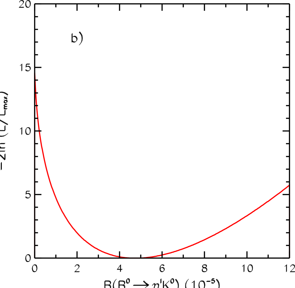
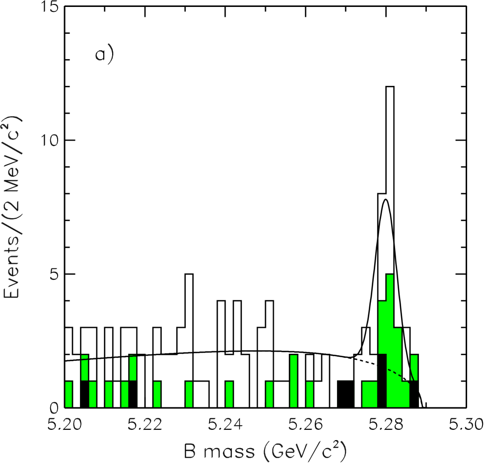
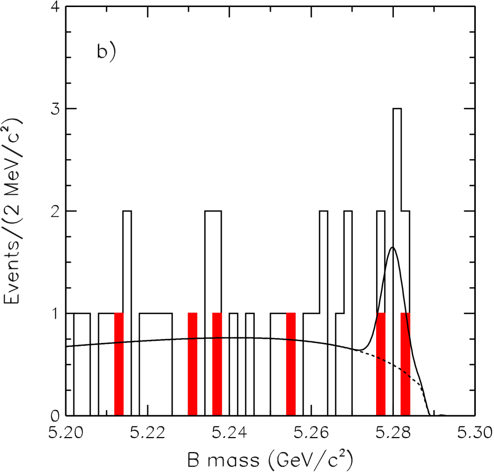
FIG. 6.: (a) Likelihood function contours for $B^{+}\rightarrow\eta^{\prime}h^{+}$; (b) $-2\ln{\mbox{$\cal L$}/\mbox{$\cal L$}_{\rm max}}$ for $B^{0}\rightarrow{\eta^{\prime}}K^{0}$.

FIG. 7.: Projections onto the variable $M$. Overlaid on each plot as smooth curves are the best fit functions (solid) and background components (dashed), calculated with the variables not shown restricted to the neighborhood of expected signal. The histograms show (a) $B^{+}\rightarrow\eta^{\prime}h^{+}$ with $\eta^{\prime}\rightarrow\eta\pi\pi\ (\eta\rightarrow\pi^{+}\pi^{-}\pi^{0}$, dark shaded), $\eta^{\prime}\rightarrow\eta\pi\pi\ (\eta\rightarrow\gamma\gamma$, light shaded), and $\eta^{\prime}\rightarrow\rho\gamma$ (open); (b) ${\eta^{\prime}}K^{0}$ with $\eta^{\prime}\rightarrow\eta\pi\pi$ (shaded) and $\eta^{\prime}\rightarrow\rho\gamma$ (open).

Similarly, the results for the ML fits for the $\eta$ final states are summarized in Table III. Only limits are obtained for these modes, though they are quite restrictive limits in many cases. For final states with multiple secondary channels, the value of $-2\ln{\cal L}$ is summed for each branching fraction bin and the final branching fraction or upper limit s extracted from the combined distribution. Table IV shows the final results for the ${\eta^{\prime}}$ and $\eta$ decay modes, as well as previously published theoretical estimates. Further details concerning the ${\eta^{\prime}}$ and $\eta$ modes can be found in reference REFERENCES.

TABLE III.: Measurement results for $\eta$ decay modes. Columns list the final states (with secondary decay modes as subscripts), event yield from the fit, reconstruction efficiency $\epsilon$, total efficiency with secondary branching fractions ${\cal B}_{s}$, and the resulting $B$ decay branching fraction ${\cal B}$.

Final state	Fit events	$\epsilon$(%)	$\epsilon\mbox{$\cal B$}_{s}$(%)	$\cal B$($10^{-5})$
$\eta_{{\gamma\gamma}}K^{+}$	$1.3^{+3.5}_{-1.3}$	46	17.9	$<1.5$
$\eta_{3\pi}K^{+}$	$0.0^{+2.5}_{-0.0}$	28	6.3	$<3.1$
$\eta_{{\gamma\gamma}}K^{0}$	$1.8^{+2.4}_{-1.6}$	32	4.2	$<4.7$
$\eta_{3\pi}K^{0}$	$0.0^{+0.5}_{-0.0}$	14	1.1	$<8.6$
$\eta_{{\gamma\gamma}}\pi^{+}$	$0.2^{+5.0}_{-0.2}$	47	18.2	$<1.7$
$\eta_{3\pi}\pi^{+}$	$0.0^{+1.8}_{-0.0}$	29	6.6	$<2.6$
$\eta_{{\gamma\gamma}}\pi^{0}$	$0.0^{+0.9}_{-0.0}$	33	13.0	$<0.9$
$\eta_{3\pi}\pi^{0}$	$0.0^{+1.5}_{-0.0}$	23	5.5	$<2.7$
$\eta_{{\gamma\gamma}}\eta_{{\gamma\gamma}}$	$1.1^{+1.7}_{-1.1}$	34	5.2	$<3.0$
$\eta_{{\gamma\gamma}}\eta_{3\pi}$	$0.0^{+1.3}_{-0.0}$	24	4.3	$<2.9$
$\eta_{3\pi}\eta_{3\pi}$	$0.0^{+0.5}_{-0.0}$	16	0.8	$<9.8$
$\eta_{{\gamma\gamma}}K^{*+}_{K^{+}\pi^{0}}$	$0.7^{+3.6}_{-0.7}$	25	3.3	$<8.8$
$\eta_{3\pi}K^{*+}_{K^{+}\pi^{0}}$	$0.0^{+1.2}_{-0.0}$	15	1.2	$<11.7$
$\eta_{{\gamma\gamma}}K^{*+}_{K^{0}\pi^{+}}$	$0.0^{+1.2}_{-0.0}$	24	2.1	$<5.7$
$\eta_{3\pi}K^{*+}_{K^{0}\pi^{+}}$	$0.0^{+1.0}_{-0.0}$	14	0.8	$<16.0$
$\eta_{{\gamma\gamma}}K^{*0}$	$5.2^{+4.0}_{-3.0}$	32	8.4	$<4.6$
$\eta_{3\pi}K^{*0}$	$0.0^{+0.8}_{-0.0}$	20	3.1	$<3.6$
$\eta_{{\gamma\gamma}}\rho^{+}$	$1.2^{+4.1}_{-1.2}$	24	9.9	$<3.3$
$\eta_{3\pi}\rho^{+}$	$2.5^{+4.1}_{-2.5}$	14	3.3	$<11.2$
$\eta_{{\gamma\gamma}}\rho^{0}$	$0.2^{+4.0}_{-0.2}$	36	14.3	$<1.9$
$\eta_{3\pi}\rho^{0}$	$0.0^{+1.1}_{-0.0}$	22	5.1	$<2.7$

TABLE IV.: Combined results for $\eta$ and ${\eta^{\prime}}$ decay modes and expectations from theoretical models.

Decay mode	$\cal B$($10^{-5})$	Theory $\cal B$($10^{-5}$)	References
$B^{+}\rightarrow{\eta^{\prime}}K^{+}$	$6.5^{+1.5}_{-1.4}\pm 0.9$	$0.7-4.1$	[17, 24, 26]
$B^{0}\rightarrow{\eta^{\prime}}K^{0}$	$4.7^{+2.7}_{-2.0}\pm 0.9$	$0.9-3.3$	[17, 26]
$B^{+}\rightarrow{\eta^{\prime}}\pi^{+}$	$<3.1$	$0.8-3.5$	[17, 24, 26]
$B^{0}\rightarrow{\eta^{\prime}}\pi^{0}$	$<1.1$	$0.4-1.4$	[17, 26]
$B\rightarrow{\eta^{\prime}}{\eta^{\prime}}$	$<4.7$	$0.1-2.8$	[17, 26]
$B^{0}\rightarrow{\eta^{\prime}}\eta$	$<2.7$	$0.4-4.4$	[17, 26]
$B^{+}\rightarrow{\eta^{\prime}}K^{*+}$	$<13.$	$0.1-0.9$	[17, 24, 26]
$B^{0}\rightarrow{\eta^{\prime}}K^{*0}$	$<3.9$	$0.8-1.7$	[17, 26]
$B^{+}\rightarrow{\eta^{\prime}}\rho^{+}$	$<4.7$	$0.8-5.7$	[17, 24, 26]
$B\rightarrow{\eta^{\prime}}\rho^{0}$	$<2.3$	$0.2-1.2$	[17, 26]
$B^{+}\rightarrow\eta K^{+}$	$<1.4$	$0.1-0.5$	[17, 24, 26]
$B^{0}\rightarrow\eta K^{0}$	$<3.3$	$0.1-0.2$	[17, 20, 26]
$B^{+}\rightarrow\eta\pi^{+}$	$<1.5$	$0.2-0.8$	[17, 20, 24, 26]
$B^{0}\rightarrow\eta\pi^{0}$	$<0.8$	$0.2-0.4$	[17, 26]
$B^{0}\rightarrow\eta\eta$	$<1.8$	$0.1-1.4$	[17, 20, 26]
$B^{+}\rightarrow\eta K^{*+}$	$<3.0$	$0.1-1.3$	[17, 24, 26]
$B^{0}\rightarrow\eta K^{*0}$	$<3.0$	$0.1-0.5$	[17, 20, 26]
$B^{+}\rightarrow\eta\rho^{+}$	$<3.2$	$0.7-4.4$	[17, 20, 24, 26]
$B^{0}\rightarrow\eta\rho^{0}$	$<1.3$	$0.1-0.8$	[17, 20, 26]

Finally, we give in Table V results for the ML fits for the $\omega$ and $\phi$ final states. Table VI provides a summary of these results, where modes with multiple secondary channels have been combined. A signal with $3.9\sigma$ significance is found for $B^{+}\rightarrow\omega K^{+}$ as shown in Fig. 9a. The corresponding projection plot is shown in Fig. 9a. The significance for the combination of the $\phi K^{*+}$ and $\phi K^{*0}$ final states is marginal - $2.9\sigma$. It is sensible to combine these modes since the penguin diagrams for the $B^{+}$ and $B^{0}$ decays are identical except for the spectator quark and all other processes are expected to be negligible for these decays. If the observed yield is interpreted as a signal, a branching fraction of $(1.1^{+0.6}_{-0.5}\pm 0.2)\times 10^{-5}$ is obtained. The plot of $-2\ln{\cal L}$ and fit projections are shown in Figs. 9b and 9b, respectively. Further details concerning the $\omega$ and $\phi$ modes can be found in reference REFERENCES.

TABLE V.: Measurement results for $\omega$ and $\phi$ decay modes. Columns list the final states (with secondary decay modes as subscripts), event yield from the fit, reconstruction efficiency $\epsilon$, total efficiency with secondary branching fractions ${\cal B}_{s}$, and the resulting $B$ decay branching fraction ${\cal B}$.

Final state	Fit events	$\epsilon$(%)	$\epsilon\mbox{$\cal B$}_{s}$(%)	$\cal B$($10^{-5})$
$\omega K^{+}$	$12.2^{+5.5}_{-4.5}$	28	25.1	$1.5^{+0.7}_{-0.6}\pm 0.2$
$\omega K^{0}$	$2.3^{+2.4}_{-1.5}$	15	4.4	$<5.7$
$\omega\pi^{+}$	$9.2^{+5.3}_{-4.3}$	29	25.8	$<2.3$
$\omega h^{+}$	$21.4^{+6.5}_{-5.6}$	29	25.5	$2.5^{+0.8}_{-0.7}\pm 0.3$
$\omega\pi^{0}$	$2.4^{+2.9}_{-1.8}$	24	20.9	$<1.4$
$\omega{\eta^{\prime}}_{\eta\pi\pi}$	$0.1^{+1.9}_{-0.1}$	16	2.4	$<6.4$
$\omega{\eta^{\prime}}_{\rho\gamma}$	$5.1^{+3.6}_{-2.7}$	16	4.2	$<9.2$
$\omega\eta_{{\gamma\gamma}}$	$0.0^{+1.5}_{-0.0}$	24	8.5	$<2.0$
$\omega\eta_{3\pi}$	$0.0^{+0.5}_{-0.0}$	15	3.2	$<2.8$
$\omega K^{*+}_{K^{+}\pi^{0}}$	$1.1^{+2.6}_{-1.1}$	7	2.0	$<12.9$
$\omega K^{*+}_{K^{0}\pi^{+}}$	$4.5^{+3.6}_{-2.8}$	16	3.2	$<10.9$
$\omega K^{*0}_{K^{+}\pi^{-}}$	$2.1^{+3.6}_{-2.1}$	22	13.1	$<2.3$
$\omega\rho^{+}$	$2.5^{+4.4}_{-2.5}$	8	6.8	$<6.1$
$\omega\rho^{0}$	$0.0^{+1.7}_{-0.0}$	24	21.1	$<1.1$
$\omega\omega$	$0.3^{+2.6}_{-0.3}$	15	11.9	$<1.9$
$\phi K^{+}$	$0.0^{+0.8}_{-0.0}$	47	23.1	$<0.5$
$\phi K^{0}$	$1.9^{+2.0}_{-1.2}$	32	5.3	$<3.1$
$\phi\pi^{+}$	$0.0^{+0.9}_{-0.0}$	49	24.0	$<0.5$
$\phi\pi^{0}$	$0.0^{+0.6}_{-0.0}$	31	15.1	$<0.5$
$\phi{\eta^{\prime}}_{\eta\pi\pi}$	$0.0^{+0.5}_{-0.0}$	26	2.2	$<3.5$
$\phi{\eta^{\prime}}_{\rho\gamma}$	$2.7^{+3.1}_{-2.1}$	30	4.4	$<6.3$
$\phi\eta_{{\gamma\gamma}}$	$0.0^{+0.6}_{-0.0}$	39	7.5	$<1.3$
$\phi\eta_{3\pi}$	$0.0^{+0.5}_{-0.0}$	24	2.7	$<2.9$
$\phi K^{*+}_{K^{+}\pi^{0}}$	$2.6^{+3.3}_{-2.4}$	26	4.4	$<5.6$
$\phi K^{*+}_{K^{0}\pi^{+}}$	$1.7^{+2.0}_{-1.1}$	29	3.4	$<5.3$
$\phi K^{*0}_{K^{+}\pi^{-}}$	$3.2^{+3.2}_{-2.1}$	39	12.7	$<2.2$
$\phi K^{*0}_{K^{0}\pi^{0}}$	$0.0^{+1.9}_{-0.0}$	18	1.0	$<8.0$
$\phi\rho^{+}$	$0.0^{+2.3}_{-0.0}$	34	16.7	$<1.6$
$\phi\rho^{0}$	$0.8^{+4.4}_{-0.8}$	41	20.0	$<1.3$
$\phi\omega$	$0.8^{+2.5}_{-0.8}$	23	10.2	$<2.1$
$\phi\phi$	$0.4^{+1.4}_{-0.4}$	40	9.7	$<1.2$

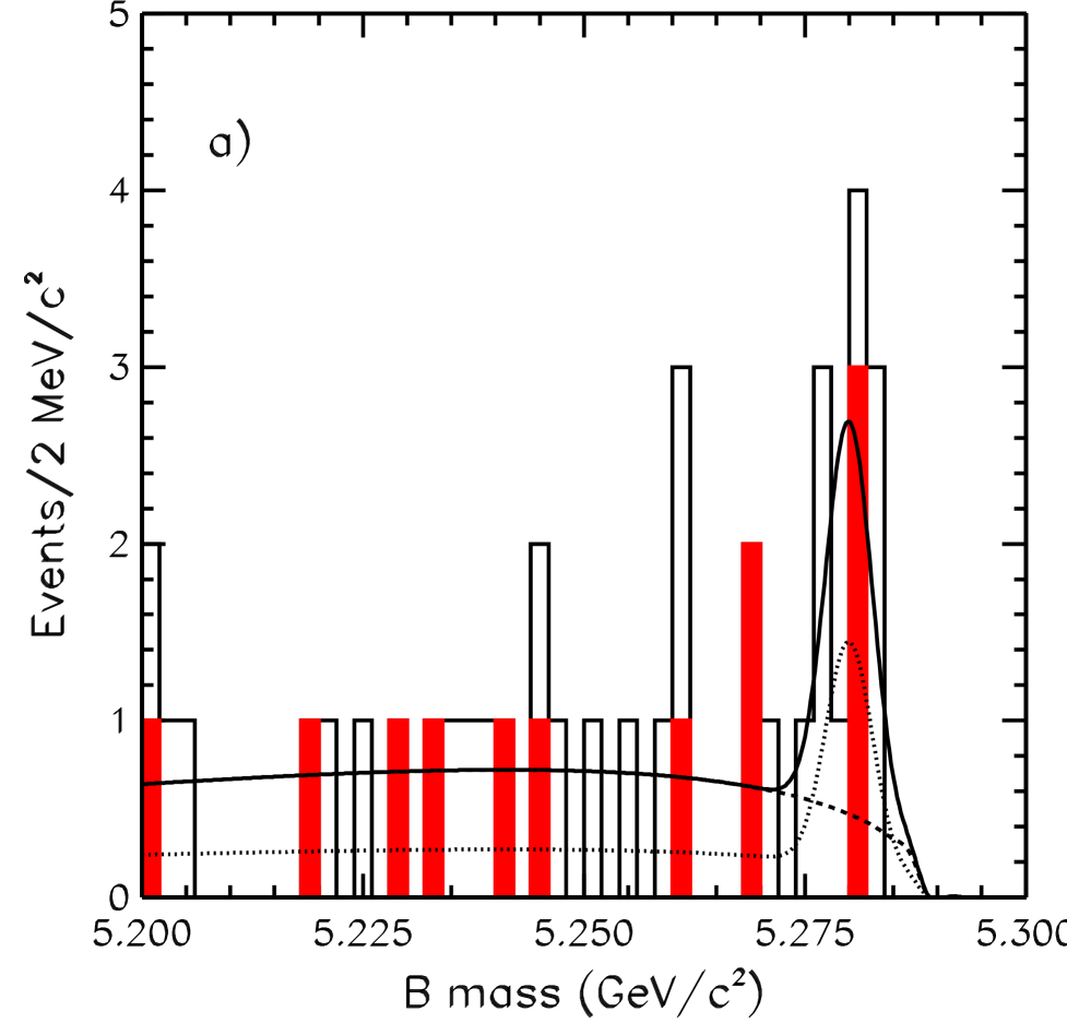
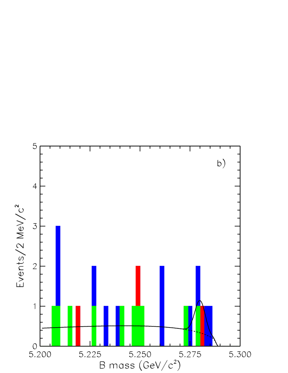
FIG. 8.: (a) Likelihood function contours for $B^{+}\rightarrow\omega h^{+}$; (b) $-2\ln{\mbox{$\cal L$}/\mbox{$\cal L$}_{\rm max}}$ for $B\rightarrow\phi K^{*}$.

FIG. 9.: Projection onto the variable $M$ for (a) $B^{+}\rightarrow\omega K^{+}$(shaded) and $B^{+}\rightarrow\omega\pi^{+}$(open) and (b) $B\rightarrow\phi K^{*}$: $B^{0}\rightarrow\phi K^{*0}$ (dark shading), $B^{+}\rightarrow\phi K^{*+}(K^{*+}\rightarrow K^{0}\pi^{+}$, medium shading), and $B^{+}\rightarrow\phi K^{*+}(K^{*+}\rightarrow K^{+}\pi^{0}$, light shading). The solid line shows the result of the likelihood fit, scaled to take into account the cuts applied to variables not shown. The dashed line shows the background component, and in (a) the dotted line shows the $B^{+}\rightarrow\omega K^{+}$ component of the fit only.

TABLE VI.: Combined results for $\omega$ and $\phi$ decay modes and expectations from theoretical models.

Decay mode	$\cal B$($10^{-5})$	Theory $\cal B$ ($10^{-5}$)	References
$B^{+}\rightarrow\omega K^{+}$	$1.5^{+0.7}_{-0.6}\pm 0.2$	$0.1-0.7$	[17, 20, 24, 26]
$B^{0}\rightarrow\omega K^{0}$	$<5.7$	$0.1-0.4$	[17, 20, 26]
$B^{+}\rightarrow\omega\pi^{+}$	$<2.3$	$0.1-0.7$	[17, 20, 24, 26]
$B^{+}\rightarrow\omega h^{+}$	$2.5^{+0.8}_{-0.7}\pm 0.3$	-	-
$B^{0}\rightarrow\omega\pi^{0}$	$<1.4$	$0.01-1.2$	[17, 20, 26]
$B^{0}\rightarrow\omega{\eta^{\prime}}$	$<6.0$	$0.3-1.7$	[17, 26]
$B^{0}\rightarrow\omega\eta$	$<1.2$	$0.1-0.5$	[17, 26]
$B^{+}\rightarrow\omega K^{*+}$	$<8.7$	$0.04-1.5$	[17, 20, 23]
$B^{0}\rightarrow\omega K^{*0}$	$<2.3$	$0.2-0.8$	[17, 20]
$B^{+}\rightarrow\omega\rho^{+}$	$<6.1$	$1.0-2.5$	[17, 20, 23]
$B^{0}\rightarrow\omega\rho^{0}$	$<1.1$	$0.04$	[17]
$B^{0}\rightarrow\omega\omega$	$<1.9$	$0.04-0.3$	[17, 20]
$B^{+}\rightarrow\phi K^{+}$	$<0.5$	$0.07-1.6$	[16, 17, 20, 21, 22, 24, 26]
$B^{0}\rightarrow\phi K^{0}$	$<3.1$	$0.07-1.3$	[16, 17, 20, 21, 22, 26]
$B^{+}\rightarrow\phi\pi^{+}$	$<0.5$	$<<0.1$	[19, 20, 21, 24, 26]
$B^{0}\rightarrow\phi\pi^{0}$	$<0.5$	$<<0.1$	[19, 20, 21, 26]
$B^{0}\rightarrow\phi{\eta^{\prime}}$	$<3.1$	$<<0.1$	[19, 26]
$B^{0}\rightarrow\phi\eta$	$<0.9$	$<<0.1$	[19, 20, 26]
$B^{+}\rightarrow\phi K^{*+}$	$<4.1$	$0.02-3.1$	[16, 17, 20, 22, 23]
$B^{0}\rightarrow\phi K^{*0}$	$<2.1$	$0.02-3.1$	[16, 17, 20, 22]
$B^{+}\rightarrow\phi\rho^{+}$	$<1.6$	$<<0.1$	[19, 20, 23]
$B^{0}\rightarrow\phi\rho^{0}$	$<1.3$	$<<0.1$	[19, 20]
$B^{0}\rightarrow\phi\omega$	$<2.1$	$<<0.1$	[19, 20]
$B^{0}\rightarrow\phi\phi$	$<1.2$	none

IV Evidence for the inclusive decay $B\rightarrow{\eta^{\prime}}X_{S}$ from CLEO

Evidence also has been found for the inclusive decay $B\rightarrow{\eta^{\prime}}X_{S}$. In this analysis the state $X_{S}$ is defined as a charged kaon accompanied by from zero to four pions, of which at most one can be a $\pi^{0}$. The momentum of ${\eta^{\prime}}$ mesons, reconstructed with the decay chain ${\eta^{\prime}}\rightarrow\eta\pi^{+}\pi^{-}$, $\eta\rightarrow{\gamma\gamma}$, is required to be in the range $2.0<p_{\eta^{\prime}}<2.7$ GeV/c in order to reduce background from $b\rightarrow c$ processes. The values of $\Delta{\rm E}$ and $M$, as defined above, are required to satisfy $|\mbox{$\Delta{\rm E}$}|<0.1$ GeV and $M>5.275$ GeV.

FIG. 10.: The ${\eta^{\prime}}$ mass distribution for (a) on-resonance and (b) off-resonance data.

FIG. 11.: Distribution of $X_{S}$ mass for data (points with error bars) and possible backgrounds: $B\rightarrow D{\eta^{\prime}}$ (solid histogram) and $B\rightarrow D^{*}{\eta^{\prime}}$ (dashed histogram). The normalization of the backgrounds is arbitrary.

The ${\eta^{\prime}}$ mass distribution is shown in Fig. 11; a clear signal of $39\pm 10$ events is seen for on-resonance data and none for the off-resonance sample. The signal, obtained by subtracting the off-resonance data in bins of $X_{S}$ mass, is plotted in Fig. 11. Note the four events corresponding to $B^{+}\rightarrow{\eta^{\prime}}K^{+}$ and the absence of events in the $K^{*}(892)$ mass region, both consistent with the exclusive results given above. Also shown in Fig. 11 are distributions for potential background modes such as $B\rightarrow D{\eta^{\prime}}$ and $B\rightarrow D^{*}{\eta^{\prime}}$. Though these also tend to have large $X_{S}$ mass, they are more peaked than the data. These and other studies suggest that the observed signal does not arise primarily from color-suppressed $b\rightarrow c$ decays, though it is difficult to rule this out completely without better models of such processes. The efficiency is calculated assuming that the signal arises solely from gluonic penguin decays, with an equal admixture of $X_{S}$ states from the kaon mass up to $K_{4}^{*}(2200)$. The efficiency of ($5.5\pm 0.3$)% leads to $\mbox{$\cal B$}(\mbox{$B\rightarrow{\eta^{\prime}}X_{S}$})=(6.2\pm 1.6\pm 1.3)\times 10^{-4}$ for $2.0<p_{\eta^{\prime}}<2.7$ GeV/c. The systematic error is dominated by the uncertainty in the $X_{S}$ modelling.

V Conclusion

CLEO has observed for the first time five charmless hadronic $B$ decay modes. The measured branching fractions range from (1–7)$\times 10^{-5}$. All of these modes involve $K$ mesons while none of the related modes involving pions have yet been observed. This suggests that penguin loop diagrams are playing a dominant role in these decays. These new results have sparked a considerable amount of theoretical activity during 1997. Fleischer and Mannel [27] claim that the fact that the ratio of the $K^{\pm}\pi^{\mp}$ and $K^{0}\pi^{\pm}$ modes is less than one (with large errors) may soon facilitate useful bounds on the CKM angle $\gamma$. Many recent papers point out that rescattering effects and electroweak penguins may complicate or invalidate this method.

The branching fraction for $B^{+}\rightarrow{\eta^{\prime}}K^{+}$, $(6.5^{+1.5}_{-1.4}\pm 0.9)\times 10^{-5}$, is several times larger than other charmless hadronic $B$ decays. This was unexpected, though it had been pointed out by Lipkin [28] that interference effects between the two penguin diagrams, Fig. 1e and 1f, enhance the ${\eta^{\prime}}K$ rate and suppress $\eta K^{+}$. The branching fractions and upper limits given in Table IV clearly exhibit this pattern. There have been a variety of recent effective-Hamiltonian calculations [29] which try to account for processes measured here, the large rate for $B\rightarrow{\eta^{\prime}}K$ in particular. They generally employ spectator and factorization [30] approximations, though the validity of the latter has been established only in $b\rightarrow c$ processes. These calculations have suggested enhancements from larger form factors [31, 32], smaller strange-quark mass [32], and variation of the effective number of colors [29, 33]. Others have suggested a contribution from the QCD gluon anomaly (Fig. 1h) or other flavor singlet processes in constructive interference with the penguins [34, 35, 36, 37, 38]. Given the experimental errors, most of these calculations can account for the data, though the models with additional singlet contributions appear to be needed unless the branching fraction for $B^{+}\rightarrow{\eta^{\prime}}K^{+}$ is reduced substantially when further data is obtained.

The theoretical situation with the $\omega$ and $\phi$ modes is also quite interesting. We also establish 90% CL lower limits on the branching fractions $B^{+}\rightarrow\omega K^{+}$ and $B^{+}\rightarrow\omega h^{+}$ of $8.4\times 10^{-6}$ and $1.6\times 10^{-5}$, respectively. Predictions for these rates tend to be smaller than the observed rate for most values of the color parameter $\xi$ [29, 33, 37]. Predictions for $B^{+}\rightarrow\phi K^{+}$ tend to be larger than the limited presented here; the combination of these upper and lower limits rules out all values of $\xi$ for these models at $>90$% CL, though additional variation of theoretical parameters could probably account for the data. A recent calculation [39], involving an enhanced contribution from charmed quarks in the penguin loop, also has difficulty accounting for a large rate in the $\omega K^{+}$ channel but predicts large branching fractions for final states such as $\omega K^{*}$ and $\phi K^{*}$.

There have also been many attempts to explain the even more surprising excess of ${\eta^{\prime}}$ inclusive events. Atwood and Soni [34] first suggested an enhancement in this process arising from the anomalous coupling of gluons with the ${\eta^{\prime}}$ meson, analogous to the exclusive diagram shown in Fig. 1h. Other authors [31, 32, 41, 42] have considered this process, though without a consensus whether the anomaly can account for the inclusive rate. Prospects are excellent for resolution of many of these issues during 1998 as new data become available.

REFERENCES

- [1] M. Kobayashi and T. Maskawa, Prog. Theor. Phys. 49, 652 (1973).
- [2] For an excellent recent review of the subject, see A. J. Buras and R. Fleischer, Report No. TUM-HEP-275-97 (1997) to appear in Heavy Flavours II, World Scientific (1997), eds. A.J. Buras and M. Linder.
- [3] N.G. Deshpande and X-G. He, Phys. Rev. Lett. 76, 360 (1996).
- [4] M. Gronau and J. L. Rosner, Phys. Rev. D 53, 2516 (1996); A. S. Dighe, Phys. Rev. D 54, 2067 (1996); M. Gronau and J. L. Rosner, Phys. Rev. Lett. 76, 1200 (1996).
- [5] CLEO Collaboration, M. Battle et al., Phys. Rev. Lett. 71, 3922 (1993).
- [6] CLEO Collaboration, D.M. Asner et al., Phys. Rev. D 53, 1039 (1996).
- [7] ALEPH Collaboration, D. Buskulic et al., Phys. Lett. B 384, 471 (1996).
- [8] DELPHI Collaboration, W. Adam et al., Z. Phys. C 72, 207 (1996).
- [9] CLEO Collaboration, Y. Kubota et al., Nucl Inst. Meth. 320, 66 (1992).
- [10] The and analyses use a similar (not “extended”) ML fit in which event fractions rather than the total numbers of events are used.
- [11] GEANT 3.15: R. Brun et al., CERN DD/EE/84-1.
- [12] H. Albrecht et al., Phys. Lett. B 241, 278 (1990); 254, 288 (1991).
- [13] CLEO Collaboration, R. Godang et al., Cornell preprint CLNS 97/1522 (1997, to be published in Phys. Rev. Lett.).
- [14] CLEO Collaboration, B. H. Behrens et al., Cornell preprint CLNS 97/1536 (1997, to be published in Phys. Rev. Lett.).
- [15] CLEO Collaboration, Cornell preprint CLNS 97/1537 (1997, submitted to Phys. Rev. Lett.).
- [16] N.G. Deshpande and J. Trampetic, Phys. Rev. D 41, 895 (1990).
- [17] L.-L. Chau et al., Phys. Rev. D 43, 2176 (1991). A private communication from H-Y. Cheng indicates that many of the and branching fraction predictions in this paper were too large. The revised prediction for is . See also reference REFERENCES.
- [18] H. Simma and D. Wyler, Phys. Lett. B 272, 395 (1991).
- [19] D. Du and Z. Xing, Phys. Lett. B 312, 199 (1993).
- [20] A. Deandrea et al., Phys. Lett. B 318, 549 (1993); A. Deandrea et al., Phys. Lett. B 320, 170 (1994).
- [21] R. Fleischer, Z. Phys. C 58, 483 (1993); Phys. Lett. B 321, 259 (1994).
- [22] A.J. Davies, T. Hayashi, M. Matsuda, and M. Tanimoto, Phys. Rev. D 49, 5882 (1994).
- [23] G. Kramer, W. F. Palmer, and H. Simma, Nucl. Phys. B428 429 (1994).
- [24] G. Kramer, W. F. Palmer, and H. Simma, Zeit. Phys. C 66 429 (1995).
- [25] G. Kramer and W. F. Palmer, Phys. Rev. D 52, 6411 (1995)
- [26] D. Du and L. Guo, Z. Phys. C 75, 9 (1997).
- [27] R. Fleischer and T. Mannel, Phys. Rev. D 57, 2752 (1998).
- [28] H. J. Lipkin, Phys. Lett. B 254, 247 (1991).
- [29] A. Ali and C. Greub, Phys. Rev. D 57, 2996 (1998), and references therein.
- [30] M. Bauer, B. Stech, and M. Wirbel, Z. Phys. C 43, 103 (1987).
- [31] A. Datta, X-G. He, and S. Pakvasa, Report No. UH-511-864-97, hep-ph/9707259 (1997).
- [32] A. Kagan and A. Petrov, Report No. UCHEP-27, hep-ph/9707354 (1997).
- [33] N. G. Deshpande, B. Dutta, and S. Oh, Report No. OITS-641, hep-ph/9710354 (1997); Report No. OITS-644, hep-ph/9712445 (1997).
- [34] D. Atwood and A. Soni, Phys. Lett. B 405,150 (1997).
- [35] D. London and A. Soni, Phys. Lett. B 407, 61 (1997); A. S. Dighe, M. Gronau, and J. L. Rosner, Phys. Rev. Lett. 79, 4333 (1997).
- [36] M. R. Ahmady, E. Kou, and A. Sugamoto, Report No. RIKEN-AF-NP-274, hep-ph/9710509 (1997); D. Du, C. S. Kim, and Y. Yang, Report No. BIHEP-TH/97-15, hep-ph/9711428 (1997).
- [37] H-Y. Cheng and B. Tseng, Phys. Lett. B 415, 263 (1997).
- [38] I. Halperin and A. Zhitnitsky, Phys. Rev. D 56, 7247 (1997).
- [39] M. Ciuchini et al., Report No. CERN-TH-97-188, hep-ph/9708222 (1997).
- [40] A. S. Dighe, M. Gronau and J. L. Rosner, Phys. Rev. D 57, 1783 (1998).
- [41] W-S. Hou and B. Tseng, Phys. Rev. Lett. 80, 434 (1998).
- [42] F. Yuan and K-T. Chao, Phys. Rev. D 56, R2495 (1997).