Budker INP 98-02
                                                                        hep-ex/9802003
Physics goals and parameters of photon colliders

Abstract

Linear colliders offer a unique possibility to study $\gamma\gamma$ and $\gamma$e interactions at the energies 0.1–2 TeV. This option is now included in design reports of NLC, JLC and TESLA/SBLC. This paper includes: status of photon colliders, new possibilities in study of Higgs boson, ways to achieve high luminosities.

1 Introduction

It is very likely that linear colliders with the c.m.s energies of 0.2–2 TeV will be built sometime, may be in about ten years from now [1]. Besides e⁺e^-collisions, linear colliders give an unique possibility to study $\gamma\gamma$ and $\gamma$e interactions at energies and luminosities comparable to those in e⁺e^- collisions [2]-[4].

The basic scheme of a photon collider is shown in fig. 2.

Figure 1: Scheme of $\gamma\gamma$; $\gamma$e collider.

Figure 2: Crab-crossing scheme

Two electron beams after the final focus system are traveling toward the interaction point (IP). At a distance of about 0.1–1 cm upstream from the IP, at the conversion point (C), the laser beam is focused and Compton backscattered by electrons, resulting in the high energy beam of photons. With reasonable laser parameters one can “convert” most of the electrons into high energy photons. The photon beam follows the original electron direction of motion with a small angular spread of the order $1/\gamma$, arriving at the IP tightly focused, where it collides with a similar opposing high energy photon beam or with an electron beam. The photon spot size at the IP may be almost equal to that of electrons at IP, and, therefore, the luminosity of $\gamma\gamma$, $\gamma$e collisions will be of the same order of magnitude as the “geometric” luminosity of the basic $ee$ beams. The detailed discussion of photon colliders can be found in refs [3]-[6]. and in the Berkeley Workshop Proceedings [7].

As of today, this option is included into the Conceptual Design Reports of NLC [8], TESLA–SBLC [9], and JLC [10] linear colliders. All these projects foresee the second interaction regions for $\gamma\gamma$, $\gamma$e collisions.

This paper covers three topics:

• physics at photon colliders, paticularly some important remarks on new possibilities to study the Higgs boson in $\gamma\gamma$ collisions;

• parameters of photon colliders in ‘Zero design’ projects of linear colliders;

• ways to achieve very high luminosities.

2 Physics

2.1 General remarks

The physics in high energy $\gamma\gamma$, $\gamma$e colliders is very rich. The total number of papers devoted to this subject exceeds one thousand. Recent reviews of physics at photon colliders can be found, for instance, in TESLA/SBLC Conceptual Design Report [9] (with many references therein) and in the J.Jikia’s talk at “Photon 97” [11]. In this paper, besides some general words on the physics in $\gamma\gamma$, $\gamma$e collisions, I would like to discuss some new important aspects of the Higgs study in $\gamma\gamma$ collisions.

For scientific (and political) motivation of building photon colliders the following short list of physics goals can be presented:

1. Some phenomena can be better studied at photon colliders than with pp or e⁺e^- collisions, for example, the measurement of the two-photon decay width of the Higgs boson. Due the loop diagrams, all massive (even ultra-heavy) charged particles contribute to this width if their mass is originated by the Higgs mechanism. Some Higgs decay modes and its mass can be measured at $\gamma\gamma$ colliders better than in e⁺e^- or pp collisions (see the next section).

2. Cross sections for production of charged scalar, lepton and top pairs in $\gamma\gamma$ collisions are larger than those in e⁺e^- collisions approximately by a factor of 5 (see fig.  3); for WW production, this factor is even larger, about 10–20.

3. In $\gamma$e collisions, charged supersymmetric particles with masses higher than in e⁺e^- collisions can be produced (a heavy charged particle plus a light neutral), $\gamma\gamma$ collisions also provide higher accessible masses for particles which are produced as a single resonance in $\gamma\gamma$ collisions (such as the Higgs).

These examples together with the fact that the luminosity in $\gamma\gamma$ collisions is potentially higher than that in e⁺e^- collisions (see sect. 4) are very strong arguments in favor of photon colliders.

Figure 3: Comparison of cross sections for charged pair production in e⁺e^- and $\gamma\gamma$ collisions. The cross section $\sigma=(\pi\alpha^{2}/M^{2})f(x)$, P=S (scalars), F (fermions), W (W-bosons); M is particle mass, $x=W_{p\bar{p}}^{2}/4M^{2}$. The functions $f(x)$ are shown.

A typical distribution of $\gamma\gamma$ or $\gamma$e  luminosity on the invariant mass has high energy peaks at the maximum masses with widths $\Delta W_{\mbox{$\gamma\gamma$}}/W_{\mbox{$\gamma\gamma$}}\approx 0.15$, $\Delta W_{\mbox{$\gamma$e}}/W_{\mbox{$\gamma$e}}\approx 0.05$[6, 9]. Below the high energy peak, there is usually a flat part of the luminosity distribution with 1–10 times larger total luminosity (depending on details of the collision scheme).

Statistics equal to that in e⁺e^- collisons, can be achieved in $\gamma\gamma$ collisions with much smaller (at least by a factor of five) luminosity. Of course, in any case data in $\gamma\gamma$ and e⁺e^- collisions are complimentary to each other because the coresponding diagrams are different).

2.2 Higgs in $\gamma\gamma$ collisions

Search and study of the Higgs boson, the key particle of the Standard model, is one of the primary goals of linear colliders. The LEP-2 will put the lower limit on its mass ot about 95 GeV. Indirectly, from radiative corrections, it follows that the Higgs mass (if the Standard Model is correct) is $140^{+150}_{-80}$ GeV [12]. The MSSM predicts a mass of the lightest neutral Higgs less of than 130 GeV. So, the mass of the Higgs most probably lies in the region of 100$<M_{H}<$300 GeV. Some parameters of the SM Higgs (total width, $\gamma\gamma$ width, and main branching ratios) are presented in fig. 4  [18, 21].

Higgs production in $\gamma\gamma$ collisions has been considered in many papers. Unfortunately, different authors have used their own definitions of the $\gamma\gamma$ luminosity which often led to underestimation of the expected number of events for a given integrated $\gamma\gamma$ luminosity. In the present paper, we will directly compare the Higgs production cross sections in $\gamma\gamma$ and e⁺e^- collisions. I would like also to pay attention to some additional possibilities for Higgs studies at photon colliders connected with a very sharp edge in the $\gamma\gamma$ luminosity spectra.

Figure 4: Some of the SM Higgs branching ratios as a function of its mass [18, 21]. On the left figure [18], the total width and the $\gamma\gamma$ width (thick lines) are also shown.

The total Higgs width at masses below 400 GeV is much smaller than the characteristic width of $\gamma\gamma$ luminosity spectra (FWHM $\sim 10-15\%$ ), therefore the production rate is proportional to $d\mbox{$L_{\gamma\gamma}$}/W_{\mbox{$\gamma\gamma$}}$:

$$\dot{N}_{\mbox{$\gamma\gamma$}\ \to H}=\mbox{$L_{\gamma\gamma}$}\times\frac{d\mbox{$L_{\gamma\gamma}$}M_{H}}{d\mbox{$W_{\gamma\gamma}$}\mbox{$L_{\gamma\gamma}$}}\frac{4\pi^{2}\Gamma_{\mbox{$\gamma\gamma$}}(1+\lambda_{1}\lambda_{2})}{M^{3}_{H}}\equiv\mbox{$L_{\gamma\gamma}$}\times\sigma^{eff}.$$ (1)

where $\lambda_{i}$ is the photon helicity. Below we assume that the Higgs search and study is done utilizing the high energy peak of the $\gamma\gamma$ luminosity energy spectrum.

The effective cross section for $(d\mbox{$L_{\gamma\gamma}$}/d\mbox{$W_{\gamma\gamma}$})(M_{H}/\mbox{$L_{\gamma\gamma}$})=7$ and $1+\lambda_{1}\lambda_{2}=2$ is presented in fig. 6. Note that here $L_{\gamma\gamma}$ is defined as the $\gamma\gamma$ luminosity at the high energy luminosity peak ($z=\mbox{$W_{\gamma\gamma}$}/2E_{e}>0.65$ for $x=4.8$), thus ignoring the lower energy part of the luminosity spectrum, which is much less valuable for experiment. This luminosity is approximately equal to $0.25k^{2}\mbox{$L_{ee}$}(geom)$. For comparison, in the same figure the cross sections of the Higgs production in e⁺e^- collisions is shown. We see that for $M_{H}=$ 100–250 GeV the effective cross section in $\gamma\gamma$ collisions is larger than that in e⁺e^- collisions by a factor of about 5–30. This interesting fact has never been emphasized.

Figure 5: Cross sections for the Standard model Higgs in $\gamma\gamma$ and e⁺e^- collisions.

Figure 6: Shape of the $\gamma\gamma$ luminosity spectrum near the high energy edge. Here $z=W_{\mbox{$\gamma\gamma$}}/2E_{0}.$

How do we study the Higgs in $\gamma\gamma$ collisions? One obvious way is searching for a peak in the invariant mass distribution measured by the detector. This is the only method utilizing the broad luminosity spectrum. The mass resolution in this method can be somewhat better than the width of the high energy luminosity peak.

Another method is the energy scanning where we can use some important features of the $\gamma\gamma$ luminosity distribution: quite narrow width of high energy peak and a very sharp edge of luminosity distribution which is much narrower than the width of the luminosity peak and the detector resolution, see fig. 6. For $x=4.8$ the differential luminosity ($dL/dz$) reaches half of its maximum at $\Delta z=z_{max}-z=0.8\%$ (at $\rho=b/\gamma a_{e}=1$). During the scanning, we will observe a sharp increase in the visible cross section when the maximum energy of the $\gamma\gamma$ collider reaches $M_{H}$ (if the Higgs is a very narrow resonance). Observation of a step at the same energy for different decay modes significantly increases confidence of results, especially for modes with small branchings or with difficulties in reconstruction. For example, detection of the $H\to\tau\tau$ decay is a difficult task due to undetected neutrinos. The most reliable way to see this channel is to observe a step in visible cross section for events with the following selection criteria: two collinear low-multiplicity jets with unbalanced transverse momentum and with the energy of one jet not far from the maximum photon energy.

The total number of events for 10 fb^-1 of integrated $\gamma\gamma$ luminosity (as it was defined above) for the case when the peak of the luminosity spectrum sits at the Higgs boson mass is 13000 (18000) for $M_{H}$ = 130 (150) GeV respectively (follows from cross section given in fig. 6). That is a lot! Due to energy scanning, the statistics will be somewhat smaller, about $N\approx 0.5N_{peak}$. The number of events for various decay modes (without any cuts) is given in table 1.

Table 1: The number of Higgs events in various decay modes (no cuts) for $M_{H}$= 130 and 150 GeV and 10 fb^-1 of integrated $\gamma\gamma$ luminosity.

Mode	$b\bar{b}$	WW∗	ZZ∗	$\tau\tau$	$c\bar{c}$	gg	$\gamma\gamma$	$\gamma$ Z
Br $M_{H}(130)$	0.52	0.29	0.037	0.055	0.025	0.063	0.0022	0.0019
events	3400	1900	240	350	160	410	15	12
Br $M_{H}(150)$	0.18	0.67	0.083	0.019	0.008	0.03	0.0014	0.002
events	1600	6000	750	171	74	260	13	22

The Higgs production at photon colliders and various backgrounds have been studied in many papers for various decay modes: $b\bar{b}\;$ [13]-[20]; ZZ [14, 15, 22]; WW [14, 15, 23, 24].

Below $M_{H}<150$ GeV, the SM Higgs decays mainly into $b\bar{b}$ pairs. The main backgrounds here are the QED processes $\mbox{$\gamma\gamma$}\ \to b\bar{b},\;c\bar{c}$, which can be suppressed using vertex detectors and polarized photon beams ($\sigma_{\gamma\gamma\to q\bar{q}}\propto 1-\lambda_{1}\lambda_{2}$, while $\sigma_{\gamma\gamma\to H}\propto 1+\lambda_{1}\lambda_{2}$). The remaining background is small.

For $M_{H}>190$ GeV, the Higgs can be observed in the best way in the ZZ decay mode. The main background here is the process $\gamma\gamma\to WW$, which can be suppressed by requiring that at least one of the Z’s be detected in $l^{+}l^{-}$ decay modes. In this channel, the SM Higgs can be observed in the range $M_{H}\sim$ 120 – 350 GeV. At higher masses, the Higgs signal will be much smaller than irreducible background $\gamma\gamma\to ZZ$ [22].

In the region $M_{H}>140$ GeV, the SM Higgs decays mainly into $WW$ (or $WW^{*}$) pairs. The main problem here is the background from $\gamma\gamma\to WW$ with large cross section. Fortunately, this background is very small for $M_{H}<2M_{W}$ [15, 23, 24], so that Higgs with $100<M_{H}<160$ GeV can be detected in this channel practically without backgrounds.

In the region $M_{H}>160$ GeV, the interference between the Higgs signal and the background becomes important [23, 24]. The cross section of $\mbox{$\gamma\gamma$}\ \to$ WW for various Higgs masses is shown in fig. 7 (the left figure is taken from ref.[23], the right one from ref.[24]) These cross sections correspond to monochromatic photon beams. In a real situation the photon beam energy spread and the detector resolution are much larger than the Higgs width, so that the resonance structures is much broader but nevertheless observable for not too large $M_{H}$. For $M_{H}>2M_{W}$, there are four additional constraints in the 4-jet decay mode: two come from the zero transverse momentum of the system, and two come from the jet-jet mass equal to $M_{W}$. Using of these constraints should improve the WW invariant mass resolution.

Much better sensitivity to narrow structures can be obtained utilizing the sharp edge of the $\gamma\gamma$ luminosity spectrum. Using all these methods, one can see the Higgs in $\mbox{$\gamma\gamma$}\ \to WW$ decay mode from $M_{H}\sim 100$ GeV up to $M_{H}\sim$ 200–250 GeV or even the higher.

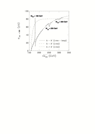
Figure 7: The $\gamma\gamma\to WW$ cross section for various Higgs masses, see comments in the text

Detection of the Higgs in $\tau\tau,cc,gg,\gamma\gamma,\gamma Z$ decays are also possible at photon colliders. In $\gamma\gamma$ and $\gamma Z$ modes, the background is rather small [25, 26]. Conclusions on perspectives of Higgs detection in these modes and required luminosities can be made only after a detail simulation.

Photon colliders also allow to measure the Higgs mass with a high precision. The very sharp edge of the luminosity spectrum and high statistics make it possible to obtain a much better accuracy than in e⁺e^- or pp collisions. In this measurement, it is important to remember that nonlinear effects in the conversion region can shift the maximum energy of Compton photons and change the shape of the luminosity spectrum [5, 6]. To reduce this effect, the parameter $\xi^{2}$ characterizing nonlinearity should be kept small enough. The shape of the luminosity spectrum near $z_{max}$ should be measured very precisely using the processes $\mbox{$\gamma\gamma$}\ \to\mu\mu\;(\mbox{e${}^{+}$e${}^{-}$})$.

As we have seen, the Higgs can be very successfully studied in $\gamma\gamma$ collisions for $M_{H}$ = 100–350 GeV, may be even better than in e⁺e^- collisions.

3 Luminosity

3.1 Current projects

Due to the absence of beamstrahlung, beams in $\gamma\gamma$ collisions can have much smaller horizontal beam size than in e⁺e^- collisions, thus the beta functions at the interaction point can be made as small as possible (some restrictions are imposed by the Oide effect connected with chromatic aberrations due to synchrotron radiation in the final quads). However, even after optimization of the final focusing system the attainable $\gamma\gamma$ luminosity in curent LC projects is determined by the attainable “geometric” ee–luminosity.

The results of simulations for different projects are the following. For the “nominal” beam parameters (the same as in e⁺e^- collisions) and the optimum final focus system the luminosity $\mbox{$L_{\gamma\gamma}$}(z>0.65)\sim(0.8/1.2/0.7)\times 10^{33}$ cm^-2s^-1 for NLC/TESLA/SBLC, or by about factor 5 smaller than e⁺e^- luminosity.

Obviously, this is not a fundamental limit. Below we will discuss what the limit really is and how to approach it.

3.2 Ultimate luminosity

The only collision effect restricting $\gamma\gamma$ luminosity at photon colliders is the coherent pair creation which leads to the conversion of a high energy photon into e⁺e^- pair in the field of the opposing electron beam [27, 5, 6]. There are three ways to avoid this effect: a) use flat beams; b) deflect the electron beam after conversion at a sufficiently large distance from the IP; c) under certain conditions (low beam energy, long bunches) the beam field at the IP is below the critical one due to the repulsion of electron beams [28]. The problem of ultimate luminosities for different beam parameters and energies was analyzed recently in ref.[29] analytically and by simulation. The resume is following.

The maximum luminosity is attained when the conversion point is situated as close as possible to the IP, at $b\approx 3\sigma_{z}+0.04E[\mbox{TeV}]$ cm (here the second term is equal to the minimum length of the conversion region). In this case, the vertical radius of the photon beam at the IP is also minimal: $a_{\gamma}\sim b/\gamma$ (assuming that the vertical size of the electron beam is even smaller). The optimal horizontal beam size ($\sigma_{x}$) depends on the beam energy, the number of particles in a bunch and the bunch length. The dependence of the $\gamma\gamma$ luminosity on $\sigma_{x}$ for various energies and numbers of particles per bunch is shown in fig. 8. The bunch length is fixed at 0.2 mm. The collision rate is calculated from the total beam power, which is equal to 15E[TeV] MW (close to that in current projects). From the fig. 8 we see that at low energies and small numbers of particles, the luminosity curves follow their natural behavior $L\propto 1/\sigma_{x}$, while at high energies and large numbers of particles per bunch the curves make a zigzag which is explained by $\gamma\to$ e⁺e^- conversion in the field of the opposing beam.

Figure 8: Dependence of the $\gamma\gamma$ luminosity on the horizontal beam size for $\sigma_{z}=0.2$ mm, see comments in the text.

What is so remarkable about these results? First of all, the maximum attainable luminosities are huge, above $10^{35}$ cm^-2s^-1. At low energies, there is no coherent pair creation, even for a very small $\sigma_{x}$’s, when the field in the beam is much higher than the critical field $B_{cr}=\alpha e/\gamma r^{2}_{e}$. This is explained by the fact that during the collision the beams are repulsing each other so that the field on the beam axis (which affects high energy photons) is below the critical field. It means that the $\gamma\gamma$ luminosity is simply proportional to the geometric electron-electron luminosity (approximately $\mbox{$L_{\gamma\gamma}$}(z>0.65)\sim 0.1L_{ee}$) for $\sigma_{x},\sigma_{y}<b/\gamma\sim 3\sigma_{z}/\gamma+0.2$ nm. For energies 2E$<$ 2 TeV, which are in reach of the next generation of linear colliders, the luminosity limit is much higher than it is usually required and much higher than in e⁺e^- collisions (especially at low energies).

One of the main problems in obtaining such high $\gamma\gamma$ luminosity is generation of electron beams with small emittances in both horizontal and vertical directions. In the following sections we will discuss various approaches to solving this problems.

3.3 Ways to higher luminosities

There are several possibilities for increasing luminosity.

1) Reduction of the horizontal emittance by optimizing the damping rings. For example, at the TESLA, a decrease of $\epsilon_{nx}$ by a factor of 3.5 leads to an increase in $L_{\gamma\gamma}$ up to $3\times 10^{33}$ cm^-2s^-1. However, it seems that this way is quite difficult.

2) One can use low emittance RF-photoguns instead of damping rings. Unfortunately, even with the best photoguns the luminosity will be somewhat lower than that with damping rings. However, there is one possible solution. The normalized emittance in photoguns is approximately proportional to the number of particles in the electron bunch. It seems possible to merge (using some difference in energies) many ($N_{g}\sim 5-10$) low current beams with low emittances to one high current beam with the same transverse emittance. This gives us a gain in luminosity more than by a factor of $N_{g}$ in comparison with a single photogun (“more” because the lower emittance allows smaller beta functions due to the Oide effect). Estimations show that with ten photoguns, one can achieve $L_{\gamma\gamma}$ $\sim L_{\mbox{e${}^{+}$e${}^{-}$}}$ in all considered projects. There is only one “small” problem: such RF-guns with polarized electrons do not exist yet, though there are no visible fundamental problems [31]. Also there is the “thermal” limit on emittance in photoguns, which puts some restrictions on this method. In the AsGa photoguns with polarized electrons, this limit should be much smaller than for metal photocathodes [31].

3) If one has flat electron beams ($\epsilon_{nx}$$>>$ $\epsilon_{ny}$) from some injector (a damping ring or, better, an RF-gun), then it is possible, in principle, to make exchange of the horizonlal and longitudinal emittances using an off-axis RF cavity (some head-tail kick arizing here can be removed by additional RF cavities rotated by 90⁰. This method was never tested or even discussed. I do not know why. This method is especially promising for beams from RF-guns, where very small energy spread allows both horizontal and longitudinal beam compression. This method as well as the previous one should be studied more carefully.

4) For a considerable step up in luminosity, beams with much lower emittances are required. That needs development of new approaches, such as laser cooling [30] (see next subsection). Potentially, this method allows to attain a geometric luminosity by two orders higher than that achievable by other known methods.

3.4 Laser cooling

Recently [30], a new method of beam production with small emittance was considered — laser cooling of electron beams — which allows, in principle, to reach $\mbox{$L_{\gamma\gamma}$}\geq 10^{35}$ cm^-2s^-1.

The idea of laser cooling of electron beams is very simple. During a collision with optical laser photons (in the case of strong fields it is more appropriate to consider the interaction of an electron with an electromagnetic wave) the transverse distribution of electrons ($\sigma_{i}$) remains almost the same. Also, the angular spread ($\sigma_{i}^{\prime}$) is almost constant, because electrons loss momenta almost along their trajectory (photons follow the initial electron trajectory with a small additional spread). So, the emittance $\mbox{$\epsilon_{i}$}=\mbox{$\sigma_{i}$}\mbox{$\sigma_{i}^{\prime}$}$ remains almost unchanged. At the same time, the electron energy decreases from $E_{0}$ down to $E$. This means that the transverse normalized emittances have decreased: $\mbox{$\epsilon_{n}$}=\gamma\mbox{$\epsilon$}=\mbox{$\epsilon_{n}$}_{0}(E/E_{0})$. One can reaccelerate the electrons up to the initial energy and repeat the procedure. Then after N stages of cooling $\mbox{$\epsilon_{n}$}/\mbox{$\epsilon_{n}$}_{0}=(E/E_{0})^{N}$ (if $\epsilon_{n}$ is far from its limit).

Some possible set of parameters for laser cooling is: $E_{0}=4.5$ GeV, $l_{e}=0.2$ mm, $\lambda=0.5$ $\mu$m, flash energy $A\sim 10$ J. The final electron bunch will have an energy of 0.45 GeV with an energy spread $\sigma_{E}/E\sim 13\%$, the normalized emittances $\epsilon_{nx}$,$\epsilon_{ny}$ are reduced by a factor of 10. A two-stage system with the same parameters reduces the emittances by a factor of 100. The limit on the final emittance is $\mbox{$\epsilon_{nx}$}\ \sim\mbox{$\epsilon_{ny}$}\ \sim 2\times 10^{-9}\;$ m rad at $\beta_{i}=1\;\mbox{mm}$. For comparison, in the TESLA (NLC) project the damping rings have $\mbox{$\epsilon_{nx}$}\ =14(3)\times 10^{-6}\;$ m rad, $\mbox{$\epsilon_{ny}$}\ =25(3)\times 10^{-8}\;$ m rad.

This method requires a laser system even more powerful than that for e $\to\gamma$ conversion. However, all the requirements are reasonable, taking into account the fast progress of laser technique and time plans of linear colliders. Multiple use of the laser bunch (some optical resonator) can considerably reduce the required average laser power. This method can be tested already now at a low repeatition rate.

4 Acknowledgements

I would like to thank Clem Heusch for a nice Workshop, which was one of the important steps towards e⁺e^-, ee, $\gamma$e, $\gamma\gamma$ colliders.

References

- [1] G. Loew et al., Int. Linear Collider Tech. Rev. Com. Rep., SLAC-Rep-471(1996).
- [2] I.Ginzburg, G.Kotkin, V.Serbo, V.Telnov, Pizma ZhETF, 34 (1981) 514; JETP Lett.34 (1982) 491.
- [3] I.Ginzburg, G.Kotkin, V.Serbo, V.Telnov, Nucl. Instr. and Meth. 205 (1983) 47.
- [4] I.Ginzburg, G.Kotkin, S.Panfil, V.Serbo, V.Telnov, Nucl. Instr. and Meth. 219 (1984) 5.
- [5] V.Telnov, Nucl. Instr. and Meth.A 294 (1990) 72.
- [6] V.Telnov, Nucl. Instr. and Meth.A 355 (1995) 3.
- [7] Proc.of Workshop on Colliders, Berkeley CA, USA, 1994, Nucl. Instr. and Meth. A 355 (1995) 1–194.
- [8] Zeroth-Order Design Report for the Next Linear Collider LBNL-PUB-5424, SLAC Report 474, May 1996.
- [9] Conceptual Design of a 500 GeV Electron Positron Linear Collider with Integrated X-Ray Laser Facility DESY 79-048, ECFA-97-182, e-print: hep-ex/9707017.
- [10] JLC Design Study, KEK-REPORT-97-1, April 1997.
- [11] J.Jikia, Proc. the Intern. Conference “Photon 97”, Egmond ann Zee, The Netherland, May 10–15, 1997, Freiburg-THEP 97/11, e-print: hep-ph/9706508.
- [12] A.Blondel, Proc. of the 28th Int.Conf.on High Energy Physics, Warsaw, Poland, July 1996, World Scientific, p.205.
- [13] T. Barklow, Proc. of the 1990 DPF Summer Study on High-Energy Physics: “Research Directions for the Decade”, Snowmass, CO, June 25, 1990, p. 440.
- [14] D.L. Borden, D.A. Bauer, D.O. Caldwell, Phys. Rev. D48 (1993) 4018.
- [15] J.F. Gunion and H.E. Haber, Phys. Rev. D48 (1993) 5109.
- [16] G. Jikia, A. Tkabladze, Phys. Rev D54 (1996) 2030; hep-ph/9601384.
- [17] D. L. Borden, V. A. Khoze, W. J. Stirling, and J. Ohnemus, Phys. Rev. D50 (1994) 4499.
- [18] M. Baillargeon, G. Belanger, and F. Boudjema, Proc. of the “Two-Photon Physics from to LEP200 and Beyond”, 2-4 February 1994, Paris, ENSLAPP-A-473-94, hep-ph/9405359.
- [19] M. Baillargeon, G. Belanger and F. Boudjema, Phys. Rev. D51 (1995) 4712.
- [20] T.Ohgaki and T.Takahashi, Phys. Rev. D56 (1997) 1723, hep-ph/9703301.
- [21] A.Djouadi, J.Kalinowski, M.Spira, prep DESY-97-079, hep-ph/9704448.
- [22] G. Jikia, Phys. Lett. B298 (1993) 224; Nucl. Phys. B405 (1993) 24.
- [23] D.A.Morris, T.N.Truong and D.Zappala, Phys.Lett., B 323 (1994) 421.
- [24] I.Ginzburg, I.Ivanov, Phys.Lett., B 408 (1997) 325.
- [25] G. Jikia, A. Tkabladze, Phys. Lett. B323 (1994) 453.
- [26] G. Jikia, A. Tkabladze, Phys. Lett. B332 (1994) 441.
- [27] P.Chen,V.Telnov, Phys.Rev.Letters, 63 (1989) 1796.
- [28] V.Telnov, Proc. of Workshop “Photon 95”, Sheffield, UK, April 1995, p.369.
- [29] V.Telnov, Proc. of ITP Workshop “Future High energy colliders” Santa Barbara, USA, October 21-25, 1996, AIP conf. proc. 397, Budker INP 97-47, e-print: physics/9706003.
- [30] V.Telnov, Proc. of ITP Workshop “New modes of particle acceleration techniques and sources” Santa Barbara, USA, August 1996, AIP conf. proc. 396, NSF-ITP-96-142, SLAC-PUB 7337, Phys.Rev.Lett., 78 (1997) 4757, hep-ex/9610008.
- [31] J.Clendenin, private communication.