EUROPEAN LABORATORY FOR PARTICLE PHYSICS

CERN-PPE/97-152

4 December 1997

Measurement of the one-prong hadronic tau branching ratios at LEP

The OPAL Collaboration

Abstract

The branching ratios of the $\tau^{-}\rightarrow h^{-}\,\nu_{\tau}$, $\tau^{-}\rightarrow h^{-}\,\pi^{0}\nu_{\tau}$ and $\tau^{-}\rightarrow h^{-}\,\geq 2\pi^{0}\nu_{\tau}$ decays have been measured using the 1991–1995 data recorded with the OPAL detector at LEP. These branching ratios are measured simultaneously using three selection criteria and are found to be

BR($\tau^{-}\rightarrow h^{-}\,\nu_{\tau}$) = $(11.98\pm 0.13\pm 0.16)\,\%$ BR($\tau^{-}\rightarrow h^{-}\,\pi^{0}\nu_{\tau}$) = $(25.89\pm 0.17\pm 0.29)\,\%$ BR($\tau^{-}\rightarrow h^{-}\,\geq 2\pi^{0}\nu_{\tau}$) = $(9.91\pm 0.31\pm 0.27)\,\%$

where the first error is statistical and the second is systematic.

(To be submitted to Zeitschrift für Physik C)

The OPAL Collaboration

K. Ackerstaff⁸, G. Alexander²³, J. Allison¹⁶, N. Altekamp⁵, K.J. Anderson⁹, S. Anderson¹², S. Arcelli², S. Asai²⁴, S.F. Ashby¹, D. Axen²⁹, G. Azuelos^18,a, A.H. Ball¹⁷, E. Barberio⁸, R.J. Barlow¹⁶, R. Bartoldus³, J.R. Batley⁵, S. Baumann³, J. Bechtluft¹⁴, C. Beeston¹⁶, T. Behnke⁸, A.N. Bell¹, K.W. Bell²⁰, G. Bella²³, S. Bentvelsen⁸, S. Bethke¹⁴, S. Betts¹⁵, O. Biebel¹⁴, A. Biguzzi⁵, S.D. Bird¹⁶, V. Blobel²⁷, I.J. Bloodworth¹, J.E. Bloomer¹, M. Bobinski¹⁰, P. Bock¹¹, D. Bonacorsi², M. Boutemeur³⁴, S. Braibant⁸, L. Brigliadori², R.M. Brown²⁰, H.J. Burckhart⁸, C. Burgard⁸, R. Bürgin¹⁰, P. Capiluppi², R.K. Carnegie⁶, A.A. Carter¹³, J.R. Carter⁵, C.Y. Chang¹⁷, D.G. Charlton^1,b, D. Chrisman⁴, P.E.L. Clarke¹⁵, I. Cohen²³, J.E. Conboy¹⁵, O.C. Cooke⁸, C. Couyoumtzelis¹³, R.L. Coxe⁹, M. Cuffiani², S. Dado²², C. Dallapiccola¹⁷, G.M. Dallavalle², R. Davis³⁰, S. De Jong¹², L.A. del Pozo⁴, K. Desch³, B. Dienes^33,d, M.S. Dixit⁷, M. Doucet¹⁸, E. Duchovni²⁶, G. Duckeck³⁴, I.P. Duerdoth¹⁶, D. Eatough¹⁶, J.E.G. Edwards¹⁶, P.G. Estabrooks⁶, H.G. Evans⁹, M. Evans¹³, F. Fabbri², A. Fanfani², M. Fanti², A.A. Faust³⁰, L. Feld⁸, F. Fiedler²⁷, M. Fierro², H.M. Fischer³, I. Fleck⁸, R. Folman²⁶, D.G. Fong¹⁷, M. Foucher¹⁷, A. Fürtjes⁸, D.I. Futyan¹⁶, P. Gagnon⁷, J.W. Gary⁴, J. Gascon¹⁸, S.M. Gascon-Shotkin¹⁷, N.I. Geddes²⁰, C. Geich-Gimbel³, T. Geralis²⁰, G. Giacomelli², P. Giacomelli⁴, R. Giacomelli², V. Gibson⁵, W.R. Gibson¹³, D.M. Gingrich^30,a, D. Glenzinski⁹, J. Goldberg²², M.J. Goodrick⁵, W. Gorn⁴, C. Grandi², E. Gross²⁶, J. Grunhaus²³, M. Gruwé⁸, C. Hajdu³², G.G. Hanson¹², M. Hansroul⁸, M. Hapke¹³, C.K. Hargrove⁷, P.A. Hart⁹, C. Hartmann³, M. Hauschild⁸, C.M. Hawkes⁵, R. Hawkings²⁷, R.J. Hemingway⁶, M. Herndon¹⁷, G. Herten¹⁰, R.D. Heuer⁸, M.D. Hildreth⁸, J.C. Hill⁵, S.J. Hillier¹, P.R. Hobson²⁵, A. Hocker⁹, R.J. Homer¹, A.K. Honma^28,a, D. Horváth^32,c, K.R. Hossain³⁰, R. Howard²⁹, P. Hüntemeyer²⁷, D.E. Hutchcroft⁵, P. Igo-Kemenes¹¹, D.C. Imrie²⁵, M.R. Ingram¹⁶, K. Ishii²⁴, A. Jawahery¹⁷, P.W. Jeffreys²⁰, H. Jeremie¹⁸, M. Jimack¹, A. Joly¹⁸, C.R. Jones⁵, G. Jones¹⁶, M. Jones⁶, U. Jost¹¹, P. Jovanovic¹, T.R. Junk⁸, J. Kanzaki²⁴, D. Karlen⁶, V. Kartvelishvili¹⁶, K. Kawagoe²⁴, T. Kawamoto²⁴, P.I. Kayal³⁰, R.K. Keeler²⁸, R.G. Kellogg¹⁷, B.W. Kennedy²⁰, J. Kirk²⁹, A. Klier²⁶, S. Kluth⁸, T. Kobayashi²⁴, M. Kobel¹⁰, D.S. Koetke⁶, T.P. Kokott³, M. Kolrep¹⁰, S. Komamiya²⁴, T. Kress¹¹, P. Krieger⁶, J. von Krogh¹¹, P. Kyberd¹³, G.D. Lafferty¹⁶, R. Lahmann¹⁷, W.P. Lai¹⁹, D. Lanske¹⁴, J. Lauber¹⁵, S.R. Lautenschlager³¹, J.G. Layter⁴, D. Lazic²², A.M. Lee³¹, E. Lefebvre¹⁸, D. Lellouch²⁶, J. Letts¹², L. Levinson²⁶, S.L. Lloyd¹³, F.K. Loebinger¹⁶, G.D. Long²⁸, M.J. Losty⁷, J. Ludwig¹⁰, D. Lui¹², A. Macchiolo², A. Macpherson³⁰, M. Mannelli⁸, S. Marcellini², C. Markopoulos¹³, C. Markus³, A.J. Martin¹³, J.P. Martin¹⁸, G. Martinez¹⁷, T. Mashimo²⁴, P. Mättig²⁶, W.J. McDonald³⁰, J. McKenna²⁹, E.A. Mckigney¹⁵, T.J. McMahon¹, R.A. McPherson⁸, F. Meijers⁸, S. Menke³, F.S. Merritt⁹, H. Mes⁷, J. Meyer²⁷, A. Michelini², G. Mikenberg²⁶, D.J. Miller¹⁵, A. Mincer^22,e, R. Mir²⁶, W. Mohr¹⁰, A. Montanari², T. Mori²⁴, U. Müller³, S. Mihara²⁴, K. Nagai²⁶, I. Nakamura²⁴, H.A. Neal⁸, B. Nellen³, R. Nisius⁸, S.W. O’Neale¹, F.G. Oakham⁷, F. Odorici², H.O. Ogren¹², A. Oh²⁷, N.J. Oldershaw¹⁶, M.J. Oreglia⁹, S. Orito²⁴, J. Pálinkás^33,d, G. Pásztor³², J.R. Pater¹⁶, G.N. Patrick²⁰, J. Patt¹⁰, R. Perez-Ochoa⁸, S. Petzold²⁷, P. Pfeifenschneider¹⁴, J.E. Pilcher⁹, J. Pinfold³⁰, D.E. Plane⁸, P. Poffenberger²⁸, B. Poli², A. Posthaus³, C. Rembser⁸, S. Robertson²⁸, S.A. Robins²², N. Rodning³⁰, J.M. Roney²⁸, A. Rooke¹⁵, A.M. Rossi², P. Routenburg³⁰, Y. Rozen²², K. Runge¹⁰, O. Runolfsson⁸, U. Ruppel¹⁴, D.R. Rust¹², R. Rylko²⁵, K. Sachs¹⁰, T. Saeki²⁴, W.M. Sang²⁵, E.K.G. Sarkisyan²³, C. Sbarra²⁹, A.D. Schaile³⁴, O. Schaile³⁴, F. Scharf³, P. Scharff-Hansen⁸, J. Schieck¹¹, P. Schleper¹¹, B. Schmitt⁸, S. Schmitt¹¹, A. Schöning⁸, M. Schröder⁸, H.C. Schultz-Coulon¹⁰, M. Schumacher³, C. Schwick⁸, W.G. Scott²⁰, T.G. Shears¹⁶, B.C. Shen⁴, C.H. Shepherd-Themistocleous⁸, P. Sherwood¹⁵, G.P. Siroli², A. Sittler²⁷, A. Skillman¹⁵, A. Skuja¹⁷, A.M. Smith⁸, G.A. Snow¹⁷, R. Sobie²⁸, S. Söldner-Rembold¹⁰, R.W. Springer³⁰, M. Sproston²⁰, K. Stephens¹⁶, J. Steuerer²⁷, B. Stockhausen³, K. Stoll¹⁰, D. Strom¹⁹, R. Ströhmer³⁴, P. Szymanski²⁰, R. Tafirout¹⁸, S.D. Talbot¹, S. Tanaka²⁴, P. Taras¹⁸, S. Tarem²², R. Teuscher⁸, M. Thiergen¹⁰, M.A. Thomson⁸, E. von Törne³, E. Torrence⁸, S. Towers⁶, I. Trigger¹⁸, Z. Trócsányi³³, E. Tsur²³, A.S. Turcot⁹, M.F. Turner-Watson⁸, P. Utzat¹¹, R. Van Kooten¹², M. Verzocchi¹⁰, P. Vikas¹⁸, E.H. Vokurka¹⁶, H. Voss³, F. Wäckerle¹⁰, A. Wagner²⁷, C.P. Ward⁵, D.R. Ward⁵, P.M. Watkins¹, A.T. Watson¹, N.K. Watson¹, P.S. Wells⁸, N. Wermes³, J.S. White²⁸, B. Wilkens¹⁰, G.W. Wilson²⁷, J.A. Wilson¹, T.R. Wyatt¹⁶, S. Yamashita²⁴, G. Yekutieli²⁶, V. Zacek¹⁸, D. Zer-Zion⁸

¹School of Physics and Astronomy, University of Birmingham, Birmingham B15 2TT, UK
²Dipartimento di Fisica dell’ Università di Bologna and INFN, I-40126 Bologna, Italy
³Physikalisches Institut, Universität Bonn, D-53115 Bonn, Germany
⁴Department of Physics, University of California, Riverside CA 92521, USA
⁵Cavendish Laboratory, Cambridge CB3 0HE, UK
⁶ Ottawa-Carleton Institute for Physics, Department of Physics, Carleton University, Ottawa, Ontario K1S 5B6, Canada
⁷Centre for Research in Particle Physics, Carleton University, Ottawa, Ontario K1S 5B6, Canada
⁸CERN, European Organisation for Particle Physics, CH-1211 Geneva 23, Switzerland
⁹Enrico Fermi Institute and Department of Physics, University of Chicago, Chicago IL 60637, USA
¹⁰Fakultät für Physik, Albert Ludwigs Universität, D-79104 Freiburg, Germany
¹¹Physikalisches Institut, Universität Heidelberg, D-69120 Heidelberg, Germany
¹²Indiana University, Department of Physics, Swain Hall West 117, Bloomington IN 47405, USA
¹³Queen Mary and Westfield College, University of London, London E1 4NS, UK
¹⁴Technische Hochschule Aachen, III Physikalisches Institut, Sommerfeldstrasse 26-28, D-52056 Aachen, Germany
¹⁵University College London, London WC1E 6BT, UK
¹⁶Department of Physics, Schuster Laboratory, The University, Manchester M13 9PL, UK
¹⁷Department of Physics, University of Maryland, College Park, MD 20742, USA
¹⁸Laboratoire de Physique Nucléaire, Université de Montréal, Montréal, Quebec H3C 3J7, Canada
¹⁹University of Oregon, Department of Physics, Eugene OR 97403, USA
²⁰Rutherford Appleton Laboratory, Chilton, Didcot, Oxfordshire OX11 0QX, UK
²²Department of Physics, Technion-Israel Institute of Technology, Haifa 32000, Israel
²³Department of Physics and Astronomy, Tel Aviv University, Tel Aviv 69978, Israel
²⁴International Centre for Elementary Particle Physics and Department of Physics, University of Tokyo, Tokyo 113, and Kobe University, Kobe 657, Japan
²⁵Brunel University, Uxbridge, Middlesex UB8 3PH, UK
²⁶Particle Physics Department, Weizmann Institute of Science, Rehovot 76100, Israel
²⁷Universität Hamburg/DESY, II Institut für Experimental Physik, Notkestrasse 85, D-22607 Hamburg, Germany
²⁸University of Victoria, Department of Physics, P O Box 3055, Victoria BC V8W 3P6, Canada
²⁹University of British Columbia, Department of Physics, Vancouver BC V6T 1Z1, Canada
³⁰University of Alberta, Department of Physics, Edmonton AB T6G 2J1, Canada
³¹Duke University, Dept of Physics, Durham, NC 27708-0305, USA
³²Research Institute for Particle and Nuclear Physics, H-1525 Budapest, P O Box 49, Hungary
³³Institute of Nuclear Research, H-4001 Debrecen, P O Box 51, Hungary
³⁴Ludwigs-Maximilians-Universität München, Sektion Physik, Am Coulombwall 1, D-85748 Garching, Germany

^a and at TRIUMF, Vancouver, Canada V6T 2A3
^b and Royal Society University Research Fellow
^c and Institute of Nuclear Research, Debrecen, Hungary
^d and Department of Experimental Physics, Lajos Kossuth University, Debrecen, Hungary
^e and Department of Physics, New York University, NY 1003, USA

1 Introduction

Precise tests of the Standard Model can be made using $\tau$ leptons [1]. Measurements of the $\tau$ allow the study of the structure of the weak currents and the universality of the couplings of the charged leptons to the gauge bosons, and can be used to search for evidence of new physics. Further, the $\tau$ is the only lepton to decay into hadrons, allowing the study of the strong interaction. For many of these studies an accurate knowledge of the properties of the $\tau$ is essential. In this paper we report on a measurement of the branching ratios of the $\tau^{-}\rightarrow h^{-}\,\nu_{\tau}$, $\tau^{-}\rightarrow h^{-}\,\pi^{0}\nu_{\tau}$ and $\tau^{-}\rightarrow h^{-}\,\geq 2\pi^{0}\nu_{\tau}$ decays using the 1991–1995 data recorded with the OPAL detector at LEP.

The measurement of the one-prong hadronic branching ratios is made by selecting a sample of tau decays with one track (one-prong) and then counting the number of $\pi^{0}$’s in each decay. The one-prong decays were subdivided into samples with $0$, $1$ or $\geq 2$ $\pi^{0}$’s from which the branching ratios for the three signal channels were determined. In Table 1 we list the $\tau$ decays that are included in each signal channel. We use the PDG definitions for these signal channels [2]. Note that not all modes were included in the Monte Carlo simulation. No attempt to separate charged pions and kaons was made in this measurement. The limited granularity of the OPAL electromagnetic calorimeter made it impossible to resolve unambiguously the decays with two $\pi^{0}$’s from those with three or more $\pi^{0}$’s with the $\pi^{0}$ identification algorithm used in this work, hence only a measurement of the $\geq 2\pi^{0}$ branching ratio is presented.

Selection	Decay mode	Weight	Comment
$\tau^{-}\rightarrow h^{-}\,\nu_{\tau}$	$\tau^{-}\rightarrow\pi^{-}\,\nu_{\tau}$
	$\tau^{-}\rightarrow{\rm K^{-}}\,\nu_{\tau}$
$\tau^{-}\rightarrow h^{-}\,\pi^{0}\nu_{\tau}$	$\tau^{-}\rightarrow\pi^{-}\,\pi^{0}\,\nu_{\tau}$
	$\tau^{-}\rightarrow{\rm K^{-}}\,\pi^{0}\,\nu_{\tau}$
$\tau^{-}\rightarrow h^{-}\,\geq 2\pi^{0}\nu_{\tau}$	$\tau^{-}\rightarrow\pi^{-}\,2\pi^{0}\,\nu_{\tau}$
	$\tau^{-}\rightarrow{\rm K^{-}}\,2\pi^{0}\,\nu_{\tau}$
	$\tau^{-}\rightarrow\pi^{-}\,3\pi^{0}\,\nu_{\tau}$
	$\tau^{-}\rightarrow{\rm K^{-}}\,3\pi^{0}\,\nu_{\tau}$		Not modelled
	$\tau^{-}\rightarrow h^{-}\,4\pi^{0}\,\nu_{\tau}$		Not modelled
	$\tau^{-}\rightarrow\pi^{-}\overline{\rm K}^{0}\nu_{\tau}$	0.157†
	$\tau^{-}\rightarrow{\rm K^{-}}\overline{\rm K}^{0}\nu_{\tau}$	0.157†	Not modelled
	$\tau^{-}\rightarrow\pi^{-}\overline{\rm K}^{0}\pi^{0}\nu_{\tau}$	0.157†
	$\tau^{-}\rightarrow{\rm K^{-}}{\rm K}^{0}\pi^{0}\nu_{\tau}$	0.157†	Not modelled
	$\tau^{-}\rightarrow\pi^{-}{\rm K}^{0}\overline{\rm K}^{0}\nu_{\tau}$	0.0246†
	$\tau^{-}\rightarrow\pi^{-}\pi^{0}\,\eta\,\nu_{\tau}$	0.319∗
$\dagger$ Only the $\rm K^{0}_{S}\rightarrow 2\pi^{0}$ decay included.
$*$ Only the $\rm\eta\rightarrow 3\pi^{0}$ decay included.

Table 1: The various decay modes for each selection. The weights reflect the fraction of each decay that contributes to the signal. The weight is equal to unity when no number is explicitly given. A number of the decay modes were not simulated in the Monte Carlo and these are indicated in the last column.

2 OPAL detector

A detailed description of the OPAL detector can be found in Ref. [3]. A description of the features relevant for this analysis follows.

A high precision silicon microvertex detector surrounds the beam pipe. This covers an angular region of $|\cos{\theta}|\leq 0.8$ and provides hit information in the $x-y$ (and $z$ after 1992) directions [4]. Charged particles are tracked in a central detector enclosed inside a solenoid that provides a uniform axial magnetic field of $0.435$T. The central detector consists of three drift chambers: a high resolution vertex detector, a large volume drift jet chamber and the $z$-chambers. The jet chamber records the momentum and energy loss of charged particles over $98\%$ of the solid angle and the $z$-chambers are used to improve the track position measurement in the $z$ direction [5].

Outside the solenoid coil are scintillation counters which measure the time-of-flight from the interaction region and aid in the rejection of cosmic events. Next is the electromagnetic calorimeter (ECAL) that is divided into barrel ($|\cos{\theta}|<0.82$) and end-cap ($0.81<|\cos{\theta}|<0.98$) sections. The barrel section is composed of $9440$ lead-glass blocks each subtending approximately $\rm 40\times 40\,mrad^{2}$ and with a depth of $24.6$ radiation lengths.

Beyond the electromagnetic calorimeter the iron of the solenoid return yoke is segmented into layers and instrumented with limited streamer tubes as the hadron calorimeter (HCAL). In the region $|\cos{\theta}|<0.81$ this detector typically has a depth of $8$ interaction lengths. Beyond the hadron calorimeter is the muon chamber system, composed of four layers of drift chambers in the barrel region.

3 Event selection

The results presented in this paper are based on the data taken during the 1991-95 runs with the OPAL detector at LEP. Approximately $90\%$ of the data were taken at a centre-of-mass energy equal to the mass of the $Z^{0}$ boson $M_{Z}$, with the remaining data taken within $3$ GeV of $M_{\rm Z}$.

The Monte Carlo samples used in this analysis consist of $300\,000$ $\tau$-pair events generated at $\sqrt{s}=M_{\rm Z}$ and two samples of $100\,000$ events each generated respectively at $2$ GeV above and below $M_{\rm Z}$. The Monte Carlo samples were generated with KORALZ 4.0 [6] and TAUOLA 2.0 [7] and then processed through the GEANT [8] OPAL detector simulation [9]. For this analysis an admixture of events from the Monte Carlo samples generated above and below $M_{\rm Z}$ are added to the events generated at $M_{\rm Z}$ to reflect the distribution of centre-of-mass energies in the 1991–95 data set.

It has been found in a recent analysis [10] that the model of Kühn and Santamaria (KS) [11], which is used in TAUOLA 2.0, does not satisfactorily describe the dynamics of the tau decay through the $a_{1}$ resonance. The model of Isgur et al. (IMR) [12], although also not providing a completely satisfactory description of the $\tau^{-}\rightarrow a_{1}^{-}\nu_{\tau}$ decay, was found in [10] to be in better agreement with the data than the KS model. This improvement was found to be due mainly to the inclusion in the IMR model of a polynomial background term, which accounts for $(13.8\pm 2.4)\%$ of the total decay.

For this analysis, we have therefore chosen to apply weights to the Monte Carlo generated events so that they are distributed dynamically like the IMR model description. The weights applied are based on the values of $Q^{2}$, $s_{1}$, and $s_{2}$ at the tree level, where $Q^{2}$ is the invariant mass squared of the $\pi^{-}\,2\pi^{0}$ system. The Dalitz plot variables $s_{1}$ and $s_{2}$ are defined in terms of the pion 4-momenta as $s_{1}=(p_{2}+p_{3})^{2}$ and $s_{2}=(p_{1}+p_{3})^{2}$, with the labels chosen such that $p_{3}$ refers to the charged pion. The weighting has been accomplished by generating normalized three dimensional arrays of decay rate $\Gamma(Q^{2},s_{1},s_{2})$ for each of the two models, and taking the bin-by-bin quotient as the weight factor. The array grid size was chosen to be $0.05\,{\rm GeV^{2}}$ for each of $Q^{2}$, $s_{1}$, and $s_{2}$. The model parameters were taken from [10] for the IMR model, while KS model parameters, taken from [11], were those used in TAUOLA 2.0. A smoothing algorithm was applied to the IMR array to force the polynomial background term to zero smoothly at the $s_{1}$ and $s_{2}$ physical boundaries, but in such a way as to preserve the measured $Q^{2}$ dependent shape and fractional contribution of the polynomial background term [10].

The event selection starts by identifying $\rm e^{+}e^{-}\rightarrow\tau^{+}\tau^{-}$ events, then $\tau$ decays with one track are identified and clusters are formed in the electromagnetic calorimeter. The $\pi^{0}$’s in each one-prong jet are reconstructed and background $\tau$ decays are rejected.

3.1 Tau pair selection

The $\tau$-pair sample is created by selecting events in the barrel region of the detector with two back-to-back cones or jets [13], of half-angle $35^{\circ}$ degrees. Each event is required to have

$$E_{\rm ECAL}+E_{\rm track}>0.01\,E_{\rm CM}\,,$$

$$\overline{|\cos{\theta}|}<0.68\,,$$

where $E_{\rm track}$ is the scalar sum of the momenta of the tracks, $E_{\rm ECAL}$ is the total energy of the clusters in the electromagnetic calorimeter, $E_{\rm CM}$ is the centre-of-mass energy of the ${\rm e^{+}e^{-}}$ beams and $\overline{|\cos{\theta}|}$ is the average value of ${|\cos{\theta}|}$ for the two jets.

Cosmic and beam related backgrounds are rejected by placing requirements on the time-of-flight detector. Additional requirements are needed to separate the $\tau^{+}\tau^{-}$ events from other two fermion background (${\rm e^{+}e^{-}}\rightarrow{\rm f}\overline{\rm f}$) events:

• Multihadronic events (${\rm e^{+}e^{-}}\rightarrow{\rm q}\overline{\rm q}$) at the LEP energies are characterized by large track and cluster multiplicities. These events are rejected by requiring at least two and not more than six tracks and not more than ten electromagnetic calorimeter clusters.

• Bhabha events (${\rm e^{+}e^{-}}\rightarrow{\rm e^{+}e^{-}}$) are characterized by two back-to-back high energy charged particles that deposit close to centre-of-mass energy in the electromagnetic calorimeter. Bhabha events are rejected by requiring the $\tau$-pair candidates to have $E_{\rm ECAL}\leq 0.8E_{\rm CM}$ or $E_{\rm ECAL}+0.3E_{\rm track}\leq E_{\rm CM}$.

• Muon pair events (${\rm e^{+}e^{-}}\rightarrow\mu^{+}\mu^{-}$) are identified as two high momentum back-to-back tracks that leave little energy in the electromagnetic calorimeter. These events are removed if the tracks have associated activity in the muon detectors or hadronic calorimeter and $E_{\rm ECAL}+E_{\rm track}>0.6E_{\rm CM}$.

In addition to the background from two fermion events, there are also two-photon events (${\rm e^{+}e^{-}}\rightarrow({\rm e^{+}e^{-}})X$, where $X=\,$ ${\rm e^{+}e^{-}}$, $\mu^{+}\mu^{-}$, $\tau^{+}\tau^{-}$, ${\rm q}\overline{\rm q}$) that must be rejected. Two photon events leave little energy in the detector as the $\rm e^{+}$ and $\rm e^{-}$ particles are emitted at angles close to the beam and are often undetected. In addition, the detected particles tend to have a large acollinearity angle. The acollinearity angle, $\theta_{\rm acol}$, is defined to be the complement of the angle between the two tau jets in the event. These events are rejected by requiring

$$\rm\theta_{\rm acol}\leq 15^{\circ}\,,$$

$$E_{\rm vis}\geq 0.03E_{\rm CM}\,,$$

where $E_{\rm vis}$ is the sum of the visible energies of the jets (taken for each jet as the maximum of the sum of the track and electromagnetic calorimeter cluster energies). If $E_{\rm vis}\leq 0.20E_{\rm CM}$ then events are rejected if they satisfy

$$P^{T}_{\rm tracks}>2.0\,{\rm GeV}\,{\rm or}\,\,P^{T}_{\rm ECAL}>2.0\,{\rm GeV}\,,$$

where $P^{T}_{\rm tracks}$ ($P^{T}_{\rm ECAL}$) is the vector sum of momentum (energy) of all tracks (electromagnetic calorimeter clusters) in the transverse direction.

The tau selection applied to all data yields $95364$ $\tau$-pair candidates. The non-tau background contributions in the sample have been investigated in reference [14] and are shown in Table 2.

Background	Contamination (%)
${\rm e^{+}e^{-}}\rightarrow\mu^{+}\mu^{-}$	$0.72\pm 0.05$
${\rm e^{+}e^{-}}\rightarrow{\rm e^{+}e^{-}}$	$0.41\pm 0.07$
${\rm e^{+}e^{-}}\rightarrow{\rm q}\overline{\rm q}$	$0.28\pm 0.04$
${\rm e^{+}e^{-}}\rightarrow({\rm e^{+}e^{-}}){\rm e^{+}e^{-}}$	$0.07\pm 0.02$
${\rm e^{+}e^{-}}\rightarrow({\rm e^{+}e^{-}})\mu^{+}\mu^{-}$	$0.08\pm 0.02$
Total	$1.56\pm 0.10$

Table 2: Non-tau background in the $\tau$-pair sample.

The ${\rm e^{+}e^{-}}\rightarrow{\rm q}\overline{\rm q}$ background has been re-evaluated by comparing the number of clusters in the electromagnetic calorimeter with those predicted by the $\tau$ Monte Carlo. The ${\rm e^{+}e^{-}}\rightarrow{\rm q}\overline{\rm q}$ events that enter the $\tau$ sample tend to have a larger number of clusters than $\tau$-pair events.

3.2 One-prong selection

Jets with one track are identified as one-prong decays. Jets with 2 or 3 tracks may also be identified as one-prong decays if the additional tracks are associated with a photon conversion. The track not identified as a conversion electron is henceforth called the primary track. The photon conversion algorithm used in this analysis is described in [15]. A total of $158971$ one prong jets are selected of which $5960$ are jets with 2 tracks and $1903$ are jets with 3 tracks.

3.3 Clustering algorithm

A fine clustering algorithm [16] is used to identify the particles in the one-prong $\tau$ decays. The fine clustering algorithm limits the cluster size in the electromagnetic calorimeter to be $2\times 2$ blocks in $\theta$ and $\phi$. Clusters adjacent to other clusters may have fewer blocks. Both data and Monte Carlo show that, on average, $99\%$ of the energy of an electron and $95\%$ of the energy of a charged pion that is deposited in the lead-glass calorimeter is contained in the $2\times 2$ cluster.

The electromagnetic calorimeter clusters are matched to the tracks using a $\chi^{2}$ significance parameter in $\theta$ and $\phi$ that is weighted by the uncertainty in the track position and the uncertainty in the cluster centroid. An electromagnetic calorimeter cluster that is not associated to a track and that has energy ($E_{\rm NC}$) greater than $0.5$ GeV is classified as a neutral cluster. The energy of the Monte Carlo electromagnetic calorimeter clusters has been smeared so that the energy resolution in the data and Monte Carlo are approximately equal. Figure 1 shows the distribution of the number of neutral clusters per one-prong jet .

In about 1% of $\tau$ decays there is a neutral cluster in the jet that is created by a radiative photon. If the invariant mass of the primary track and any cluster is greater than $3.0$ GeV, then that cluster is not considered a neutral cluster. Figure 2 shows the distribution of the energy of neutral clusters removed by this requirement.

3.4 $\pi^{0}$ identification

The $\pi^{0}$ decays $98.8\%$ of the time into two photons with the remaining $1.2\%$ of the decays into an ${\rm e^{+}e^{-}}\gamma$ final state (Dalitz decay). The algorithm used to identify $\pi^{0}$’s is applied in four sequential steps:

1. Any neutral cluster in the jet with $E_{\rm NC}>9.0$ GeV is identified as a $\pi^{0}$. In the selected samples of $\tau^{-}\rightarrow h^{-}\,\pi^{0}\nu_{\tau}$ and $\tau^{-}\rightarrow h^{-}\,\geq 2\pi^{0}\nu_{\tau}$ jets, approximately $55\%$ and $34\%$ of the $\pi^{0}$’s, respectively, are identified by this criterion.

2. Pairs of neutral clusters, or a neutral cluster and photon conversion, each with neutral cluster or photon conversion energy less than $9.0$ GeV, are candidates to form a $\pi^{0}$. The pair is considered a $\pi^{0}$ candidate if its energy is at least $3$ GeV and its invariant mass ($m_{\gamma\gamma}$) is consistent with the $\pi^{0}$ mass using a $\chi^{2}_{\pi^{0}}$ requirement. The $\chi^{2}_{\pi^{0}}$ variable is defined as

   $$\chi^{2}_{\pi^{0}}\equiv\frac{(m_{\gamma\gamma}-m_{\pi^{0}})^{2}}{\sigma_{m_{\gamma\gamma}}^{2}}\,,$$

   where $m_{\pi^{0}}$ is the mass of the $\pi^{0}$ meson and $\sigma_{m_{\gamma\gamma}}$ is the calculated uncertainty on $m_{\gamma\gamma}$. A pair is considered a $\pi^{0}$ if $\chi^{2}_{\pi^{0}}<9.0$.

   The number of $\pi^{0}$’s formed in each jet using this method is not limited. If there is an ambiguity between neutral clusters and photon conversion, the combination that gives the best $\chi^{2}_{\pi^{0}}$ is chosen. Figure 3 shows the invariant mass distribution of two neutral clusters before and after this selection criterion is applied. In the selected samples of $\tau^{-}\rightarrow h^{-}\,\pi^{0}\nu_{\tau}$ and $\tau^{-}\rightarrow h^{-}\,\geq 2\pi^{0}\nu_{\tau}$ jets, approximately $17\%$ and $14\%$ of the $\pi^{0}$’s, respectively, are identified by this criterion.

3. Any remaining neutral clusters with $E_{\rm NC}>2.2$ GeV are classified as $\pi^{0}$’s. In the selected samples of $\tau^{-}\rightarrow h^{-}\,\pi^{0}\nu_{\tau}$ and $\tau^{-}\rightarrow h^{-}\,\geq 2\pi^{0}\nu_{\tau}$ jets, approximately $27\%$ and $33\%$ of the $\pi^{0}$’s, respectively, are identified by this criterion.

4. Frequently the $\pi^{0}$ cannot be resolved from a track. If the cluster associated to the track satisfies both

   $${E/p>1.0}\,,$$

   $${\rm and}\;\;\;{E-0.3p>2.2\,{\rm GeV}}\,,$$

   then we consider the cluster to be an overlap $\pi^{0}$. The energy of the $\pi^{0}$  is estimated to be $E-0.3p$ where $E$ is the energy of the cluster (charged hadron plus $\pi^{0}$). The energy deposited by the charged hadron in the electromagnetic calorimeter is on average one-third of its momentum ($0.3p$). These $\pi^{0}$’s are only permitted in jets where one or more $\pi^{0}$’s are identified by any of cases (1) to (3) above. If one or more conversion tracks point to the electromagnetic calorimeter cluster associated to the primary track then the cluster energy ($E$) is modified by subtracting the momenta of the conversion track(s). In the selected samples of $\tau^{-}\rightarrow h^{-}\,\geq 2\pi^{0}\nu_{\tau}$ jets, approximately $19\%$ of the $\pi^{0}$’s are identified by this criterion.

Each one-prong jet is classified as either $\tau^{-}\rightarrow h^{-}\,\nu_{\tau}$, $\tau^{-}\rightarrow h^{-}\,\pi^{0}\nu_{\tau}$ or $\tau^{-}\rightarrow h^{-}\,\geq 2\pi^{0}\nu_{\tau}$. Figure 4 shows the distributions of the number of $\pi^{0}$’s per jet and the types of $\pi^{0}$’s identified by this algorithm after background rejection (described below). The energy distribution of $\pi^{0}$’s in $\tau^{-}\rightarrow h^{-}\,\pi^{0}\nu_{\tau}$ and $\tau^{-}\rightarrow h^{-}\,\geq 2\pi^{0}\nu_{\tau}$ jets is shown in figure 5.

3.5 Background rejection

A number of additional requirements are applied to remove residual backgrounds. In particular, the $\tau^{-}\rightarrow h^{-}\,\nu_{\tau}$ sample has contamination from $\rm\tau^{-}\rightarrow e^{-}\,\overline{\nu}_{e}\,\nu_{\tau}$ and $\rm\tau^{-}\rightarrow\mu^{-}\,\overline{\nu}_{\mu}\,\nu_{\tau}$ decays. This contamination is reduced by requiring

$$E/p<0.75\,,$$

$$p/E_{\rm beam}>0.05\,,$$

$$N^{\rm layers}_{\rm MB}=0\,,$$

where $E_{\rm beam}$ is the energy of the LEP beam and $N^{\rm layers}_{\rm MB}$ is the number of layers hit in the muon barrel detector. In addition, backgrounds from ${\rm e^{+}e^{-}}\rightarrow{\rm e^{+}e^{-}}$ and ${\rm e^{+}e^{-}}\rightarrow\mu^{+}\mu^{-}$ events in the $\tau^{-}\rightarrow h^{-}\,\nu_{\tau}$ sample are rejected by removing events where the acoplanarity angle between the two jets in the event is less than $0.003$ radians and the primary tracks in each jet have $p>30$ GeV. The acoplanarity angle is defined to be the complement of the angle between the two jets in the transverse plane of the event.

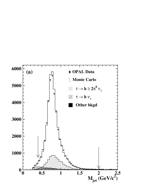
Figure 6: The invariant mass distribution of jets identified as $\tau^{-}\rightarrow h^{-}\,\pi^{0}\nu_{\tau}$ (a) and $\tau^{-}\rightarrow h^{-}\,\geq 2\pi^{0}\nu_{\tau}$ (b). The mass cuts are indicated on the plots. In figure (a) the diagonally hatched area is $\tau^{-}\rightarrow h^{-}\,\geq 2\pi^{0}\nu_{\tau}$ jets, the cross hatched area is $\tau^{-}\rightarrow h^{-}\,\nu_{\tau}$ jets and the dark shaded area is other background. In figure (b) the diagonally hatched area is $\tau^{-}\rightarrow h^{-}\,\pi^{0}\nu_{\tau}$ jets and the cross hatched area is other background.

In the $\tau^{-}\rightarrow h^{-}\,\pi^{0}\nu_{\tau}$ and $\tau^{-}\rightarrow h^{-}\,\geq 2\pi^{0}\nu_{\tau}$ samples the main backgrounds are due to misidentification of other signal channels. In the $\tau^{-}\rightarrow h^{-}\,\pi^{0}\nu_{\tau}$ and the $\tau^{-}\rightarrow h^{-}\,\geq 2\pi^{0}\nu_{\tau}$ samples, the background is reduced by requiring the invariant jet mass to be less than $2.0$ GeV. In the $\tau^{-}\rightarrow h^{-}\,\pi^{0}\nu_{\tau}$ sample, the invariant jet mass is also required to be greater than $0.4$ GeV. The invariant mass distributions of the $\tau^{-}\rightarrow h^{-}\,\pi^{0}\nu_{\tau}$ and $\tau^{-}\rightarrow h^{-}\,\geq 2\pi^{0}\nu_{\tau}$ samples are shown in figure 6.

A number of $\tau^{-}\rightarrow h^{-}\,\pi^{0}\nu_{\tau}$ decays are mistakenly selected into the $\tau^{-}\rightarrow h^{-}\,\geq 2\pi^{0}\nu_{\tau}$ sample. The total energy of the $\pi^{0}$’s from the $\tau^{-}\rightarrow h^{-}\,\pi^{0}\nu_{\tau}$ decays is relatively low and this contamination is reduced by requiring

$$\frac{E_{\pi^{0}}^{\rm total}}{p}>0.8\,,$$

where $E_{\pi^{0}}^{\rm total}$ is the energy sum of all $\pi^{0}$’s identified in the jet and $p$ is the momentum of the primary track.

4 Estimation of $\tau$ backgrounds

The backgrounds from $\rm\tau^{-}\rightarrow e^{-}\,\overline{\nu}_{e}\,\nu_{\tau}$ and $\rm\tau^{-}\rightarrow\mu^{-}\,\overline{\nu}_{\mu}\,\nu_{\tau}$ decays in each sample are measured using distributions previously unused in the selection process. A region in each distribution that is dominated by the background is used to make the measurement. The data and Monte Carlo distributions in the background-dominated region are compared and any deviations between the two are assumed to be caused by the background in question. If the ratio of data to Monte Carlo is different from unity then the Monte Carlo predicted $\tau$ background is rescaled in the background calculation. The error of this correction factor is the combined statistical errors of the data and Monte Carlo. The uncertainties on the correction factors are included in the background errors (including the case where the correction factor is unity).

The $\rm\tau^{-}\rightarrow e^{-}\,\overline{\nu}_{e}\,\nu_{\tau}$ background is estimated using the energy loss (${\rm d}E/{\rm d}x$) in the jet drift chamber. Figure 7 shows the ${\rm d}E/{\rm d}x$ distribution in the data and Monte Carlo for jets with one $\pi^{0}$ and $p<5$ GeV. The ratios of data to Monte Carlo $\rm\tau^{-}\rightarrow e^{-}\,\overline{\nu}_{e}\,\nu_{\tau}$ background jets are calculated using jets that have $9.25<{\rm d}E/{\rm d}x<12.0$ keV/cm. The ratio obtained in each sample is used as a correction factor and is shown in Table 3.

Selection	Background
	$\rm\tau^{-}\rightarrow e^{-}\,\overline{\nu}_{e}\,\nu_{\tau}$	$\rm\tau^{-}\rightarrow\mu^{-}\,\overline{\nu}_{\mu}\,\nu_{\tau}$
$\tau^{-}\rightarrow h^{-}\,\nu_{\tau}$	$1.30\pm 0.18$	$1.39\pm 0.26$
$\tau^{-}\rightarrow h^{-}\,\pi^{0}\nu_{\tau}$	$1.04\pm 0.06$	$0.91\pm 0.28$
$\tau^{-}\rightarrow h^{-}\,\geq 2\pi^{0}\nu_{\tau}$	$0.80\pm 0.28$

Table 3: Correction factors used to scale the $\rm\tau^{-}\rightarrow e^{-}\,\overline{\nu}_{e}\,\nu_{\tau}$ and $\rm\tau^{-}\rightarrow\mu^{-}\,\overline{\nu}_{\mu}\,\nu_{\tau}$ backgrounds.

The $\rm\tau^{-}\rightarrow\mu^{-}\,\overline{\nu}_{\mu}\,\nu_{\tau}$ background in the $\tau^{-}\rightarrow h^{-}\,\nu_{\tau}$ sample is measured by creating a sample of $\rm\tau^{-}\rightarrow\mu^{-}\,\overline{\nu}_{\mu}\,\nu_{\tau}$ jets in both data and Monte Carlo. The efficiency of the muon chamber requirements to reject $\rm\tau^{-}\rightarrow\mu^{-}\,\overline{\nu}_{\mu}\,\nu_{\tau}$ is measured using these samples and the ratio of the efficiencies is used as the Monte Carlo scaling factor for $\rm\tau^{-}\rightarrow\mu^{-}\,\overline{\nu}_{\mu}\,\nu_{\tau}$ background in the $\tau^{-}\rightarrow h^{-}\,\nu_{\tau}$ sample. The $\rm\tau^{-}\rightarrow\mu^{-}\,\overline{\nu}_{\mu}\,\nu_{\tau}$ contamination in the $\tau^{-}\rightarrow h^{-}\,\pi^{0}\nu_{\tau}$ sample is measured by identifying tracks with hits in the muon chambers, since the muon chambers were not used in this selection. The ratio of data to Monte Carlo is used as the scaling factor for $\rm\tau^{-}\rightarrow\mu^{-}\,\overline{\nu}_{\mu}\,\nu_{\tau}$ background in the $\tau^{-}\rightarrow h^{-}\,\pi^{0}\nu_{\tau}$ sample.

Table 4 shows the estimated backgrounds in each selection. In addition to the $\rm\tau^{-}\rightarrow e^{-}\,\overline{\nu}_{e}\,\nu_{\tau}$ and $\rm\tau^{-}\rightarrow\mu^{-}\,\overline{\nu}_{\mu}\,\nu_{\tau}$ decays, there is background from $\tau^{-}\rightarrow h^{-}\,{\rm\overline{K}^{0}\,X\,}\nu_{\tau}$ decays where X is any number of neutral particles in the final state. There is also background from other tau decays, labelled as “Other background” in Table 4, which are mainly tau decays to $\eta$ ($27\%$) and $\omega$ modes ($60\%$), with lesser contributions coming from decays with three charged hadrons in the final state ($13\%$). Both the $\tau^{-}\rightarrow h^{-}\,{\rm\overline{K}^{0}\,X\,}\nu_{\tau}$ and other tau decays are measured from Monte Carlo information. The errors are calculated from the uncertainties in the efficiency matrix and the background branching ratio from the PDG [2]. The background uncertainties in each selection, shown in Table 4, are used in calculating the systematic errors. An additional modelling uncertainty, described in Section 7, is added to the $\tau^{-}\rightarrow h^{-}\,{\rm\overline{K}^{0}\,X\,}\nu_{\tau}$ decays.

Background	Selections
	$\tau^{-}\rightarrow h^{-}\,\nu_{\tau}$	$\tau^{-}\rightarrow h^{-}\,\pi^{0}\nu_{\tau}$	$\tau^{-}\rightarrow h^{-}\,\geq 2\pi^{0}\nu_{\tau}$
$\rm\tau^{-}\rightarrow e^{-}\,\overline{\nu}_{e}\,\nu_{\tau}$	$1.43\pm 0.20\%$	$1.59\pm 0.11\%$	$1.67\pm 0.59\%$
$\rm\tau^{-}\rightarrow\mu^{-}\,\overline{\nu}_{\mu}\,\nu_{\tau}$	$1.57\pm 0.29\%$	$0.68\pm 0.21\%$	$0.02\pm 0.04\%$
$\tau^{-}\rightarrow h^{-}\,{\rm\overline{K}^{0}\,X\,}\nu_{\tau}$	$1.80\pm 0.14\%$	$1.57\pm 0.11\%$	$1.81\pm 0.15\%$
Other background	$0.07\pm 0.02\%$	$0.53\pm 0.03\%$	$3.32\pm 0.24\%$
Total	$4.88\pm 0.38\%$	$4.37\pm 0.26\%$	$6.82\pm 0.65\%$

Table 4: The corrected backgrounds as a percentage of each selection.

5 Branching ratio calculation

The branching ratios are calculated using the information from each selection simultaneously. Each selection can be expressed in terms of the efficiency for detecting each decay mode, the branching ratio of each mode and the number of events selected in the data. For each selection i, the equation is written as

$$\epsilon_{i1}B_{1}+\epsilon_{i2}B_{2}+\epsilon_{i3}B_{3}+\sum_{k=4}^{M}\epsilon_{ik}B_{k}=\frac{N_{i}}{N_{\tau}(1-f^{non-\tau})}$$ (1)

where $\epsilon_{ij}$ ($j=1,3$) are the efficiencies for selecting signal $j$ using selection $i$ and $\epsilon_{ik}$ ($k=4,...$) are the efficiencies for selecting the $\tau$ background modes using selection $i$. $B_{j}$ ($j=1,3$) are the branching ratios of the signal channels and $B_{k}$ ($k=4,...$) are the branching ratios of the backgrounds. $N_{i}$ is the number of data events that pass the selection $i$, $f^{non-\tau}$ is the fraction of non-tau events in the $\tau$-pair sample and $N_{\tau}$ is the total number of data $\tau$’s that pass the $\tau$-pair selection. The selection efficiencies ($\epsilon_{ij}$) for both signal and background are determined from Monte Carlo with the main backgrounds corrected using data distributions (described in section 4). The $\tau$ background branching ratios are taken from the PDG [2] and $f^{non-\tau}$ is shown in Table 2.

The solution of the three simultaneous equations gives the branching ratios in the tau-selected sample. These branching ratios are then corrected to account for the biases introduced to the $\tau$-pair sample by the $\tau$-pair selection. These factors are $0.989\pm 0.002$, $1.019\pm 0.001$ and $1.013\pm 0.002$ for the $\tau^{-}\rightarrow h^{-}\,\nu_{\tau}$  $\tau^{-}\rightarrow h^{-}\,\pi^{0}\nu_{\tau}$ and $\tau^{-}\rightarrow h^{-}\,\geq 2\pi^{0}\nu_{\tau}$ decays, respectively.

6 Results

The $\tau$-pair selection identifies $190728$ $\tau$ candidates. The selections for $\tau^{-}\rightarrow h^{-}\,\nu_{\tau}$, $\tau^{-}\rightarrow h^{-}\,\pi^{0}\nu_{\tau}$ and $\tau^{-}\rightarrow h^{-}\,\geq 2\pi^{0}\nu_{\tau}$ yield $18547$, $40537$ and $6802$ events respectively. The efficiencies for detecting these signals are listed in Table 5.

Selection	Selection efficiency from MC
	$\tau^{-}\rightarrow h^{-}\,\nu_{\tau}$	$\tau^{-}\rightarrow h^{-}\,\pi^{0}\nu_{\tau}$	$\tau^{-}\rightarrow h^{-}\,\geq 2\pi^{0}\nu_{\tau}$
$0\pi^{0}$	$0.5502\pm 0.0024$	$0.1003\pm 0.0010$	$0.0249\pm 0.0008$
$1\pi^{0}$	$0.0455\pm 0.0010$	$0.5985\pm 0.0016$	$0.4273\pm 0.0025$
$\geq 2\pi^{0}$	$0.0005\pm 0.0001$	$0.0237\pm 0.0005$	$0.2730\pm 0.0023$

Table 5: Efficiencies for identifying the signals for each selection. The errors on these efficiencies are based on Monte Carlo statistics only.

The efficiency for detecting $\tau^{-}\rightarrow h^{-}\,\nu_{\tau}$ is an average of the efficiencies for selecting $\tau^{-}\rightarrow\pi^{-}\,\nu_{\tau}$ and $\tau^{-}\rightarrow{\rm K^{-}}\,\nu_{\tau}$ weighted by their relative branching ratios. Similarly, the efficiency for detecting $\tau^{-}\rightarrow h^{-}\,\pi^{0}\nu_{\tau}$ is an average of the efficiencies for selecting $\tau^{-}\rightarrow\pi^{-}\,\pi^{0}\nu_{\tau}$ and $\tau^{-}\rightarrow{\rm K^{-}}\,\pi^{0}\nu_{\tau}$ weighted by their relative branching ratios. The same method is used for the $\tau^{-}\rightarrow h^{-}\,\geq 2\pi^{0}\nu_{\tau}$ efficiency where the decay modes are listed in Table 1.

The backgrounds in the $\tau^{-}\rightarrow h^{-}\,\nu_{\tau}$, $\tau^{-}\rightarrow h^{-}\,\pi^{0}\nu_{\tau}$ and $\tau^{-}\rightarrow h^{-}\,\geq 2\pi^{0}\nu_{\tau}$ samples are given in Table 4. The branching ratios for $\tau^{-}\rightarrow h^{-}\,\nu_{\tau}$, $\tau^{-}\rightarrow h^{-}\,\pi^{0}\nu_{\tau}$, and $\tau^{-}\rightarrow h^{-}\,\geq 2\pi^{0}\nu_{\tau}$ are calculated using the method described in section 5 and the results are shown in Table 6.

Channel	Branching Ratio ($\%$)
$\tau^{-}\rightarrow h^{-}\,\nu_{\tau}$	$\rm{11.98\pm 0.13\pm 0.16}$
$\tau^{-}\rightarrow h^{-}\,\pi^{0}\nu_{\tau}$	$\rm{25.89\pm 0.17\pm 0.29}$
$\tau^{-}\rightarrow h^{-}\,\geq 2\pi^{0}\nu_{\tau}$	$\rm{9.91\pm 0.31\pm 0.27}$

Table 6: Branching ratio results. The first error is statistical and the second systematic.

The measurements of these branching ratios are correlated. The correlation coefficients between branching ratios calculated using the statistical errors on each branching ratio are given in Table 7.

Sample	$\tau^{-}\rightarrow h^{-}\,\pi^{0}\nu_{\tau}$	$\tau^{-}\rightarrow h^{-}\,\geq 2\pi^{0}\nu_{\tau}$
$\tau^{-}\rightarrow h^{-}\,\nu_{\tau}$	$-0.430$	$0.167$
$\tau^{-}\rightarrow h^{-}\,\pi^{0}\nu_{\tau}$		$-0.470$

Table 7: The correlation coefficients between each measurement.

7 Systematic errors

The systematic errors on the branching ratios are shown in Table 8.

	Systematic error for each selection (%)
	$\tau^{-}\rightarrow h^{-}\,\nu_{\tau}$	$\tau^{-}\rightarrow h^{-}\,\pi^{0}\nu_{\tau}$	$\tau^{-}\rightarrow h^{-}\,\geq 2\pi^{0}\nu_{\tau}$
MC statistics	$0.11$	$0.17$	$0.14$
$a_{1}$ modelling	$0.01$	$0.13$	$0.15$
1-cluster $\pi^{0}$ threshold	$0.03$	$0.02$	$0.03$
2-cluster $\pi^{0}$ threshold	$0.03$	$0.11$	$0.11$
Anode plane cut	$0.00$	$0.05$	$0.03$
Photon conversions	$0.06$	$0.03$	$0.02$
Energy smearing	$0.01$	$0.01$	$0.03$
Radiative clusters	$0.03$	$0.00$	$0.00$
Energy scale	$0.03$	$0.03$	$0.04$
Signal BR uncertainty	$0.01$	$0.05$	$0.03$
Bias factors	$0.02$	$0.03$	$0.02$
Unmodelled channels	$0.00$	$0.02$	$0.04$
Non-$\tau$ backgrounds	$0.02$	$0.04$	$0.01$
$\rm\tau^{-}\rightarrow e^{-}\,\overline{\nu}_{e}\,\nu_{\tau}$	$0.04$	$0.07$	$0.08$
$\rm\tau^{-}\rightarrow\mu^{-}\,\overline{\nu}_{\mu}\,\nu_{\tau}$	$0.05$	$0.08$	$0.01$
$\tau^{-}\rightarrow h^{-}\,{\rm\overline{K}^{0}\,X\,}\nu_{\tau}$	$0.06$	$0.07$	$0.04$
Other backgrounds	$0.00$	$0.03$	$0.03$
Total	$0.16$	$0.29$	$0.27$

Table 8: Systematic errors.

The efficiencies for detecting the signals and backgrounds are taken from Monte Carlo and special attention is paid to the Monte Carlo modelling. The first half of Table 8 gives the systematic errors due to aspects of the analysis such as Monte Carlo modelling of hadronic showers, track finding, conversion finding, radiative photons and energy scale. The second half of Table 8 gives the systematic errors due to the backgrounds. We briefly describe the individual contributions to the systematic errors.

The $a_{1}\rightarrow\pi^{-}2\pi^{0}$ decay was simulated using the IMR model, as described in section 3. The IMR model gives a better description of the $a_{1}^{-}\rightarrow\pi^{-}\pi^{+}\pi^{-}$ data primarily because of the inclusion of the polynomial background term [12]. The uncertainty in the contribution of the polynomial background was measured in [10] to be approximately $17\%$. The systematic error in the branching ratios due to the uncertainty in the $a_{1}$ model is conservatively estimated by varying the normalization of the polynomial background by $\pm 50\%$ ($3\sigma$).

The Monte Carlo models the hadronic showering in $\tau$ decays reasonably well. The thresholds for the neutral clusters, one-cluster and two-cluster $\pi^{0}$’s, as well as other requirements, have been carefully studied to avoid any poorly modelled regions due to low energy hadronic clusters. However, as the energy thresholds are lowered, deviations between the data and Monte Carlo appear since clusters close to the track from hadronic interactions are accepted into the $\pi^{0}$-finding algorithm. The lower energy thresholds of both the one and two cluster $\pi^{0}$ cases are varied to estimate the systematic error due to the Monte Carlo modelling of energy deposition in the electromagnetic calorimeter. The lower energy threshold of the one-cluster $\pi^{0}$ case is varied from $2.0$ to $3.0$ GeV and the energy threshold of the two-cluster $\pi^{0}$ case is varied from $2.6$ to $4.0$ GeV. The maximum variation from each nominal branching ratio is taken as the systematic error in each case.

The effect of tracks passing close to the anode plane of the OPAL jet chamber is considered as a source of systematic error. The Monte Carlo does not perfectly model the position of tracks close to the anode plane. The branching ratios were recalculated by removing tracks within $0.25^{\circ}$ of the anode plane. The resulting change in the branching ratios is taken as the systematic error.

Approximately $5\%$ of the identified $\pi^{0}$’s are composed of a neutral cluster and a photon conversion. Although the Monte Carlo does a reasonable job of modelling conversions, there are minor discrepancies between data and Monte Carlo. The ratio of data to Monte Carlo jets with an identified conversion pair is found to be $0.985\pm 0.013$. The branching ratios are calculated with Monte Carlo jets containing a conversion weighted to simulate a $\pm 3\sigma$ ($\pm 4\%$) change in conversion identification efficiency. The maximum variation from each nominal branching ratio is taken as the systematic error. The sensitivity of the results to photon conversions is also checked by dropping the conversion routine and recalculating the branching ratios.

The energy of each electromagnetic calorimeter cluster in the Monte Carlo is smeared. The uncertainty due to this smearing is assessed by varying the amount of smearing applied by $\pm 20\%$. The change in the branching ratios is taken as the systematic error.

Clusters were considered to be due to radiative photons if the mass of the track and cluster was greater than $3$ GeV. These clusters are ignored by the $\pi^{0}$-algorithm. This requirement was removed and the change in the branching ratios was taken as the systematic error.

The energy scale uncertainty reflects the uncertainty in the electromagnetic calorimeter calibration between Monte Carlo and data. To determine the systematic uncertainty the clusters are rescaled by $\pm 0.2\%$ and the largest effect on the branching ratios is taken as the systematic uncertainty.

The selection efficiencies depend on the relative branching ratios of the individual decay modes. The signal branching ratios were calculated using the PDG branching ratios and uncertainties [2]. The dependence of the efficiency and the decay branching ratios on the signal branching ratios was evaluated and included as a systematic uncertainty.

A small correction must be applied to the branching ratios to correct the slight bias introduced by the $\tau$-pair selection criteria. The dependence of the bias factor on the $\tau$-pair selection and on the branching ratios of each channel is found to be relatively small. In addition, other Monte Carlo samples using a different electromagnetic shower model give similar results. The systematic error on each branching ratio is calculated directly using the bias factor error.

The Monte Carlo used in this analysis did not include some decay modes defined as signals by the PDG [2]. Table 1 shows these decay modes. The systematic effect of the $\tau^{-}\rightarrow h^{-}\,4\pi^{0}\nu_{\tau}$ mode on the $\tau^{-}\rightarrow h^{-}\,\pi^{0}\nu_{\tau}$ and $\tau^{-}\rightarrow h^{-}\,\geq 2\pi^{0}\nu_{\tau}$ samples is calculated using the PDG branching ratio and the assumption that the efficiency for $\tau^{-}\rightarrow h^{-}\,4\pi^{0}\nu_{\tau}$ is the same as that for $\tau^{-}\rightarrow h^{-}\,3\pi^{0}\nu_{\tau}$. The uncertainty for each of these modes is assumed to be $50\%$ of their respective branching ratios. The total systematic error is calculated from these uncertainties.

The systematic errors on the branching ratios due to non-$\tau$ and $\tau$ backgrounds are calculated from the uncertainties given in Tables 2 and 4, respectively. An additional error has been added to the $\tau^{-}\rightarrow h^{-}\,{\rm\overline{K}^{0}\,X\,}\nu_{\tau}$ decays to account for any uncertainty in the energy deposited by a neutral hadron in the electromagnetic calorimeter. A 10% error was added to the $\tau^{-}\rightarrow h^{-}\,{\rm\overline{K}^{0}\,X\,}\nu_{\tau}$ background in the $\tau^{-}\rightarrow h^{-}\,\nu_{\tau}$ sample. A second error was added to the $\tau^{-}\rightarrow h^{-}\,{\rm\overline{K}^{0}\,X\,}\nu_{\tau}$ background in all three samples to account for possible migration of the background from one $\pi^{0}$ sample to another.

8 Discussion

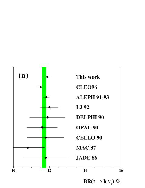
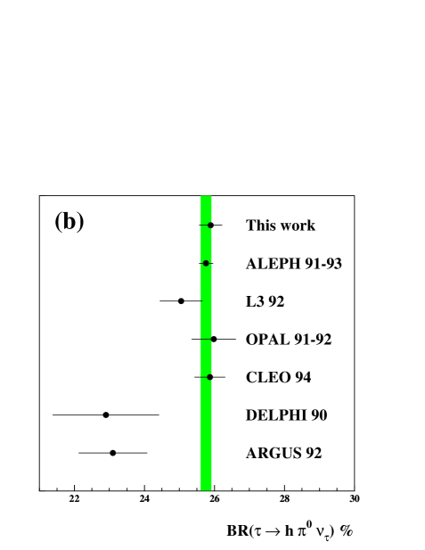
Figure 8: The branching ratios for the $\tau^{-}\rightarrow h^{-}\,\nu_{\tau}$ and $\tau^{-}\rightarrow h^{-}\,\pi^{0}\nu_{\tau}$ decay modes for this work are compared with previous measurements. The solid band in each plot is the PDG average for that channel. The PDG average for the $\tau^{-}\rightarrow h^{-}\,\nu_{\tau}$ branching ratio does not include the CLEO measurement while the PDG average for the $\tau^{-}\rightarrow h^{-}\,\pi^{0}\nu_{\tau}$ branching ratio uses all of the measurements. The error bars shown include both systematic and statistical uncertainties.

The $\tau^{-}\rightarrow h^{-}\,\nu_{\tau}$ branching ratio is measured to be $(11.98\pm 0.13\pm 0.16)\,\%$ and is compared with other published results in figure 8. The $\tau^{-}\rightarrow h^{-}\,\nu_{\tau}$ branching ratio agrees well with the PDG world average of $(11.70\pm 0.11)\%$ [2] but is slightly above the recent CLEO measurement of $(11.52\pm 0.13)\%$ [17] and the theoretical prediction of $(11.65\pm 0.06)\%$ made by Decker and Finkemeier [18].

The $\tau^{-}\rightarrow h^{-}\,\nu_{\tau}$ branching ratio can be used to measure the ratio of the charged current coupling constants of taus and muons. Lepton universality requires that the weak charged current gauge coupling strengths be identical: $g_{e}=g_{\mu}=g_{\tau}$. The $g_{\mu}/g_{\tau}$ ratio is probed by comparing the decays $h^{-}\rightarrow\mu^{-}\overline{\nu}_{\mu}$ and $\tau^{-}\rightarrow h^{-}\,\nu_{\tau}$. An expression for $g_{\tau}^{2}/g_{\mu}^{2}$ is given by

$${\frac{g_{\tau}^{2}}{g_{\mu}^{2}}}=\left\{\frac{2m^{2}_{\mu}}{m^{2}_{\tau}}\right\}\frac{{\rm BR}(\tau^{-}\rightarrow h^{-}\,\nu_{\tau})}{H_{\pi}+H_{\rm K}}\,,$$

where

$$H_{h}=(1+\delta_{h})\left(\frac{\tau_{\tau}m_{\tau}}{\tau_{h}m_{h}}\right)\left[\frac{1-\left(m_{h}/m_{\tau}\right)^{2}}{1-\left(m_{\mu}/m_{h}\right)^{2}}\right]^{2}{\rm BR}\,(h^{-}\rightarrow\mu^{-}\overline{\nu}_{\mu})\,,$$

and $\delta_{h}$ is an electromagnetic radiative correction [18]. The $\pi^{-}\rightarrow\mu^{-}\overline{\nu}_{\mu}$ and ${\rm K^{-}}\rightarrow\mu^{-}\overline{\nu}_{\mu}$ branching ratios, the masses of the tau, muon and the pion, and the lifetime of the pion are taken from the PDG [2]. The ratio $g_{\tau}/g_{\mu}$ is found to be

$${\frac{g_{\tau}}{g_{\mu}}}=1.018\pm 0.010\,,$$

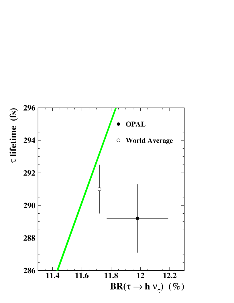
Figure 9: The tau lifetime is plotted as a function of $\tau^{-}\rightarrow h^{-}\,\nu_{\tau}$ branching ratio. The shaded band shows the Standard Model prediction assuming lepton universality and its width reflects the uncertainty associated with the tau mass. The solid point uses the $\tau^{-}\rightarrow h^{-}\,\nu_{\tau}$ branching ratio obtained in this measurement and the OPAL tau lifetime. The open circle uses the world average for both the $\tau^{-}\rightarrow h^{-}\,\nu_{\tau}$ branching ratio and tau lifetime.

where the error on $g_{\tau}/g_{\mu}$ is dominated by the uncertainties in the $\tau^{-}\rightarrow h^{-}\,\nu_{\tau}$ branching ratio and the OPAL $\tau$ lifetime [19]. The point in figure 9 shows the result from this work plotted against the $\tau$ lifetime. The Standard Model prediction is shown as the shaded band with a width reflecting the uncertainty in $m_{\tau}$. If we recalculate the world average $\tau^{-}\rightarrow h^{-}\,\nu_{\tau}$ branching ratio including our result and use the PDG value for the tau lifetime [2], then the ratio $g_{\tau}/g_{\mu}$ is found to be $1.003\pm 0.005$.

The ratio of $g_{\tau}/g_{\mu}$ can also be measured by comparing the $\rm\tau^{-}\rightarrow e^{-}\,\overline{\nu}_{e}\,\nu_{\tau}$ and $\rm\mu\rightarrow e^{-}\overline{\nu}_{e}\nu_{\mu}$ decays. Using the PDG values for the $\rm\tau^{-}\rightarrow e^{-}\,\overline{\nu}_{e}\,\nu_{\tau}$ and $\tau$ lifetime gives $g_{\tau}/g_{\mu}=1.000\pm 0.003$. Although this result is more precise, the two measurements are complementary. The measurement using the $\tau^{-}\rightarrow\pi^{-}\,\nu_{\tau}$ and $\pi^{-}\rightarrow\mu^{-}\overline{\nu}_{\mu}$ decays probes the couplings to a longitudinal W boson, while the measurement using the $\rm\tau^{-}\rightarrow e^{-}\,\overline{\nu}_{e}\,\nu_{\tau}$ and $\rm\mu\rightarrow e^{-}\overline{\nu}_{e}\nu_{\mu}$ decays probes the couplings to a transverse W.

The decay $\tau^{-}\rightarrow h^{-}\nu_{\tau}$ is also sensitive to the presence of physics beyond the minimal Standard Model. As an example, in $R$-parity violating (RPV) extensions of supersymmetric models [20] $\tau^{-}\rightarrow h^{-}\nu_{\tau}$ and ${h^{-}}\rightarrow\mu^{-}\bar{\nu}_{\mu}$ receive an additional contribution from the exchange of a right-handed scalar d-type quark, $\tilde{\mathrm{d}}^{k}_{R}$, where $k$ is a family index. This exchange can be cast in a $V-A\otimes V-A$ form leading to a modification of the Standard Model predicted couplings by a term proportional to $|\mbox{$\lambda^{\prime}_{ijk}$}|^{2}/\mbox{$m^{2}(\tilde{\mathrm{d}}^{k}_{R})$}$ as outlined in [21]. The RPV Yukawa couplings probed by $\tau^{-}\rightarrow h^{-}\nu_{\tau}$ and ${h^{-}}\rightarrow\mu^{-}\bar{\nu}_{\mu}$ decays are $\lambda^{\prime}_{31k}$ and $\lambda^{\prime}_{21k}$ respectively. Note that, under the assumption that only one RPV Yukawa coupling is non-zero, the decays $\tau^{-}\rightarrow\mathrm{K}^{-}\nu_{\tau}$ and ${\rm K^{-}}\rightarrow\mu^{-}\bar{\nu}_{\mu}$ are unaffected by RPV since they involve products of two different coupling constants.

Using the formalism developed in [21], limits can be set on $\lambda^{\prime}_{31k}$ and $\lambda^{\prime}_{21k}$ from the expression, derived here for the first time,

$$\frac{|\mbox{$\lambda^{\prime}_{31k}$}|^{2}-|\mbox{$\lambda^{\prime}_{21k}$}|^{2}}{\mbox{$m^{2}(\tilde{\mathrm{d}}^{k}_{R})$}}=2\sqrt{2}G_{\mathrm{F}}V_{\mathrm{ud}}\left[\frac{2\mbox{$m_{\mu}$}^{2}}{m_{\tau}^{2}}\frac{\mathrm{BR}(\mbox{$\tau^{-}\rightarrow h^{-}\nu_{\tau}$})}{H_{\pi}}-1-\frac{H_{K}}{H_{\pi}}\right].$$

Making the assumption that only one Yukawa coupling is non-zero leads to the following 95% confidence level limits, calculated using $m(\tilde{\mathrm{d}}^{k}_{R})$ = 100 GeV, of

$$|\mbox{$\lambda^{\prime}_{31k}$}|<0.15\;\;\;\mbox{\rm and}\;\;\;|\mbox{$\lambda^{\prime}_{21k}$}|<0.09$$

using the OPAL $\tau^{-}\rightarrow h^{-}\,\nu_{\tau}$ and tau lifetime [19] measurements and

$$|\mbox{$\lambda^{\prime}_{31k}$}|<0.09\;\;\;\mbox{\rm and}\;\;\;|\mbox{$\lambda^{\prime}_{21k}$}|<0.07$$

using the world average $\tau^{-}\rightarrow h^{-}\nu_{\tau}$ branching ratio and tau lifetime. Previous measurements have quoted the 68% ($1\sigma$) confidence limits [22]. Using the OPAL measurements, the 68% ($1\sigma$) confidence limits are $|\mbox{$\lambda^{\prime}_{31k}$}|<0.13$ and $|\mbox{$\lambda^{\prime}_{21k}$}|<0.06$, while the world average results give 68% confidence limits of $|\mbox{$\lambda^{\prime}_{31k}$}|<0.07$ and $|\mbox{$\lambda^{\prime}_{21k}$}|<0.05$. The limit on $\lambda^{\prime}_{21k}$ set using this method is competitive with the present best limit derived from pion decay to electrons and muons [21]. Limits on $\lambda^{\prime}_{31k}$ have been obtained previously using the decay $\tau^{-}\rightarrow\pi^{-}\nu_{\tau}$  [22]. Our new calculation using $\tau^{-}\rightarrow h^{-}\nu_{\tau}$ has several advantages over this method. Firstly, BR($\tau^{-}\rightarrow h^{-}\nu_{\tau}$) is more precisely known than BR($\tau^{-}\rightarrow\pi^{-}\nu_{\tau}$). Additionally, BR($\tau^{-}\rightarrow h^{-}\nu_{\tau}$) is a directly measured quantity making the limits more experimentally compelling than those derived from $\tau^{-}\rightarrow\pi^{-}\nu_{\tau}$.

The $\tau^{-}\rightarrow h^{-}\,\pi^{0}\nu_{\tau}$ branching ratio is measured to be $(25.89\pm 0.17\pm 0.29)\,\%$ and is compared to other published branching ratios in figure 8. Some of the branching ratios shown have been corrected by the PDG in order to treat the kaon backgrounds in a uniform manner. The $\tau^{-}\rightarrow h^{-}\,\pi^{0}\nu_{\tau}$ branching ratio result measured in this work agrees well with the PDG average ($25.76\pm 0.15\%$) and the previous measurements.

The Conserved Vector Current hypothesis [23] can be used to predict the $\tau^{-}\rightarrow\pi^{-}\,\pi^{0}\nu_{\tau}$ branching ratio from low energy ${\rm e^{+}e^{-}}\rightarrow\,\pi^{+}\pi^{-}$ data. A number of predictions for the $\tau^{-}\rightarrow\pi^{-}\,\pi^{0}\nu_{\tau}$ branching ratio have been made [11, 24]. A recent review by Eidelman and Ivanchenko [25] predicted the branching ratio to be $(24.25\pm 0.77)\%$. The $\tau^{-}\rightarrow h^{-}\,\pi^{0}\nu_{\tau}$ branching ratio measured in this work should be modified by subtracting the $\tau^{-}\rightarrow{\rm K^{-}}\,\pi^{0}\nu_{\tau}$ branching ratio [2] giving a $\tau^{-}\rightarrow\pi^{-}\,\pi^{0}\nu_{\tau}$ branching ratio of $(25.73\pm 0.31)\%$. The result measured here is consistent (within two standard deviations) with the CVC prediction.

The $\tau^{-}\rightarrow h^{-}\,\geq 2\pi^{0}\nu_{\tau}$ branching ratio is measured to be $(9.91\pm 0.31\pm 0.27)\,\%$, in comparison to the PDG average for the $\tau^{-}\rightarrow h^{-}\,\geq 2\pi^{0}\nu_{\tau}$ branching ratio of $(10.48\pm 0.35)\%$ [2]. The PDG number quoted is the sum of the average values for the branching ratios of the tau decay to the $h^{-}2\pi^{0}\nu_{\tau}$, $h^{-}3\pi^{0}\nu_{\tau}$, $h^{-}4\pi^{0}\nu_{\tau}$, $\pi^{-}\overline{K}^{0}\nu_{\tau}$ and $K^{-}\overline{K}^{0}\nu_{\tau}$ modes.

9 Conclusions

The branching ratios of $\tau^{-}\rightarrow h^{-}\,\nu_{\tau}$, $\tau^{-}\rightarrow h^{-}\,\pi^{0}\nu_{\tau}$ and $\tau^{-}\rightarrow h^{-}\,\geq 2\pi^{0}\nu_{\tau}$ decays have been measured with the OPAL detector at LEP. The branching ratios are

BR($\tau^{-}\rightarrow h^{-}\,\nu_{\tau}$)	=	$(11.98\pm 0.13\pm 0.16)\,\%$
BR($\tau^{-}\rightarrow h^{-}\,\pi^{0}\nu_{\tau}$)	=	$(25.89\pm 0.17\pm 0.29)\,\%$
BR($\tau^{-}\rightarrow h^{-}\,\geq 2\pi^{0}\nu_{\tau}$)	=	$(9.91\pm 0.31\pm 0.27)\,\%$	,

where the first error is statistical and the second error is systematic. These new measurements are more precise than previous OPAL measurements and supersede those results.

The $\tau^{-}\rightarrow h^{-}\,\nu_{\tau}$ branching ratio measured in this work is found to be in good agreement with previous measurements. The ratio of the charged current coupling constants of muons and taus using the $\tau^{-}\rightarrow h^{-}\,\nu_{\tau}$ branching ratio is found to be $g_{\mu}/g_{\tau}=(1.018\pm 0.010)$, consistent with lepton universality. The $\tau^{-}\rightarrow h^{-}\,\nu_{\tau}$ branching ratio is used to place limits on supersymmetric $R$-parity violating Yukawa couplings. The $\tau^{-}\rightarrow h^{-}\,\pi^{0}\nu_{\tau}$ branching ratio found in this work is in good agreement with the previous results and also with the Conserved Vector Current prediction. Finally, the $\tau^{-}\rightarrow h^{-}\,\geq 2\pi^{0}\nu_{\tau}$ branching ratio measured in this work is found to be consistent with the current PDG world average.

Acknowledgements
We particularly wish to thank the SL Division for the efficient operation of the LEP accelerator at all energies and for their continuing close cooperation with our experimental group. We thank our colleagues from CEA, DAPNIA/SPP, CE-Saclay for their efforts over the years on the time-of-flight and trigger systems which we continue to use. In addition to the support staff at our own institutions we are pleased to acknowledge the
Department of Energy, USA,
National Science Foundation, USA,
Particle Physics and Astronomy Research Council, UK,
Natural Sciences and Engineering Research Council, Canada,
Israel Science Foundation, administered by the Israel Academy of Science and Humanities,
Minerva Gesellschaft,
Benoziyo Center for High Energy Physics,
Japanese Ministry of Education, Science and Culture (the Monbusho) and a grant under the Monbusho International Science Research Program,
German Israeli Bi-national Science Foundation (GIF),
Bundesministerium für Bildung, Wissenschaft, Forschung und Technologie, Germany,
National Research Council of Canada,
Research Corporation, USA,
Hungarian Foundation for Scientific Research, OTKA T-016660, T023793 and OTKA F-023259.

Figure 1: The distribution of the number of neutral clusters per jet for one-prong selected jets. The distribution is shown in both a linear vertical scale (left plot) and a logarithmic vertical scale (right plot).

Figure 2: The distribution of the energy of clusters identified as radiative photons.

Figure 3: (a) The invariant mass distribution of two neutral clusters in data and Monte Carlo for jets with two neutral clusters with energy between $0.5$ and $9.0$ GeV. (b) The invariant mass distribution for the neutral cluster pairs selected by the $\pi^{0}$ algorithm.

Figure 4: (a) The distribution of the number of $\pi^{0}$’s in each one-prong jet identified by the $\pi^{0}$ finding algorithm. (b) The distribution of the types of $\pi^{0}$’s identified in one-prong jets.

Figure 5: The energy distribution of reconstructed $\pi^{0}$’s shown in both linear and logarithmic scales. (a) and (b) show the energy of $\pi^{0}$’s in $\tau^{-}\rightarrow h^{-}\,\pi^{0}\nu_{\tau}$ jets. (c) and (d) show the energy of $\pi^{0}$’s in $\tau^{-}\rightarrow h^{-}\,\geq 2\pi^{0}\nu_{\tau}$ jets. The structure observed at 9 GeV corresponds to the one-cluster $\pi^{0}$ threshold.

Figure 7: The ${\rm d}E/{\rm d}x$ distribution used to measure the $\rm\tau^{-}\rightarrow e^{-}\,\overline{\nu}_{e}\,\nu_{\tau}$ background in the $\tau^{-}\rightarrow h^{-}\,\pi^{0}\nu_{\tau}$ sample. A background-dominated region is created by selecting jets with $9.25<{\rm d}E/{\rm d}x<12.0$ keV/cm (indicated on the histogram). The cross hatched region corresponds to the $\rm\tau^{-}\rightarrow e^{-}\,\overline{\nu}_{e}\,\nu_{\tau}$ background events.

References

- [1] A. Pich, Nucl. Phys. Proc. Suppl. 55C (1997) 3.
- [2] R. M. Barnett et al., Particle Data Group, Phys. Rev. D54 (1996) 1.
- [3] OPAL Collab., K. Ahmet et al., Nucl. Instrum. and Meth. A305 (1991) 275.
-
[4]
P. P. Allport et al., Nucl. Instrum. and Meth. A324 (1993) 34;
P. P. Allport et al., Nucl. Instrum. and Meth. A346 (1994) 476. - [5] M. Hauschild et al., Nucl. Instrum. and Meth. A314 (1992) 74.
- [6] S. Jadach, B.F.L. Ward and Z. Wa̧s, Comp. Phys. Comm. 79 (1994) 503.
- [7] S. Jadach, Z. Wa̧s, R. Decker and J. H. Kühn, Comp. Phys. Comm. 76 (1993) 361.
- [8] R. Brun et al., GEANT 3, Report DD/EE/84-1, CERN (1989).
- [9] J. Allison et al., Nucl. Instrum. and Meth. A317 (1992) 47.
- [10] OPAL Collab., K. Ackerstaff et al., Z.Phys. C75 (1997) 593.
- [11] J. H. Kühn and A. Santamaria, Z. Phys. C48 (1990) 445.
- [12] N. Isgur, C. Morningstar and C. Reader, Phys. Rev. D39 (1989) 1357.
- [13] OPAL Collab., G. Alexander et al., Z. Phys. C52 (1991) 175.
- [14] OPAL Collab., G. Alexander et al., Phys. Lett. B369 (1996) 163.
- [15] OPAL Collab., G. Alexander et al., Z. Phys. C70 (1996) 357.
- [16] OPAL Collab., R. Akers et al., Phys. Lett. B328 (1994) 207.
- [17] CLEO Collab., A. Anastassov et al., Phys.Rev.D55 (1997) 2559.
-
[18]
R. Decker and M. Finkemeier,
Phys. Lett. B316 (1993) 403;
R. Decker and M. Finkemeier, Phys. Lett. B334 (1994) 199. - [19] OPAL Collab., G. Alexander et al., Phys. Lett. B374 (1996) 341.
-
[20]
S. Weinberg, Phys. Rev. D26 (1982) 287;
N. Sakai and T. Yanagida, Nucl. Phys. B197 (1982) 533. - [21] V. Barger, G.F. Giudice and T. Han, Phys. Rev. D40 (1989) 2987.
-
[22]
G. Bhattacharyya and D. Choudhury, Mod. Phys. Lett. A10 (1995) 1699;
G. Bhattacharyya, “A Brief Review of R-Parity Violating Couplings”, presented at the workshop on Physics Beyond the Standard Model: Beyond the Desert: Accelerator and Nonaccelerator Approaches, Tegernsee, Germany, 8-14 Jun 1997 (Hep-ph/9709395). - [23] R. Feynman and M. Gell-Mann, Phys. Rev. 109 (1958) 193.
-
[24]
Yung-Su Tsai, Phys. Rev. D4 (1971) 2821;
F. J. Gilman and S.H. Rhie, Phys. Rev. D31 (1985) 1066;
S. I. Eidelman and V. N. Ivanchenko, Phys. Lett. B257 (1991) 437;
W.J. Marciano, Phys. Rev. D45 (1992) 721;
R. J. Sobie, Z. Phys. C65 (1995) 79. - [25] S. I. Eidelman and V. N. Ivanchenko. Nucl. Phys. Proc. Suppl. 55C (1997) 181.