Direct Measurement of the Top Quark Mass at DØ

Abstract

We determine the top quark mass $m_{t}$ using $t\overline{t}$ pairs produced in the DØ detector by $\sqrt{s}=1.8\ \text{TeV}$ $p\overline{p}$ collisions in a $125\ \text{pb}^{-1}$ exposure at the Fermilab Tevatron. We make a two constraint fit to $m_{t}$ in $t\overline{t}\rightarrow bW^{+}\overline{b}W^{-}$ final states with one $W$ boson decaying to $q\overline{q}$ and the other to $e\nu$ or $\mu\nu$. Likelihood fits to the data yield $m_{t}(l+\text{jets})=173.3\pm 5.6\ \textrm{(stat)}\pm 5.5\ \textrm{(syst)}\ \text{GeV}/c^{2}$. When this result is combined with an analysis of events in which both $W$ bosons decay into leptons, we obtain $m_{t}=172.1\pm 5.2\ \textrm{(stat)}\pm 4.9\ \textrm{(syst)}\ \text{GeV}/c^{2}$. An alternate analysis, using three constraint fits to fixed top quark masses, gives $m_{t}(l+\text{jets})=176.0\pm 7.9\ \textrm{(stat)}\pm 4.8\ \textrm{(syst)}\ \text{GeV}/c^{2}$, consistent with the above result. Studies of kinematic distributions of the top quark candidates are also presented.

Contents

toc

I Introduction

The discovery of the top quark by the CDF [3] and DØ [4] collaborations at the Fermilab Tevatron ended the search phase of top quark physics. Since then, emphasis has shifted to determining its properties — especially its large mass (about 200 times that of a proton) and production cross section. Reviews of searches for and the initial observations of the top quark are given in Ref. [5]. Details of the initial DØ top quark search can be found in Ref. [6]. This paper reports on the determination of the top quark mass using all the data collected by the DØ experiment during the 1992–1996 Tevatron runs. This is more than twice as much data as was available for the initial observation. In addition, improvements have been made in event selection, object reconstruction, and mass analysis techniques. The result is a reduction of the statistical and systematic errors by nearly a factor of four. A short paper giving results from this analysis has been published [7].

The top quark is one of the fundamental fermions in the standard model of electroweak interactions and is the weak-isospin partner of the bottom quark. For a top quark with mass substantially greater than that of the $W$ boson, the standard model predicts it to decay promptly (before hadronization) to a $W$ boson plus a bottom quark with a branching fraction of nearly $100\%$. A precision measurement of the top quark mass, along with the $W$ boson mass and other electroweak data, can set constraints on the mass of the standard model Higgs boson. It may also be helpful in understanding the origin of quark masses.

In $p\overline{p}$ collisions at a $1.8\ \text{TeV}$ center of mass energy, top quarks are produced primarily as $t\overline{t}$ pairs. Each decays into a $W$ boson plus a bottom quark, resulting in events having several jets and often a charged lepton. Due to the large top quark mass, these final state objects tend to have large momenta transverse to the $p\overline{p}$ direction. About $30\%$ of $t\overline{t}$ decays have a single electron or muon (from the decay of one of the $W$ bosons) with a large transverse momentum. Typically, the neutrino that accompanies this electron or muon will also have a large transverse momentum, producing significant missing transverse energy. These characteristics allow for the selection of a sample of “lepton + jets” events with an enriched signal to background ratio. This sample is the basis for the top quark mass analysis reported in this paper. It also comprises a large portion of the data sample used for the measurement of the $p\overline{p}\rightarrow t\overline{t}$ production cross section [8]. A similar mass analysis for the final state with two charged leptons plus jets is described in Ref. [9].

Three methods have been used to determine the top quark mass in the lepton + jets channels. Two of them use constrained variable-mass kinematic fits to obtain a best-fit mass value for each event. The top quark mass is then extracted using a maximum likelihood fit to a two-dimensional distribution, with one axis being the best-fit mass, and the other being a variable which discriminates $t\overline{t}$ events from the expected backgrounds. The difference between these two methods is in the discriminant variable and the binning used. The third method uses $\chi^{2}$ values from fixed-mass kinematic fits. A cut is made using a top quark discriminant to select a sample of events with low background. The expected contribution from the background is subtracted from the distribution of $\chi^{2}$ versus mass, and the resulting background-subtracted distribution is fit near the minimum to extract the top quark mass.

This paper is organized as follows. Section II briefly describes aspects of the DØ detector essential for this analysis. Section III discusses event selection, including triggers, particle identification, and the criteria used to select the initial event sample. Section IV describes the jet energy corrections. Section V discusses the simulation of $t\overline{t}$ signal and background events. Section VI defines the two discriminants used to separate top quark events from background. Section VII describes the variable-mass kinematic fits to individual events and the likelihood fits used to extract the top quark mass, and gives results from these fits. Section VIII describes the pseudo-likelihood method (which uses fixed-mass kinematic fits), gives results from it, and compares these results with those from the two likelihood methods. Section IX examines some kinematic properties of top quark events. Finally, conclusions are presented in Sec. X.

II The DØ Detector

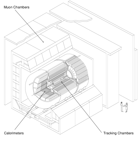
FIG. 1.: Cut away isometric view of the DØ detector.

DØ is a multipurpose detector designed to study $p\overline{p}$ collisions at the Fermilab Tevatron Collider. The detector was commissioned during the summer of 1992. The work presented here is based on approximately $125\ \text{pb}^{-1}$ of accumulated data recorded during the 1992–1996 collider runs. A full description of the detector may be found in Ref. [10]. Here, we describe briefly the properties of the detector that are relevant for the top quark mass measurement.

The detector was designed to have good electron and muon identification capabilities, and to measure jets and missing transverse energy ${\hbox{$E$\kern-6.00006pt\lower-0.43057pt\hbox{/}}}_{T}$ with good resolution. The detector consists of three major systems: a nonmagnetic central tracking system, a hermetic uranium liquid-argon calorimeter, and a muon spectrometer. A cut away view of the detector is shown in Fig. 1.

The central detector (CD) consists of four tracking subsystems: a vertex drift chamber, a transition radiation detector (not used for this analysis), a central drift chamber, and two forward drift chambers. It measures the trajectories of charged particles and can discriminate between single charged particles and $e^{+}e^{-}$ pairs from photon conversions by measuring the ionization along their tracks. It covers the region $|\eta|<3.2$ in pseudorapidity, where $\eta=\tanh^{-1}(\cos\theta)$. (We define $\theta$ and $\phi$ to be the polar and azimuthal angles, respectively.)

The calorimeter is divided into three parts: the central calorimeter (CC) and the two end calorimeters (EC), which together cover the pseudorapidity range $|\eta|<4.2$. The inner electromagnetic (EM) portion of the calorimeters is 21 radiation lengths deep, and is divided into four longitudinal segments (layers). The outer hadronic portions are 7–9 nuclear interaction lengths deep, and are divided into four (CC) or five (EC) layers. The calorimeters are transversely segmented into pseudoprojective towers with $\Delta\eta\times\Delta\phi$ = $0.1\times 0.1$. The third layer of the electromagnetic (EM) calorimeter, in which the maximum of EM showers is expected, is segmented twice as finely in both $\eta$ and $\phi$, with cells of size $\Delta\eta\times\Delta\phi$ = $0.05\times 0.05$.

Since muons from top quark decays populate predominantly the central region, this work uses only the central portion of the DØ muon system, covering $|\eta|<1.7$. This system consists of four planes of proportional drift tubes in front of magnetized iron toroids with a magnetic field of 1.9 T and two groups of three planes each of proportional drift tubes behind the toroids. The magnetic field lines and the wires in the drift tubes are oriented transversely to the beam direction. The muon momentum $p^{\mu}$ is measured from the muon’s deflection angle in the magnetic field of the toroid.

A separate synchrotron, the Main Ring, lies above the Tevatron and passes through the outer region of the DØ calorimeter. During data-taking, it is used to accelerate protons for antiproton production. Losses from the Main Ring may deposit energy in the calorimeters, increasing the instrumental background. We reject much of this background at the trigger level by not accepting triggers during injection into the Main Ring, when losses are large. Some triggers are also disabled whenever a Main Ring bunch passes through the detector or when losses are registered in scintillation counters around the Main Ring.

III Event Selection

For the purposes of this analysis, we divide the lepton + jets final states into electron and muon channels. We further subdivide these channels based on whether or not a muon consistent with $b\rightarrow\mu+X$ is present. We thus have four channels, which will be denoted $e+\text{jets}$, $\mu+\text{jets}$, $e+\text{jets}/\mu$, and $\mu+\text{jets}/\mu$.

The event sample used for determining the top quark mass is selected using criteria similar to those used for the $t\overline{t}$ production cross section measurement [8], with the exception of the cuts on the event shape variables $H_{T}\equiv\sum E_{T}^{\text{jet}}$ and aplanarity. The particle identification, trigger requirements, and event selection cuts are summarized below. More detailed information about triggering, particle identification, and jet and ${\hbox{$E$\kern-6.00006pt\lower-0.43057pt\hbox{/}}}_{T}$ reconstruction may be found in Ref. [6]. (Note, however, that the current electron and muon identification algorithms provide better rejection of backgrounds and increased efficiencies than those used in Ref. [6].)

A Particle identification

1 Electrons

Electron identification is based on a likelihood technique. Candidates are first identified by finding isolated clusters of energy in the EM calorimeter with a matching track in the central detector. We then cut on a likelihood constructed from the following four variables:

• The $\chi^{2}$ from a covariance matrix which measures the consistency of the calorimeter cluster shape with that of an electron shower.

• The electromagnetic energy fraction, defined as the ratio of the portion of the energy of the cluster found in the EM calorimeter to its total energy.

• A measure of the consistency between the track position and the cluster centroid.

• The ionization $dE/dx$ along the track.

To a good approximation, these four variables are independent of each other for electron candidates.

Electrons from $W$ boson decay tend to be isolated, even in $t\overline{t}$ events. Thus, we make the additional cut

$${E_{\text{tot}}(0.4)-E_{\text{EM}}(0.2)\over E_{\text{EM}}(0.2)}<0.1,$$ (1)

where $E_{\text{tot}}(0.4)$ is the energy within $\Delta R<0.4$ of the cluster centroid ($\Delta R=\sqrt{\Delta\eta^{2}+\Delta\phi^{2}}$) and $E_{\text{EM}}(0.2)$ is the energy in the EM calorimeter within $\Delta R<0.2$.

2 Muons

Two types of muon selection are used in this analysis. The first is used to identify isolated muons from $W\rightarrow\mu\nu$ decay. The other is used to tag $b$-jets by identifying “tag” muons consistent with originating from $b\rightarrow\mu+X$ decay.

Besides cuts on the muon track quality, both selections require that:

• The muon pseudorapidity $|\eta^{\mu}|\leq 1.7$.

• The magnetic field integral $>2.0\ \text{T}\cdot\text{m}$ (equivalent to a momentum change of $0.6\ \text{GeV}/c$).

• The energy deposited in the calorimeter along a muon track be at least that expected from a minimum ionizing particle.

For isolated muons, we apply the following additional selection requirements:

• Transverse momentum $p_{T}\geq 20\ \text{GeV}/c$.

• The distance in the $\eta-\phi$ plane between the muon and the closest jet $\Delta R(\mu,j)>0.5$.

For tag muons, we instead require:

• $p_{T}\geq 4\ \text{GeV}/c$.

• $\Delta R(\mu,j)<0.5$.

3 Jets and missing $E_{T}$

Jets are reconstructed in the calorimeter using a fixed-size cone algorithm. We use a cone size of $\Delta R=0.5$.

Neutrinos are not detected directly. Instead, their presence is inferred from missing transverse energy ${\hbox{$E$\kern-6.00006pt\lower-0.43057pt\hbox{/}}}_{T}$. Two different definitions of ${\hbox{$E$\kern-6.00006pt\lower-0.43057pt\hbox{/}}}_{T}$ are used in the event selection:

• ${\hbox{$E$\kern-6.00006pt\lower-0.43057pt\hbox{/}}}_{T}^{\text{cal}}$, the calorimeter missing $E_{T}$, obtained from the transverse energy of all calorimeter cells.

• ${\hbox{$E$\kern-6.00006pt\lower-0.43057pt\hbox{/}}}_{T}$, the muon corrected missing $E_{T}$, obtained by subtracting the transverse momenta of identified muons from ${\hbox{$E$\kern-6.00006pt\lower-0.43057pt\hbox{/}}}_{T}^{\text{cal}}$.

B Triggers

The DØ trigger system is responsible for reducing the event rate from the beam crossing rate of 286 kHz to the approximately 3–4 Hz which can be recorded on tape. The first stage of the trigger (level 1) makes fast analog sums of the transverse energies in calorimeter trigger towers. These towers have a size of $\Delta\eta\times\Delta\phi=0.2\times 0.2$ and are segmented longitudinally into electromagnetic and hadronic sections. The level 1 trigger operates on these sums along with patterns of hits in the muon spectrometer. It can make a trigger decision within the space of a single beam crossing (unless a level 1.5 decision is required; see below). After level 1 accepts an event, the complete event is digitized and sent to the level 2 trigger, which consists of a farm of 48 general-purpose processors. Software filters running in these processors make the final trigger decision.

The triggers used are defined in terms of combinations of specific objects (electron, muon, jet, ${\hbox{$E$\kern-6.00006pt\lower-0.43057pt\hbox{/}}}_{T}$) required in the level 1 and level 2 triggers. These elements are summarized below. For more information on the DØ trigger system, see Refs. [6, 10].

To trigger on electrons, level 1 requires that the transverse energy in the EM section of a trigger tower be above a programmed threshold. The level 2 electron algorithm examines the regions around the level 1 towers which are above threshold, and uses the full segmentation of the EM calorimeter to identify showers with shapes consistent with those of electrons. The level 2 algorithm can also apply an isolation requirement or demand that there be an associated track in the central detector.

For the latter portion of the run, a “level 1.5” processor was also available for electron triggering. The $E_{T}$ of each EM trigger tower above the level 1 threshold is summed with the neighboring tower with the most energy. A cut is then made on this sum. The hadronic portions of the two towers are also summed, and the ratio of EM transverse energy to total transverse energy in the two towers is required to be above 0.85. The use of a level 1.5 electron trigger is indicated in the tables below as an “EX” tower.

The level 1 muon trigger uses the pattern of drift tubes with hits to provide the number of muon candidates in different regions of the muon spectrometer. A level 1.5 processor may optionally be used to put a $p_{T}$ requirement on the candidates (at the expense of slightly increased dead time). In level 2, the full digitized data are available, and the first stage of the full event reconstruction is performed. The level 2 muon algorithm can optionally require the presence of an energy deposit in the calorimeter consistent with that from a muon; this is indicated in the tables below by “cal confirm”.

For a jet trigger, level 1 requires that the sum of the transverse energies in the EM and hadronic sections of a trigger tower be above a programmed threshold. Alternatively, level 1 can sum the transverse energies within “large tiles” of size $0.8\times 1.6$ in $\eta\times\phi$ and cut on these sums. Level 2 then sums calorimeter cells around the identified towers (or around the $E_{T}$-weighted centroids of the large tiles) in cones of a specified radius $\Delta R$, and imposes a cut on the total transverse energy.

The ${\hbox{$E$\kern-6.00006pt\lower-0.43057pt\hbox{/}}}_{T}$ in the calorimeter can also be computed in both level 1 and level 2. The $z$ position used for the interaction vertex in level 2 is determined from the relative timing of hits in scintillation counters located in front of each EC (level 0).

The trigger requirements used for this analysis are summarized in Tables I–III. These tables are divided according to the three major running periods. Run 1a was from 1992–1993, run 1b was from 1994–1995, and run 1c was during the winter of 1995–1996. Note that not all the triggers listed were active simultaneously, and that differing requirements were used to veto possible Main Ring events. In addition, some of the triggers were prescaled at high luminosity. The “exposure” column in the tables takes these factors into account.

TABLE I.: Triggers used during run 1a (1992–1993). “Exposure” gives the effective integrated luminosity for each trigger, taking into account any prescaling.

Name	$Exposure$	Level 1	Level 2	Used by
	$(\ \text{pb}^{-1})$
ele-high	$11.0$	1 EM tower, $E_{T}>10\ \text{GeV}$	1 isolated $e$, $E_{T}>20\ \text{GeV}$	$e+\text{jets}$
				$e+\text{jets}/\mu$
ele-jet	$14.4$	1 EM tower, $E_{T}>10\ \text{GeV}$, $|\eta|<2.6$	1 $e$, $E_{T}>15\ \text{GeV}$, $|\eta|<2.5$	$e+\text{jets}$
		2 jet towers, $E_{T}>5\ \text{GeV}$	2 jets ($\Delta R=0.3$), $E_{T}>10\ \text{GeV}$, $|\eta|<2.5$	$e+\text{jets}/\mu$
			$\mbox{${\hbox{$E$\kern-6.00006pt\lower-0.43057pt\hbox{/}}}_{T}^{\text{cal}}$}>10\ \text{GeV}$
mu-jet-high	$10.2$	1 $\mu$, $|\eta|<2.4$	1 $\mu$, $p_{T}>8\ \text{GeV}/c$	$\mu+\text{jets}$
		1 jet tower, $E_{T}>5\ \text{GeV}$	1 jet ($\Delta R=0.7$), $E_{T}>15\ \text{GeV}$	$\mu+\text{jets}/\mu$

TABLE II.: Same as Table I for run 1b (1994–1995).

Name	$Exposure$	Level 1	Level 2	Used by
	$(\ \text{pb}^{-1})$
em1-eistrkcc-ms	$93.4$	1 EM tower, $E_{T}>10\ \text{GeV}$	1 isolated $e$ w/track, $E_{T}>20\ \text{GeV}$	$e+\text{jets}$
		1 EX tower, $E_{T}>15$ GeVa	$\mbox{${\hbox{$E$\kern-6.00006pt\lower-0.43057pt\hbox{/}}}_{T}^{\text{cal}}$}>15\ \text{GeV}$	$e+\text{jets}/\mu$
ele-jet-high	$98.0$	1 EM tower, $E_{T}>12\ \text{GeV}$, $|\eta|<2.6$	1 $e$, $E_{T}>15\ \text{GeV}$, $|\eta|<2.5$	$e+\text{jets}$
		2 jet towers, $E_{T}>5\ \text{GeV}$, $|\eta|<2.0$	2 jets ($\Delta R=0.3$), $E_{T}>10\ \text{GeV}$, $|\eta|<2.5$	$e+\text{jets}/\mu$
			$\mbox{${\hbox{$E$\kern-6.00006pt\lower-0.43057pt\hbox{/}}}_{T}^{\text{cal}}$}>14\ \text{GeV}$
mu-jet-high	$66.4$	1 $\mu$, $p_{T}>7\ \text{GeV}/c$a, $|\eta|<1.7$	1 $\mu$, $p_{T}>10\ \text{GeV}/c$, $|\eta|<1.7$	$\mu+\text{jets}$
		1 jet tower, $E_{T}>5\ \text{GeV}$, $|\eta|<2.0$a	1 jet ($\Delta R=0.7$), $E_{T}>15\ \text{GeV}$, $|\eta|<2.5$	$\mu+\text{jets}/\mu$
mu-jet-cal	$88.0$	1 $\mu$, $p_{T}>7\ \text{GeV}/c$a, $|\eta|<1.7$	1 $\mu$, $p_{T}>10\ \text{GeV}/c$, $|\eta|<1.7$, cal confirm	$\mu+\text{jets}$
		1 jet tower, $E_{T}>5\ \text{GeV}$, $|\eta|<2.0$a	1 jet ($\Delta R=0.7$), $E_{T}>15\ \text{GeV}$, $|\eta|<2.5$	$\mu+\text{jets}/\mu$
mu-jet-cent	$48.5$	1 $\mu$, $|\eta|<1.0$	1 $\mu$, $p_{T}>10\ \text{GeV}/c$, $|\eta|<1.0$	$\mu+\text{jets}$
		1 jet tower, $E_{T}>5\ \text{GeV}$, $|\eta|<2.0$	1 jet ($\Delta R=0.7$), $E_{T}>15\ \text{GeV}$, $|\eta|<2.5$	$\mu+\text{jets}/\mu$
mu-jet-cencal	$51.2$	1 $\mu$, $|\eta|<1.0$	1 $\mu$, $p_{T}>10\ \text{GeV}/c$, $|\eta|<1.0$, cal confirm	$\mu+\text{jets}$
		1 jet tower, $E_{T}>5\ \text{GeV}$, $|\eta|<2.0$	1 jet ($\Delta R=0.7$), $E_{T}>15\ \text{GeV}$, $|\eta|<2.5$	$\mu+\text{jets}/\mu$
jet-3-mu	$11.9$	3 jet towers, $E_{T}>5\ \text{GeV}$	3 jets ($\Delta R=0.7$), $E_{T}>15\ \text{GeV}$, $|\eta|<2.5$	$\mu+\text{jets}$
		$\mbox{${\hbox{$E$\kern-6.00006pt\lower-0.43057pt\hbox{/}}}_{T}^{\text{cal}}$}>20\ \text{GeV}$	$\mbox{${\hbox{$E$\kern-6.00006pt\lower-0.43057pt\hbox{/}}}_{T}^{\text{cal}}$}>17\ \text{GeV}$	$\mu+\text{jets}/\mu$
jet-3-miss-low	$57.8$	3 large tiles, $E_{T}>15$, $|\eta|<2.4$	3 jets ($\Delta R=0.5$), $E_{T}>15\ \text{GeV}$, $|\eta|<2.5$	$\mu+\text{jets}$
		3 jet towers, $E_{T}>7\ \text{GeV}$, $|\eta|<2.6$	$\mbox{${\hbox{$E$\kern-6.00006pt\lower-0.43057pt\hbox{/}}}_{T}^{\text{cal}}$}>17\ \text{GeV}$	$\mu+\text{jets}/\mu$
jet-3-l2mu	$25.8$	3 large tiles, $E_{T}>15$, $|\eta|<2.4$	1 $\mu$, $p_{T}>6\ \text{GeV}/c$, $|\eta|<1.7$, cal confirm	$\mu+\text{jets}$
		3 jet towers, $E_{T}>7\ \text{GeV}$, $|\eta|<2.6$	3 jets ($\Delta R=0.5$), $E_{T}>15\ \text{GeV}$, $|\eta|<2.5$	$\mu+\text{jets}/\mu$
			$\mbox{${\hbox{$E$\kern-6.00006pt\lower-0.43057pt\hbox{/}}}_{T}^{\text{cal}}$}>17\ \text{GeV}$

TABLE III.: Same as Table I for run 1c (1995–1996).

Name	$Exposure$	Level 1	Level 2	Used by
	$(\ \text{pb}^{-1})$
ele-jet-high	$1.9$	1 EM tower, $E_{T}>12\ \text{GeV}$, $|\eta|<2.6$	1 $e$, $E_{T}>15\ \text{GeV}$, $|\eta|<2.5$	$e+\text{jets}$
		2 jet towers, $E_{T}>5\ \text{GeV}$, $|\eta|<2.0$	2 jets ($\Delta R=0.3$), $E_{T}>10\ \text{GeV}$, $|\eta|<2.5$	$e+\text{jets}/\mu$
			$\mbox{${\hbox{$E$\kern-6.00006pt\lower-0.43057pt\hbox{/}}}_{T}^{\text{cal}}$}>14\ \text{GeV}$
ele-jet-higha	$11.0$	1 EM tower, $E_{T}>12\ \text{GeV}$, $|\eta|<2.6$	1 $e$, $E_{T}>17\ \text{GeV}$, $|\eta|<2.5$	$e+\text{jets}$
		2 jet towers, $E_{T}>5\ \text{GeV}$, $|\eta|<2.0$	2 jets ($\Delta R=0.3$), $E_{T}>10\ \text{GeV}$, $|\eta|<2.5$	$e+\text{jets}/\mu$
		1 EX tower, $E_{T}>15\ \text{GeV}$	$\mbox{${\hbox{$E$\kern-6.00006pt\lower-0.43057pt\hbox{/}}}_{T}^{\text{cal}}$}>14\ \text{GeV}$
mu-jet-cent	$8.9$	1 $\mu$, $|\eta|<1.0$	1 $\mu$, $p_{T}>12\ \text{GeV}/c$, $|\eta|<1.0$	$\mu+\text{jets}$
		1 jet tower, $E_{T}>5\ \text{GeV}$, $|\eta|<2.0$	1 jet ($\Delta R=0.7$), $E_{T}>15\ \text{GeV}$, $|\eta|<2.5$	$\mu+\text{jets}/\mu$
		2 jet towers, $E_{T}>3\ \text{GeV}$
mu-jet-cencal	$11.4$	1 $\mu$, $|\eta|<1.0$	1 $\mu$, $p_{T}>12\ \text{GeV}/c$, $|\eta|<1.0$, cal confirm	$\mu+\text{jets}$
		1 jet tower, $E_{T}>5\ \text{GeV}$, $|\eta|<2.0$	1 jet ($\Delta R=0.7$), $E_{T}>15\ \text{GeV}$, $|\eta|<2.5$	$\mu+\text{jets}/\mu$
		2 jet towers, $E_{T}>3\ \text{GeV}$
jet-3-l2mu	$11.3$	3 large tiles, $E_{T}>15$, $|\eta|<2.4$	1 $\mu$, $p_{T}>8\ \text{GeV}/c$, $|\eta|<1.7$, cal confirm	$\mu+\text{jets}$
		3 jet towers, $E_{T}>5\ \text{GeV}$, $|\eta|<2.0$	3 jets ($\Delta R=0.5$), $E_{T}>15\ \text{GeV}$, $|\eta|<2.5$	$\mu+\text{jets}/\mu$
		4 jet towers, $E_{T}>3\ \text{GeV}$	$\mbox{${\hbox{$E$\kern-6.00006pt\lower-0.43057pt\hbox{/}}}_{T}^{\text{cal}}$}>17\ \text{GeV}$

C Event selection

The first set of cuts used to define the sample for mass analysis is very similar to that used for the cross section analysis [8]:

• An isolated electron or muon with $E_{T}>20\ \text{GeV}$.

• $|\eta^{e}|<2.0$ or $|\eta^{\mu}|<1.7$.

• At least 4 jets with $E_{T}>15\ \text{GeV}$ and $|\eta^{\text{jet}}|<2.0$.

• $\mbox{${\hbox{$E$\kern-6.00006pt\lower-0.43057pt\hbox{/}}}_{T}^{\text{cal}}$}>25\ \text{GeV}$ for $e$+jets (untagged) or $\mbox{${\hbox{$E$\kern-6.00006pt\lower-0.43057pt\hbox{/}}}_{T}^{\text{cal}}$}>20\ \text{GeV}$ for $\mu$+jets (both tagged and untagged).

• $\mbox{${\hbox{$E$\kern-6.00006pt\lower-0.43057pt\hbox{/}}}_{T}$}>20\ \text{GeV}$.

We reject events which contain photons — isolated clusters in the EM calorimeter with shapes consistent with an EM shower and with a poor match to any track in the central detector, and satisfying $E_{T}>15\ \text{GeV}$ and $|\eta|<2$. Three such events are rejected. We also reject events which contain extra isolated high-$p_{T}$ electrons or which fail additional cuts to remove calorimeter noise and Main Ring effects.

After these cuts, the remaining background is primarily $W+\text{jets}$, with a small ($\approx 20\%$) admixture of QCD multijet events in which a jet is misidentified as a lepton.

If a candidate has a tag muon, we require it to pass additional cuts on the direction of the ${\hbox{$E$\kern-6.00006pt\lower-0.43057pt\hbox{/}}}_{T}$ vector. For the $e+\text{jets}/\mu$ channel, we require

• $\mbox{${\hbox{$E$\kern-6.00006pt\lower-0.43057pt\hbox{/}}}_{T}$}>35\ \text{GeV}$, if $\Delta\phi(\mbox{${\hbox{$E$\kern-6.00006pt\lower-0.43057pt\hbox{/}}}_{T}$},\mu)<25^{\circ}$,

while for the $\mu+\text{jets}/\mu$ channel, we require that the highest-$p_{T}$ muon satisfy

• $\Delta\phi(\mbox{${\hbox{$E$\kern-6.00006pt\lower-0.43057pt\hbox{/}}}_{T}$},\mu)<170^{\circ}$ and

• $|\Delta\phi(\mbox{${\hbox{$E$\kern-6.00006pt\lower-0.43057pt\hbox{/}}}_{T}$},\mu)-90^{\circ}|/90^{\circ}<\mbox{${\hbox{$E$\kern-6.00006pt\lower-0.43057pt\hbox{/}}}_{T}$}/(45\ \text{GeV})$.

These cuts remove QCD multijet background events which appear to have a large ${\hbox{$E$\kern-6.00006pt\lower-0.43057pt\hbox{/}}}_{T}$ due to a mismeasurement of the muon momentum.

For the remaining, untagged, events, we require:

• $E_{T}^{W}\equiv|E_{T}^{\text{lep}}|+|\mbox{${\hbox{$E$\kern-6.00006pt\lower-0.43057pt\hbox{/}}}_{T}$}|>60\ \text{GeV}$.

• $|\eta^{W}|<2.0$.

For the purpose of these two cuts, we define $\eta^{W}$ by assuming that the entire ${\hbox{$E$\kern-6.00006pt\lower-0.43057pt\hbox{/}}}_{T}$ of the event is due to the neutrino from the decay of the $W$ boson. The longitudinal component of the neutrino momentum $p_{z}^{\nu}$ is found by using the $W$ boson mass $M_{W}$ as a constraint. If the transverse mass of the lepton and neutrino $M_{T}(l\nu)$ is less than $M_{W}$, there are two real solutions; the one with the smallest absolute value of $p_{z}^{\nu}$ is used. Monte Carlo studies show that this is the correct solution about $80\%$ of the time. If $M_{T}(l\nu)>M_{W}$ there are no real solutions. In this case, the ${\hbox{$E$\kern-6.00006pt\lower-0.43057pt\hbox{/}}}_{T}$ is scaled so that $M_{T}(l\nu)=M_{W}$. This scaled ${\hbox{$E$\kern-6.00006pt\lower-0.43057pt\hbox{/}}}_{T}$ is also used for the $E_{T}^{W}$ cut (but not for the previous cuts on ${\hbox{$E$\kern-6.00006pt\lower-0.43057pt\hbox{/}}}_{T}$ alone).

This cut on $E_{T}^{W}$ removes a portion of the QCD multijet background. Figure 2 compares the $E_{T}^{W}$ distribution for this background to that from Monte Carlo $W+\text{jets}$ events.

We show in Fig. 3 the distributions of $|\eta^{W}|$ for our data and for the Monte Carlo prediction. The data are seen to significantly exceed the prediction of the vecbos Monte Carlo (described in Sec. V) in the far forward region. The amount of $t\overline{t}$ signal with $|\eta^{W}|>2$ is only a few percent ($\approx 3\%$ for $m_{t}=175\ \text{GeV}/c^{2}$). In addition, a check of the $W$ boson transverse mass and ${\hbox{$E$\kern-6.00006pt\lower-0.43057pt\hbox{/}}}_{T}$ distributions shows that the QCD multijet background plays no unusually prominent role at high $|\eta^{W}|$. We note that the vecbos Monte Carlo, while the best currently available, is only a tree-level calculation of the $W+\text{jets}$ process. Particularly in the forward direction, one would expect higher order corrections to play a larger role. To mitigate the effects of this discrepancy, and to further reduce the background, we require $|\eta^{W}|<2$. Once this cut is made, the $\chi^{2}_{L}$ between the data and prediction is 12.2 for 7 d.o.f., giving a $9\%$ probability. ($\chi^{2}_{L}\equiv 2\sum_{i}\left[y_{i}-N_{i}+N_{i}\ln(N_{i}/y_{i})\right]$, where $N$ is the number of observed events and $y$ is the total number expected from Monte Carlo. This form is appropriate for low statistics [11].) The contribution of this effect to the systematic error will be discussed in Sec. VII G 2 (and is found to be negligible).

These event selection cuts are summarized in Table IV. When applied to the approximately $125\ \text{pb}^{-1}$ of data from the 1992–1996 collider runs, 91 events are selected [12], seven of which have a tag muon. This sample will be referred to as the “precut” sample, and the set of cuts as the “PR” cuts. One additional cut is made to define the final sample. This is based on the $\chi^{2}$ of a kinematic fit to the $t\overline{t}$ decay hypothesis ($\chi^{2}<10$), and is described in Sec. VII. This final cut reduces the sample to 77 candidate events, of which five are tagged.

TABLE IV.: Summary of event selection cuts.

Channel	$e+\text{jets}$	$\mu+\text{jets}$	$e+\text{jets}/\mu$	$\mu+\text{jets}/\mu$
Lepton	$E_{T}^{e}>20\ \text{GeV}$	$p_{T}^{\mu}>20\ \text{GeV}/c$	$E_{T}^{e}>20\ \text{GeV}$	$p_{T}^{\mu}>20\ \text{GeV}/c$
	$|\eta^{e}|<2$	$|\eta^{\mu}|<1.7$	$|\eta^{e}|<2$	$|\eta^{\mu}|<1.7$
${\hbox{$E$\kern-6.00006pt\lower-0.43057pt\hbox{/}}}_{T}$	$\mbox{${\hbox{$E$\kern-6.00006pt\lower-0.43057pt\hbox{/}}}_{T}$}>20\ \text{GeV}$	$\mbox{${\hbox{$E$\kern-6.00006pt\lower-0.43057pt\hbox{/}}}_{T}$}>20\ \text{GeV}$	$\mbox{${\hbox{$E$\kern-6.00006pt\lower-0.43057pt\hbox{/}}}_{T}$}>20\ \text{GeV}$	$\mbox{${\hbox{$E$\kern-6.00006pt\lower-0.43057pt\hbox{/}}}_{T}$}>20\ \text{GeV}$
	$\mbox{${\hbox{$E$\kern-6.00006pt\lower-0.43057pt\hbox{/}}}_{T}^{\text{cal}}$}>25\ \text{GeV}$	$\mbox{${\hbox{$E$\kern-6.00006pt\lower-0.43057pt\hbox{/}}}_{T}^{\text{cal}}$}>20\ \text{GeV}$		$\mbox{${\hbox{$E$\kern-6.00006pt\lower-0.43057pt\hbox{/}}}_{T}^{\text{cal}}$}>20\ \text{GeV}$
Jets	$\geq 4\ \text{jets}$	$\geq 4\ \text{jets}$	$\geq 4\ \text{jets}$	$\geq 4\ \text{jets}$
	$E_{T}^{\text{jet}}>15\ \text{GeV}$	$E_{T}^{\text{jet}}>15\ \text{GeV}$	$E_{T}^{\text{jet}}>15\ \text{GeV}$	$E_{T}^{\text{jet}}>15\ \text{GeV}$
	$|\eta^{\text{jet}}|<2.0$	$|\eta^{\text{jet}}|<2.0$	$|\eta^{\text{jet}}|<2.0$	$|\eta^{\text{jet}}|<2.0$
$\mu$ Tag	No tag	No tag	Tag required	Tag required
Other	$E_{T}^{W}>60\ \text{GeV}$	$E_{T}^{W}>60\ \text{GeV}$	$\mbox{${\hbox{$E$\kern-6.00006pt\lower-0.43057pt\hbox{/}}}_{T}$}>35\ \text{GeV}$	$\Delta\phi(\mbox{${\hbox{$E$\kern-6.00006pt\lower-0.43057pt\hbox{/}}}_{T}$},\mu)<170^{\circ}$
	$|\eta^{W}|<2.0$	$|\eta^{W}|<2.0$	if $\Delta\phi(\mbox{${\hbox{$E$\kern-6.00006pt\lower-0.43057pt\hbox{/}}}_{T}$},\mu)<25^{\circ}$	$|\Delta\phi(\mbox{${\hbox{$E$\kern-6.00006pt\lower-0.43057pt\hbox{/}}}_{T}$},\mu)-90^{\circ}|/90^{\circ}<$
				$\mbox{${\hbox{$E$\kern-6.00006pt\lower-0.43057pt\hbox{/}}}_{T}$}/(45\ \text{GeV})$
Events passing cuts	43	41	4	3
With $\chi^{2}<10$	35	37	2	3

FIG. 2.: $E_{T}^{W}$ distribution for Monte Carlo $W$+jets events (solid histogram) and for QCD multijet background data (dashed histogram). All selection cuts are applied except for the $E_{T}^{W}$ cut. The arrow shows the cut value. (The normalizations are taken from the result of the LB fit to the data, as described in Sec. VII E, with channels combined as described in Sec. VII D. The models used to simulate the data are described in Sec. V.)

FIG. 3.: $|\eta^{W}|$ distribution for data (histogram), predicted signal plus background (filled circles), and background alone (open triangles). All selection cuts are applied except for the $\eta^{W}$ cut. The arrow shows the cut value. (The normalizations are as in Fig. 2.)

IV Jet Corrections and Energy Scale Error

To calibrate the energy scale so that data and Monte Carlo (MC) are on an equal footing, we apply a series of energy corrections to the measured objects. These corrections are carried out in three steps. The first of these corrections is done before events are selected and is used by most DØ analyses; the other two corrections are applied during the kinematic fit and are specific to the top quark mass analysis.

A Standard corrections

For the standard corrections, electromagnetic objects are first scaled by a factor which was chosen to make the invariant mass peak from dielectron events match the $Z$ boson mass as measured by the LEP experiments. (This factor is determined separately for each of the three cryostats of the calorimeter.) Next, jet energies are corrected using

$$E(\text{corrected})={E(\text{measured})-O\over R(1-S)}.$$ (2)

Here, $R$ is the calorimeter response; it is found using $E_{T}$ balance (as determined from the total ${\hbox{$E$\kern-6.00006pt\lower-0.43057pt\hbox{/}}}_{T}$) in $\gamma+\text{jets}$ events. This determination is done separately and symmetrically for both data and Monte Carlo. $O$ is the offset due to the underlying event, multiple interactions, and noise from the natural radioactivity of the uranium absorber. It is determined by comparing data in which a hard interaction is required to data in which that requirement is relaxed, and by comparing data taken at different luminosities. The term $S$ is the fractional shower leakage outside the jet cone in the calorimeter. It is determined by using single particle showers measured in the test beam to construct simulated showers from MC jets; this leakage is approximately $3\%$ for a $50\ \text{GeV}$ jet ($\Delta R=0.5$) in the central calorimeter. Further details about these corrections may be found in Ref. [13].

B Parton-level corrections

The procedure of the previous section corrects for the portions of showers in the calorimeter which spread outside of the jet cone, but not for any radiation outside of the cone. Thus, the corrected jet energies are systematically lower than the corresponding parton-level energies (i.e., before QCD evolution or fragmentation in the MC). We make a correction to match the scale of the jet energies to that of the unfragmented partons in the MC.

FIG. 4.: The measured jet energies for quarks from $W\rightarrow q\overline{q}$ in $t\overline{t}$ MC are plotted against the corresponding parton energies. Radiation outside of the jet cone causes the measured jet energy to be lower than the energy at the parton level. The dashed line is drawn along the diagonal, and the solid line is a linear fit to the points. This plot is based on herwig fragmentation with $|\eta_{\text{det}}^{\text{jet}}|<0.2$.

To derive this correction, we use herwig [14] $t\overline{t}$ Monte Carlo and match reconstructed jets to the partons from top quark decay. Their energies are then plotted against each other, as in Fig. 4. This relation is observed to be nearly linear. We fit it separately for light quark jets and for untagged $b$ quark jets. The results are given in Table V for different regions in $\eta_{\text{det}}$ ($\eta_{\text{det}}$ $\equiv$ ‘detector-$\eta$’ $\equiv$ the pseudorapidity corresponding to a particle coming from the geometric center of the detector, rather than from the interaction vertex). Separating the $b$ quark jets allows us to correct, on average, for the neutrinos from $b$ decays. This correction is observed not to depend strongly on the MC top quark mass.

TABLE V.: Parameters for parton-level jet corrections. $E(\text{corrected})=(E-A)/B$.

	Light quark jets		Untagged $b$ jets
$\eta$ region	$A(\text{GeV})$	$B$	$A(\text{GeV})$	$B$
$0.0<|\eta_{\text{det}}|<0.2$	$0.322$	$0.933$	$-0.672$	$0.907$
$0.2<|\eta_{\text{det}}|<0.6$	$0.635$	$0.930$	$-1.34$	$0.914$
$0.6<|\eta_{\text{det}}|<0.9$	$1.86$	$0.883$	$0.002$	$0.868$
$0.9<|\eta_{\text{det}}|<1.3$	$1.70$	$0.933$	$-0.548$	$0.904$
$1.3<|\eta_{\text{det}}|$	$4.50$	$0.882$	$2.46$	$0.859$

For tagged $b$ quark jets, we have additional information from the tag muon. However, the momentum spectrum of muons from $b$ quark decay in $t\overline{t}$ events is rather steeply falling; furthermore, the resolution of the muon system is more nearly Gaussian in the inverse momentum $1/p$ than in $p$. Thus, measurement errors will cause the measured momentum of a tag muon to be biased upwards. We correct for this bias using $t\overline{t}$ MC, as illustrated in Fig. 5. We then further scale the muon momentum to account for the unobserved neutrino, as shown in Fig. 6. The jet itself is corrected using the light quark corrections; the estimated leptonic energy is then added to this corrected jet energy.

FIG. 5.: Correlation between the measured momentum and the true momentum of the tag muon in Monte Carlo $t\overline{t}$ events. The curve is the result of an empirical fit, $47.19[1-\exp(-0.03398-0.01593p^{\mu}-0.0005554(p^{\mu})^{2})]$.

FIG. 6.: Correlation between the tag muon momentum and the total leptonic energy from $b$ quark decay in MC $t\overline{t}$ events. The curve is the result of an empirical fit, $1.313+\exp(3.101-0.6528p^{\mu})+\exp(0.4622-0.06514p^{\mu})$.

C $\eta$-dependent adjustment and energy scale error

For the final corrections, we study the response of the detector to $\gamma+1\ \text{jet}$ events, using both data and Monte Carlo. We select events containing exactly one photon with $E_{T}^{\gamma}>20\ \text{GeV}$, $|\eta_{\text{det}}^{\gamma}|<1.0$ or $1.6<|\eta_{\text{det}}^{\gamma}|<2.5$, and exactly one reconstructed jet of any energy (excluding the photon). We require that the jet satisfy $E_{T}>15\ \text{GeV}$, $|\eta|<2$, and $|\pi-\Delta\phi(j,\gamma)|<0.2\ \text{rad}$. We reject events with Main Ring activity and those which are likely to be multiple interactions. To reject $W$ boson decays, we further require that $\mbox{${\hbox{$E$\kern-6.00006pt\lower-0.43057pt\hbox{/}}}_{T}$}/E_{T}^{\gamma}<1.2$ if $E_{T}^{\gamma}<25\ \text{GeV}$, or $\mbox{${\hbox{$E$\kern-6.00006pt\lower-0.43057pt\hbox{/}}}_{T}$}/E_{T}^{\gamma}<0.65$ otherwise. With this selection, we compute

$$\Delta S=\left\langle E_{T}^{\text{jet}}-E_{T}^{\gamma}\over E_{T}^{\gamma}\right\rangle$$ (3)

and plot it as a function of $\eta_{\text{det}}^{\text{jet}}$. The result is shown in Fig. 7. This reveals detector inhomogeneities in the transition region between the central and end calorimeters [15]. The curve from Monte Carlo is also seen to have a somewhat different shape than that from data. To remove these effects, we smooth the $\Delta S$ distributions by fitting them to the sum of several Gaussians, and scale each jet by $1/(1+\Delta S(\eta_{\text{det}}^{\text{jet}}))$. This is done separately for data and for Monte Carlo.

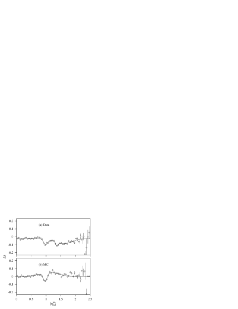
FIG. 7.: The energy scale deviation $\Delta S$ as a function of $\eta_{\text{det}}^{\text{jet}}$ for (a) data and (b) Monte Carlo. The curves are empirical multigaussian fits to the points.

To estimate the uncertainty in the relative scale between data and Monte Carlo after all corrections, we derive $\Delta S$ as a function of $E_{T}^{\gamma}$ (averaging over $\eta_{\text{det}}^{\text{jet}}$) for both data and MC after all corrections have been applied. The difference of the two is plotted in Fig. 8, along with a band of $\pm(2.5\%+0.5\ \text{GeV})$, which we use as our estimate of the systematic error of the jet energy calibration. (It is the relative data-MC difference that is relevant, rather than the absolute error, since the final mass is extracted by comparing the data to MC generated with known top quark masses.)

FIG. 8.: The relative energy scale difference between data and MC as a function of photon $E_{T}$ after all jet corrections are applied. The curves are the error band $\pm(2.5\%+{0.5\ \text{GeV}})$.

A cross-check of these corrections is provided by $(Z\rightarrow ee)+\text{jets}$ events. As shown in Fig. 9, the corrected jets satisfactorily balance the $Z$ boson. We also show in Fig. 10 the $W\rightarrow q\overline{q}$ and $t\rightarrow bq\overline{q}$ masses from $t\overline{t}$ MC before and after the final two corrections. It is seen that the proper masses are recovered.

The accuracy of these corrections depends on how well the Monte Carlo models jet widths. Studies of jets in DØ data show that herwig models the transverse energy distribution within jets to within 5–$10\%$ [16]. Note, however, that since the determination of the response is done separately for data and for Monte Carlo, any disagreements would, to first order, be removed from the energy scale determination. There can still be second-order effects: for example, if jets in herwig were slightly too narrow, and if two jets were to overlap slightly, then the perturbation to the apparent jet energies due to that overlap would be slightly underestimated in the Monte Carlo. For this situation, we calculate that the fraction of the energy of a jet between $R=0.5$ and $R=1.0$ of the jet axis which leaks into the nearest jet is about $10\%$. We further find that this region in $R$ contains about $10\%$ of the total energy of a herwig jet. Thus, the leakage of energy from a jet to a neighbor is on the order of $1\%$. If the fraction of the jet energy outside of $R=0.5$ is substantially larger in data than in herwig, e.g., $20\%$, a $1\%$ miscalibration would result. This is well within the errors we assign for moderate $E_{T}$ jets.

FIG. 9.: Transverse energy balance for $(Z\rightarrow ee)+\text{jets}$ events. The vector $\vec{p}_{T}^{\,Z}+\sum_{\text{jets}}\vec{E}_{T}^{\text{jet}}$ is projected onto the angle bisector of the two electrons. All jet corrections are applied. The curve is a Gaussian fit to the histogram.

FIG. 10.: Masses of $W\rightarrow q\overline{q}$ and $t\rightarrow bq\overline{q}$ in $t\overline{t}$ MC with $m_{t}=175\ \text{GeV}/c^{2}$, both (a), (b) with standard corrections only and (c), (d) with all jet corrections. The arrows locate the input $W$ boson and top quark masses.

V Event Simulation

Monte Carlo simulation is used to model the final states expected from top quark decays and their principal physics backgrounds. Although the overall background normalization is estimated using the observed data, the simulation is essential to determine the expected shapes of kinematic distributions.

A Signal events

Our primary model for $t\overline{t}$ production is the herwig generator, version 5.7, with CTEQ3M [17] parton distribution functions. herwig models $t\overline{t}$ production starting with the elementary hard process, choosing the parton momenta according to matrix element calculations. Initial and final state gluon emission is modeled using leading log QCD evolution [18]. Each top quark is then decayed to a $W$ boson and a $b$ quark, and final state partons are hadronized into jets. Underlying spectator interactions are also included in the model.

For this analysis, samples are generated with top quark masses between 110 and $230\ \text{GeV}/c^{2}$. To increase the efficiency in the processing of lepton plus jets events, one of the $W$ bosons is forced to decay to one of the three lepton families. Events with no final state electrons or muons are vetoed, and half of the events in which both $W$ bosons decayed leptonically are discarded in order to preserve the proper branching ratios. The generated events are run through the døgeant detector simulation [19, 20] and the DØ event reconstruction program.

Additional samples are made using the isajet [21] generator to allow for cross-checks.

B W+jets background

The background due to the production of a $W$ boson along with multiple jets is modeled using the vecbos [22] event generator. vecbos supplies final state partons as a result of a leading order calculation which incorporates the exact tree level matrix elements for $W$ and $Z$ boson production with up to four additional partons. To include the effects of additional radiation and the underlying processes, and to model the hadronization of final state partons, the output of vecbos is passed through herwig’s QCD evolution and fragmentation stages. Since herwig requires information about the color labels of its input partons, it and vecbos were modified to assign color and flavor to the generated partons. Flavors are assigned probabilistically by keeping track of the relative weights of each diagram contributing to the process. Color labels are simply assigned randomly. To estimate systematic errors, we also generate samples which use isajet instead of herwig to fragment the vecbos partons. We test the reliability of the herwig and isajet simulations of higher order processes by comparing $W+$ four jet events generated using the vecbos $W+$ four jet process to those generated using the $W+$ three jet process.

Events are generated using the same parton distribution functions assumed for the signal sample. The dynamical scale of the process is set to be the average jet $p_{T}$. Systematic uncertainties arising from this choice are estimated by changing the scale to the mass of the $W$ boson in a second sample of events. The background samples are processed through the detector simulation, reconstruction, and event selection in the same manner as for the signal samples.

C QCD multijet background

The non-$W$ QCD multijet background is estimated, both for the electron and the muon channels, using background-enriched data samples. In the former channels, the sample consists of events containing highly electromagnetic jets failing the electron identification cuts. In the latter, events are selected containing a muon which fails the isolation requirement, but which otherwise passes the muon identification cuts.

VI Top Discriminants

The key feature that distinguishes top quark events from the $W$+jets and QCD multijet backgrounds is the fitted mass $m_{\text{fit}}$ obtained from kinematic fits of the events to the top quark decay hypothesis. Since the top quark is heavy, the fitted mass tends to be larger for top quark events than for the backgrounds. Therefore, if both the signal to background ratio and the signal are large enough, we should see a clear signal peak in the $m_{\text{fit}}$ distribution. However, there is a caveat: this is true only if the cuts to enhance the signal to noise ratio do not significantly distort the fitted mass distributions. Unfortunately, powerful selection variables such as $H_{T}\equiv\sum E_{T}^{\text{jet}}$ tend to be highly correlated with the fitted mass. Cuts on them thus introduce severe distortions in $m_{\text{fit}}$ which reduce the differences between the distributions for $t\overline{t}$ signal and background, and between the distributions for $t\overline{t}$ signal at different top quark masses, thus impairing the mass measurement.

This distortion of the $m_{\text{fit}}$ distribution can be avoided by using variables which are only weakly correlated with the fitted mass. The challenge is to find variables that also provide a useful measure of discrimination between signal and background. After an extensive search of variables that exploit the expected qualitative differences between the kinematics of top quark events and the backgrounds, we have succeeded in finding four variables $x_{1}$–$x_{4}$ with the desired properties.

This success, however, comes at a price: the discrimination afforded by these variables tends to be weaker than that provided by variables, like $H_{T}$, that are mass dependent. But by treating these variables collectively, rather than applying a cut on each separately, we can compensate for their weaker discrimination. It is most effective to combine the variables into a multivariate discriminant ${\cal D}({\bf x})$ with the general form

$${\cal D}({\bf x})\equiv\frac{f_{s}({\bf x})}{f_{s}({\bf x})+f_{b}({\bf x})},$$ (4)

where ${\bf x}$ denotes the 4-tuple of mass-insensitive variables and $f_{s}({\bf x})$ and $f_{b}({\bf x})$ are functions that pertain to the signal and background, respectively. We choose the functions $f_{s}$ and $f_{b}$ so that ${\cal D}({\bf x})$ is concentrated near zero for the background and near unity for the signal.

In the following sections we describe the variables $x_{1}$–$x_{4}$ and the two complementary forms we have used for the functions $f_{s}({\bf x})$ and $f_{b}({\bf x})$.

A Variables

The four variables $\{x_{1},x_{2},x_{3},x_{4}\}\equiv{\bf x}$ are defined as follows:

$$x_{1} \equiv {\hbox{$E$\kern-6.00006pt\lower-0.43057pt\hbox{/}}}_{T}$$ (5)

$$x_{2} \equiv {\cal{A}}$$ (6)

$$x_{3} \equiv H_{T2}/H_{z}$$ (7)

$$x_{4} \equiv \Delta R^{\text{min}}_{jj}E_{T}^{\text{min}}/E_{T}^{W}.$$ (8)

Our use of the variable $x_{1}$ is motivated by the fact that top quark events have substantial missing transverse energy, due to the neutrino from the leptonically-decaying $W$ boson, while QCD multijet background events do not. Variable $x_{2}$ is the aplanarity ${\cal{A}}$ [23], which is defined in terms of the normalized momentum tensor of the jets and the $W$ boson:

$$M_{ab}=\sum_{i}p_{ia}p_{ib}/\sum_{i}p_{i}^{2},$$ (9)

where $\vec{p}_{i}$ is the three-momentum of the $i$th object in the laboratory frame, and $a,b$ run over $x$, $y$, and $z$. (For this and the remaining two variables, we use all jets satisfying $E_{T}^{\text{jet}}>15\ \text{GeV}$ and $|\eta^{\text{jet}}|<2$.) The $W$ boson momentum is defined by the sum of the lepton and neutrino momentum vectors, where the $z$-component of the neutrino momentum is determined as described in Sec. III C. If the three eigenvalues of $M_{ab}$ are denoted $Q_{j}$ such that

$$Q_{1}\leq Q_{2}\leq Q_{3},$$ (10)

then

$${\cal{A}}={3\over 2}Q_{1}.$$ (11)

This variable is a measure of the degree to which the final state particles lie out of a plane. In $W+\text{jets}$ events, a high $p_{T}$ $W$ boson recoils against a hadronic system that is typically dominated by a single high $p_{T}$ jet. In QCD multijet events, two jets, perturbed by gluon radiation, recoil against each other. The signal, by contrast, has a momentum flow that is more spherical. It therefore has a larger aplanarity than do the backgrounds, which have more longitudinal topologies. (The aplanarity for top quark events is expected to decrease with increasing $m_{t}$ due to the $W$ boson decay products becoming more collimated. This effect, however, is very small for $m_{t}<200\ \text{GeV}/c^{2}$.)

The variable $H_{T}$, as noted above, is a powerful discriminant between signal and background. But, since both the signal and background tend to have at least one high $p_{T}$ jet, we can improve the discrimination somewhat by removing the highest $p_{T}$ jet from $H_{T}$, yielding $H_{T2}$. A plot of this variable is shown in Fig. 11. This variable, however, is correlated with the fitted mass. Therefore, we divide by another mass-sensitive variable, namely $H_{z}$ (equal to the sum of $|p_{z}|$ of the lepton, neutrino, and the jets), in order to reduce that correlation. The longitudinal component of the neutrino momentum is found by the same method used to define $\eta^{W}$. We thus arrive at variable $x_{3}$, which measures the centrality of the events — top quark events being more central than the backgrounds.

FIG. 11.: Plot of $H_{T2}$ for the 77-event candidate sample, compared with the expectation for $m_{t}=175\ \text{GeV}/c^{2}$ signal plus background (filled circles), signal alone (open squares), and background alone (open triangles). (The normalizations are as in Fig. 2.)

The last variable, $x_{4}$, is motivated by the observation that the four highest $E_{T}$ jets in top quark events have a different origin than the jets in $W$+jets and QCD multijet events. For $t\overline{t}$ events, the four highest $E_{T}$ jets are mostly from the decay of the $t\overline{t}$ system. These jets tend to be widely separated in $\eta-\phi$ space. For the backgrounds, usually at least one jet is the result of gluon radiation and is therefore somewhat closer to another jet, on average, than the jets in $t\overline{t}$ events. Therefore, we are led to consider the six possible pairs of the four highest $E_{T}$ jets and take the pair with the minimum separation $\Delta R^{\text{min}}_{jj}$ in $\eta-\phi$ space. We then multiply this minimum separation by the $E_{T}$ of the lesser jet of the pair, thus constructing a variable akin to the $p_{T}$ of one jet relative to another. Again, to reduce the correlation with mass, we divide by another mass-sensitive variable, $E_{T}^{W}\equiv|E_{T}^{\text{lep}}|+|\mbox{${\hbox{$E$\kern-6.00006pt\lower-0.43057pt\hbox{/}}}_{T}$}|$.

We have verified that the variables $x_{1}$–$x_{4}$ are well modeled by our Monte Carlo calculations. Figure 12 shows the observed distributions of these variables compared with the Monte Carlo predictions for a sample of $W$+3 jet events, which is dominated by background. In addition, Fig. 13 shows the distributions of these variables for the 77-event candidate sample, compared with Monte Carlo expectations. The Monte Carlo models the data well. We thus use these variables for the multivariate discriminants we now describe.

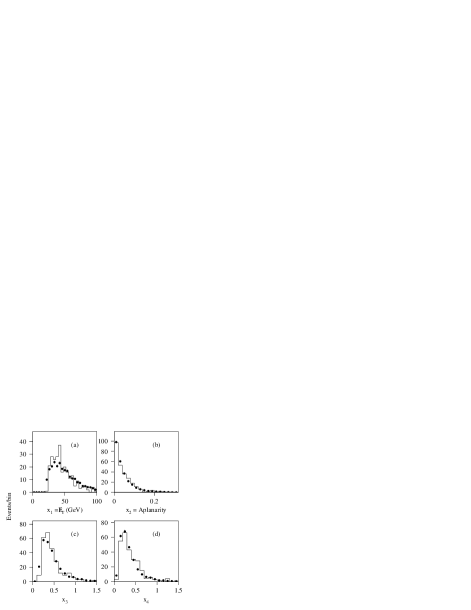
FIG. 12.: The variables $x_{1}\ldots x_{4}$ used as input to the top quark discriminants, for $W+3$ jet control samples. Histograms are data, and the circles are the expected signal + background mixture.

FIG. 13.: The variables $x_{1}\ldots x_{4}$ used as input to the top quark discriminants, for the 77-event candidate sample (histogram), $t\overline{t}$ signal plus background for $m_{t}=175\ \text{GeV}/c^{2}$ (filled circles), signal alone (open squares), and background alone (open triangles). (The normalizations are as in Fig. 2.)

B Likelihood discriminant

The correlations among the variables $x_{1}$–$x_{4}$ are small. Although we may not conclude that the variables are, as a consequence, independent, experience shows that it is frequently true that weakly correlated variables are also nearly independent. We assume this to be true for $x_{1}$–$x_{4}$ and write the functions $f_{s}$ and $f_{b}$ as

$$f_{s}({\bf x}) \equiv \prod_{i=1}^{4}s^{w_{i}}_{i}(x_{i}),$$ (12)

$$f_{b}({\bf x}) \equiv \prod_{i=1}^{4}b^{w_{i}}_{i}(x_{i}),$$ (13)

where $s_{i}(x_{i})$ and $b_{i}(x_{i})$ are the normalized distributions of variable $x_{i}$ for signal and background, respectively. These forms reduce to the usual likelihood function for strictly independent variables when the weights $w_{i}=1$. With the weights adjusted slightly away from unity, we can nullify the correlation between $m_{\text{fit}}$ and the discriminant ${\cal D}_{\text{LB}}({\bf x})$ formed from Eqs. (4) and (12), while maintaining maximal discrimination between high-mass ($>170\ \text{GeV}/c^{2}$) top events and the background. The subscript “LB” (= “low bias”) denotes the fact that cuts on ${\cal D}_{\text{LB}}$ introduce negligible bias (that is, distortion) in the $m_{\text{fit}}$ distributions.

We have found it useful to have a parameterized form for the discriminant ${\cal D}_{\text{LB}}$. Rather than directly parameterizing the functions $f_{s}$ and $f_{b}$, it is simpler to parameterize the ratio ${\cal{L}}\equiv f_{s}/f_{b}$ by using polynomial fits to the four functions ${\cal{L}}_{i}\equiv s_{i}(x_{i})/b_{i}(x_{i})$ and then computing ${\cal{L}}\equiv\exp\sum_{i}w_{i}\ln{\cal{L}}_{i}$ [24]. We then find ${\cal D}_{\text{LB}}={\cal{L}}/(1+{\cal{L}})$.

We also make use of cuts based on ${\cal D}_{\text{LB}}$ and $H_{T2}$. All tagged events pass this “LB selection”; for untagged events, we require:

• ${\cal D}_{\text{LB}}>0.43$ and

• $H_{T2}>90\ \text{GeV}$.

This selection is used in several places to separate the sample into signal-rich and background-rich portions. The cut ${\cal D}_{\text{LB}}>0.43$ was chosen to minimize the error on the top quark mass when analyzing Monte Carlo samples. The $H_{T2}$ cut removes very little signal for the top quark masses of interest (see Fig. 11), but provides an easy way of further reducing the background.

C Neural network discriminant

The variables $x_{1}$–$x_{4}$ were chosen to have minimal correlations with the fitted mass. We therefore consider a second, complementary, discriminant in which no attempt is made to nullify the correlation between the discriminant and the fitted mass. We do attempt, however, to account for the small correlations that exist among the variables $x_{1}$–$x_{4}$. This discriminant, denoted by ${\cal D}_{\text{NN}}$, is calculated with a neural network (NN) having four input nodes, three hidden nodes, and a single output node, whose value is ${\cal D}_{\text{NN}}$. The network is trained using the back-propagation algorithm provided in the program jetnet V3.0 [25] using the default training parameters. We use herwig $t\overline{t}$ Monte Carlo with $m_{t}=170\ \text{GeV}/c^{2}$ as the signal, and vecbos $W+\text{jets}$ events as the background (equal numbers of each). During training, the target outputs are set to unity for the signal and zero for the background. Under these conditions, the network output approximates the ratio $s({\bf x})/[s({\bf x})+b({\bf x})]$ [26], where $s({\bf x})$ is the normalized density for the signal and $b({\bf x})$ is the normalized density for the background. Since the correlations among $x_{1}\ldots x_{4}$ are small, as are the correlations with the fitted mass, we should anticipate that the discriminants ${\cal D}_{\text{LB}}$ and ${\cal D}_{\text{NN}}$ will provide comparable levels of signal to background discrimination. That this is true is evident, qualitatively, from Fig. 14 which compares the distributions of ${\cal D}_{\text{LB}}$ and ${\cal D}_{\text{NN}}$ for top quark events and for the mixture of $W$+jets and QCD multijet events appropriate for the precuts discussed earlier. The dependence of the discriminants on the top quark mass is indeed small, as shown in Fig. 15. In Fig. 16, we compare the distributions of the two discriminants obtained from the candidate sample to those predicted from Monte Carlo; the agreement is quite good.

FIG. 14.: The discriminant variables (a) ${\cal D}_{\text{LB}}$ and (b) ${\cal D}_{\text{NN}}$ plotted for the $m_{t}=175\ \text{GeV}/c^{2}$ $t\overline{t}$ (hatched) sample and the simulated background (unhatched). All histograms are normalized to unity.

FIG. 15.: The discriminant variables (a) ${\cal D}_{\text{LB}}$ and (b) ${\cal D}_{\text{NN}}$ for $t\overline{t}$ Monte Carlo with $m_{t}=150\ \text{GeV}/c^{2}$ (dashed lines), $m_{t}=175\ \text{GeV}/c^{2}$ (solid lines), and $m_{t}=200\ \text{GeV}/c^{2}$ (dotted lines). All histograms are normalized to unity.

FIG. 16.: The discriminant variables (a) ${\cal D}_{\text{LB}}$ and (b) ${\cal D}_{\text{NN}}$ for the 77-event candidate sample (histogram), $t\overline{t}$ signal plus background (filled circles), and background alone (open triangles). The binnings were chosen such that the predicted signal plus background distribution would be approximately flat.

Analogous to the LB selection, we will also make use of a cut on ${\cal D}_{\text{NN}}$. This “NN selection” is defined by ${\cal D}_{\text{NN}}>0.6$. This cut value yields roughly the same discrimination as the LB selection.

VII Variable-Mass Fit

A Introduction

The method used can be summarized as follows. For each event in the precut sample, we perform a constrained kinematic fit to the hypothesis $t\overline{t}\rightarrow l+\text{jets}$ to arrive at a “fitted mass” $m_{\text{fit}}$. Events which fit poorly are discarded. For each event, we also compute a top quark discriminant ${\cal D}$ (either ${\cal D}_{\text{LB}}$ or ${\cal D}_{\text{NN}}$). The events are then entered into a two-dimensional histogram in the $({\cal D},m_{\text{fit}})$ plane. Similar histograms are also constructed for a sample of background events and for signal Monte Carlo at various top quark masses. For each of these MC masses, we fit a sum of the signal and background histograms to the data histogram. This fit yields a background fraction and a corresponding likelihood value. These likelihood values are then plotted as a function of the top quark mass, and the final result extracted by fitting a quadratic function to their logarithms.

B Kinematic fit

The goal of the kinematic fit is to constrain a measured event to the hypothesis

$$p\overline{p}\rightarrow t\overline{t}+X\rightarrow(W^{+}b)(W^{-}\overline{b})+X\rightarrow(l\nu b)(q\overline{q}\overline{b})+X$$ (14)

(or the charge conjugate) and thus arrive at an estimate $m_{\text{fit}}$ of the top quark mass. There is a complication, however, in that when reconstructing the event, we do not know a priori which observed jet corresponds to which parton. In fact, due to QCD radiative effects, jet merging and splitting during reconstruction, and jet reconstruction inefficiencies, the observed jets may have no one-to-one correspondence with the unfragmented partons from the $t\overline{t}$ decay. Nevertheless, the fitted mass $m_{\text{fit}}$ constructed from the observed jets is correlated with the true top quark mass and can thus be used for a measurement; however, $m_{\text{fit}}$ should not be thought of as “the top quark mass” for a particular event.

The inputs to the fit are the kinematic parameters of the lepton, the jets, and the missing transverse energy vector $\vec{\mbox{${\hbox{$E$\kern-6.00006pt\lower-0.43057pt\hbox{/}}}_{T}$}}$. Only the four jets with the largest $E_{T}$ within $|\eta|<2.5$ are used in the fit (any additional jets are assumed to be due to initial state radiation). We parameterize electrons and jets in terms of energy $E$, azimuthal angle $\phi$, and pseudorapidity $\eta$. For muons, we parameterize the momentum in terms of $k=1/p$, since the resolution is more nearly Gaussian in that variable. The muon direction is also represented as $(\phi,\,\eta)$. Leptons and light quarks are fixed to zero mass; $b$ quarks are fixed to a mass of $5\ \text{GeV}/c^{2}$. The transverse momentum of the neutrino is taken to be $\vec{\mbox{${\hbox{$E$\kern-6.00006pt\lower-0.43057pt\hbox{/}}}_{T}$}}$. However, we do not use $\vec{\mbox{${\hbox{$E$\kern-6.00006pt\lower-0.43057pt\hbox{/}}}_{T}$}}$ directly in the fit, as it is correlated with all the other objects in the event. Instead, we use the $x$ and $y$ components of

$$\vec{k}_{T}=\vec{\mbox{${\hbox{$E$\kern-6.00006pt\lower-0.43057pt\hbox{/}}}_{T}$}}+\vec{E}_{T}^{\text{lep}}+\sum_{4\ \text{jets}}\vec{E}_{T}^{\text{jet}}.$$ (15)

This can be thought of as the transverse momentum of the $t\overline{t}$ pair. Note that this is not necessarily a small quantity if the event has more than four jets. One additional variable is needed to uniquely define the event kinematics: we take that to be the $z$-component of the neutrino momentum $p_{z}^{\nu}$. This variable is not measured, but is determined by the fit. This gives a total of 18 variables.

With this parameterization, there are three kinematic constraints which can be applied:

$$m(t\rightarrow l\nu b) = m(\overline{t}\rightarrow q\overline{q}\overline{b})$$ (16)

$$m(l\nu) = M_{W}$$ (17)

$$m(q\overline{q}) = M_{W}.$$ (18)

Three constraints and one unmeasured variable allow for a 2C fit.

Since we do not know the correspondence between jets and partons, we try all twelve distinct assignments of the four jets to the partons $(b\overline{b}qq)$. (But if the event has a $b$-tag, only the six permutations in which the tagged jet is used as a $b$ quark are considered.) Once a permutation is chosen, we apply the parton-level and $\eta$-dependent jet corrections described in Sec. IV. We apply a loose cut on the hadronic $W$ boson mass before the fit: $40<m(q\overline{q})<140\ \text{GeV}/c^{2}$. Permutations failing this cut are rejected without being fit in order to speed up the computation. We arrange the measured variables into a vector ${\bf x}^{m}$ and form the $\chi^{2}$

$$\chi^{2}=({\bf x}-{\bf x}^{m})^{T}{\bf G}({\bf x}-{\bf x}^{m}),$$ (19)

where ${\bf G}$ is the inverse error matrix. This $\chi^{2}$ is then minimized subject to the kinematic constraints of Eq. (16). The minimization algorithm uses the method of Lagrange multipliers; the nonlinear constraint equations are solved using an iterative technique. (The algorithm used is very similar to that of the squaw kinematic fitting program [27]; a detailed description may be found in Ref. [28].) If this minimization does not converge, the permutation is rejected. A permutation is also rejected if $\chi^{2}>10$. For each surviving permutation, this method gives a fitted mass $m_{\text{fit}}$ and a $\chi^{2}$. We pick the $m_{\text{fit}}$ value corresponding to the smallest $\chi^{2}$ as $m_{\text{fit}}$ for the event.

There is one additional wrinkle to the above procedure. In order to start each fit, we must specify an initial value for the unmeasured variable $p_{z}^{\nu}$. We choose it so that the two top quarks are assigned equal mass. This yields a quadratic equation for $p_{z}^{\nu}$. If the solutions are complex, the real part is used. Otherwise, there are two real solutions. Both are tried, and the fit which gives the smaller $\chi^{2}$ is retained. Note, however, that since $p_{z}^{\nu}$ does not enter into the $\chi^{2}$ (its measurement error is effectively infinite), the only effect its initial value can have on the final result is to influence which local minimum the fit will find, should there happen to be more than one. In the majority of cases, two distinct neutrino solutions yield nearly the same fit result.

The error matrix ${\bf G}^{-1}$ is taken to be diagonal. The resolutions used are given in Table VI. (The lepton angular resolutions are much smaller than the other resolutions, and can be taken to be effectively zero.) In most cases, these resolutions were derived from $t\overline{t}$ Monte Carlo events by comparing reconstructed objects to generator-level objects.

TABLE VI.: Object resolutions. The operator $\oplus$ denotes a sum in quadrature.

	Energy resolution	$\sigma(\phi)$	$\sigma(\eta)$
Electrons	${\sigma(E_{T})/E_{T}}=0.0157\oplus{0.072\ \text{GeV}^{1/2}/\sqrt{E_{T}}}\oplus{0.66\ \text{GeV}/E_{T}}$
Muons	$\sigma(1/p)=C\leavevmode\leavevmode\hbox{${}^{\rm a}$}{}\oplus{0.2/p}$
Jets
$0<|\eta_{\text{det}}|<0.8$	${\sigma(E)/E}=0.036\oplus{1.145\ \text{GeV}^{1/2}/\sqrt{E}}$	$0.04\>\text{rad}$	$0.04$
$0.8<|\eta_{\text{det}}|<1.4$	${\sigma(E)/E}=0.082\oplus{1.264\ \text{GeV}^{1/2}/\sqrt{E}}$	$0.05\>\text{rad}$	$0.05$
$1.4<|\eta_{\text{det}}|<2.0$	${\sigma(E)/E}=0.046\oplus{1.305\ \text{GeV}^{1/2}/\sqrt{E}}$	$0.05\>\text{rad}$	$0.05$
$k_{T}$	$\sigma({k_{T}}_{x})=\sigma({k_{T}}_{y})=12\ \text{GeV}$

Results of this procedure on Monte Carlo $t\overline{t}$ samples are shown in Fig. 17. Figure 17(a) shows results using the herwig partons directly, before any QCD evolution has taken place. A rather sharp peak is seen; further, about $80\%$ of the time, the permutation with the lowest $\chi^{2}$ is the one which is actually correct. The residual width seen in the plot is due mainly to the non-zero widths of the $W$ bosons. Figure 17(b) shows results from the same sample, but after QCD evolution and jet fragmentation. The final state particles are clustered together in cones of width $\Delta R=0.5$ in order to simulate the action of the jet reconstruction algorithm. This distribution is considerably broader. There are fewer events in the hatched plot because it is not always possible to uniquely define the correct permutation. Due to splitting and merging effects, jet finding inefficiencies, and jets falling below the selection threshold, the correct permutation can be uniquely identified in only about $50\%$ of events. In that case, the correct permutation is the lowest $\chi^{2}$ permutation about $40\%$ of the time. Finally, Fig. 17(c) shows results for a sample which has been through the full detector simulation and reconstruction. The resulting distribution has essentially the same width as that of Fig. 17(b); this indicates that the dominant contribution to the width of this distribution comes from QCD radiation and jet combinatoric effects, and not from the detector resolution.

FIG. 17.: Tests of kinematic fit method on $t\overline{t}$ Monte Carlo samples ($m_{t}=170\ \text{GeV}/c^{2}$, $e+\text{jets}$ channel). (a) Using herwig partons directly. (b) Final state Monte Carlo particles, after clustering into $R=0.5$ cones. (c) After full detector simulation and reconstruction. The hatched plots show the results for the correct jet permutation (regardless of whether or not it has the lowest $\chi^{2}$). Displayed means and widths are from a Gaussian fit, shown by the dashed curve.

The (MC) fit $\chi^{2}$ distributions resulting from the fit to the correct jet permutation are shown in Fig. 18. The distributions agree reasonably well with the expectations for a two degree-of-freedom $\chi^{2}$, except for a tail at the high end due to non-Gaussian tails in the resolutions. The (MC) $m_{\text{fit}}$ distributions for the four channels are shown in Fig. 19.

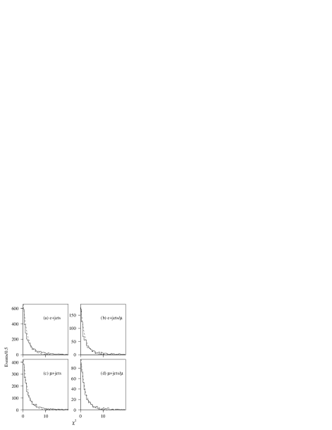
FIG. 18.: Fit $\chi^{2}$ distributions for the correct jet permutation for $t\overline{t}$ Monte Carlo samples ($m_{t}=170\ \text{GeV}/c^{2}$). The dashed curve is the $\chi^{2}$ distribution for two degrees of freedom, normalized to the area of the histogram.

FIG. 19.: Fitted mass distributions for $t\overline{t}$ Monte Carlo samples ($m_{t}=170\ \text{GeV}/c^{2}$) for the jet permutation with the lowest $\chi^{2}$. Hatched histograms show the results for the correct jet permutation (regardless of whether or not it has the lowest $\chi^{2}$). Displayed means and widths are from a Gaussian fit, shown by the dashed curve.

FIG. 20.: Fitted mass distributions for $t\overline{t}$ Monte Carlo samples ($m_{t}=170\ \text{GeV}/c^{2}$, $e+\text{jets}$ channel). With jets scaled (a) down and (b) up by $2.5\%+0.5\ \text{GeV}$. Hatched histograms show the results for the correct jet permutation (regardless of whether or not it has the lowest $\chi^{2}$). Displayed means are from a Gaussian fit, shown by the dashed curve.

Figure 20 shows the distributions which result after the jets in each Monte Carlo event are scaled up or down by the per-jet systematic error of $2.5\%+0.5\ \text{GeV}$. This shifts the fitted mass by approximately $\pm 3.7\ \text{GeV}/c^{2}$.

Figure 21 shows the fitted mass distribution for several top quark masses and for the background.

FIG. 21.: Fitted mass distributions, all channels combined. Shown is $t\overline{t}$ Monte Carlo with (a) $m_{t}=150\ \text{GeV}/c^{2}$, (b) $m_{t}=170\ \text{GeV}/c^{2}$, and (c) $m_{t}=190\ \text{GeV}/c^{2}$ and (d) background. The hatched distributions are after the LB selection is applied.

A possible objection to the fit method described here is that it does not take into account the intrinsic widths of the $W$ boson and top quark decays. To investigate this, an alternate fitting method was tried which explicitly incorporates these widths. This method is based on a standard unconstrained minimization package (minuit [29]). The quantity minimized is the $\chi^{2}$ as defined in Eq. (19) with three Breit-Wigner constraint terms added: two for the two $W$ bosons, and one for the top quark mass difference:

$${\chi^{2}}^{\prime}=\chi^{2} - 2\ln{\Gamma_{W}^{2}/4\over\Gamma_{W}^{2}/4+(m(l\nu)-M_{W})^{2}}$$ (20)

$$- 2\ln{\Gamma_{W}^{2}/4\over\Gamma_{W}^{2}/4+(m(q\overline{q})-M_{W})^{2}}$$ (21)

$$- 2\ln{\Gamma_{t}^{2}\over\Gamma_{t}^{2}+(m(l\nu b)-m(q\overline{q}\overline{b}))^{2}}.$$ (22)

(The factor of 4 difference in the last term comes from convoluting two Breit-Wigner functions centered on $m(l\nu b)$ and $m(q\overline{q}\overline{b})$.) The $W$ boson width is taken to be $2\ \text{GeV}/c^{2}$. The top quark width is taken to depend on the mass as $\Gamma_{t}=(\alpha m_{t})^{3}$; the proportionality constant $\alpha$ is set so that $\Gamma_{t}=0.6\ \text{GeV}/c^{2}$ at $m_{t}=140\ \text{GeV}/c^{2}$. (Here, $m_{t}=(m(l\nu b)+m(q\overline{q}\overline{b}))/2$.) These widths are small compared to the experimental resolutions. The results of this procedure are compared to those from the Lagrange-multiplier based fitter in Fig. 22. In most cases, the results are nearly identical, implying that neglecting the widths is not a serious problem. Since this algorithm takes several times longer to execute, it is not used further.

FIG. 22.: Differences between the results obtained from the minuit-based fitter and the Lagrange-multiplier based fitter for (a) $m_{\text{fit}}$ and (b) $\chi^{2}$. (For $t\overline{t}$ Monte Carlo with $m_{t}=170\ \text{GeV}/c^{2}$, $e+\text{jets}$ channel.)

C Likelihood fit

The next problem to be solved is the extraction of the top quark mass from the data sample, which is a mixture of signal and background. This is done using a binned Poisson-statistics maximum-likelihood fit at discrete top quark masses. (The method is described in more detail in Ref. [30].)

We bin the data according to some characteristics of the events. (For this analysis, we will be using $m_{\text{fit}}$ and either ${\cal D}_{\text{LB}}$ or ${\cal D}_{\text{NN}}$.) Call the number of bins $M$, the total number of events $N$, and the number of events in each bin $N_{j}$.

We also know the distribution expected for different values of the top quark mass, and also for the background. (This is from Monte Carlo except for the QCD multijet background.) For both the signal and background, we have a distribution of events among the $M$ bins; call the numbers of events in each bin of these distributions $A^{s}_{j}$ and $A^{b}_{j}$.

We regard these distributions as drawn from “true” distributions $a^{s}_{j}$ and $a^{b}_{j}$, and write the probability for seeing the observed data set $D$ given these parameters as a Poisson likelihood

$$L(D|A,a,p)=\prod_{j=1}^{M}q(N_{j},p_{s}a^{s}_{j}+p_{b}a^{b}_{j})\,q(A^{s}_{j},a^{s}_{j})\,q(A^{b}_{j},a^{b}_{j}),$$ (23)

where $q$ is the Poisson distribution $q(N,a)\equiv e^{-a}a^{N}/N!$ and $p_{s}$ and $p_{b}$ are the signal and background strengths. These strengths can be related to the number of expected events $n_{s}$ and $n_{b}$ by $p_{s}=n_{s}/(M+\sum_{j}A^{s}_{j})$, and similarly for $n_{b}$. (The $M$ term in the denominator ensures that the sum of the maximum likelihood estimates for $n_{s}$ and $n_{b}$ equals $N$. See Ref. [30] for further discussion. Note that usually $M\ll\sum_{j}A_{j}$.) The total number of events expected is thus $n_{j}=p_{s}a^{s}_{j}+p_{b}a^{b}_{j}$. We eliminate the $a_{j}$’s from this likelihood by integrating over them; the result is

$$L(D|A,p) = \prod_{j=1}^{M}\sum_{k=0}^{N_{j}}{p_{s}^{k}\over(1+p_{s})^{A^{s}_{j}+k+1}}{p_{b}^{N_{j}-k}\over(1+p_{b})^{A^{b}_{j}+N_{j}-k+1}}$$ (25)

$$\times{A^{s}_{j}+k\choose k}{A^{b}_{j}+N_{j}-k\choose N_{j}-k}.$$

Following Ref. [11], we then modify the likelihood by dividing by the constant factor

$$\prod_{j}q(N_{j},N_{j}).$$ (26)

This has the effect of making the quantity $-2\ln L$ behave asymptotically like a $\chi^{2}$ distribution. (Note, however, that for our experiment, the sample size is too small for this asymptotic behavior to be accurately realized.)

We now have a set of signal models, each corresponding to a different top quark mass $m_{t}$. For each signal model, we fit it plus the background to the data, yielding $n_{s}$ and $n_{b}$. A maximum likelihood fit is used, based on minuit [29]. The minimum value of $-\ln L$ is retained; call this $-\ln L_{\text{min}}$. The resulting values of $(m_{t},-\ln L_{\text{min}})$ then define a likelihood curve as a function of top quark mass.

We also define a statistical error on $-\ln L_{\text{min}}$ due to the finite Monte Carlo statistics. This is done by the simple method of taking in turn each bin $j$ in the input Monte Carlo histograms, varying the contents up or down by $\sqrt{A_{j}}$, and re-evaluating the likelihood. (To save time, the fit for $n_{s}$ and $n_{b}$ is not redone for each variation; early testing showed it to make very little difference.) The resulting variations in $-\ln L_{\text{min}}$ for each bin are then added in quadrature. This error is calculated separately for the signal and background samples; however, any effects from fluctuations in the background sample will be highly correlated from mass point to mass point. Thus, the errors shown on the plots and used in the fit below come from the signal samples only.

The final step is to extract a mass value from this set of $(m_{t},-\ln L_{\text{min}})$ points. This is done by fitting a quadratic function to the smallest $-\ln L_{\text{min}}$ and the four closest points on each side. The points are weighted by the statistical errors assigned to the $-\ln L_{\text{min}}$ values. The position of the minimum of this quadratic defines the mass estimate, and its width (where the curve has risen by $0.5$) gives an error estimate. We also want estimates for $n_{s}$ and $n_{b}$. For each mass $m_{t}$, we have a separate estimate for $n_{s}$ and $n_{b}$ returned from minuit. The final estimates of these values are determined by a linear interpolation between the two points bracketing the final $m_{t}$ estimate. The errors are found in the same manner.

For comparison, some results are also given using 11 points instead of 9 for the polynomial fit, and using a cubic function instead of a quadratic one.

D Fitting variables and binning

From each event, we derive two variables: the fitted mass $m_{\text{fit}}$ and a discriminant ${\cal D}$. We use these variables to bin the data into a two-dimensional histogram. The top quark mass is then extracted from a fit to the expectations from Monte Carlo, as described in the previous section.

Two different discriminants and histogram binnings are used. For both binnings, the fitted mass axis has twenty bins of width $10\ \text{GeV}/c^{2}$ over the range $80$ to $280\ \text{GeV}/c^{2}$. They differ in the definition of the discriminant axis. For the “LB” analysis, the discriminant axis is divided into two bins, the first bin containing events which fail the LB selection (as defined in Sec. VI B), and the second containing events which pass it. (Recall that all tagged events pass the LB selection.) For the “NN” analysis, the discriminant axis is the NN variable ${\cal D}_{\text{NN}}$. (Note that tagging information is not used in forming ${\cal D}_{\text{NN}}$.) There are ten unevenly spaced bins, as defined in Table VII. These bin boundaries were chosen so that the expected signal + background distribution populates the bins approximately uniformly. There are thus 40 bins in the LB binning, and 200 bins in the NN binning. Examples of the resulting histograms are shown in Fig. 23.

TABLE VII.: NN bin definitions.

Bin	${\cal D}_{\text{NN}}$ range
1	$0.000$ – $0.105$
2	$0.105$ – $0.166$
3	$0.166$ – $0.257$
4	$0.257$ – $0.373$
5	$0.373$ – $0.488$
6	$0.488$ – $0.595$
7	$0.595$ – $0.687$
8	$0.687$ – $0.766$
9	$0.766$ – $0.846$
10	$0.846$ – $1.000$

FIG. 23.: Monte Carlo histograms for LB and NN analyses for $t\overline{t}$ Monte Carlo with $m_{t}=175\ \text{GeV}/c^{2}$, vecbos $W+\text{jets}$ background, and QCD multijet background. More top quark-like events are towards the top of the plots.

These histograms are generated separately for each of the four channels. They are then combined using the set of fixed weights given in Table VIII. We derive these numbers by calculating the expected signal and background in each channel using the same techniques as used for the cross section measurement [8] (except that only the precuts are applied). We also combine the histograms for vecbos $W+\text{jets}$ background and the QCD multijet background using a fixed QCD fraction of $(22\pm 5)\%$, derived in the same manner.

TABLE VIII.: Fraction of events expected in each channel after the precuts.

	$e+\text{jets}$	$e+\text{jets}/\mu$	$\mu+\text{jets}$	$\mu+\text{jets}/\mu$
herwig $t\overline{t}$
$110\text{--}150\ \text{GeV}/c^{2}$	$0.376\pm 0.020$	$0.085\pm 0.013$	$0.468\pm 0.025$	$0.071\pm 0.018$
$155\text{--}170\ \text{GeV}/c^{2}$	$0.418\pm 0.018$	$0.097\pm 0.011$	$0.425\pm 0.021$	$0.059\pm 0.015$
$172\text{--}190\ \text{GeV}/c^{2}$	$0.427\pm 0.016$	$0.093\pm 0.010$	$0.409\pm 0.019$	$0.071\pm 0.013$
$195\text{--}230\ \text{GeV}/c^{2}$	$0.416\pm 0.014$	$0.097\pm 0.009$	$0.419\pm 0.018$	$0.068\pm 0.012$
vecbos	$0.531\pm 0.077$	$0.015\pm 0.017$	$0.441\pm 0.079$	$0.013\pm 0.003$
QCD	$0.443\pm 0.111$	$0.013\pm 0.030$	$0.488\pm 0.115$	$0.056\pm 0.020$

E Fits to data

The results of the kinematic fit for the candidate events are given in Tables IX through XII. (Complete details of the candidate events are available in Ref. [31].) There are $91$ events passing the precuts (PR). One of these, however, had no successful fits, and is not considered further. Thirty-six of these events then pass the LB selection. The distributions of the fitted masses of these candidates are shown in Fig. 24. When the $\chi^{2}<10$ cut is imposed, there are $77$ PR events and $31$ LB events. Distributions of their fitted masses are shown in Fig. 25. The $\chi^{2}$ distribution of the 90 events is shown in Fig. 26. It compares well to the expectation from Monte Carlo.

TABLE IX.: Kinematic fit results and top quark discriminants for events in the $e+\text{jets}$ channel for the jet permutation with the smallest $\chi^{2}$. The “Perm” column gives the assignment of the jets to partons, listed in order of decreasing jet $E_{T}$: $B_{l}$ and $B_{h}$ denote the $b$ quarks associated with the leptonically and hadronically decaying top quarks, respectively, while $W$ denotes the quarks from the hadronically decaying $W$ boson. The fitted mass $m_{\text{fit}}$ is in $\text{GeV}/c^{2}$.

Run	Event	Perm.	$m_{\text{fit}}$	$\chi^{2}$	${\cal D}_{\text{LB}}$	${\cal D}_{\text{NN}}$
c 62199	15224	$B_{l}WWB_{h}$	$265.4$	$15.9$	$0.09$	$0.21$
b c 62431	788	$WB_{h}B_{l}W$	$241.7$	$0.23$	$0.16$	$0.09$
a b c 63066	13373	$B_{l}WB_{h}W$	$206.8$	$1.35$	$0.85$	$0.95$
b c 64464	21611	$B_{h}WWB_{l}$	$115.7$	$0.64$	$0.22$	$0.31$
a b c 81949	12380	$B_{l}B_{h}WW$	$132.7$	$1.10$	$0.77$	$0.82$
b c 82024	44002	$WB_{l}B_{h}W$	$130.2$	$0.97$	$0.06$	$0.31$
b c 82220	20012	$B_{h}WB_{l}W$	$120.8$	$2.53$	$0.03$	$0.06$
82996	24461	$WB_{h}WB_{l}$	$166.8$	$31.8$	$0.73$	$0.74$
84331	13271	$B_{h}WB_{l}W$	$116.8$	$14.4$	$0.25$	$0.27$
b c 84890	28925	$B_{h}WB_{l}W$	$126.4$	$0.78$	$0.06$	$0.07$
a b c 85917	22	$B_{l}WWB_{h}$	$162.3$	$2.26$	$0.79$	$0.81$
b c 86518	11716	$B_{h}WWB_{l}$	$243.5$	$0.54$	$0.18$	$0.29$
a b c 86601	33128	$WB_{l}B_{h}W$	$179.2$	$0.39$	$0.43$	$0.29$
a b c 87063	39091	$B_{h}WB_{l}W$	$188.4$	$0.39$	$0.58$	$0.63$
b c 87104	25823	$WB_{h}B_{l}W$	$119.9$	$2.11$	$0.06$	$0.09$
b c 87329	13717	$B_{h}B_{l}WW$	$242.1$	$1.95$	$0.39$	$0.23$
b c 87446	14294	$WWB_{h}B_{l}$	$118.3$	$1.11$	$0.59$	$0.52$
88038	14829	$WWB_{h}B_{l}$	$101.0$	$12.8$	$0.37$	$0.28$
c 88044	9807	$WB_{l}WB_{h}$	$145.2$	$34.0$	$0.09$	$0.11$
a b c 88045	35311	$WB_{h}WB_{l}$	$178.2$	$2.71$	$0.83$	$0.81$
b c 88125	15437	$WB_{h}WB_{l}$	$115.9$	$0.16$	$0.78$	$0.74$
b c 88463	3627	$WB_{h}WB_{l}$	$111.7$	$9.93$	$0.16$	$0.46$
b 88588	15993	$WWB_{h}B_{l}$	$103.4$	$7.44$	$0.29$	$0.30$
a b c 89484	11741	$B_{h}B_{l}WW$	$135.0$	$0.76$	$0.53$	$0.58$
b c 89550	18042	$WWB_{h}B_{l}$	$103.5$	$0.07$	$0.30$	$0.27$
a 89708	24871	$WB_{h}B_{l}W$	$144.6$	$20.1$	$0.62$	$0.74$
a b c 89936	6306	$WB_{h}B_{l}W$	$220.4$	$1.29$	$0.50$	$0.68$
a b c 89972	13657	$WB_{h}B_{l}W$	$176.7$	$9.08$	$0.65$	$0.77$
b c 90108	31611	$WB_{h}WB_{l}$	$137.4$	$0.41$	$0.21$	$0.21$
b c 90435	32258	$B_{h}B_{l}WW$	$154.1$	$1.05$	$0.27$	$0.62$
b c 90496	28296	$B_{h}WB_{l}W$	$112.9$	$0.28$	$0.23$	$0.19$
b 90693	8678	$B_{h}B_{l}WW$	$105.5$	$8.98$	$0.51$	$0.27$
c 90795	14246	$B_{h}WB_{l}W$	$193.9$	$12.8$	$0.09$	$0.07$
b c 90804	6474	$WWB_{l}B_{h}$	$114.2$	$0.64$	$0.34$	$0.59$
b c 91923	502	$WB_{h}WB_{l}$	$162.1$	$0.14$	$0.09$	$0.15$
b c 92013	11825	$WB_{h}B_{l}W$	$134.1$	$3.68$	$0.11$	$0.15$
b c 92217	109	$WWB_{h}B_{l}$	$107.8$	$0.58$	$0.77$	$0.82$
b c 92278	21744	$WB_{h}WB_{l}$	$125.9$	$7.26$	$0.17$	$0.31$
a b c 92673	4679	$B_{l}B_{h}WW$	$267.7$	$1.85$	$0.92$	$0.97$
b c 94750	4683	$B_{h}WWB_{l}$	$201.5$	$3.63$	$0.32$	$0.49$
a 96329	13811		$---$		$0.54$	$0.79$
b c 96676	79957	$WB_{l}B_{h}W$	$224.1$	$0.47$	$0.36$	$0.46$
a b c 96738	27592	$B_{l}WWB_{h}$	$236.6$	$5.68$	$0.60$	$0.83$

TABLE X.: Same as Table IX for the $\mu+\text{jets}$ channel.

Run	Event	Perm.	$m_{\text{fit}}$	$\chi^{2}$	${\cal D}_{\text{LB}}$	${\cal D}_{\text{NN}}$
b c 61514	4537	$B_{h}WB_{l}W$	$120.8$	$3.40$	$0.26$	$0.59$
a b c 63183	13926	$WWB_{h}B_{l}$	$133.7$	$1.26$	$0.84$	$0.83$
a b c 63740	14197	$B_{l}WB_{h}W$	$185.3$	$2.56$	$0.94$	$0.96$
b c 80703	31477	$WB_{h}B_{l}W$	$167.2$	$0.54$	$0.24$	$0.40$
a b c 81909	11966	$B_{h}WB_{l}W$	$162.9$	$1.11$	$0.67$	$0.66$
b 81949	13778	$WB_{h}WB_{l}$	$109.2$	$8.25$	$0.27$	$0.25$
b c 82639	11573	$WB_{l}WB_{h}$	$117.3$	$2.24$	$0.35$	$0.47$
a b c 82694	25595	$WB_{l}WB_{h}$	$114.0$	$2.03$	$0.56$	$0.53$
a b c 84696	29253	$WB_{h}B_{l}W$	$221.0$	$1.05$	$0.74$	$0.89$
b c 84728	18171	$B_{h}B_{l}WW$	$136.0$	$3.65$	$0.40$	$0.38$
b c 85888	28599	$B_{h}WWB_{l}$	$189.6$	$5.78$	$0.18$	$0.09$
a b c 87063	14368	$WWB_{h}B_{l}$	$182.1$	$0.02$	$0.50$	$0.72$
87604	14282	$B_{l}WWB_{h}$	$90.6$	$40.6$	$0.14$	$0.38$
a c 87820	6196	$B_{h}B_{l}WW$	$178.0$	$17.8$	$0.87$	$0.97$
a b c 88464	2832	$B_{h}WB_{l}W$	$154.1$	$0.14$	$0.87$	$0.93$
a b c 88530	7800	$WB_{l}B_{h}W$	$151.2$	$0.08$	$0.62$	$0.60$
88597	1145	$WWB_{h}B_{l}$	$124.6$	$10.2$	$0.20$	$0.42$
b c 88603	2131	$WB_{l}WB_{h}$	$123.7$	$0.66$	$0.13$	$0.17$
b c 89751	27345	$B_{h}WWB_{l}$	$132.4$	$1.14$	$0.15$	$0.14$
a b c 89943	19016	$WB_{h}B_{l}W$	$163.7$	$0.03$	$0.65$	$0.74$
b c 90133	14110	$WB_{h}WB_{l}$	$169.4$	$4.88$	$0.26$	$0.28$
a b c 90660	20166	$WB_{l}B_{h}W$	$222.6$	$1.28$	$0.70$	$0.90$
a b c 90690	12392	$B_{h}WB_{l}W$	$153.3$	$0.58$	$0.70$	$0.78$
b c 90836	14924	$WB_{l}WB_{h}$	$147.4$	$3.13$	$0.07$	$0.08$
b c 90864	17697	$WB_{h}WB_{l}$	$96.6$	$0.81$	$0.44$	$0.62$
b c 91359	15030	$WB_{h}WB_{l}$	$118.9$	$1.81$	$0.54$	$0.60$
b c 92081	3825	$WB_{h}B_{l}W$	$117.7$	$3.72$	$0.07$	$0.40$
b c 92082	34466	$WB_{h}B_{l}W$	$176.2$	$0.30$	$0.31$	$0.49$
a 92114	1243	$WB_{l}B_{h}W$	$187.0$	$11.7$	$0.96$	$0.96$
a b c 92126	21544	$B_{l}WWB_{h}$	$157.2$	$0.02$	$0.82$	$0.91$
b c 92142	27042	$WB_{l}B_{h}W$	$148.7$	$4.71$	$0.24$	$0.21$
b c 92226	34133	$WB_{h}B_{l}W$	$140.3$	$0.49$	$0.41$	$0.66$
b c 92714	4141	$WWB_{h}B_{l}$	$106.4$	$6.28$	$0.43$	$0.59$
a b c 92714	12581	$B_{l}B_{h}WW$	$166.3$	$1.66$	$0.57$	$0.66$
b c 94750	1147	$WWB_{l}B_{h}$	$126.9$	$0.82$	$0.32$	$0.23$
b c 96258	2707	$B_{l}WB_{h}W$	$171.2$	$1.02$	$0.49$	$0.28$
b c 96264	93611	$B_{h}WWB_{l}$	$111.7$	$0.41$	$0.06$	$0.14$
b c 96280	14555	$WB_{h}B_{l}W$	$133.8$	$0.07$	$0.69$	$0.68$
b c 96287	20104	$WB_{h}B_{l}W$	$182.5$	$5.64$	$0.16$	$0.14$
a b c 96399	32921	$B_{l}B_{h}WW$	$172.8$	$0.28$	$0.68$	$0.83$
a b c 96591	39318	$B_{h}B_{l}WW$	$174.3$	$0.94$	$0.55$	$0.75$

TABLE XI.: Same as Table IX for the $e+\text{jets}/\mu$ channel.

Run	Event	Perm.	$m_{\text{fit}}$	$\chi^{2}$	${\cal D}_{\text{LB}}$	${\cal D}_{\text{NN}}$
a 62199	13305	$B_{l}B_{h}WW$	$173.2$	$40.0$	$0.55$	$0.61$
a b c 85129	19079	$WB_{l}B_{h}W$	$137.0$	$0.93$	$0.81$	$0.85$
a b c 86570	8642	$B_{h}WWB_{l}$	$144.5$	$0.66$	$0.74$	$0.29$
a 89372	12467	$B_{h}WWB_{l}$	$186.6$	$22.1$	$0.23$	$0.25$

TABLE XII.: Same as Table IX for the $\mu+\text{jets}/\mu$ channel.

Run	Event	Perm.	$m_{\text{fit}}$	$\chi^{2}$	${\cal D}_{\text{LB}}$	${\cal D}_{\text{NN}}$
a b c 58203	4980	$WB_{h}B_{l}W$	$138.3$	$0.25$	$0.56$	$0.62$
a b c 91712	22	$B_{h}WB_{l}W$	$203.3$	$0.44$	$0.51$	$0.44$
a b c 92704	14022	$WB_{h}B_{l}W$	$175.8$	$0.11$	$0.79$	$0.88$

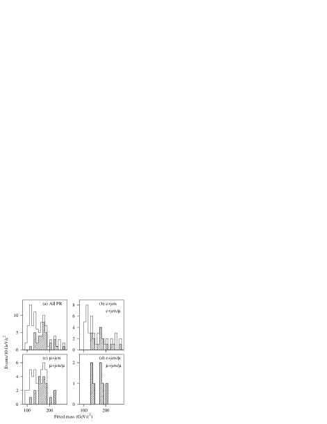
FIG. 24.: Fitted mass distributions for candidate events. The hatched histograms show the LB subsample.

FIG. 25.: Fitted mass distributions for candidate events with $\chi^{2}<10$. The hatched histograms show the LB subsample.

FIG. 26.: Fit $\chi^{2}$ distribution from data (histogram), the expected $t\overline{t}$ signal + background (filled circles), and background alone (open triangles).

Results of likelihood fits to the data sample are shown in Table XIII. Several methods of extracting the final top quark mass are tabulated. The labels “quad$N$” and “cub$N$” denote, respectively, $N$-point quadratic and cubic fits to the negative log likelihood values. The reported central value is the minimum of the fit curve, and the error indicated is the width of the curve where it has risen by $0.5$ from the minimum. For the “avg” fits, the central value is the mean of the likelihood curve (calculated using trapezoidal-rule integration), and the reported error on the mass is the symmetric interval around the mean containing $68\%$ of the likelihood. Table XIII also shows the result for the “NN2” binning. This is a variant of the NN binning which uses only two bins in ${\cal D}_{\text{NN}}$: both the first six bins and the last four bins are coalesced. The result is seen to be consistent with the 10-bin NN analysis.

For our final result, we use the nine-point quadratic fit. This choice is motivated by a desire to use a simple functional form; furthermore, it will be seen in the next section that among the polynomial fits considered, it gives the slope closest to unity when one plots extracted mass versus Monte Carlo input mass. The resulting mass is then $174.0\pm 5.6\ \text{GeV}/c^{2}$ for the LB binning, and $171.3\pm 6.0\ \text{GeV}/c^{2}$ for NN. These fit results are exhibited in Figs. 27–30.

Note in Fig. 28 that $-\ln L$ tends to flatten out away from the minimum. Due to this, we limit the polynomial fit to the central region, where $-\ln L$ is most nearly quadratic. This flattening is related to the fact that we do not impose an external constraint on the number of signal or background events in the likelihood fit. If such a constraint is imposed, as was done in Ref. [4], the $-\ln L$ curve shows less tendency to flatten.

To use more likelihood points in the fit, a functional form which can model this flattening is needed. One such function which we investigated is

$$F(x)=-\ln(P_{1} + P_{2}g(x-P_{5},P_{8})$$ (27)

$$+ P_{3}g(x-P_{6},2P_{8})$$ (28)

$$+ P_{4}g(x-P_{7},4P_{8})),$$ (29)

where $g$ is the Gaussian form $g(x,\sigma)=\exp(-(x/\sigma)^{2}/2)$. We determine the parameters $P_{1}$–$P_{8}$ by fitting this function (using minuit) to the likelihood points over the entire range of 110–$230\ \text{GeV}/c^{2}$; the results are plotted in Fig. 28. If we extract from these curves the positions of the minima, the results are $173.6^{+5.6}_{-5.5}\ \text{GeV}/c^{2}$ for LB and $172.4^{+4.1}_{-4.2}\ \text{GeV}/c^{2}$ for NN (taking the error from where the curve rises by 0.5). From this, we conclude that the procedure of fitting a quadratic in the central region does not seriously underestimate the width. In addition, in Monte Carlo studies, $F(x)$ did not perform better on average than the simple quadratic fit; thus, we do not use $F(x)$ for the final mass extraction.

TABLE XIII.: Results of fits to the candidate sample, showing the top quark mass $m_{t}$ and the number of signal and background events $n_{s}$ and $n_{b}$. The labels “quad$N$” and “cub$N$” denote $N$-point quadratic and cubic fits, while “avg” denotes the mean value of the posterior mass probability distribution. “$-\ln L_{\text{min}}$” is the minimum $-\ln L$ point; $\chi^{2}_{\text{poly}}$ is for the polynomial fit to the likelihood points.

Binning	$-\ln L_{\text{min}}$	Method	$m_{t}$	$n_{s}$	$n_{b}$	$\chi^{2}_{\text{poly}}$
			($\text{GeV}/c^{2}$)
LB	$23.1$	quad9	$174.0^{+5.6}_{-5.6}$	$23.8^{+8.3}_{-7.8}$	$53.2^{+10.7}_{-9.3}$	$4.7$
		quad11	$174.3^{+7.5}_{-7.5}$	$23.8^{+8.5}_{-9.1}$	$53.2^{+12.2}_{-9.4}$	$29.7$
		cub9	$173.7^{+5.7}_{-5.4}$	$23.8^{+8.3}_{-7.8}$	$53.2^{+10.7}_{-9.3}$	$4.5$
		cub11	$172.4^{+6.4}_{-5.4}$	$23.8^{+8.5}_{-7.8}$	$53.2^{+10.7}_{-9.4}$	$14.7$
		avg	$175.4^{+7.7}_{-7.7}$	$23.7^{+8.5}_{-9.2}$	$53.3^{+12.4}_{-9.5}$
NN	$74.5$	quad9	$171.3^{+6.0}_{-6.0}$	$28.8^{+8.4}_{-9.1}$	$48.2^{+11.4}_{-8.7}$	$8.4$
		quad11	$170.8^{+6.1}_{-6.1}$	$29.1^{+8.2}_{-9.3}$	$47.9^{+11.6}_{-8.5}$	$9.9$
		cub9	$173.7^{+3.7}_{-4.7}$	$28.0^{+9.7}_{-8.4}$	$49.0^{+10.7}_{-10.0}$	$3.9$
		cub11	$172.5^{+4.8}_{-5.5}$	$28.3^{+9.0}_{-8.6}$	$48.7^{+10.9}_{-9.4}$	$6.3$
		avg	$170.7^{+6.7}_{-6.7}$	$29.2^{+8.4}_{-9.5}$	$47.8^{+11.8}_{-8.7}$
NN2	$29.8$	quad9	$172.0^{+5.5}_{-5.5}$	$28.4^{+9.6}_{-9.0}$	$48.6^{+11.3}_{-9.9}$	$5.7$

FIG. 27.: Fitted mass for all events which pass the precuts and the $\chi^{2}$ cut. Filled circles are a mixture of $t\overline{t}$ signal and background and open triangles are the background only, both averaged between the results of the LB and NN analyses.

FIG. 28.: Negative log likelihood for (a) LB and (b) NN analyses. The solid curve is a quadratic fit to the 9 points around the minimum; the dashed curve is from fitting Eq. (27) to all points in the range 110–$230\ \text{GeV}/c^{2}$. (c) Results of the LB fit for events passing the LB selection. The histogram is data, filled circles are a mixture of $m_{t}=175\ \text{GeV}/c^{2}$ $t\overline{t}$ signal and background, normalized using the results of the LB fit, and open triangles are background only.

FIG. 29.: Results of the LB fit for events failing the LB selection. The histogram is data, filled circles are a mixture of $m_{t}=175\ \text{GeV}/c^{2}$ $t\overline{t}$ signal and background, normalized using the results of the LB fit, and open triangles are background only.

FIG. 30.: Results of NN fit: (a) Data, (b) $m_{t}=172\ \text{GeV}/c^{2}$ $t\overline{t}$ signal plus background, normalized using the results of the NN fit.

We have explored some additional variations in the definition of the likelihood function. The algorithm of hmcmll [32] starts with the same likelihood as Eq. (23), but eliminates the nuisance parameters $a_{j}^{s}$ and $a_{j}^{b}$ using a maximum likelihood estimate rather than integration. To be able to compare likelihoods from different Monte Carlo samples, though, we modify the likelihood following the prescription of Ref. [11]:

$$L_{\lambda}={L\over\prod_{j}q(N_{j},N_{j})q(A_{j}^{s},A_{j}^{s})q(A_{j}^{b},A_{j}^{b})}.$$ (30)

The results of this procedure are given in Table XIV. Alternatively, we can eliminate $n_{s}$ and $n_{b}$ by integrating over them, rather than by using a maximum likelihood estimate. The results of this are also given in Table XIV. These variations do not have a large effect on the final result.

To further test the stability of these results, we repeat the fits using samples in which one candidate event is removed, for a total of 77 distinct fits. For the LB case, the RMS of the resulting distribution of fits was $0.3\ \text{GeV}/c^{2}$; the smallest result seen was $173.0\ \text{GeV}/c^{2}$, and the largest was $174.7\ \text{GeV}/c^{2}$. For the NN case, the RMS was $0.5\ \text{GeV}/c^{2}$, the smallest result was $170.1\ \text{GeV}/c^{2}$, and the largest was $172.5\ \text{GeV}/c^{2}$.

To summarize the main results of this section, the LB analysis yields $m_{t}=174.0\pm 5.6\ \text{GeV}/c^{2}$, and the NN analysis yields $m_{t}=171.3\pm 6.0\ \text{GeV}/c^{2}$.

TABLE XIV.: Additional fit results.

Method	Binning	$-\ln L_{\text{min}}$	$m_{t}$	$n_{s}$	$n_{b}$
			($\text{GeV}/c^{2}$)
hmcmll	LB	$22.7$	$174.1^{+5.6}_{-5.6}$	$23.6^{+7.9}_{-8.2}$	$53.4^{+10.3}_{-9.7}$
	NN	$73.1$	$172.0^{+5.1}_{-5.1}$	$34.0^{+1.9}_{-14.3}$	$42.6^{+16.0}_{-2.7}$
Integration	LB	$17.2$	$174.5^{+7.6}_{-7.6}$	$24.9^{+8.1}_{-9.7}$	$54.2^{+12.0}_{-9.9}$
	NN	$68.5$	$169.8^{+7.3}_{-7.3}$	$30.6^{+8.4}_{-10.2}$	$48.5^{+11.7}_{-9.4}$

F Tests with Monte Carlo samples

We test the mass extraction procedure by performing fits to ensembles of Monte Carlo experiments of known composition. The size of the experiments is fixed; the number of background events in each is chosen from a binomial distribution with a fixed mean.

For the first set of tests, the ensembles consist of 1000 experiments with a composition of $\left\langle n_{s}\right\rangle=26$ and $\left\langle n_{b}\right\rangle=52$, for an experiment size of $N=78$ events with a 1:2 signal/background ratio. Results for the LB and NN analyses are shown in Tables XV and XVI. For these tests, the tabulated mean value is from a Gaussian fit to the extracted mass distribution, and the width is the symmetric interval around the mean which contains $68\%$ of the entries. (We estimate the statistical errors on these means and widths to be in the range $0.5$–$1.0\ \text{GeV}/c^{2}$.) Note that the 9-point quadratic fit gives the slope closest to unity. Some results for ensembles containing signal only are given in Tables XVII and XVIII.

TABLE XV.: Ensemble tests for the LB analysis with 1:2 signal/background, showing means and $68\%$ widths. “Slope” is from a linear fit to the means.

Input	quad9		quad11		cub9		cub11
Mass	$mean$	$width$	$mean$	$width$	$mean$	$width$	$mean$	$width$
($\text{GeV}/c^{2}$)	($\text{GeV}/c^{2}$)		($\text{GeV}/c^{2}$)		($\text{GeV}/c^{2}$)		($\text{GeV}/c^{2}$)
150	$150.4$	$10.7$	$150.8$	$11.1$	$151.5$	$10.3$	$151.9$	$10.9$
155	$155.2$	$9.1$	$155.3$	$9.8$	$155.3$	$9.0$	$156.5$	$8.4$
160	$160.7$	$9.2$	$160.9$	$9.1$	$160.9$	$9.3$	$161.4$	$8.3$
162	$162.6$	$8.5$	$162.8$	$8.5$	$162.8$	$9.0$	$162.9$	$8.3$
165	$165.1$	$9.0$	$165.3$	$9.0$	$165.2$	$8.7$	$165.3$	$8.7$
168	$168.2$	$9.3$	$168.3$	$9.3$	$168.1$	$9.0$	$168.1$	$9.0$
170	$168.9$	$7.6$	$169.0$	$7.7$	$169.2$	$7.2$	$169.1$	$7.4$
172	$172.2$	$7.4$	$172.2$	$7.8$	$172.0$	$7.4$	$172.1$	$7.5$
175	$174.9$	$8.4$	$174.9$	$8.5$	$174.9$	$8.4$	$174.7$	$8.3$
178	$177.6$	$8.5$	$177.5$	$8.5$	$177.4$	$8.0$	$177.2$	$8.0$
180	$179.7$	$8.7$	$179.6$	$8.6$	$179.4$	$8.2$	$179.2$	$8.1$
182	$181.8$	$8.1$	$182.1$	$8.2$	$181.3$	$7.8$	$181.1$	$7.5$
185	$183.9$	$8.9$	$183.9$	$9.1$	$183.3$	$8.2$	$183.2$	$8.1$
190	$190.5$	$9.7$	$191.1$	$10.0$	$189.0$	$9.0$	$189.0$	$8.9$
Slope	$0.98$		$0.98$		$0.94$		$0.91$

TABLE XVI.: Same as Table XV for the NN analysis.

Input	quad9		quad11		cub9		cub11
Mass	$mean$	$width$	$mean$	$width$	$mean$	$width$	$mean$	$width$
($\text{GeV}/c^{2}$)	($\text{GeV}/c^{2}$)		($\text{GeV}/c^{2}$)		($\text{GeV}/c^{2}$)		($\text{GeV}/c^{2}$)
150	$149.0$	$9.8$	$150.1$	$10.8$	$150.0$	$8.9$	$150.8$	$9.9$
155	$154.6$	$9.6$	$154.6$	$10.0$	$155.1$	$8.6$	$155.5$	$8.2$
160	$159.6$	$9.5$	$159.8$	$9.7$	$159.6$	$9.4$	$160.1$	$8.7$
162	$161.8$	$9.2$	$162.1$	$9.0$	$161.9$	$9.1$	$162.3$	$8.3$
165	$163.9$	$9.2$	$164.4$	$9.4$	$163.7$	$9.2$	$164.0$	$8.6$
168	$167.2$	$9.7$	$167.6$	$10.0$	$166.9$	$9.8$	$167.0$	$9.8$
170	$168.3$	$8.8$	$168.3$	$8.2$	$168.4$	$8.0$	$168.3$	$8.0$
172	$171.6$	$8.8$	$171.5$	$8.3$	$171.7$	$8.4$	$171.7$	$8.3$
175	$174.6$	$9.3$	$174.6$	$9.1$	$174.5$	$9.0$	$174.3$	$9.0$
178	$176.6$	$8.7$	$176.6$	$8.8$	$176.6$	$8.6$	$176.6$	$8.4$
180	$179.0$	$9.0$	$178.9$	$8.9$	$178.6$	$8.7$	$179.0$	$8.5$
182	$181.1$	$8.9$	$180.9$	$9.0$	$180.8$	$8.4$	$180.9$	$7.8$
185	$183.0$	$8.9$	$182.8$	$9.1$	$182.8$	$8.6$	$182.5$	$8.4$
190	$189.0$	$9.1$	$189.0$	$9.8$	$188.4$	$8.5$	$188.2$	$8.1$
Slope	$0.98$		$0.96$		$0.95$		$0.93$

TABLE XVII.: Ensemble tests for the LB analysis with $n_{s}=26$ events and $n_{b}=0$.

Input	quad9		quad11		cub9		cub11
Mass	$mean$	$width$	$mean$	$width$	$mean$	$width$	$mean$	$width$
($\text{GeV}/c^{2}$)	($\text{GeV}/c^{2}$)		($\text{GeV}/c^{2}$)		($\text{GeV}/c^{2}$)		($\text{GeV}/c^{2}$)
168	$168.3$	$6.7$	$168.2$	$6.7$	$168.4$	$6.3$	$168.2$	$6.5$
170	$168.9$	$5.9$	$168.9$	$6.2$	$169.1$	$5.7$	$168.9$	$5.8$
172	$172.2$	$6.2$	$172.2$	$6.0$	$172.1$	$5.9$	$172.1$	$5.9$
175	$175.6$	$6.6$	$175.7$	$6.8$	$175.5$	$6.2$	$175.5$	$6.4$

TABLE XVIII.: Same as Table XVII for the NN analysis.

Input	quad9		quad11		cub9		cub11
Mass	$mean$	$width$	$mean$	$width$	$mean$	$width$	$mean$	$width$
($\text{GeV}/c^{2}$)	($\text{GeV}/c^{2}$)		($\text{GeV}/c^{2}$)		($\text{GeV}/c^{2}$)		($\text{GeV}/c^{2}$)
168	$167.7$	$6.3$	$168.1$	$6.8$	$168.0$	$5.8$	$167.9$	$6.4$
170	$168.9$	$6.1$	$169.0$	$6.0$	$169.0$	$5.6$	$168.8$	$5.7$
172	$172.0$	$6.1$	$172.3$	$6.2$	$172.0$	$5.5$	$172.0$	$5.9$
175	$175.6$	$6.5$	$175.6$	$6.7$	$175.2$	$6.0$	$175.3$	$6.4$

There are several competing factors which contribute to the mass dependence of the width of the ensemble mass distributions $\sigma(m_{t})$ observed in Tables XV and XVI. As $m_{t}$ increases, the widths of the $m_{\text{fit}}$ distributions slowly increase. From this one would expect the $\sigma(m_{t})$ to increase with increasing top quark mass. However, we rely on the difference between the signal and background $m_{\text{fit}}$ distributions to set the background normalization. This difference is smallest for $m_{t}$ around $140$–$150\ \text{GeV}/c^{2}$; thus, one would expect $\sigma(m_{t})$ to be larger in that region. Finally, the spacing of the generated Monte Carlo points is finer in the region near $170\ \text{GeV}/c^{2}$; the available statistics are also larger there. This permits a more accurate determination of the top quark mass in that region, leading to a smaller $\sigma(m_{t})$.

Next, we try ensembles with compositions that match the results of the likelihood fit. The results are given in Table XIX. (These and all subsequent results use the “quad9” prescription.) Plots of the mass distributions from these ensembles are shown in Fig. 31. Also shown are the distributions of the pull quantity

$$\text{pull}={m_{t}(\text{measured})-m_{t}(\text{true})\over\sigma(m_{t})}.$$ (31)

If the errors produced by the mass extraction procedure are correct, these distributions should have unit width, as is indeed observed. In addition, $70\%$ of the $1\sigma$ error intervals from the LB ensemble include $175\ \text{GeV}/c^{2}$, and $69\%$ of those from the NN ensemble include $172\ \text{GeV}/c^{2}$, as expected.

TABLE XIX.: Results of mass fits to ensembles of Monte Carlo events. The ensembles consisted of 10,000 experiments of 77 events each, with the compositions indicated below.

	Input
	Mass	$\left\langle n_{s}\right\rangle$	$\left\langle n_{b}\right\rangle$	Mean	Width
	($\text{GeV}/c^{2}$)			($\text{GeV}/c^{2}$)	($\text{GeV}/c^{2}$)
LB	$175$	$23.8$	$53.2$	$175.0$	$8.7$
NN	$172$	$28.8$	$48.2$	$171.6$	$8.0$

FIG. 31.: Mass and pull distributions for 10,000 MC experiment ensembles with compositions matching the fit results. The dashed curves are Gaussian fits. For the mass distributions, the width is the symmetric interval containing $68\%$ of the entries; for the pull distributions, it is from the Gaussian fit.

FIG. 32.: Minimum $-\ln L$ distributions from the LB and NN ensembles. The arrows show the values corresponding to the data fits.

The minimum $-\ln L$ value for the LB fit was $23.1$; for the NN fit, it was $74.5$. (A smaller value of $-\ln L$ corresponds to a better fit to the expected distributions.) This quantity is plotted for the LB and NN ensembles in Fig. 32. A $-\ln L$ value larger than that of the data is seen in about $7\%$ of LB experiments and in about $28\%$ of NN experiments.

FIG. 33.: Statistical error distributions from the LB and NN ensembles. The arrows show the values corresponding to the data fits.

One can also look at the distribution of statistical errors from ensemble tests. For the data, the statistical error is $5.6\ \text{GeV}/c^{2}$ for the LB analysis, and $6.0\ \text{GeV}/c^{2}$ for the NN analysis. Plots of the statistical error for the ensemble fits are shown in Fig. 33. An error smaller than that for the data is seen in about $6\%$ of LB experiments and in about $25\%$ of NN experiments. The correlation between the mass and the error for the LB ensemble is exhibited in Fig. 34. This shows that experiments with a small error typically yield masses closer to the true value.

FIG. 34.: Scatter plot of masses and statistical errors from the LB ensemble. The dashed lines of constant relative error delimit the “accurate subset” (see text).

It is interesting to examine the ensemble results for that subset of experiments where the extracted statistical error is similar to that actually obtained. We define this “accurate subset” as follows. First, find the relative error ($\sigma(m_{t})/m_{t}$) for the result. For LB, this is $0.0322$; for NN, it is $0.0350$. Then convert these numbers to a percentile in the relative error distribution. These are $6.0\%$ and $24.9\%$ for LB and NN, respectively. For any ensemble, we then define the accurate subset by looking at its relative error distribution and selecting those experiments which lie within a range of $\pm 5\%$ around the above percentiles. This is illustrated in Figs. 34–35. This procedure thus selects $10\%$ of the total sample. (The relative error is used because the statistical error tends to increase slightly with increasing mass; therefore, cutting on relative rather than absolute error results in a less biased subsample.)

FIG. 35.: Relative error ($\sigma(m_{t})/m_{t}$) distributions from the LB and NN ensembles. The arrows show the value corresponding to the data fits, and the hatched regions show the definitions of the accurate subsets.

There is an additional complication which arises when a cut is made on the statistical error. The spacing of the generated mass points is finer around $m_{t}=175\ \text{GeV}/c^{2}$. This permits a more accurate determination of the top quark mass in that range. However, this implies that if a small error is required, the masses of the selected events will be biased towards the region with finer spacing. (Note, however, that as long as a cut on the error is not made, the uneven MC spacing does not bias the mass. Studies of an even but coarser MC spacing show that adding extra points reduces the statistical error in the region where the extra points are added, but does not, on average, shift the extracted mass distribution.) Thus, for the accurate subset fits we changed the procedure slightly, adding Monte Carlo points at intervals of $2.5\ \text{GeV}/c^{2}$ between 130 and $160\ \text{GeV}/c^{2}$ and also between 185 and $210\ \text{GeV}/c^{2}$. These additional mass points were constructed by interpolating between the existing MC histograms on either side. The results of these fits with the accurate subset cuts are shown in Fig. 36. The widths are $4.6\ \text{GeV}/c^{2}$ and $6.0\ \text{GeV}/c^{2}$ for LB and NN, respectively. This is a further indication that the error estimates from the likelihood fit are reliable.

FIG. 36.: Mass distributions for accurate subsets of ensembles. The dashed curves are Gaussian fits.

The results of the LB and NN analyses can be compared experiment-by-experiment, provided that the ensemble definitions are the same. We use the same ensemble definition as for the first set of tests ($N=78$ events and a 1:2 signal/background ratio) with $m_{t}=175\ \text{GeV}/c^{2}$. The results for 10,000 experiments are given in Table XX. It is seen that given the observed statistical errors, a difference between the two analyses of the magnitude seen is expected $\sim 20\%$ of the time.

TABLE XX.: Comparisons of LB and NN ensembles for $m_{t}=175\ \text{GeV}/c^{2}$ and a 1:2 signal/background ratio. The first line is the mean difference between the results; the second and third lines give the fraction of experiments for which the difference exceeds the observed difference of $2.7\ \text{GeV}/c^{2}$. (Numbers are in $\text{GeV}/c^{2}$.)

	Full	LB	NN
	ensemble	acc. subset	acc. subset
$\left\langle\hbox{LB}-\hbox{NN}\right\rangle$	$0.78\pm 0.05$	$0.34\pm 0.06$	$0.51\pm 0.09$
$(\hbox{LB}-\hbox{NN})>2.7$	$29\%$	$11\%$	$18\%$
$|\hbox{LB}-\hbox{NN}|>2.7$	$45\%$	$16\%$	$28\%$

It is also interesting to look at the correlation between the LB and NN measurements. This can be defined using the ensemble mass distributions of $m_{\text{LB}}$ and $m_{\text{NN}}$ as

$$\rho={\left\langle\left(m_{\text{LB}}-\left\langle m_{\text{LB}}\right\rangle\right)\left(m_{\text{NN}}-\left\langle m_{\text{NN}}\right\rangle\right)\right\rangle\over\sigma_{\text{LB}}\sigma_{\text{NN}}}.$$ (32)

This is appropriate for Gaussian distributions; however, our distributions typically have a small number of non-Gaussian outliers. To explore the sensitivity of this quantity to these outliers, the following procedure is used.

• For the cuts of interest, plot $m_{\text{LB}}$ and $m_{\text{NN}}$. Record the means and RMS widths of these distributions ($\left\langle m_{\text{LB}}\right\rangle$, $\sigma_{\text{LB}}$, $\left\langle m_{\text{NN}}\right\rangle$, $\sigma_{\text{NN}}$).

• Reject experiments which are more than $K\sigma$ from the mean. Specifically, make the additional cut that

  $$|m_{\text{LB}}-\left\langle m_{\text{LB}}\right\rangle| < K\sigma_{\text{LB}}\quad\text{and}$$ (33)

  $$|m_{\text{NN}}-\left\langle m_{\text{NN}}\right\rangle| < K\sigma_{\text{NN}}.$$ (34)

• Replot $m_{\text{LB}}$ and $m_{\text{NN}}$ with this additional cut, and record the new means and RMS widths ($\left\langle m_{\text{LB}}\right\rangle^{\prime}$, $\sigma_{\text{LB}}^{\prime}$, $\left\langle m_{\text{NN}}\right\rangle^{\prime}$, $\sigma_{\text{NN}}^{\prime}$).

• Plot (with all cuts) the distribution of

  $$\left(m_{\text{LB}}-\left\langle m_{\text{LB}}\right\rangle^{\prime}\right)\cdot\left(m_{\text{NN}}-\left\langle m_{\text{NN}}\right\rangle^{\prime}\right).$$ (35)

• Find the mean of this distribution. $\rho$ is then calculated by dividing this mean by $\sigma_{\text{LB}}^{\prime}\sigma_{\text{NN}}^{\prime}$.

The results are tabulated for the full sample and for the LB and NN accurate subsets in Table XXI. This is done using the same $m_{t}=175\ \text{GeV}/c^{2}$ ensembles as for the previous comparisons. They do not depend strongly on $K$ within reasonable ranges. To get a single number, we average the $K=5$ results for the two accurate subset results, giving $0.88$. This appears to be a reasonable representation of the accurate subset numbers (within a few percent) for $K\geq 2$. Propagating statistical errors through this calculation gives $\rho=0.88\pm 0.04$.

TABLE XXI.: Values of correlation parameter $\rho$.

K	$Full$	$LB$	$NN$
	$Sample$	$acc.subset$	$acc.subset$
100	$0.62$	$0.89$	$0.77$
5	$0.65$	$0.89$	$0.88$
4	$0.67$	$0.89$	$0.89$
3	$0.70$	$0.89$	$0.89$
2	$0.77$	$0.87$	$0.88$
1	$0.75$	$0.67$	$0.78$

In summary, these ensemble tests show that the masses and errors obtained from the likelihood fit are reliable, and that our observed data set is not particularly unlikely.

G Systematic errors

1 Energy scale errors

The first major component of the systematic error is the jet energy scale uncertainty. What is relevant here is the uncertainty in the relative scale between the data and MC, rather than in the absolute scale. This was estimated to be $\pm(2.5\%+0.5\ \text{GeV})$ for each jet (see Sec. IV).

We propagate this per-jet error to the final mass measurement by performing ensemble tests with all the jets in the events comprising the ensemble scaled up or down by the per-jet uncertainty. For these tests, we used large experiment sizes, with $N=1000$. The results are given in Table XXII and give an error of about $\pm 4\ \text{GeV}/c^{2}$. Comparing this with the shifts in the $m_{\text{fit}}$ distributions seen after scaling the jets (Fig. 20), we estimate the ratio between a shift in the final extracted mass and a shift in $m_{\text{fit}}$ to be about 1.1.

TABLE XXII.: Ensemble means for determining error due to jet energy scale. Each experiment consisted of $N=1000$ events; the signal/background ratios are the same as in Table XIX.

	$LB$	$NN$
Input mass	$175.0\ \text{GeV}/c^{2}$	$172.0\ \text{GeV}/c^{2}$
Input $\left\langle n_{s}\right\rangle$	$309.1events$	$374.0events$
$-2.5\%-0.5$	$170.9\ \text{GeV}/c^{2}$	$167.6\ \text{GeV}/c^{2}$
Nominal	$175.4\ \text{GeV}/c^{2}$	$171.3\ \text{GeV}/c^{2}$
$+2.5\%+0.5$	$179.4\ \text{GeV}/c^{2}$	$175.2\ \text{GeV}/c^{2}$
Symmetric
Error	$4.2\ \text{GeV}/c^{2}$	$3.8\ \text{GeV}/c^{2}$

The systematic uncertainty in the electromagnetic energy scale is much smaller than that of the jets, and can be neglected. The systematic uncertainty of the muon momentum measurement is estimated to be $2.5\%$. The effect of this uncertainty is found to be negligible relative to the jet scale uncertainty.

2 Generator dependencies

The next component of the systematic error is that due to uncertainties in how well the underlying Monte Carlo event generators model reality. We separate this into signal and background components. Of particular concern is the modeling of QCD radiation by the $t\overline{t}$ signal Monte Carlo.

To estimate the error due to the herwig generator, we characterize herwig events using variables which are sensitive to the amount of initial and final state radiation (ISR and FSR) in each event. To do this, we match the direction of reconstructed jets with herwig partons and use the Monte Carlo parentage information to identify the jets which come from the $b$ quarks and the hadronically-decaying $W$ boson. We consider the four jets with highest $E_{T}$ $j_{1},\ldots j_{4}$, and define the variables:

• $x\equiv$ Number of jets in $j_{1},\ldots j_{4}$ which do not come from a $b$ quark or the $W$ boson (i.e., jets which are likely to be due to ISR).

• $y\equiv N_{j}-4\equiv$ Number of extra jets of any kind in the event ($N_{j}\equiv$ number of jets with $E_{T}>15\ \text{GeV}$ and $|\eta|<2.0$).

• $z\equiv$ Number of non-ISR jets in $j_{1},\ldots j_{4}$ which have the same parent as a higher $E_{T}$ jet (i.e., the number of extra jets due to FSR among the top four).

We take a herwig Monte Carlo sample (with $m_{t}=170\ \text{GeV}/c^{2}$) and bin it using these variables into a three-dimensional histogram with ranges $0\leq x,y,z\leq 2$ (27 bins). For each bin $(x,y,z)$, we plot the fitted masses for all events in that bin, fit them to a Gaussian to form $\left\langle m_{\text{fit}}\right\rangle(x,y,z)$, and then fit the resulting values to the empirical function

$$G(x,y,z)=m_{0}+ux+v\max\,(0,y-x-z)+wz,$$ (36)

for fit parameters $m_{0}$, $u$, $v$, and $w$. Here, $u$ describes the dependence of $\left\langle m_{\text{fit}}\right\rangle$ on ISR and $v$ and $w$ describe its dependence on FSR. In particular, the $v$ term describes the dependence of the mass on the number of extra jets which cannot be attributed to either an ISR or FSR jet displacing another jet out of the top four. Additional low $E_{T}$ jets affect the mass only if they are FSR; thus we group $v$ with $w$. We compute a population-weighted average of $G$ over all bins; this is seen to agree well with $\left\langle m_{\text{fit}}\right\rangle$ from the entire sample. Finally, we recalculate this average with (a) $u$ (ISR) increased by $50\%$ and (b) $v$ and $w$ (FSR) increased together by $50\%$. This gives excursions of $0.69$ and $1.74\ \text{GeV}/c^{2}$, respectively. Adding these in quadrature yields an error of $1.9\ \text{GeV}/c^{2}$. (Monte Carlo studies of ensembles constructed of events from individual $(x,y,z)$ bins confirm that, for these variations, the mass resulting from the likelihood fit approximately tracks $\left\langle m_{\text{fit}}\right\rangle$.)

We have performed several additional cross checks to verify that this is a reasonable estimate of the signal generator error. The first is simply to compare these results to those from a different event generator, in this case isajet. We constructed ensembles from isajet events and analyzed them using the MC histograms derived from herwig. These are compared to ensembles of herwig events in Table XXIII. Taking the six differences in the region 160–$180\ \text{GeV}/c^{2}$ gives a mean of $-0.17\ \text{GeV}/c^{2}$ and a RMS of $0.8\ \text{GeV}/c^{2}$.

TABLE XXIII.: Ensemble means for determining the difference between isajet and herwig. (All numbers in $\text{GeV}/c^{2}$.) Each ensemble consisted of $N=1000$ event experiments with a 1:2 signal/background ratio.

	LB			NN
$m_{t}$	${\sc herwig}$	${\sc isajet}$	$Diff$	${\sc herwig}$	${\sc isajet}$	$Diff$
150	$150.5$	$151.7$	$-1.2$	$149.4$	$150.4$	$-1.0$
160	$161.0$	$160.9$	$0.1$	$159.8$	$159.4$	$0.4$
170	$169.3$	$170.8$	$-1.5$	$168.3$	$169.0$	$-0.7$
180	$180.1$	$180.1$	$0.0$	$179.6$	$178.9$	$0.7$
190	$190.2$	$190.1$	$0.1$	$189.0$	$188.8$	$0.2$
200	$201.9$	$200.9$	$1.0$	$200.5$	$197.6$	$2.9$

We also vary the QCD coupling strength parameter, $\Lambda_{\text{QCD}}$, of the herwig $t\overline{t}$ Monte Carlo. The default value of this parameter in herwig 5.7 is $0.18\ \text{GeV}$; the current experimental value from the Particle Data Group is $0.21^{+0.04}_{-0.03}\ \text{GeV}$ [5]. Accordingly, we generate additional $t\overline{t}$ Monte Carlo with $\Lambda_{\text{QCD}}$ set to $0.15$, $0.21$, and $0.25\ \text{GeV}$, with $m_{t}=170$ and $175\ \text{GeV}/c^{2}$ [33]. We then construct ensembles from these samples and process them using the standard analysis. The results are given in Table XXIV. The size of the resulting deviations is on the order of $1\ \text{GeV}/c^{2}$; they appear to be dominated by Monte Carlo statistics.

TABLE XXIV.: Ensemble tests with $\Lambda_{\text{QCD}}$ varied. Ensembles consisted of experiments with $N=1000$ events and a 1:2 signal/background ratio.

$\Lambda_{\text{QCD}}$	$\left\langle m_{\text{fit}}\right\rangle$ ($\text{GeV}/c^{2}$)		LB ($\text{GeV}/c^{2}$)		NN ($\text{GeV}/c^{2}$)
$(\text{GeV})$	$m_{t}=170\ \text{GeV}/c^{2}$	$m_{t}=175\ \text{GeV}/c^{2}$	$m_{t}=170\ \text{GeV}/c^{2}$	$m_{t}=175\ \text{GeV}/c^{2}$	$m_{t}=170\ \text{GeV}/c^{2}$	$m_{t}=175\ \text{GeV}/c^{2}$
$0.15$	$171.0$	$173.5$	$170.5$	$175.2$	$169.5$	$174.8$
$0.18$	$168.8$	$173.1$	$169.2$	$175.3$	$168.3$	$174.5$
$0.21$	$170.8$	$173.6$	$170.2$	$174.5$	$169.5$	$173.3$
$0.25$	$168.7$	$173.2$	$168.3$	$175.7$	$167.2$	$175.0$

We can make another comparison by using a version of herwig 5.8 in which final state radiation (FSR) in top quark decays is substantially suppressed. We compare results from ensembles made from this version to those from herwig 5.8 with normal radiation. The results are shown in Table XXV. Averaging over LB and NN, this is seen to give an excursion of about $2.15\ \text{GeV}/c^{2}$. Note that the $m_{\text{fit}}$ distribution with FSR suppressed is significantly narrower on the low mass side than distributions with normal radiation. This difference in shape is why the relation between means of $m_{\text{fit}}$ and ensemble results is different here than described above.

TABLE XXV.: Comparison of ensembles constructed using herwig 5.8 both with and without FSR suppressed. The ensembles consist of $N=77$ event experiments. For the LB case, $\left\langle n_{s}\right\rangle=23.8$, and for NN, $\left\langle n_{s}\right\rangle=28.8$. For both cases, $m_{t}=170\ \text{GeV}/c^{2}$.

	$\left\langle m_{\text{fit}}\right\rangle$	$LB$	$NN$
	$(\text{GeV}/c^{2})$	$(\text{GeV}/c^{2})$	$(\text{GeV}/c^{2})$
FSR suppressed	$176.0$	$172.2$	$172.7$
Normal FSR	$170.1$	$170.7$	$169.9$
Difference	$5.9$	$1.5$	$2.8$

The results of these cross checks confirm that our estimate for the systematic error due to the signal generator of $1.9\ \text{GeV}/c^{2}$ is reasonable.

We also study the effects of varying the vecbos background model. Besides the sample used for the mass measurement (which uses a $Q^{2}$ scale of $\langle p_{T}^{\text{jet}}\rangle^{2}$ and herwig fragmentation), we have samples with a $Q^{2}$ scale of $M_{W}^{2}$ and with isajet fragmentation. Results from ensembles made from these samples are shown in Table XXVI. (The ensemble compositions were the same as for the jet energy scale tests.) The largest difference seen is about $2.5\ \text{GeV}/c^{2}$ using the $M_{W}^{2}$ scale with herwig fragmentation.

TABLE XXVI.: Ensemble means for determining vecbos differences. Samples were generated with a vecbos $Q^{2}$ scale of both $M_{W}^{2}$ and $\langle p_{T}^{\text{jet}}\rangle^{2}$, and using both herwig (HW) and isajet (IS) for fragmentation. Each experiment consisted of $N=1000$ events; the signal/background ratios are the same as in Table XIX.

	$LB$	$NN$
Input mass	$175.0\ \text{GeV}/c^{2}$	$172.0\ \text{GeV}/c^{2}$
Input $\left\langle n_{s}\right\rangle$	$309.1events$	$374.0events$
$\langle p_{T}^{\text{jet}}\rangle^{2}$, HW	$175.4\ \text{GeV}/c^{2}$	$171.3\ \text{GeV}/c^{2}$
$M_{W}^{2}$, HW	$177.9\ \text{GeV}/c^{2}$	$173.8\ \text{GeV}/c^{2}$
$\langle p_{T}^{\text{jet}}\rangle^{2}$, IS	$175.0\ \text{GeV}/c^{2}$	$171.2\ \text{GeV}/c^{2}$
$M_{W}^{2}$, IS	$175.8\ \text{GeV}/c^{2}$	$171.6\ \text{GeV}/c^{2}$
Max.
difference	$2.5\ \text{GeV}/c^{2}$	$2.5\ \text{GeV}/c^{2}$

A concern is that the systematic error assigned here to vecbos may not adequately reflect the level of agreement between vecbos and data for $\eta^{W}$ in the forward region (Fig. 3). To check this, we reweight the vecbos events using a smooth function of $\eta^{W}$ (a Gaussian) chosen to optimize the agreement between the simulation and the data. When we redo the mass extraction with this reweighted background, the top quark mass shifts by only $0.4$–$0.5\ \text{GeV}/c^{2}$, a value much smaller than the error we attribute to vecbos. This error can therefore be neglected.

We also do the fits with the fraction of QCD multijets contributing to the background histogram [$(22\pm 5)\%$] varied within its errors. The changes to the final extracted mass are $<0.2\ \text{GeV}/c^{2}$, well below the assigned error.

3 Noise and multiple interactions

At the luminosities at which most of our data were collected, it is likely that during a single beam crossing, there will be multiple $p\overline{p}$ inelastic interactions (MI). (This is expected about $2/3$ of the time.) While these extra interactions rarely give rise to additional high-$p_{T}$ objects, they do deposit a small amount of additional energy over the entire calorimeter, affecting the jet energy calibration. Additional noise in the calorimeter is produced by the radioactive decay of the uranium absorber. The Monte Carlo samples used for this analysis do not include these effects. To estimate them, we generate a small number of additional Monte Carlo events which include noise, and which are overlaid with one or two additional interactions. The means of the $m_{\text{fit}}$ distribution for these samples are given in Table XXVII. Based on the luminosity profile of the collected data, we estimate that in order to represent the data, these samples should be combined in the ratio $0.31:0.33:0.36$. The weighted average of the three means is then $170.5\pm 0.6\ \text{GeV}/c^{2}$; the shift from the zero additional interaction case is $1.2\pm 0.7\ \text{GeV}/c^{2}$. Scaling this by the factor 1.1 for the ratio between a shift in final extracted mass and a shift in $m_{\text{fit}}$ (Sec. VII G 1) gives an estimated shift due to noise and multiple interactions of $1.3\pm 0.8\ \text{GeV}/c^{2}$. Since this effect is relatively poorly known and is small compared to other error sources, we do not attempt to correct the result for this effect, but instead include it as a systematic error.

TABLE XXVII.: Means of $m_{\text{fit}}$ distributions of $t\overline{t}$ Monte Carlo for multiple interaction error determination. (For the $e$ + jets channel, $m_{t}=170\ \text{GeV}/c^{2}$.)

	$\left\langle m_{\text{fit}}\right\rangle$ ($\text{GeV}/c^{2}$)	Weight
0 additional interactions	$169.3\pm 0.4$	0.31
1 additional interaction	$170.5\pm 1.3$	0.33
2 additional interactions	$171.6\pm 1.2$	0.36

4 Monte Carlo statistics

We assess the effect of Monte Carlo statistics on the final result by performing the fit to the data many times, each time smearing the MC histograms used to calculate the likelihood according to Poisson statistics. This is done separately for signal and background. The $68\%$ widths of the resulting mass distributions are given in Table XXVIII.

TABLE XXVIII.: Errors due to Monte Carlo statistics.

	$LB$	$NN$
	$(\text{GeV}/c^{2})$	$(\text{GeV}/c^{2})$
Signal	$0.49$	$0.99$
Background	$0.33$	$0.57$
Total	$0.6$	$1.1$

5 Systematic error summary

Table XXIX gives a summary of the systematic errors. In addition to the errors already discussed, the mean difference of $0.8\ \text{GeV}/c^{2}$ between the LB and NN ensemble results from Table XX has been added as a systematic uncertainty, and an additional error of $1\ \text{GeV}/c^{2}$ has been added to cover possible small biases in the likelihood fitting method (this is approximately the RMS spread of the different polynomial fits in Table XIII). Note that these two components are of the same order as the estimated error due to Monte Carlo statistics, and that these small biases are probably due in large part to statistical fluctuations in the Monte Carlo histograms. Nevertheless, we retain these as separate components of the systematic error in lieu of exploring this further with still larger Monte Carlo samples.

TABLE XXIX.: Systematic error summary.

	$LB$	$NN$	$Average$
	$(\text{GeV}/c^{2})$	$(\text{GeV}/c^{2})$	$(\text{GeV}/c^{2})$
Jet energy scale	$4.2$	$3.8$	$4.0$
Generator
$t\overline{t}$ signal	$1.9$	$1.9$	$1.9$
vecbos flavors	$2.5$	$2.5$	$2.5$
Noise/MI	$1.3$	$1.3$	$1.3$
Monte Carlo stat.	$0.6$	$1.1$	$0.85$
LB/NN diff	$0.8$	$0.8$	$0.8$
Likelihood fit	$1.0$	$1.0$	$1.0$
Total	$5.6$	$5.4$	$5.5$

The total systematic errors here are slightly smaller than those reported in Ref. [7]. The signal generator error was $3.3\ \text{GeV}/c^{2}$, taken from the difference between herwig and an older version of isajet, and the LB/NN difference was $1.35\ \text{GeV}/c^{2}$, taken from half the difference of the fit results.

H Summary

For the final mass result, we combine the results of these two analyses, taking into account their correlation $\rho$ determined earlier. Let $m_{\text{LB}}$ and $m_{\text{NN}}$ be the two results and $\sigma_{\text{LB}}$ and $\sigma_{\text{NN}}$ be their errors. Then we form a $\chi^{2}$ as a function of the combined mass $M$:

$$\chi^{2}(M) = {1\over\sigma_{\text{LB}}^{2}\sigma_{\text{NN}}^{2}(1-\rho^{2})}$$ (40)

$$\times[\sigma_{\text{NN}}^{2}(M-m_{\text{LB}})^{2}$$

$$\quad-2\rho\sigma_{\text{LB}}\sigma_{\text{NN}}(M-m_{\text{LB}})(M-m_{\text{NN}})$$

$$\quad+\sigma_{\text{LB}}^{2}(M-m_{\text{NN}})^{2}].$$

The combined result and its error is then defined by the minimum of this curve and the points where the curve rises by one unit from the minimum. (Monte Carlo studies of this combination give a width of the pull distribution of 1.11 for the full sample, but 0.76 for the LB accurate subset and 0.97 for the NN accurate subset.) Inserting $m_{\text{LB}}=174.0\ \text{GeV}/c^{2}$, $\sigma_{\text{LB}}=5.6\ \text{GeV}/c^{2}$, $m_{\text{NN}}=171.3\ \text{GeV}/c^{2}$, $\sigma_{\text{NN}}=6.0\ \text{GeV}/c^{2}$, and $\rho=0.88$ (for the accurate subsets) gives

$$M=173.3\pm 5.6\ \text{GeV}/c^{2}.$$ (41)

The systematic errors of the two methods are averaged, giving a final result of

$$m_{t}=173.3\pm 5.6(\text{stat})\pm 5.5(\text{syst})\ \text{GeV}/c^{2}.$$ (42)

VIII Pseudolikelihood Analysis

A Introduction

The pseudolikelihood (PL) analysis is an alternate method of extracting the top quark mass, with several important differences from the analyses of the previous section. It thus serves as a nearly independent check of the previous result. In this analysis, we kinematically fit candidate events at a series of fixed top quark masses $m_{\text{fit}}$ (3C fits) over the range $100$–$250\ \text{GeV}/c^{2}$. These fits are done using a different kinematic fitting program (squaw [27]) than was used in the previous section. In addition, when looping over jet permutations, we allow the assignment of jets beyond the fourth (in which case at least one of the top four jets is treated as ISR). At each $m_{\text{fit}}$, we choose the jet permutation yielding the smallest $\chi^{2}$, and interpret the resulting plot of $\chi^{2}/2$ versus $m_{\text{fit}}$ as defining a top quark mass “pseudolikelihood” $L$ for a particular event given by

$$L(m_{\text{fit}})=e^{-\chi^{2}/2(m_{\text{fit}})}.$$ (43)

We then sum this plot over all candidate events, subtract the expected background contribution, and fit the remainder to a quadratic function to extract the top quark mass. This analysis is performed mainly for signal-enriched subsamples of the entire precut sample.

A major motivation for this analysis method is to more fully take into account the information from different jet permutations. For example, the fixed-mass $\chi^{2}$ plot for one top quark candidate is shown in Fig. 37. The information about both minima in this figure is incorporated directly into the PL analysis, but is not used in the LB and NN likelihood analyses.

FIG. 37.: $\chi^{2}$ plot for squaw fixed-mass fits for event 58203, 4980.

B PL method

Some examples of $\chi^{2}/2$ plots for $t\overline{t}$ events are shown in Fig. 38. These are “average $\chi^{2}/2$” plots: for each $m_{\text{fit}}$, we average the $\chi^{2}/2$ over all events in the sample. The figure shows plots for events generated with both herwig and isajet for top quark masses from 160 to $190\ \text{GeV}/c^{2}$. The plots from isajet are slightly wider than those from herwig. We will also need the background shape to subtract the expected background contribution from the data sample. It is determined by combining the average $\chi^{2}/2$ plot of the vecbos $W+\text{jets}$ sample with that of the QCD multijet sample. These plots are shown in Fig. 39. They are broader and have minima at about $150\ \text{GeV}/c^{2}$, lower than those for $t\overline{t}$ events (for $m_{t}>160\ \text{GeV}/c^{2}$). The vecbos sample uses the average jet transverse momentum $Q^{2}$ scale and herwig for fragmentation, as in the variable-mass analyses.

FIG. 38.: Average $\chi^{2}/2$ plots (after LB selection) for herwig (filled circles) and isajet (open triangles) $t\overline{t}$ events.

FIG. 39.: Average $\chi^{2}/2$ plots (after LB selection) for (a) vecbos $W+\text{jets}$ and (b) QCD multijet background samples.

The next step is to determine the background normalization. The nominal background fraction in the precut event sample is found from the cross section analysis to be $\approx 2/3$. One can improve on this nominal background by using properties of the particular sample being analyzed which are sensitive to the background fraction. One such property is the average value of one of the top quark discriminants (either ${\cal D}_{\text{LB}}$ or ${\cal D}_{\text{NN}}$). The background fraction can be calculated as

$$\text{BG fraction}=({\cal D}^{T}-{\cal D}^{D})/({\cal D}^{T}-{\cal D}^{B}),$$ (44)

where ${\cal D}^{T}$ is the average value expected for $t\overline{t}$ events, ${\cal D}^{B}$ is that expected for background events, and ${\cal D}^{D}$ is that of the sample being analyzed.

We can do an analogous calculation using the $\chi^{2}/2$ plot. There is, however, a complication, due to the fact that the $\chi^{2}/2$ plots depend on the top quark mass to a much greater extent than do the likelihood discriminants. Therefore, to get a background from this method, we need a rough estimate of the top quark mass. We find this as follows. For each sample, we construct the average $\chi^{2}/2$ plot. We compare the plot from data to that predicted from MC signal plus background, with the MC top quark mass varied in 10 steps from 140 to $210\ \text{GeV}/c^{2}$. We pick the mass which yields the smallest RMS difference with the data.

An additional complication is that, in general, the average $\chi^{2}/2$ plots for signal and background will cross at some $m_{\text{fit}}$. We thus define the variable

$$C=\sum_{m_{\text{fit}}>m_{\text{cross}}}\chi^{2}/2\,(m_{\text{fit}})-\sum_{m_{\text{fit}}<m_{\text{cross}}}\chi^{2}/2\,(m_{\text{fit}}),$$ (45)

where $m_{\text{cross}}$ is the point at which the plots cross. ($m_{\text{cross}}$ is near $150\ \text{GeV}/c^{2}$ for top quark masses above $160\ \text{GeV}/c^{2}$.) We then estimate the background in the same manner as before, using

$$\text{BG fraction}=(C^{T}-C^{D})/(C^{T}-C^{B}),$$ (46)

where $C^{T}$, $C^{B}$, and $C^{D}$ are the values of $C$ from MC signal, background, and the data sample, respectively.

The background fraction for the full precut sample is taken to be the average of three values: the nominal value, the value determined from the top quark discriminants, and the value from the $\chi^{2}/2$ plot. They are weighted by the squared inverses of their errors.

When analyzing subsets of the precut sample, we determine the nominal background for the subset by scaling down the background determined from the full precut sample. The subset background fraction is then the weighted average of this nominal background fraction and the fraction estimated from the $\chi^{2}/2$ plots. The background estimate from the top quark discriminants is not used in this case, as the subset selections tend to make the distributions of these discriminants similar for signal and background. The precut and LB subset background fractions determined from the data are 0.60 and 0.32, respectively.

For each $m_{\text{fit}}$, we subtract the $\chi^{2}/2$ contribution expected for the background from the total. This is evaluated over the range 100–$250\ \text{GeV}/c^{2}$ with a distance between points $\Delta m_{\text{fit}}=10\ \text{GeV}/c^{2}$. We then extract the top quark mass and error using a quadratic fit near the minimum of this background-subtracted $\chi^{2}/2$ plot. The extracted mass $m_{\text{min}}$ is the value at which the fit function has its minimum, and its error is the deviation that corresponds to an increase of 0.5 units above the minimum. We try to use as many points as possible in the fit provided that the plot remains parabolic over the fit range. The algorithm used to select the fit range is determined empirically by fitting the average $\chi^{2}/2$ plots for $t\overline{t}$ Monte Carlo events. With $\Delta m_{\text{fit}}=10\ \text{GeV}/c^{2}$, at least three points below and two points above the minimum are required; thus, the mass range covered is at least $50\ \text{GeV}/c^{2}$. If necessary, we add points at the extremes until the value of $\chi^{2}/2$ exceeds that at the minimum by an amount equal to the number of events in the plot. However, we add points on the high side only if the $\chi^{2}$/2 values change at an increasing rate, as expected for a parabola. We also do some fits with $\Delta m_{\text{fit}}=5\ \text{GeV}/c^{2}$ over the range 100–$255\ \text{GeV}/c^{2}$. In that case, we use at least five points on each side of the minimum.

C Results of fits to Monte Carlo events

Table XXX contains results of fits to average $\chi^{2}/2$ plots from MC samples. The mass $m_{\text{min}}$ (from a quadratic fit near the minimum) for $t\overline{t}$ Monte Carlo is slightly different from the MC input mass. It has a roughly linear dependence on the input top quark mass, with a slope that is only slightly smaller than that determined from fits with the correct jet assignment. A linear fit to these points gives the following prescription for a “corrected” mass $m_{\text{corr}}$:

$$m_{\text{corr}}=(m_{\text{min}}-27.0\ \text{GeV}/c^{2})/0.815.$$ (47)

This relation is used to correct the masses $m_{\text{min}}$ obtained from fits.

TABLE XXX.: Results of fits to average $\chi^{2}/2$ plots from MC. $m_{\text{min}}$ is the minimum of a quadratic fit to the points, “width” is the width where the fit curve rises by 0.5, and $\left\langle m_{\text{fit}}\right\rangle$ is the weighted average of the $m_{\text{fit}}$ values, where the weights are $e^{-\chi^{2}/2}$. Entries labeled “jet high” and “jet low” are after scaling jet energies by $\pm(2.5\%+0.5\ \text{GeV})$.

	herwig			isajet
Sample	$m_{\text{min}}$	width	$\left\langle m_{\text{fit}}\right\rangle$	$m_{\text{min}}$	width	$\left\langle m_{\text{fit}}\right\rangle$
	($\text{GeV}/c^{2}$)	($\text{GeV}/c^{2}$)	($\text{GeV}/c^{2}$)	($\text{GeV}/c^{2}$)	($\text{GeV}/c^{2}$)	($\text{GeV}/c^{2}$)
herwig
$m_{t}=150\ \text{GeV}/c^{2}$	149.5	16.4	159.5
$m_{t}=160\ \text{GeV}/c^{2}$	157.7	17.1	165.5	158.9	20.4	165.4
$m_{t}=165\ \text{GeV}/c^{2}$	161.7	18.4	167.5
$m_{t}=170\ \text{GeV}/c^{2}$	164.7	18.9	170.0	166.3	22.0	170.6
$m_{t}=175\ \text{GeV}/c^{2}$	169.9	19.6	173.1
jet high	172.3	19.7	175.3
jet low	166.5	18.4	171.1
$m_{t}=180\ \text{GeV}/c^{2}$	173.2	20.5	175.9	172.4	23.9	175.2
$m_{t}=190\ \text{GeV}/c^{2}$	182.5	21.2	182.3	180.4	25.7	180.4
$m_{t}=200\ \text{GeV}/c^{2}$	191.3	21.9	188.0	188.7	26.9	185.8
vecbos
$M_{W}^{2}$ scale	156.4	29.9	166.2	152.8	28.0	164.0
$\langle p_{T}^{\text{jet}}\rangle^{2}$ scale	147.1	24.5	160.4	142.2	23.1	157.1
QCD (data)	158.0	33.6	169.4

D Ensemble studies

TABLE XXXI.: Ensembles with $N=78$ and a 1:2 signal/background ratio. Entries labeled “jet high” and “jet low” are after scaling jet energies by $\pm(2.5\%+0.5\ \text{GeV})$. “Slope” is from a linear fit to the masses. The LB discriminant is used in the background determination for analyses of the precut samples.

	$m_{\text{min}}$		$m_{\text{corr}}$		Width containing
	avg. mass	$RMS$	avg. mass	$RMS$	$68.27\%$	$95.45\%$
	($\text{GeV}/c^{2}$)	$(\text{GeV}/c^{2})$	($\text{GeV}/c^{2}$)	$(\text{GeV}/c^{2})$	$(\text{GeV}/c^{2})$	$(\text{GeV}/c^{2})$
Precut sample, herwig
$m_{t}=165\ \text{GeV}/c^{2}$	160.0	$8.5$	163.2	$10.4$	$8.99$	$22.13$
$m_{t}=170\ \text{GeV}/c^{2}$	163.5	$8.4$	167.5	$10.3$	$8.85$	$21.88$
$m_{t}=175\ \text{GeV}/c^{2}$	168.1	$8.4$	173.1	$10.4$	$9.04$	$20.98$
$m_{t}=180\ \text{GeV}/c^{2}$	171.8	$9.5$	177.7	$11.7$	$10.00$	$22.77$
Slope	0.80		0.98
LB subset, herwig
$m_{t}=150\ \text{GeV}/c^{2}$	150.6	$7.3$	151.7	$8.9$	$7.68$	$16.84$
$m_{t}=160\ \text{GeV}/c^{2}$	158.8	$7.4$	161.7	$9.0$	$7.82$	$18.07$
$m_{t}=165\ \text{GeV}/c^{2}$	161.6	$7.1$	165.2	$8.7$	$7.34$	$17.27$
$m_{t}=170\ \text{GeV}/c^{2}$	165.2	$7.0$	169.6	$8.6$	$7.51$	$17.22$
$m_{t}=175\ \text{GeV}/c^{2}$	169.6	$6.7$	175.0	$8.2$	$7.93$	$16.83$
jet high	172.6	$7.5$	178.7	$9.2$	$8.22$	$18.32$
jet low	167.0	$8.0$	171.7	$9.9$	$8.35$	$19.73$
$m_{t}=180\ \text{GeV}/c^{2}$	173.3	$7.5$	179.5	$9.2$	$8.47$	$18.28$
$m_{t}=190\ \text{GeV}/c^{2}$	182.4	$7.7$	190.7	$9.5$	$8.61$	$19.54$
Slope	0.78		0.96
LB subset, isajet
$m_{t}=160\ \text{GeV}/c^{2}$	158.6	$8.9$	161.5	$10.9$	$9.23$	$21.02$
$m_{t}=170\ \text{GeV}/c^{2}$	166.0	$8.6$	170.5	$10.6$	$9.59$	$21.57$
$m_{t}=180\ \text{GeV}/c^{2}$	173.0	$9.2$	179.1	$11.3$	$10.38$	$22.44$
$m_{t}=190\ \text{GeV}/c^{2}$	180.6	$10.0$	188.5	$12.2$	$11.38$	$24.93$
Slope	0.73		0.90
NN subset, herwig
$m_{t}=150\ \text{GeV}/c^{2}$	149.4	$8.3$	150.2	$10.2$	$8.55$	$19.03$
$m_{t}=160\ \text{GeV}/c^{2}$	158.1	$8.3$	160.8	$10.2$	$8.75$	$20.21$
$m_{t}=165\ \text{GeV}/c^{2}$	161.1	$8.5$	164.6	$10.4$	$8.44$	$19.87$
$m_{t}=170\ \text{GeV}/c^{2}$	164.8	$7.8$	169.1	$9.6$	$8.41$	$19.10$
$m_{t}=175\ \text{GeV}/c^{2}$	169.5	$7.8$	174.8	$9.6$	$8.45$	$20.50$
$m_{t}=180\ \text{GeV}/c^{2}$	173.3	$8.5$	179.5	$10.5$	$9.53$	$21.30$
$m_{t}=190\ \text{GeV}/c^{2}$	182.4	$8.7$	190.6	$10.7$	$9.67$	$21.78$
Slope	0.81		1.00

We study the performance of the PL method by forming ensembles of simulated experiments consisting of MC events which pass the precuts. These experiments contain $N=78$ events each, with an average of 26 events from signal and the balance from background. The results are shown in Table XXXI. (All use $\Delta m_{\text{fit}}=10\ \text{GeV}/c^{2}$.) The typical errors on the average ensemble masses are about $0.5\ \text{GeV}/c^{2}$, so the LB and NN subset masses are consistent. We also show in Table XXXII results for ensembles of experiments consisting of 26 signal events and no background. The agreement of the corresponding average mass values between Tables XXXI and XXXII indicates that the background subtraction does not produce a mass bias.

TABLE XXXII.: Results of fits to LB subsets using ensembles with $N=26$ and no background. Entries labeled “jet high” and “jet low” are after scaling jet energies by $\pm(2.5\%+0.5\ \text{GeV})$. “Slope” is from a linear fit to the masses.

	$m_{\text{min}}$		$m_{\text{corr}}$		Width containing
Input mass	avg. mass	RMS	avg. mass	RMS	68.27%	95.45%
$(\text{GeV}/c^{2}$)	($\text{GeV}/c^{2}$)	($\text{GeV}/c^{2}$)	($\text{GeV}/c^{2}$)	($\text{GeV}/c^{2}$)	($\text{GeV}/c^{2}$)	($\text{GeV}/c^{2}$)
150	150.6	5.0	151.6	6.1	5.96	12.07
160	158.6	5.1	161.5	6.2	6.02	12.56
165	161.6	4.7	165.2	5.8	5.62	12.18
170	165.2	5.0	169.5	6.2	6.15	12.72
175	169.8	5.0	175.2	6.2	6.06	12.51
jet high	172.6	5.3	178.7	6.5	6.41	13.27
jet low	166.9	5.5	171.7	6.7	6.40	13.78
180	173.5	5.6	179.8	6.9	6.95	13.89
190	182.7	5.8	191.0	7.1	6.99	14.40
200	191.0	6.6	201.3	8.0	7.88	16.09
Slope	0.81		1.00

The widths of the $m_{\text{corr}}$ distributions for the subset analyses are smaller than those from the entire sample; further, the widths for LB subsets are all smaller than those for the corresponding NN subsets. The widths for the LB subset are smaller because the background for the LB subset is smaller than for the NN subset: at $m_{t}=175\ \text{GeV}/c^{2}$, the background fraction for LB is $35\%$, and for NN, it is $42\%$. Results will therefore be based primarily on LB subset fits. The widths and shifts from the input mass are plotted in Figs. 40 and 41 for the LB subset.

FIG. 40.: 68% widths of ensemble mass distributions for different analyses. Squares are for PL fits to the LB subset, circles are for LB variable-mass fits, and plus symbols are for the NN variable-mass fits. Typical errors on the plotted values are between 0.5 and $1.0\ \text{GeV}/c^{2}$.

FIG. 41.: Same as Fig. 40 for mean ensemble mass deviations.

Figure 42 shows the pull distribution (as defined in Eq. (31)) for LB subset fits. We find the error on $m_{\text{corr}}$ by dividing the width of the quadratic fit by the slope of the mass correction. A Gaussian fit to the pull distribution for $m_{t}=175\ \text{GeV}/c^{2}$ has a width of $1.51$. Therefore, the corrected errors from quadratic fits typically underestimate the width of the ensemble mass distribution and need to be scaled up by an additional factor of 1.51.

FIG. 42.: Pull distribution for LB subset fits to precut ensemble samples with $m_{t}=175\ \text{GeV}/c^{2}$. The curve is a Gaussian fit to the region $-3$ to $+3$.

E Analysis of data sample

FIG. 43.: (a) $\chi^{2}/2$ plots for the LB subset of the PR sample. Data are the open squares, filled circles are the prediction for a mixture of background and $175\ \text{GeV}/c^{2}$ top events, and open triangles are the prediction for pure background. The solid line joins the filled circles. (b) Background-subtracted $\chi^{2}/2$ plot for LB subsets. Data are the open squares, and filled circles are the prediction for $175\ \text{GeV}/c^{2}$ top events. The dashed curve is a parabola fit near the minimum.

We analyze the data for the two subsets defined by the LB and NN selections (see Sec. VI). These subset selections are about $80\%$ efficient for the $t\overline{t}$ signal, versus about $30\%$ for background.

We select the data sample for analysis by requiring that each event have at least one fit with $\chi^{2}<10$. This yields a sample of 78 events, 32 of which pass the LB selection, and 33 of which pass the NN selection, with 27 events in common between these two subsets. (Due to differences in the kinematic fitting, three events in the variable-mass analysis fail the $\chi^{2}$ cut for 3C squaw fits, and four events not in the variable-mass analysis are included in the PL analysis.) Results of fits to these samples are given in Table XXXIII. They are listed for $\Delta m_{\text{fit}}$ values of both 5 and $10\ \text{GeV}/c^{2}$. A $5\ \text{GeV}/c^{2}$ increment gives slightly smaller errors. The $\chi^{2}/2$ plot for the LB subsample is plotted in Fig. 43.

The top quark mass from the NN subset is smaller than that from the LB subset, and has a larger error. This is due to the fact that the events accepted by the NN selection but rejected by the LB selection tend to be of lower mass than those accepted by LB but rejected by NN. These low mass events are typically rejected from the LB subsample by the $H_{T2}>90\ \text{GeV}$ cut.

If we look at the subset of events selected by both the PL and variable-mass analysis, there are 74 events, with 31 events passing the LB selection and 32 events passing the NN selection. Results of fits to these samples are also given in Table XXXIII.

TABLE XXXIII.: Fits to data samples.

Cut	$N$	$\Delta m_{\text{fit}}$	$m_{\text{min}}$	$m_{\text{corr}}$	BG fractions
		$(\text{GeV}/c^{2})$	($\text{GeV}/c^{2}$)	($\text{GeV}/c^{2}$)	$precut$	$subset$
LB	32	$10.0$	$171.0\pm 4.6$	$176.7\pm 8.4$	$0.60$	$0.32$
LB	32	$5.0$	$170.4\pm 4.3$	$176.0\pm 7.9$	$0.60$	$0.32$
NN	33	$10.0$	$164.3\pm 5.5$	$168.4\pm 10.1$	$0.65$	$0.41$
Subset common to both PL and variable-mass
LB	31	$10.0$	$169.0\pm 4.6$	$174.3\pm 8.5$	$0.56$	$0.29$
LB	31	$5.0$	$169.8\pm 4.4$	$175.2\pm 8.0$	$0.56$	$0.29$
NN	32	$10.0$	$163.0\pm 5.4$	$166.8\pm 9.9$	$0.60$	$0.38$

F Systematic errors

This section gives estimates of the systematic errors for the PL analysis. The uncertainty in the jet energy scale is $\pm(2.5\%+0.5\ \text{GeV})$ per jet (Sec. IV). To estimate the effect of this on $m_{\text{corr}}$, we redo the fits for a $t\overline{t}$ MC sample with all jets scaled up or down by this uncertainty. The results are given in Table XXX. After applying the slope correction, this yields an estimate of $\pm 3.6\ \text{GeV}/c^{2}$. Note that this is only valid in the limit of a large number of $t\overline{t}$ events with negligible background. We can also estimate this error by constructing ensembles with all the jets in the $t\overline{t}$ signal sample scaled up or down. The results are given in Table XXXI; the estimated error is $\pm 3.5\ \text{GeV}/c^{2}$. The same value for this error would be obtained using the mass shifts from ensemble studies with no background, as given in Table XXXII.

The differences seen in $m_{\text{min}}$ between herwig events and isajet events are shown in Table XXX. The corresponding differences in $m_{\text{corr}}$ vary from $-1.6$ to $2.6\ \text{GeV}/c^{2}$ over the range $m_{t}=160$–$200\ \text{GeV}/c^{2}$, and have a minimum between 170 and $180\ \text{GeV}/c^{2}$. We then construct ensembles using isajet events and compare these results to those from herwig. This is done in Table XXXI. The resulting difference varies from $-0.9$ to $2.2\ \text{GeV}/c^{2}$ over the range $m_{t}=160$–$190\ \text{GeV}/c^{2}$, so we assign a systematic error of $2.2\ \text{GeV}/c^{2}$ for the signal model.

We estimate the contribution to the systematic error due to the choice of the vecbos $Q^{2}$ scale and fragmentation method by examining the four different choices listed in Table XXX. One can see that our choice of average jet $p_{T}$ scale and herwig fragmentation represents an intermediate case. The resulting uncertainty in $m_{t}$ is obtained by constructing ensembles from the different vecbos parameter choices (but still using the favored choice for background calculation and subtraction). For ensemble samples with $m_{t}=175\ \text{GeV}/c^{2}$ events, the average corrected masses for the four choices range from 174.5 to $176.4\ \text{GeV}/c^{2}$, for a maximum difference of $1.9\ \text{GeV}/c^{2}$.

Some of the other systematic error contributions evaluated for the LB and NN analyses (see Table XXIX) cannot be determined in the same way for the PL analysis. The noise and multiple interaction error is determined from the shift in the mean fitted mass for the variable-mass fits, which are not used in the PL analysis. However, the kinematic fitters used give similar results, so the size of this effect for the PL analysis should be similar to that from the LB and NN variable-mass analyses. The error due to Monte Carlo statistics is assumed to be negligible. The LB-NN difference can be calculated from the PL ensemble results in Table XXXI. For the 170–$180\ \text{GeV}/c^{2}$ mass range, the mean LB-NN difference is $0.23\ \text{GeV}/c^{2}$. Finally, the likelihood fit error contribution can be calculated from the four LB fit values given in Table XXXIII. The RMS of the four LB corrected mass values is $0.9\ \text{GeV}/c^{2}$. Combining in quadrature these error contributions with those for the energy scale ($3.5\ \text{GeV}/c^{2}$), signal generator ($2.2\ \text{GeV}/c^{2}$ from the maximum herwig-isajet difference in the 160–$190\ \text{GeV}/c^{2}$ mass range), and vecbos flavors ($1.9\ \text{GeV}/c^{2}$) gives a total PL systematic error of $4.8\ \text{GeV}/c^{2}$.

G Summary

Pseudolikelihood analysis of the LB subset of the data gives a top quark mass of $176.0\pm 7.9\ \textrm{(stat)}\pm 4.8\ \textrm{(syst)}\ \text{GeV}/c^{2}$. This is based upon a 14-point quadratic fit (with a mass increment of $5\ \text{GeV}/c^{2}$) to the background-subtracted $\chi^{2}/2$ plot over the range $m_{\text{fit}}=140\text{--}205\ \text{GeV}/c^{2}$.

IX Further Kinematic Studies

This section presents distributions of additional kinematic quantities derived from the data. In these plots, the data sample is compared to a mixture of $t\overline{t}$ (generated with herwig with $m_{t}=175\ \text{GeV}/c^{2}$ unless otherwise specified) and background models. The distributions are shown for the LB subsample and are normalized according to the results of the LB analysis. There are $18.5$ signal events and $12.5$ background events expected in this subsample. The error bars shown on these plots are from signal and background sample statistics only, and do not include the correlated error in the overall normalization.

To test the compatibility of our predictions with the data, we use a Kolmogorov-Smirnov (K-S) test [34]. The resulting probability is indicated on each plot. Note that binning the data induces an upwards bias in the K-S probabilities. To mitigate this effect, all such probabilities for distributions of continuous variables are calculated using histograms consisting of 10,000 bins.

Figure 44 shows the distribution of the number of jets in each event in the sample. For comparison, the prediction of isajet is shown as well as that of herwig. (Note that since the number of jets is unavoidably a discrete variable, the K-S probabilities are expected to be biased high.) Figure 45 shows the transverse mass of the lepton and neutrino. The slight rise of the prediction at low $m_{T}^{W}$ is due to the QCD multijet background. Figure 46 shows the total transverse momentum $k_{T}$ (vector sum) of all the objects used in the mass fit. (The full jet corrections are used; however, for this plot only, all untagged jets are corrected using the light quark corrections.) Note that due to the procedure of using only the top four jets for the fit, this is not necessarily the actual transverse momentum of the $t\overline{t}$ system ($k_{T}$ tends to be somewhat lower, on average).

FIG. 44.: Number of jets in each event with $E_{T}>15\ \text{GeV}$ and $|\eta|<2$ for (a) herwig ($m_{t}=170\ \text{GeV}/c^{2}$) and (b) isajet ($m_{t}=170\ \text{GeV}/c^{2}$). The histogram is data, open triangles are expected background, and filled circles are expected signal plus background.

FIG. 45.: Transverse mass of the lepton and neutrino. The histogram is data, open triangles are expected background, and filled circles are expected signal plus background.

FIG. 46.: Total transverse momentum $k_{T}$ of all objects used in the mass fit (the highest four jets, the lepton, and the ${\hbox{$E$\kern-6.00006pt\lower-0.43057pt\hbox{/}}}_{T}$). This is a vector sum. The histogram is data, open triangles are expected background, and filled circles are expected signal plus background.

The remaining distributions depend on the results of the kinematic fit. For these, we plot the result corresponding to the jet permutation with the smallest $\chi^{2}$. We also show the distributions which result if the data and Monte Carlo are refit with the additional constraint that $m_{t}=173.3\ \text{GeV}/c^{2}$. This is now a 3C fit. Note, however, that when making the $\chi^{2}$ cut to define the sample, the 2C $\chi^{2}$ is used in all cases; thus, adding the additional constraint does not change the sample definition. The distribution of the 3C fit $\chi^{2}$ is shown in Fig. 47. There are five events with a 3C fit $\chi^{2}>10$, compared to $\approx 7$ expected. They are consistent with a mixture of background and $t\overline{t}$ events where the wrong set of four jets was selected.

FIG. 47.: $\chi^{2}$ distributions from the 3C fit. The histogram is data (with two overflows), open triangles are expected background, and filled circles are expected signal plus background.

Figure 48 shows the invariant mass of the $t\overline{t}$ pair. Figure 49 shows the transverse momenta of the two top quarks, and Fig. 50 shows their pseudorapidity. Figures 51 and 52 show, respectively, the distance in $\eta$ and $\phi$ between the two top quarks. The mean of the 13 K-S probabilities we calculate from continuous distributions is $(53\pm 9)\%$, consistent with the hypothesis that our predictions for $t\overline{t}$ signal plus background adequately represent our data.

FIG. 48.: Invariant mass distribution of the $t\overline{t}$ pair. The histogram is data, open triangles are expected background, and filled circles are expected signal plus background. (a) 2C fit, (b) 3C fit with $m_{t}=173.3\ \text{GeV}/c^{2}$.

FIG. 49.: Same as Fig. 48 for the transverse momenta of the top quarks (two entries per event).

FIG. 50.: Same as Fig. 48 for the pseudorapidities of the top quarks (two entries per event).

FIG. 51.: Same as Fig. 48 for the difference in pseudorapidity $\eta$ between the two top quarks.

FIG. 52.: Same as Fig. 48 for the difference in azimuthal angle $\phi$ between the two top quarks.

X Conclusions

In summary, we measure the top quark mass using lepton + jets events to be $m_{t}(lj)=173.3\pm 5.6\ \textrm{(stat)}\pm 5.5\ \textrm{(syst)}\ \text{GeV}/c^{2}$. We have also measured the top quark mass from dilepton events [9], yielding $m_{t}(ll)=168.4\pm 12.3\ \textrm{(stat)}\pm 3.6\ \textrm{(syst)}\ \text{GeV}/c^{2}$. We combine these two values, assuming that the systematics for jet energy scale, multiple interactions, and $t\overline{t}$ signal generator dependencies are fully correlated, and that other systematics are uncorrelated. The result is

$$m_{t} = 172.1\pm 5.2\ \textrm{(stat)}\pm 4.9\ \textrm{(syst)}\ \text{GeV}/c^{2}$$ (48)

$$= 172.1\pm 7.1\ \text{GeV}/c^{2}.$$ (49)

In a separate publication [8], we describe the measurement of the $p\overline{p}\rightarrow t\overline{t}$ production cross section. The result for $m_{t}=172.1\ \text{GeV}/c^{2}$ is

$$\sigma(m_{t}=172.1\ \text{GeV}/c^{2})=5.6\pm 1.8\,\text{pb}.$$ (50)

Our results are plotted in Fig. 53 and are compared to several theoretical calculations of the $t\overline{t}$ production cross section [35]. The agreement of the standard model expectations with our measurement is excellent. We also find agreement between our data and predictions for distributions of various kinematic variables for $t\overline{t}$ decays.

FIG. 53.: Comparison of the measured top quark mass and production cross section with theoretical calculations [35].

An alternate analysis technique using three constraint fits to fixed top quark masses using the lepton + jets data gives a result of $m_{t}(lj)=176.0\pm 7.9\ \textrm{(stat)}\pm 4.8\ \textrm{(syst)}\ \text{GeV}/c^{2}$, consistent with the above result.

REFERENCES

- [1] Visitor from Universidad San Francisco de Quito, Quito, Ecuador.
- [2] Visitor from IHEP, Beijing, China.
- [3] CDF Collaboration, F. Abe et al., Phys. Rev. Lett. 74, 2626 (1995).
- [4] DØ Collaboration, S. Abachi et al., Phys. Rev. Lett. 74, 2632 (1995).
- [5] R. M. Barnett et al., Phys. Rev. D 54, 1 (1996); C. Campagnari and M. Franklin, Rev. Mod. Phys. 69, 137 (1997); S. J. Wimpenny and B. L. Winer, Annu. Rev. Nucl. Part. Sci. 46, 149 (1996).
- [6] DØ Collaboration, S. Abachi et al., Phys. Rev. D 52, 4877 (1995).
- [7] DØ Collaboration, S. Abachi et al., Phys. Rev. Lett. 79, 1197 (1997).
- [8] DØ Collaboration, S. Abachi et al., Phys. Rev. Lett. 79, 1203 (1997).
- [9] DØ Collaboration, B. Abbott et al., Fermilab-Pub-97/172-E, to appear in Phys. Rev. Lett.
- [10] DØ Collaboration, S. Abachi et al., Nucl. Instrum. Methods Phys. Res., Sect. A 338, 185 (1994).
- [11] S. Baker and R. Cousins, Nucl. Instrum. Methods Phys. Res. 221, 437 (1984).
- [12] Note that one event which would have otherwise passed the cuts, event , was removed from this analysis because it was selected by the dilepton mass analysis [9]. That event contained two electron candidates. However, one of the electrons just grazed the edge of the outer drift chamber, passing through the inner layers but not the outer ones. Thus, although there are hits in the inner layers, a complete track was not reconstructed. This event also contains a muon near one of its jets, consistent with quark decay. If this event is treated as a candidate, it has a fit of 0.92 and .
- [13] DØ Collaboration, R. Kehoe, in Proceedings of the sixth International Conference on Calorimetry in High Energy Physics, Frascati, Italy (World Scientific, River Edge, NJ, 1996), Fermilab-Conf-96/284-E, 1996.
- [14] G. Marchesini et al., Comp. Phys. Comm. 67, 465 (1992).
- [15] The current version of the standard corrections (which was not available in time for this analysis) is better behaved in this regard.
- [16] DØ Collaboration, S. Abachi et al., Phys. Lett. B 357, 500 (1995).
- [17] H. L. Lai et al., Phys. Rev. D 51, 4763 (1995).
- [18] G. Altarelli and G. Parisi, Nucl. Phys. B 126, 298 (1977).
- [19] DØ Collaboration, J. Womersley, in Proceedings of the XXVI International Conference on High Energy Physics, Dallas, Texas, edited by J. R. Sanford (AIP, New York, 1993), p. 1800.
- [20] R. Brun and F. Carminati, CERN Program Library Long Writeup W5013, 1993 (unpublished).
- [21] F. Paige and S. Protopopescu, BNL Report 38034, Brookhaven, 1986, (unpublished), release 7.21.
- [22] F. A. Berends, H. Kuijf, B. Tausk, and W. T. Giele, Nucl. Phys. B 357, 32 (1991).
- [23] V. D. Barger and R. J. N. Phillips, Collider Physics (Addison-Wesley, Reading, MA, 1987), p. 281.
-
[24]
Some additional transformations are performed on the ’s before the fit so
that the functions can be better approximated by low order polynomials:
(52) (53) (54) (55) - [25] C. Peterson, T. Rögnvaldsson, and L. Lönnblad, Comp. Phys. Comm. 81, 185 (1994).
- [26] E. K. Blum and L. K. Li, Neural Networks 4, 511 (1991); D. W. Ruck et al., IEEE Trans. Neural Networks 1, 296 (1990).
- [27] O. I. Dahl, T. B. Day, F. T. Solmitz, and N. L. Gould, Technical Report No. P-126, Lawrence Radiation Laboratory, 1968, Berkeley, California (unpublished); J. P. Berge, F. T. Solmitz, and H. D. Taft, Review of Scientific Instruments 32, 538 (1961).
- [28] S. Snyder, Ph.D. thesis, State University of New York at Stony Brook, 1995 (unpublished).
- [29] F. James, minuit Minimization Package Reference Manual, 1994, CERN Program Library Number D506 (unpublished).
- [30] P. C. Bhat, H. B. Prosper, and S. Snyder, Phys. Lett. B 407, 73 (1997).
- [31] Detailed information on the candidates used in this analysis is available at http://www-d0.fnal.gov/public/top/d0-ljets-topmass-candidates.html. It will also be available from the AIP E-PAPS service.
- [32] R. Barlow and C. Beeston, Comp. Phys. Comm. 77, 219 (1993).
-
[33]
When we increased from its nominal value of , we also had to
adjust the herwig quark and gluon virtuality cutoffs vqcut
and vgcut as follows:
- [34] W. T. Eadie et al., Statistical Methods in Experimental Physics (North Holland, Amsterdam, 1971).
- [35] E. Laenen, J. Smith, and W. L. van Neerven, Phys. Lett. B 321, 254 (1994); E. Berger and H. Contopanagos, Phys. Lett. B 361, 115 (1995); E. Berger and H. Contopanagos, Phys. Rev. D 54, 3085 (1996); S. Catani, M. L. Mangano, P. Nason, and L. Trentadue, Phys. Lett. B 378, 329 (1996).