Improved Measurement of the Pseudoscalar Decay Constant $f_{D_{s}}$

Abstract

We present a new determination of $f_{D_{s}}$ using 5 million $e^{+}e^{-}\to c\overline{c}$ events obtained with the CLEO II detector. Our value is derived from our new measured ratio $\Gamma(D_{s}^{+}\to\mu^{+}\nu)/\Gamma(D_{s}^{+}\to\phi\pi^{+})=0.173\pm 0.021\pm 0.031$. Using ${\cal B}(D_{s}^{+}\to\phi\pi^{+})=(3.6\pm 0.9)$%, we extract $f_{D_{s}}=(280\pm 17\pm 25\pm 34){\rm~{}MeV}$. We compare this result with various model calculations.

PACS number(s): 1320.Fc, 13.20.-v

M. Chadha,¹ S. Chan,¹ G. Eigen,¹ J. S. Miller,¹ C. O’Grady,¹ M. Schmidtler,¹ J. Urheim,¹ A. J. Weinstein,¹ F. Würthwein,¹ D. W. Bliss,² G. Masek,² H. P. Paar,² S. Prell,² V. Sharma,² D. M. Asner,³ J. Gronberg,³ T. S. Hill,³ D. J. Lange,³ R. J. Morrison,³ H. N. Nelson,³ T. K. Nelson,³ D. Roberts,³ A. Ryd,³ R. Balest,⁴ B. H. Behrens,⁴ W. T. Ford,⁴ H. Park,⁴ J. Roy,⁴ J. G. Smith,⁴ J. P. Alexander,⁵ R. Baker,⁵ C. Bebek,⁵ B. E. Berger,⁵ K. Berkelman,⁵ K. Bloom,⁵ V. Boisvert,⁵ D. G. Cassel,⁵ D. S. Crowcroft,⁵ M. Dickson,⁵ S. von Dombrowski,⁵ P. S. Drell,⁵ K. M. Ecklund,⁵ R. Ehrlich,⁵ A. D. Foland,⁵ P. Gaidarev,⁵ L. Gibbons,⁵ B. Gittelman,⁵ S. W. Gray,⁵ D. L. Hartill,⁵ B. K. Heltsley,⁵ P. I. Hopman,⁵ J. Kandaswamy,⁵ P. C. Kim,⁵ D. L. Kreinick,⁵ T. Lee,⁵ Y. Liu,⁵ N. B. Mistry,⁵ C. R. Ng,⁵ E. Nordberg,⁵ M. Ogg,^5, J. R. Patterson,⁵ D. Peterson,⁵ D. Riley,⁵ A. Soffer,⁵ B. Valant-Spaight,⁵ C. Ward,⁵ M. Athanas,⁶ P. Avery,⁶ C. D. Jones,⁶ M. Lohner,⁶ S. Patton,⁶ C. Prescott,⁶ J. Yelton,⁶ J. Zheng,⁶ G. Brandenburg,⁷ R. A. Briere,⁷ A. Ershov,⁷ Y. S. Gao,⁷ D. Y.-J. Kim,⁷ R. Wilson,⁷ H. Yamamoto,⁷ T. E. Browder,⁸ Y. Li,⁸ J. L. Rodriguez,⁸ T. Bergfeld,⁹ B. I. Eisenstein,⁹ J. Ernst,⁹ G. E. Gladding,⁹ G. D. Gollin,⁹ R. M. Hans,⁹ E. Johnson,⁹ I. Karliner,⁹ M. A. Marsh,⁹ M. Palmer,⁹ M. Selen,⁹ J. J. Thaler,⁹ K. W. Edwards,¹⁰ A. Bellerive,¹¹ R. Janicek,¹¹ D. B. MacFarlane,¹¹ P. M. Patel,¹¹ A. J. Sadoff,¹² R. Ammar,¹³ P. Baringer,¹³ A. Bean,¹³ D. Besson,¹³ D. Coppage,¹³ C. Darling,¹³ R. Davis,¹³ S. Kotov,¹³ I. Kravchenko,¹³ N. Kwak,¹³ L. Zhou,¹³ S. Anderson,¹⁴ Y. Kubota,¹⁴ S. J. Lee,¹⁴ J. J. O’Neill,¹⁴ R. Poling,¹⁴ T. Riehle,¹⁴ A. Smith,¹⁴ M. S. Alam,¹⁵ S. B. Athar,¹⁵ Z. Ling,¹⁵ A. H. Mahmood,¹⁵ S. Timm,¹⁵ F. Wappler,¹⁵ A. Anastassov,¹⁶ J. E. Duboscq,¹⁶ D. Fujino,^16, K. K. Gan,¹⁶ T. Hart,¹⁶ K. Honscheid,¹⁶ H. Kagan,¹⁶ R. Kass,¹⁶ J. Lee,¹⁶ M. B. Spencer,¹⁶ M. Sung,¹⁶ A. Undrus,^16, A. Wolf,¹⁶ M. M. Zoeller,¹⁶ B. Nemati,¹⁷ S. J. Richichi,¹⁷ W. R. Ross,¹⁷ H. Severini,¹⁷ P. Skubic,¹⁷ M. Bishai,¹⁸ J. Fast,¹⁸ J. W. Hinson,¹⁸ N. Menon,¹⁸ D. H. Miller,¹⁸ E. I. Shibata,¹⁸ I. P. J. Shipsey,¹⁸ M. Yurko,¹⁸ S. Glenn,¹⁹ S. D. Johnson,¹⁹ Y. Kwon,^19, S. Roberts,¹⁹ E. H. Thorndike,¹⁹ C. P. Jessop,²⁰ K. Lingel,²⁰ H. Marsiske,²⁰ M. L. Perl,²⁰ V. Savinov,²⁰ D. Ugolini,²⁰ R. Wang,²⁰ X. Zhou,²⁰ T. E. Coan,²¹ V. Fadeyev,²¹ I. Korolkov,²¹ Y. Maravin,²¹ I. Narsky,²¹ V. Shelkov,²¹ J. Staeck,²¹ R. Stroynowski,²¹ I. Volobouev,²¹ J. Ye,²¹ M. Artuso,²² F. Azfar,²² A. Efimov,²² M. Goldberg,²² D. He,²² S. Kopp,²² G. C. Moneti,²² R. Mountain,²² S. Schuh,²² T. Skwarnicki,²² S. Stone,²² G. Viehhauser,²² X. Xing,²² J. Bartelt,²³ S. E. Csorna,²³ V. Jain,^23, K. W. McLean,²³ S. Marka,²³ R. Godang,²⁴ K. Kinoshita,²⁴ I. C. Lai,²⁴ P. Pomianowski,²⁴ S. Schrenk,²⁴ G. Bonvicini,²⁵ D. Cinabro,²⁵ R. Greene,²⁵ L. P. Perera,²⁵ and G. J. Zhou²⁵

I Introduction

Measuring purely leptonic decays of heavy mesons allows the determination of meson decay constants, which connect measured quantities, such as the $B\bar{B}$ mixing ratio, to CKM matrix elements. Currently, it is not possible to determine $f_{B}$ experimentally from leptonic $B$ decays, so theoretical calculations of $f_{B}$ must be used. Measurements of the Cabibbo-favored pseudoscalar decay constants such as $f_{D_{s}}$ provide a check on these calculations and help discriminate among different models.

The decay rate for $D_{s}^{+}$ is given by [1] [2]

$$\Gamma(D_{s}^{+}\to l^{+}\nu)={{G_{F}^{2}}\over 8\pi}f_{D_{s}}^{2}m_{l}^{2}M_{D_{s}}\left(1-{m_{l}^{2}\over M_{D_{s}}^{2}}\right)^{2}\left|V_{cs}\right|^{2}~{}~{}~{},$$ (1)

where $M_{D_{s}}$ is the $D_{s}$ mass, $m_{l}$ is the mass of the final state lepton, $V_{cs}$ is a CKM matrix element equal to 0.974 [3], and $G_{F}$ is the Fermi coupling constant. Various theoretical predictions of $f_{D_{s}}$ range from 190 MeV to 350 MeV. Because of helicity suppression, the electron mode $D_{s}^{+}\to e^{+}\nu$ has a very small rate. The relative widths are $10:1:2\times 10^{-5}$ for the $\tau^{+}\nu$, $\mu^{+}\nu$ and $e^{+}\nu$ final states, respectively. Unfortunately the mode with the largest branching fraction, $\tau^{+}\nu$, has at least two neutrinos in the final state and is difficult to detect.

In a previous publication [4], CLEO reported the measurement of $f_{D_{s}}=(344\pm 37\pm 52\pm 42){\rm~{}MeV}$, using the decay sequence $D_{s}^{*+}\to\gamma D_{s}^{+}$, $D_{s}^{+}\to\mu^{+}\nu$. Three other groups have also published the observation of $D_{s}^{+}\to\mu^{+}\nu$ and extracted values of $f_{D_{s}}$. WA75 reported $f_{D_{s}}$ as $(232\pm 45\pm 20\pm 48)$ MeV using muons from $D_{s}^{+}$ leptonic decays seen in emulsions [5]; BES measured a value of $(430^{+150}_{-130}\pm 40)$ MeV by fully reconstructing $D_{s}^{+}$ mesons close to the production threshold in $e^{+}e^{-}$ collisions [6]; and E653 extracted a value of ($194\pm 35\pm 20\pm 14$) MeV from one prong decays into muons seen in an emulsion target [7].

In this paper we describe an improved CLEO analysis. We use a sample of about 5 million $e^{+}e^{-}\to c\bar{c}$ events collected with the CLEO II detector [8] at CESR. The integrated luminosity is 4.79 fb^-1 at the $\Upsilon(4S)$ resonance or at energies just below. This paper supersedes our previous result which was based on a subset of the current data with 2.13 fb^-1. The improvements include a better analysis algorithm, more data, more precise measurements of the lepton fakes, and reduced systematic uncertainties.

II Analysis Method

A Overview

The analysis reported in this paper is based on procedures developed for the previous CLEO II measurement of $f_{D_{s}}$ [4]. We search for the decay chain $D_{s}^{*+}\to\gamma D_{s}^{+}$, $D_{s}^{+}\to\mu^{+}\nu$. The photon from the $D_{s}^{*+}$ decay and the muon from the $D_{s}^{+}\to\mu^{+}\nu$ decay are measured directly, while the neutrino is measured indirectly by using the near-hermeticity of the CLEO II detector to determine missing momentum and energy. Using the missing momentum as the neutrino momentum, we look for a signal in the mass difference

$$\Delta M=M(\gamma\mu^{+}\nu)-M(\mu^{+}\nu),$$ (2)

so that the relatively large errors from the missing momentum calculation will mostly cancel.

To study the $\Delta M$ signal and background shapes and to evaluate the effectiveness of our Monte Carlo efficiency simulation, we also collect a data sample of similar topology, $D^{*o}\to\gamma D^{o}$, $D^{o}\to K^{-}\pi^{+}$. We treat these fully reconstructed data events as $D_{s}^{+}\to\mu^{+}\nu$ decays by removing the measurements of the $\pi^{+}$ from both the tracking chambers and the calorimeter to simulate the $\nu$, and by “identifying” the $K^{-}$ as a muon. Our aim here is to compare the Monte Carlo simulation of these $D^{*o}$ decays with what we obtain from the data.

Another useful event sample consists of the decay sequence $D^{*+}\to\pi^{+}D^{o}$, $D^{o}\to K^{-}\pi^{+}$, since this sample has relatively high statistics and negligible background. We use these events to study the missing energy and momentum measurements by eliminating the measurements of the fast $\pi^{+}$ from the $D^{o}$ decay from both the tracking chambers and calorimeter to simulate the neutrino, and call the $K^{-}$ a muon.

B Background

There are several potential sources of background for this measurement. The real physics backgrounds, such as semileptonic decays, are almost identical in muon and electron final states because of lepton universality. For the leptonic $D_{s}^{+}$ decay, however, the electronic width is negligible in comparison to the muonic width. Thus, performing the identical analysis except for selecting electrons rather than muons gives us a quantitative measurement of the background level due to real leptons. $D_{s}^{+}\to\mu^{+}\nu$ and $D^{+}\to\mu^{+}\nu$ are the only physics processes that produce significantly more primary muons than electrons with momenta above 2 GeV/c in continuum $e^{+}e^{-}$ annihilations in the $\Upsilon(4S)$ energy region. $D^{+}\to\mu^{+}\nu$ decay background in our sample is highly suppressed by the CKM angle (Eq. 1), and by the small $D^{*+}\to\gamma D^{+}$ branching ratio, ($1.4\pm 0.5\pm 0.6$)% [9].

Another source of background results from the misidentification of hadrons as muons (fakes). Since muon identification in CLEO II has larger fake rates than electron identification, we need to consider the excess fakes in the muon sample relative to the electron sample. To determine the hadron-induced muon and electron fake background contributions, we multiply the $\Delta M$ distribution of all tracks, excluding identified leptons, by an effective hadron-to-lepton fake rate, measured with tagged hadronic track samples. The detailed analysis of this effective fake rate is described in Section  III.

After removing the above two components, all remaining events result from either $D_{s}^{*+}\to\gamma D_{s}^{+}$, $D_{s}^{+}\to\mu\nu$ decays, or from spurious combinations of random photons and real $D_{s}^{+}\to\mu^{+}\nu$ and $D^{+}\to\mu^{+}\nu$ decays. The shape of the latter component is determined using the fully reconstructed $D^{*+}\to\pi^{+}D^{o},D^{o}\to K^{-}\pi^{+}$ data sample, and the normalization is determining by measuring the $D_{s}^{*+}/D_{s}^{+}$ production ratio. Subsequently, we will form a single signal shape from these two signal components.

C Event Selection and Background Suppression

Most of the leptons from $B$ meson decays are removed by requiring a minimum lepton momentum of 2.4 GeV/c, which is 33% efficient for $D_{s}^{+}\to\mu^{+}\nu$. Leptons from $\tau^{+}\tau^{-}$ pairs, and other QED processes with low multiplicity, are suppressed by requiring that the event either has at least five well reconstructed charged tracks, or at least three charged tracks accompanied by at least six neutral energy clusters. To suppress background from particles that escape detection at large cos$~{}\theta$, where $\theta$ is the angle with respect to the beam axis, we require that the angle between the missing momentum of the event and the beam axis, $\theta_{miss}$, does not point along the beam direction, specifically $|{\rm cos}~{}\theta_{miss}|<0.9$.

Muons are required to penetrate at least seven interaction lengths of iron, and to have $|{\rm cos}~{}\theta|<0.85$. The muon identification efficiency, measured with $e^{+}e^{-}\to\mu^{+}\mu^{-}\gamma$ events, is (85$\pm$1)% for muons above 2.4 GeV and is very flat in momentum. Electrons must have an energy deposit in the electromagnetic calorimeter close to the fitted track momentum, and a $dE/dx$ measurement in the main drift chamber consistent with that expected for electrons. The electron identification efficiency for $|{\rm cos}~{}\theta|<0.85$, is found by embedding tracks from radiative Bhabha events into hadronic events. For electrons with momentum greater than 2.4 GeV, a value of (89$\pm$2)% is used.

To subtract the electron data from the muon data we need to have a precise measure of the muon to electron normalization. Detector material causes a difference between muons and electrons, as electrons tend to radiate more. The correction factor is estimated to lower the electron rate by 5%: thus we assign a +5% increase in the electron sample due to this outer bremmstrahlung. A Monte Carlo study shows that the main background contributions from real leptons in the $\Delta M$ distribution are semileptonic $D$ decays, mostly $D\to K\ell\nu$, $\pi\ell\nu$ and $\eta l\nu$. As a specific example of the near equality of the muon and electron rates we made a detailed study of the $D^{+}\to K^{o}\ell^{+}\nu$ decay. A calculation of the different probabilities that a photon is emitted in the decay (inner bremsstrahlung) for $D^{+}\to K^{o}l^{+}\nu$ was performed according to the prescription of Atwood and Marciano [10]. This effect raises the electron rate by +2.7%. This inner bremsstrahlung correction for the different semileptonic final states averages also to +2.7%. We also correct for differences in muon and electron phase space, which lowers the relative electron normalization ($-1.7\%$ for $D^{+}\to K^{o}l^{+}\nu$ ). Taking all of these sources into account, including the different possible decay modes and the fact that the electron detection efficiency is 4% larger than the muon efficiency, we use a correction factor of 1.01$\pm$0.03 to multiply the electron sample to account for the physics backgrounds and the identification efficiency difference.

Photons must be in the angular region $|{\rm cos}~{}\theta|<0.71$. We require a minimum energy of 150 MeV, which is 78% efficient for $D_{s}^{*+}\to\gamma D_{s}^{+}$ decay, to eliminate backgrounds caused by the large number of low energy photons. Combinations of two photons which have invariant masses within two standard deviations of the $\pi^{o}$ mass are eliminated. (The r.m.s. $\pi^{o}$ mass resolution is 5 MeV.) We also insist that in the rest frame of the $D_{s}^{*+}$ candidate, the cosine of the angle between the photon and the $D_{s}^{*+}$ direction in the lab be larger than $-0.7$. A small residual $b\to ul\nu$ background is suppressed by requiring that the thrust axis lines up with the $D_{s}^{*+}$ candidate momentum so that the cosine of the angle between them is greater than 0.975.

D Signal Shape and Efficiency

To evaluate the neutrino four-vector we measure the missing momentum and energy in only half of the event; we divide the event into two hemispheres using the thrust axis of the event. The missing momentum $\vec{p}_{miss}$ and energy $E_{miss}$ are calculated using only energy and momentum measurements ($E_{i},\vec{p}_{i}$) in the hemisphere that contains the lepton (kaon). We compute the energy sum assuming all tracks are pions, unless they are positively identified as kaons, or protons by dE/dx measurement in the drift chamber. We define the missing momentum and energy as

$$\vec{p}_{miss} = \vec{p}_{thrust}-\sum\vec{p}_{i}~{}~{}~{}{\rm and}$$ (3)

$$E_{miss} = E_{beam}-\sum E_{i}~{}~{}~{},$$ (4)

where the direction of $\vec{p}_{thrust}$ is given by the thrust axis. The magnitude is $p_{thrust}^{2}=E_{beam}^{2}-m_{jet}^{2}$, where $E_{beam}$ is the beam energy and $m_{jet}$ is the average mass of a charm quark jet, measured to be 3.2 GeV using our sample of fully reconstructed $D^{*+}$ events [11]. A $D_{s}^{+}$ candidate is selected by requiring 1.2 GeV $<M(\mu^{+}\nu)<$ 3.0 GeV, and that the missing mass squared be consistent with a neutrino, $|E_{miss}^{2}-p_{miss}^{2}|<$ 2 GeV², where the cut values are based on studies using the $D^{*+}$ events. Furthermore, we also require $p_{miss}>0.8$ GeV/c to suppress backgrounds, since real $D_{s}^{+}\to\mu^{+}\nu$ events must have some missing momentum. The $D_{s}^{*+}$ candidate momentum is required to be above 2.4 GeV/c. We find a factor of two increase in efficiency by using only one hemisphere to determine the missing momentum relative to using the whole event.

Although the measurement errors on the muon and neutrino tend to cancel when evaluating the mass difference in Eq. 2, the neutrino is poorly enough measured to cause a significant broadening of the resolution in comparison with fully reconstructed $D_{s}^{*+}$ samples. Improvement is possible by using the constraint that the muon and neutrino four-vectors must have the $D_{s}$ invariant mass. Since the muon is much better measured than the neutrino, we vary only the neutrino momentum relative to the selected muon. From conservation of energy and momentum, we have

$$E_{D_{s}}=E_{\mu}+E_{\nu}{~{}~{}~{}\rm and}$$ (5)

$$\vec{p}_{D_{s}}=\vec{p}_{\mu}+\vec{p}_{\nu}.$$ (6)

Squaring Eq. 6 in the local coordinate frame defined by the muon and the reconstructed neutrino, using Eq. 5 and rearranging shows a relationship between $p_{\nu}$ and the cosine of the angle between the muon and neutrino:

$$p_{\nu}=\left(m_{D_{s}}^{2}-m_{\mu}^{2}\right)/\left(2E_{\mu}-2p_{\mu}\cos{\theta}\right),{~{}~{}~{}\rm where~{}~{}E_{\mu}=\sqrt{m_{\mu}^{2}+p_{\mu}^{2}}}.$$ (7)

Fig. 1 shows the constraint as a surface of revolution about the muon momentum vector. We start by defining a plane by the vector cross product of the measured muon and neutrino three-vectors, though the “correct” solution may lie outside this plane. We next find the minimum distance from the measured neutrino momentum vector to the surface. Clearly, the new neutrino momentum is the vector sum of the measured neutrino momentum $\vec{p}_{\nu\rm{~{}meas}}$ and the distance in momentum space, $\vec{\rm d}$, as is shown in Fig. 1. This procedure improves the $\Delta M$ resolution by about 30%.

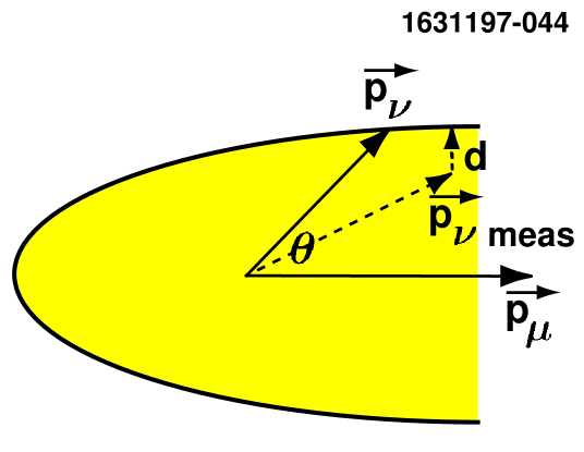
FIG. 1.: The relationship between the muon and neutrino momentum vectors and the constraint surface imposed by the $D_{s}$ invariant mass.

We use Monte Carlo simulation to determine the $\Delta M$ signal shape (Eq. 2) and to estimate our efficiency. Since this analysis involves reconstructing a missing neutrino, we are concerned that the Monte Carlo will not adequately simulate the data. As a check we evaluate the accuracy of our simulation using our $D^{*o}\to\gamma D^{o}$, $D^{o}\to K^{-}\pi^{+}$ sample, where we eliminate the $\pi^{+}$ to simulate the neutrino and treat the $K^{-}$ as a muon.

We start with a $D^{*o}\to\gamma D^{o}$, $D^{o}\to K^{-}\pi^{+}$ Monte Carlo simulation. Fig. 2(a) shows the fully reconstructed mass difference $\Delta M=M(\gamma K\pi)-M(K\pi)$ distribution after a cut on the $K^{-}\pi^{+}$ invariant mass of $\pm$30 MeV around the known $D^{o}$ mass (where the r.m.s resolution is 8 MeV). The kaon is required to have momentum greater than 2.4 GeV/c, which is the same cut as we use on the muon in the $D_{s}^{+}\to\mu^{+}\nu$ channel. In the $\Delta M$ distribution there is a substantial signal but also significant background, so a $\Delta M$ sideband subtraction is performed. We use a bin-by-bin subtraction. The central value of the signal is 142 MeV and the r.m.s. width is 5.5 MeV. The sidebands used are 114-126 MeV and 159-170 MeV. After applying the additional background suppression cuts, described above, we obtain the mass difference distribution $\Delta M=M(\gamma Kp_{miss})-M(Kp_{miss})$ shown in Fig. 3. There is a clear signal peak associated with the photon and it is fitted to an asymmetric Gaussian with low side and high side $\sigma$’s of 15 MeV and 16 MeV, respectively. The small flat component results from replacing the correct photon with another photon.

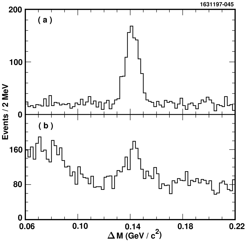
FIG. 2.: The $\Delta M=M(\gamma K^{-}\pi^{+})-M(K^{-}\pi^{+})$ mass difference distributions for fully reconstructed events of $D^{*o}\to\gamma D^{o}$, $D^{o}\to K^{-}\pi^{+}$, after a requirement that the $K^{-}\pi^{+}$ mass be within 2.5 standard deviations of the $D^{o}$ mass. (a) $D^{*o}$ Monte Carlo (b) data.

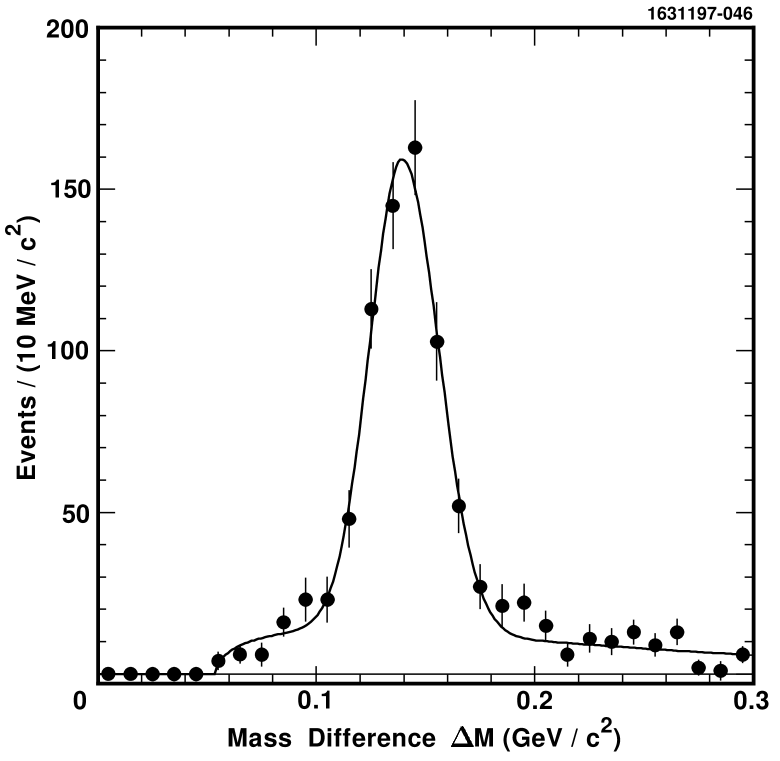
FIG. 3.: The $\Delta M=M(\gamma Kp_{miss})-M(Kp_{miss})$ mass difference distributions for the simulated missing momentum analysis using Monte Carlo of $D^{*o}\to\gamma D^{o}$, $D^{o}\to K^{-}\pi^{+}$. A sideband subtraction to remove background in the initial $D^{*o}$ selection has been applied. The curve and fitting procedure are described in the text.

The partial efficiency for neutrino detection only from Monte Carlo for a fully reconstructed $D^{*o}$ event with both the $D^{*o}$ and its kaon daughter having a momentum greater than 2.4 GeV to appear in the signal peak after neutrino reconstruction is found to be $\epsilon_{\nu}$ = (38.9$\pm$2.6)% [12]. The overall detection efficiency for $D^{*o}\to D^{o}\gamma$, $D^{o}\to K^{+}p_{miss}$ is $(4.8\pm 0.3)\%$ [13].

Next, we repeated the analysis described above for the fully reconstructed $D^{*o}\to\gamma D^{o}$ data sample. The fully reconstructed $\Delta M$ distribution is shown in Fig. 2(b). The $\Delta M$ distribution for the missing neutrino is shown in Fig. 4 where the sideband subtraction again has been performed. The fitting parameters derived from the Monte Carlo signal shape fit the data very well, with a $\chi^{2}$ of 23 for 27 degrees of freedom and a confidence level of 69%. The partial efficiency for neutrino detection oly of (38.5$\pm$3.7)% agrees well with Monte Carlo simulation.

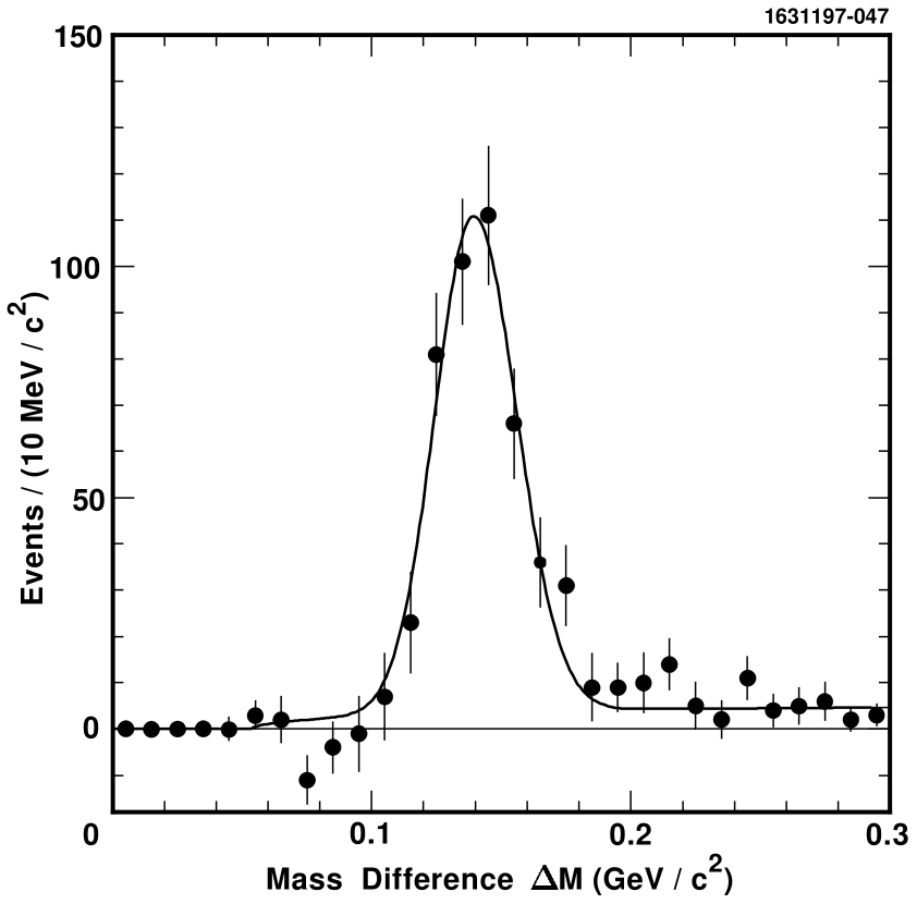
FIG. 4.: The $\Delta M=M(\gamma Kp_{miss})-M(Kp_{miss})$ mass difference distributions for the simulated missing momentum analysis for the $D^{*o}\to\gamma D^{o}$, $D^{o}\to K^{-}\pi^{+}$ real data. A sideband subtraction to remove background in the initial $D^{o}$ selection has been applied. The curve used is from the Monte Carlo signal shape.

In principle the resolution and efficiency for $D_{s}^{*+}\to\gamma D_{s}^{+}$, $D_{s}^{+}\to\mu^{+}\nu$ can be somewhat different from that for the $D^{*o}$ sample described above, because of the different fragmentation with an $s$ quark rather than a $u$ quark. Since our Monte Carlo simulation accurately describes the $D^{*o}\to\gamma D^{o}$, $D^{o}\to K^{-}\pi^{+}$ process, we rely on it for our $D^{*}_{s}$ study. In Fig. 5 we show the $\Delta M=M(\gamma\mu^{+}\nu)-M(\mu^{+}\nu)$ distribution from Monte Carlo simulation. This distribution contains a Gaussian part due to the signal, plus a background which occurs when the correct photon from the $D_{s}^{*}$ decay is replaced with another random photon in the event. We fit the histogram with an asymmetric Gaussian signal shape having low side and high side $\sigma$’s of 15 MeV and 17 MeV, and the function $\sqrt{x-x_{0}}e^{-a(x-x_{0})}$ to parameterize the random photon component, where $x\equiv\Delta M$. The Gaussian signal shape agrees well with the $D^{*o}$ Monte Carlo and data. Using the Gaussian signal part only, the overall efficiency is found to be (4.2$\pm$0.3)%, where the error includes the systematic effect of the efficiency difference between data and Monte Carlo determined by the $D^{*o}$ sample.

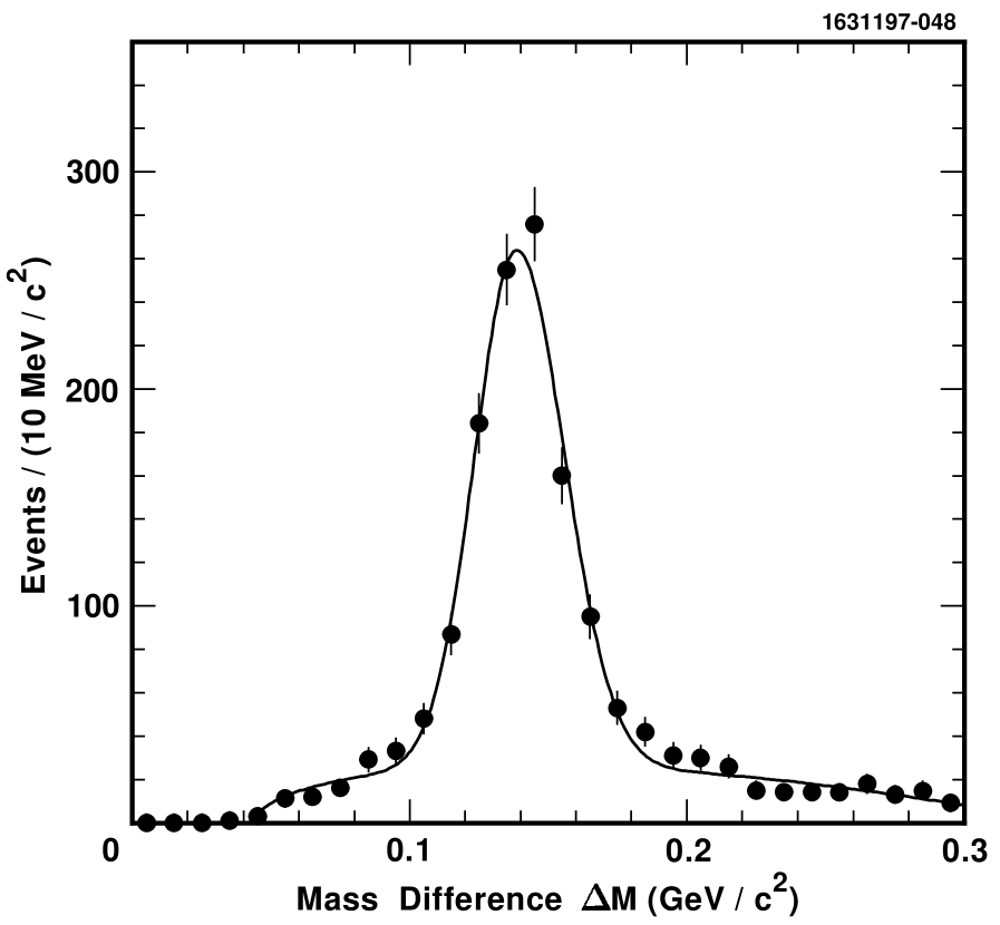
FIG. 5.: The $\Delta M=M(\gamma\mu p_{miss})-M(\mu p_{miss})$ mass difference distributions for the missing momentum analysis for the $D_{s}^{*+}\to\gamma D_{s}^{+}$, $D_{s}^{+}\to\mu^{+}\nu$ Monte Carlo. The curve and fitting procedure are described in the text.

An additional source of background in the $\Delta M$ distribution comes from direct $D_{s}^{+}\to\mu^{+}\nu$ decays which pair with a random photon to form a $D_{s}^{*+}$ candidate. These are in addition to $D_{s}^{*+}$ events where the correct photon is replaced by another photon, as mentioned above. These two contributions are fixed relative to the direct $D_{s}^{*+}\to\gamma D_{s}^{+},D_{s}^{+}\to\mu\nu$ signal using our measurement of $D_{s}^{*+}/D_{s}^{+}$ production ratio above 2.4 GeV of 1.08$\pm$0.13 (see below). Thirdly, there is a small contribution from $D^{+}\to\mu^{+}\nu$ decays combined with a random photon. The shape in $\Delta M$ of all these contributions is modeled using the $D^{*+}\to\pi^{+}D^{o}$ event sample, by combining the $M(Kp_{miss})$ candidates with random photons in the same event, and fitting with the functional form $\sqrt{x-x_{0}}e^{-a(x-x_{0})}$ to parameterize the total random photon component. The distributions in Fig. 5 and the random photon component function are summed using appropriate weights to produce the expected shape for the sum of the $D_{s}^{*+}\to\gamma D^{+}_{s},~{}D_{s}^{+}\to\mu^{+}\nu$ signal plus random photon background shown in Fig. 6.

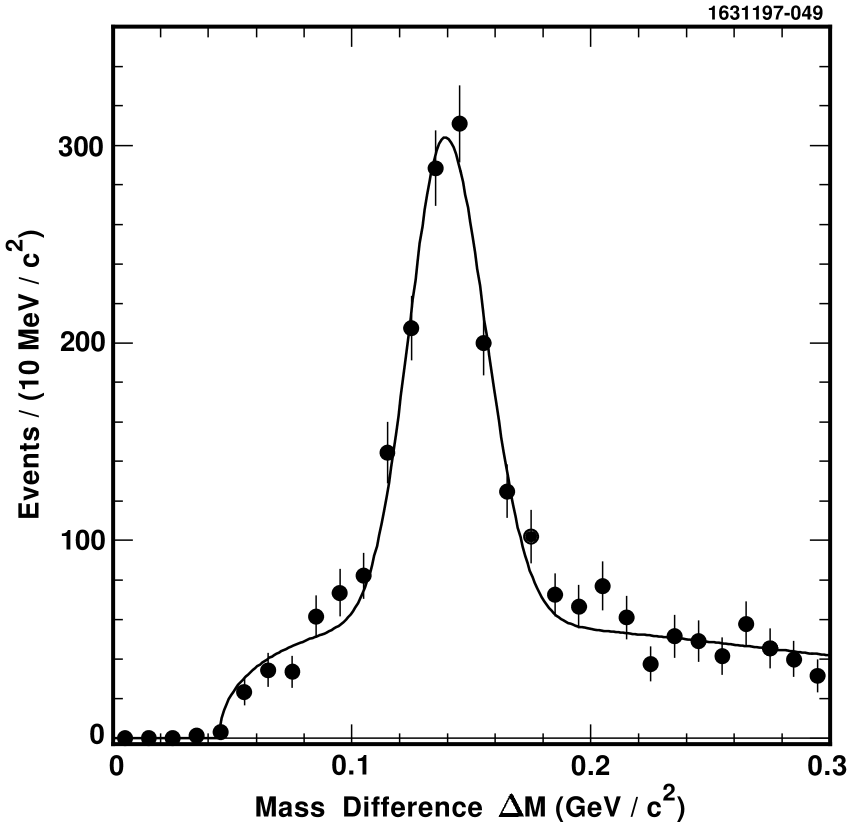
FIG. 6.: The $D_{s}^{*+}\to\gamma D_{s}^{+}$, $D_{s}^{+}\to\mu^{+}\nu$ signal distribution plus random photon background as determined from the signal Monte Carlo simulation combined with the $D^{*+}$ data sample analyzed for the missing $\nu$ as $D^{*o}\to\gamma D^{o}$, $D^{o}\to K^{-}p_{miss}.$ The curve is a fit using the functions described in the text.

E Measurement of the $D_{s}^{+}$ and $D_{s}^{*+}$ Rates

In order to measure the relative rates of $D_{s}^{*}$ and $D_{s}$ production, and the absolute level of $D_{s}$ production above 2.4 GeV/c we use the $D_{s}^{+}\to\phi\pi^{+}$ decay mode. The $\phi$ is searched for in the $K^{+}K^{-}$ decay mode. We require the photon from the $D_{s}^{*+}$ decay to satisfy the same requirements as for the $\mu^{+}\nu$ final state. The detection efficiency for the $\phi\pi^{+}$ decay mode is 22.3%, while for the $D_{s}^{*+}$ the efficiency is 9.4% [14].

Fig. 7(a) shows both the invariant mass of the $\phi\pi^{+}$. In (b), we show $\Delta M=M(\gamma\phi\pi^{+})-M(\phi\pi^{+})$ after requiring that the $\phi\pi^{+}$ mass be within $\pm$24 MeV of the $D_{s}^{+}$ mass.

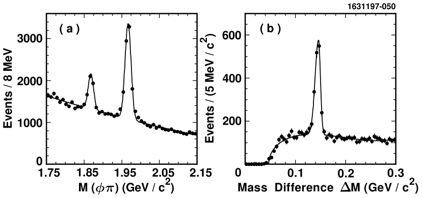
FIG. 7.: (a) The $\phi\pi^{+}$ mass distribution and (b) the $\Delta M=M(\gamma\phi\pi^{+})-M(\phi\pi^{+})$ mass difference distribution with the requirement that $\phi\pi^{+}$ mass is consistent with the known $D_{s}^{+}$ mass. The signal shapes are taken from Monte Carlo simulation. The background shape in (a) is a second order polynominal, while in (b) it is the sum of half-integer polynomials.

Fitting the data to Gaussian signals shapes whose widths are determined by Monte Carlo simulation we find 5728$\pm$123 $D_{s}^{+}\to\phi\pi^{+}$ events and 1256$\pm$54 $D_{s}^{*+}$ events. Taking into account the relative efficiencies we determine that the ratio of $D_{s}^{*+}/D_{s}^{+}$ production is 1.08$\pm$0.13. This number reflects the direct production of a vector charmed-strange meson relative to the direct production of a pseudoscalar charmed-strange meson, above 2.4 GeV/c [15].

III Lepton Fake Background Calculation

Even after strict lepton identification requirements have been applied, significant numbers of hadron fakes still enter our signal region because of the abundance of fast hadron tracks. To properly account for the hadron fake background, we need to measure precisely the effective excess muon to electron fake rate ratio to derive the correct background level. The $D^{*}$ decays provide us with well-tagged kaon and pion samples. In our previous publication, the uncertainty in the fake rate value dominated the systematic errors. One major improvement of the current analysis is the better determination of these rates for muons and electrons from much larger tagged data samples obtained by using new data and adding more channels.

In this analysis, in addition to the decay sequence $D^{*+}\to D^{o}\pi^{+}\to(K^{-}\pi^{+})\pi^{+}$, we also include $D^{*+}\to D^{o}\pi^{+}\to(K^{-}\rho^{+})\pi^{+}$, and $D^{*o}\to D^{o}\pi^{o}\to(K^{-}\pi^{+})\pi^{o}$ to get as many events as possible. $K_{S}\to\pi^{+}\pi^{-}$ samples are also used to determine the pion fake rate and are combined with the $D^{*}$ results to get better statistics. Over 10,000 events were collected with either a $\pi$ or $K$ with momentum greater than 2.4 GeV from the above channels.

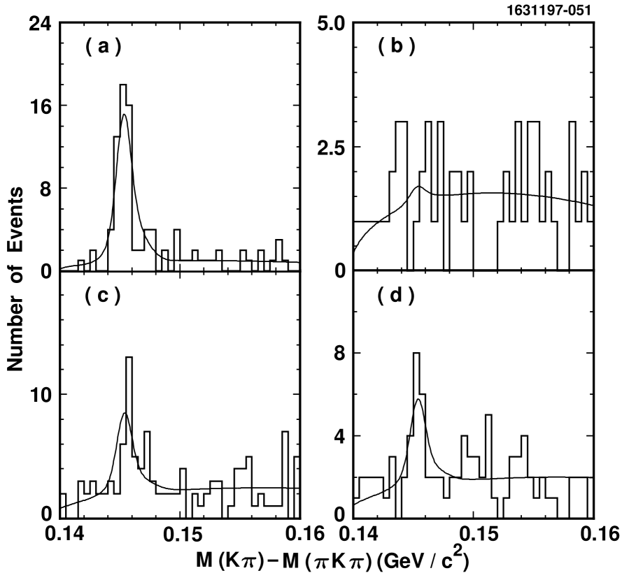
FIG. 8.: $M(\pi K\pi)-M(K\pi)$ mass difference distributions for four cases of hadrons identified as leptons: (a) kaon as muon, (b) kaon as electron, (c) pion as muon, (d) pion as electron. The signal shapes were determined from the distribution of mass difference for fully reconstructed $D^{*+}$ candiates. The area of the Gaussian component and the normalization of the background are allowed to float.

In Fig. 8 we show the $M(\pi^{+}K^{-}\pi^{+})-M(K^{-}\pi^{+})$ mass difference after a cut on $K\pi$ mass consistent with the $D^{o}$ mass for kaons or pions which pass our cuts for muons or electrons The number of events is determined by a fit with a double Gaussian for the signal and half-integer power polynomials for background. Both fitting function shapes are derived from the mass difference distribution without lepton identification suppression. Our extracted fake rates (before decay in flight correction) are listed in Table I. The same reconstruction methods are used to collect kaon and pion samples from the channels $D^{o}\to K^{-}\rho^{+}$, and $D^{*o}\to D^{o}\pi^{o}$ where $D^{o}$ goes to $K^{-}\pi^{+}$ sample. The fake rates are determined by fitting the mass distributions for the amount of signal. The fake rates derived from the different channels are summarized in Table I, and the weighted average fake rates are also shown.

TABLE I.: Fake Rates for P $>$ 2.4 GeV/c

Data Samples	$\#~{}of$	$\#~{}of$	Fake Rates (%)
	$K$	$\pi$	$K/\mu$	$K/e$	$\pi/\mu$	$\pi/e$
$D^{*+}(D^{o}\to K^{-}\pi^{+})$	9404	7461	0.94$\pm$0.11	0.04$\pm$0.05	0.60$\pm$0.12	0.24$\pm$0.06
$D^{*+}(D^{o}\to K^{-}\rho^{+})$	1368	682	1.23$\pm$0.33	0.22$\pm$0.20	0.30$\pm$0.40	0.15$\pm$0.21
$D^{*o}(D^{o}\to K^{-}\pi^{+})$	3174	2048	1.07$\pm$0.21	0.17$\pm$0.10	0.84$\pm$0.35	0.60$\pm$0.31
$K_{S}\to\pi^{+}\pi^{-}$	-	3527	-	-	0.74$\pm$0.15	0.37$\pm$0.10
Total/Average	13964	13718	0.98$\pm$0.08	0.12$\pm$0.05	0.65$\pm$0.08	0.31$\pm$0.06

The contributions to the lepton fake rates from kaon and pion decays in flight are not necessarily included in the above procedure because particles decaying close to the production point may not appear in the $D^{o}$ mass peak. To account for this effect, we used a Monte Carlo study of 200,000 $D^{*+}\to D^{o}\pi^{+}\to(K^{-}\pi^{+})\pi^{+}$ events. After muon identification cuts are applied, the $D^{*+}$ mass difference plot has a peak region used to derive the fake signal and a tail away from the peak, which is due to events in which the kaon decays. We extract a correction factor to the fake rate of 1.18$\pm$0.06 by computing the ratio of the tail area to the peak area. We find no events out of the $D^{*}$ mass difference peak in which the pion has decayed. This is because of the relatively long pion lifetime and because the muon momentum is very close to that of the parent pion.

We determine the hadron induced muon and electron fake background contributions by multiplying the $\Delta M$ distribution of all tracks, excluding leptons, by the effective fakes rates determined above. The fractions of kaon, pions and protons are 67%, 20% and 13% as ascertained from Monte Carlo simulation. The effective Fake rates from protons and anti-protons are small, $\approx$0.1%, and almost equal for muons and electrons.

IV Results

The $\Delta M$ distributions for the muon and electron data and the calculated effective excess of muon fakes over electron fakes are given in Fig. 9(a). The histogram is the result of a $\chi^{2}$ fit of the muon spectrum to the sum of three contributions: the signal distribution evaluated with the $D_{s}^{*+}$ Monte Carlo plus random photon background evaluated with the $D^{*+}$ sample, the scaled electrons, and the excess of muon over electron fakes. Here, the sizes of the electron and fake contributions are fixed and only the signal normalization is allowed to vary.

We remind the reader that the signal consists of two components, whose relative normalization is fixed. These two components are the decay $D_{s}^{*+}\to\gamma D_{s}^{+}$, $D_{s}^{+}\to\mu^{+}\nu$ and the direct decays $D_{s}^{+}\to\mu\nu$ and $D^{+}\to\mu^{+}\nu$. Our measurement of the $D_{s}^{*+}/D_{s}^{+}$ production ratio allows us to constrain the relative normalization. We find a signal of 182$\pm$22 events in the peak which are attributed to the process $D_{s}^{*+}\to\gamma D_{s}^{+}$, $D_{s}^{+}\to\mu^{+}\nu$. We also find 250$\pm$38 events in the flat part of the distribution corresponding to $D_{s}^{+}\to\mu^{+}\nu$ or $D^{+}\to\mu^{+}\nu$ decays coupled with a random photon. The contribution of a real $D^{+}\to\mu^{+}\nu$ decay with random photons is not entirely negligible since the $D^{*+}\to\gamma D^{+}$ branching ratio does not enter. The $D^{+}$ fraction is estimated to be about (18$\pm$8)% relative to the total $D_{s}^{+}\to\mu^{+}\nu$ plus random photon contribution.

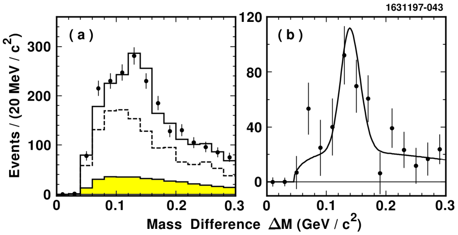
FIG. 9.: (a) The $\Delta M$ mass difference distribution for $D_{s}^{*+}$ candidates for both the muon data (solid points), the electron data (dashed histogram) and the excess of muon fakes over electron fakes (shaded). The histogram is the result of the fit described in the text. (b) The $\Delta M$ mass difference distribution for $D_{s}^{*+}$ candidates with electrons and excess muon fakes subtracted. The curve is a fit to the signal shape described in the text.

To explicitly display the signal, we show, in Fig. 9(b), the $\Delta M$ distribution after the electrons and the fakes are subtracted. The curve is a fit of the data in Fig. 9(a) to the signal shape calculated from the $D_{s}^{*+}$ sample and random photon background calculated from the $D^{*+}$ sample. All of the events in this plot are signal, the background having already been subtracted.

Using the fit result of 182$\pm$22 events, we extract a width for $D_{s}^{+}\to\mu^{+}\nu$ by normalizing to the the efficiency corrected number of fully reconstructed $D_{s}^{*+}\to\gamma D_{s}^{+}$, $D_{s}^{+}\to\phi\pi^{+}$ events, 24740$\pm$1200$\pm$810 [14]. The efficiency for reconstructing the $\phi\pi^{+}$ decay is obtained from Monte Carlo. We find

$${\Gamma(D_{s}^{+}\to\mu^{+}\nu)\over\Gamma(D_{s}^{+}\to\phi\pi^{+})}=0.173\pm 0.023\pm 0.035~{}~{}~{},$$ (8)

where the first error is the statistical error on the measured numbers of $\mu^{+}\nu$ and $\phi\pi^{+}$ events. The second error is the total systematic error of 18%, whose components are summarized in Table II.

TABLE II.: Systematic Errors on Width Ratio (%)

Source of Error	Value	Size of error (%)
Muon fake rate	(0.69$\pm$0.05)%	9
Electron fake rate	(0.21$\pm$0.03)%	7
$\pi/K/p$ fractions (sources of fakes)	67%/20%/13%	7
$\mu$/e normalization	1.01$\pm$0.03	9
Detection efficiency	(4.2$\pm$0.3)%	7
$D_{s}^{*+}/D_{s}^{+}$ production ratio	1.08$\pm$0.13	8
$\phi\pi^{+}$ normalization	24740$\pm$1200$\pm$810	3
Total systematic error		20

The errors that arise from the relative muon to electron normalization, the muon fake rate, the electron fake rate, and the $D_{s}^{*+}/D_{s}^{+}$ production ratio, are estimated by fitting the data with each parameter changed by $\pm$ 1$\sigma$. The error on the relative fractions of pions, kaons and protons entering into the fake rate calculation is computed by changing the fractions to 70%, 20% and 10%, respectively. We judge this to be the outer limit at 90% confidence level of the change possible in these ratios. This, in turn, changes the excess muon to electron to fake rate by 12% leading to a 7% change in the yield. A systematic error of $\pm$3% for the detection efficiency of the normalization mode $\phi\pi^{+}$ is also included.

The radiative decay rates for $D_{s}^{+}\to\ell^{+}\nu\gamma$ and $B^{+}\to\ell^{+}\nu\gamma$ have been considered by Burdman, Goldman and Wyler [23]. They predict that

$${\Gamma(D_{s}^{+}\to\mu^{+}\nu\gamma)\over\Gamma(D_{s}^{+}\to\mu^{+}\nu)}=(1-10)\times 10^{-2}\mu^{2}_{V}{\rm~{}GeV}^{2},$$ (9)

where $\mu^{2}_{V}$ is a vector coupling constant which has a value of approximately 0.1 for the $D_{s}^{+}$ meson. While the radiative decay rate for $B^{+}$ is comparable to the non-radiative rate, the radiative decay rate for $D_{s}^{+}$ is estimated to be between 0.1% and 1% of the non-radiative rate. Furthermore, they also predict that the radiative muon and electron rates are equal, so our electron subtraction would remove any residual effect.

V Conclusions

We have measured the ratio of decay widths

$$\Gamma(D_{s}^{+}\to\mu^{+}\nu)/\Gamma(D_{s}^{+}\to\phi\pi^{+})=0.173\pm 0.023\pm 0.035~{}~{}~{}.$$ (10)

To extract the decay constant $f_{D_{s}}$ we need to known the partial width for the $D_{s}^{+}\to\phi\pi^{+}$ decay. The total $D_{s}^{+}$ width is well known because of precise lifetime measurements [3], but the absolute $\phi\pi^{+}$ branching ratio has a large error. Using the latest PDG average value ${\cal B}(D_{s}^{+}\to\phi\pi^{+})$ of (3.6$\pm$0.9)%, and $\tau_{Ds}=(4.67\pm 0.17)\times 10^{-13}$s, we find

$$f_{D_{s}}=(280\pm 19\pm 28\pm 34){\rm~{}MeV}~{}~{}~{}.$$ (11)

The first error is statistical, and the second is systematic resulting from our relative width ratio measurement, and the third error reflects the uncertainty in the absolute $D_{s}^{+}\to\phi\pi^{+}$ branching ratio. This result supersedes our previous one, using a data sample that includes the one used in the previous analysis. The reduction in the central value is primarily due to the better measurement of the lepton fake rates that lowered the pion/electron fake rate.

For comparison, we list in Table III the old CLEO result and published results from other experiments that used the $D_{s}^{+}\to\mu^{+}\nu$ decay to measure $f_{D_{s}}$. We have changed the values of $f_{D_{s}}$ according to the new PDG $D_{s}$ decay branching fractions for the normalization modes, and have corrected the old CLEO result by using the new fake rates determined in this analysis [5]. The lowering of the central value of the old CLEO result is mostly due to the change in the fake rate determination, which is now much more precise.

TABLE III.: Current Experimental Results on $f_{D_{s}}$ Using $D_{s}^{+}\to\mu^{+}\nu$

Collaboration	Observed	Published $f_{D_{s}}$	Corrected $f_{D_{s}}$
	Events	value (MeV)	value (MeV)
CLEO (old) [4]	39$\pm$8	$344\pm 37\pm 52\pm 42$	$282\pm 30\pm 43\pm 34$
WA75 [5]	6	$232\pm 45\pm 20\pm 48$	$238\pm 47\pm 21\pm 48$
BES [6]	3	$430^{+150}_{-130}\pm 40$	Same
E653 [7]	$23.2\pm 6.0^{+1.0}_{-0.9}$	$194\pm 35\pm 20\pm 14$	$190\pm 34\pm 20\pm 26$
CLEO (this work)	182$\pm$22	-	$280\pm 19\pm 28\pm 34$

In addition, there are new results using the $D_{s}^{+}\to\tau^{+}\nu$ decay from the L3 collaboration [16] of $309\pm 58\pm 33\pm 38$ MeV, and $330\pm 95$ from the DELPHI collaboration [17]. Our new measurement gives the most accurate of $f_{D_{s}}$.

Theoretical predictions of $f_{D_{s}}$ have been made using many methods. Recent lattice gauge calculations [18] give central values of 199 to 221 MeV with quoted errors in the $\pm$40 MeV range. Other theoretical estimates use potential models whose values [19] range from 210 to 356 MeV, and QCD sum rule estimates [20] that are between 200 and 290 MeV. Predictions for $f_{D_{s}}$ have also been made by combining theory with experimental input. Assuming factorization for $\overline{B}\to D^{*}D_{s}^{-}$ decays combined with measured branching ratios, gives a value of $f_{D_{s}}$ range of about 280 MeV with an error of about 60 MeV[21]. Use of experimental data on isospin mass splittings in the $D^{*}$ and $D$ system gives a value for $f_{D}$ of 290 MeV [22]. ($f_{D_{s}}$ is thought to be 10% to 20% higher than $f_{D}$).

ACKNOWLEDGMENTS

We thank Franz Muheim for his creative efforts in the original analysis, and his continuing helpful comments. We gratefully acknowledge the effort of the CESR staff in providing us with excellent luminosity and running conditions. We thank J. Cumalat and W. Johns for interesting discussions. J.P. Alexander, J.R. Patterson, and I.P.J. Shipsey thank the NYI program of the NSF, M. Selen thanks the PFF program of the NSF, G. Eigen thanks the Heisenberg Foundation, K.K. Gan, M. Selen, H.N. Nelson, T. Skwarnicki, and H. Yamamoto thank the OJI program of DOE, J.R. Patterson, K. Honscheid, M. Selen and V. Sharma thank the A.P. Sloan Foundation, M. Selen thanks Research Corporation, and S. von Dombrowski thanks the Swiss National Science Foundation for support. This work was supported by the National Science Foundation, the U.S. Department of Energy, and the Natural Sciences and Engineering Research Council of Canada.

REFERENCES

- [1] J. L. Rosner, in Particles and Fields 3, Proceed. of the 1988 Banff Summer Inst., Banff, Alberta, Canada, ed. by A. N. Kamal and F. C. Khanna, World Scientific, Singapore, 1989, 395.
- [2] Whenever a specific reaction or final state is mentioned, consideration of the charge conjugate reaction or final state is also implied.
- [3] R.M. Barnett et al., (Particle Data Group), Phys. Rev. D 54, 1 (1996).
- [4] D. Acosta et al., Phys. Rev. D49, 5690 (1994).
- [5] S. Aoki et al., Progress of Theoretical Physics 89, 131 (1993). The WA75 value was based on the 1992 PDG value of ( and (. We scale the WA75 result to be MeV using updated PDG [3] values of ( and ( which we use for (, after reducing the value by 3% to account for the smaller muon phase space.
- [6] J. Z. Bai et al., Phys. Rev. Lett. 74, 4599 (1995).
- [7] K. Kodama et al., Phys. Lett. B382 299 (1996).
- [8] Y. Kubota et al., (CLEO Collaboration), Nucl. Instrum. Methods Phys. Res., Sec. A 320, 66 (1992).
- [9] M. S. Alam et al. (CLEO Collaboration), “The Observation of the Radiative Decay ,” CONF 96-7, ICHEP-96 PA01-80 (1996).
- [10] D. Atwood and W. Marciano, Phys. Rev. D41, 1736 (1990).
- [11] To use our , events here, we eliminate the measurements of the fast from the decay from both the tracking chambers and calorimeter to simulate the neutrino, and call the a muon.
- [12] The event sample used is the fully reconstructed sample of events, , , with the required to have momentum above 2.4 GeV/c.
- [13] To compare with the efficiency in the channel, the muon identification effiency of 0.85 must be taken into account, yielding an overall efficiency of 4.1%.
- [14] The efficiencies quoted here are both for momenta above 2.4 GeV/c. To calculate the , yield above 2.4 GeV/c momentum, we remove the cut on the momentum and impose a cut on the momentum.
- [15] The CLEO Collaboration is preparing a publication on the measurement of the vector/pseudoscalar ratio in charmed-strange mesons.
- [16] M. Acciarri et al. (L3 Collaboration), Phys. Lett. B 396, 327 (1997).
- [17] F. Parodi et al. (DELPHI Collaboration), “Measurement of the Branching Fraction ,” DELPHI 97-105 CONF 87, submitted to HEP’97 Conference Jerusalem, August 1997, paper 455.
- [18] See C. Bernard,“Lattice Calculations of Decay Constants,” review talk presented at the Seventh International Symposium on Heavy Flavor Physics, Santa Barbara, July 7-11, 1997, hep-ph/9709460, and references cited therein; A. X. El-Khadra et al., “ and Meson Decay Constants in Lattice QCD,” hep-ph/9711426 (1997).
- [19] H. Krasemann, Phys. Lett. B 96, 397 (1980); M. Suzuki, Phys. Lett. B 162, 391 (1985); S. Godfrey and N. Isgur, Phys. Rev. D 32, 189 (1985); S. N. Sinha, Phys. Lett. B 178, 110 (1986); P. Cea et al., Phys. Lett. B 206, 691 (1988); S. Capstick and S. Godfrey, Phys. Rev. D 41, 2856 (1988).
- [20] C. Dominguez and N. Paver, Phys. Lett. B 197, 423 (1987); S. Narison, Phys. Lett. B 198, 104 (1987); L. J. Reinders, Phys. Rev. D 38, 947 (1988); M. A. Shifman, Usp. Fiz. Nauk 151, 193 (1987) [Sov. Phys. Usp. 30, 91 (1987)].
- [21] D. Bortoletto and S. Stone, Phys. Rev. Lett. 65, 2951 (1990); J. L. Rosner, Phys. Rev. D 42, 3732 (1990); H. Albrecht et al. (ARGUS Collaboration), Zeit. Phys. C 54, 1 (1992); T. Browder, K. Honscheid and S. Playfer, “A Review of Hadronic and Rare Decays,” in Decays 2nd edition, ed. S. Stone, World Scientific, Singapore, p 158 (1994).
- [22] J. F. Amundson et al., Phys. Rev. D 47, 3059 (1993).
- [23] G. Burdman, T. Goldman and D. Wyler, Phys. Rev. D 51, 111 (1995).