Dijet Cross Sections in Photoproduction at HERA

Dijet cross sections are presented using photoproduction data obtained with the ZEUS detector during 1994. These measurements represent an extension of previous results, as the higher statistics allow cross sections to be measured at higher jet transverse energy ($E_{T}^{jet}$). Jets are identified in the hadronic final state using three different algorithms, and the cross sections compared to complete next-to-leading order QCD calculations. Agreement with these calculations is seen for the pseudorapidity dependence of the direct photon events with $E_{T}^{jet}>6$ GeV and of the resolved photon events with $E_{T}^{jet}>11$ GeV. Calculated cross sections for resolved photon processes with 6 GeV $<E_{T}^{jet}<11$ GeV lie below the data.

J. Breitweg, M. Derrick, D. Krakauer, S. Magill, D. Mikunas, B. Musgrave, J. Repond, R. Stanek, R.L. Talaga, R. Yoshida, H. Zhang
Argonne National Laboratory, Argonne, IL, USA ^p

M.C.K. Mattingly
Andrews University, Berrien Springs, MI, USA

F. Anselmo, P. Antonioli, G. Bari, M. Basile, L. Bellagamba, D. Boscherini, A. Bruni, G. Bruni, G. Cara Romeo, G. Castellini¹, L. Cifarelli², F. Cindolo, A. Contin, M. Corradi, S. De Pasquale, I. Gialas³, P. Giusti, G. Iacobucci, G. Laurenti, G. Levi, A. Margotti, T. Massam, R. Nania, F. Palmonari, A. Pesci, A. Polini, F. Ricci, G. Sartorelli, Y. Zamora Garcia⁴, A. Zichichi
University and INFN Bologna, Bologna, Italy ^f

C. Amelung, A. Bornheim, I. Brock, K. Coböken, J. Crittenden, R. Deffner, M. Eckert, L. Feld⁵, M. Grothe, H. Hartmann, K. Heinloth, L. Heinz, E. Hilger, H.-P. Jakob, U.F. Katz, R. Kerger, E. Paul, M. Pfeiffer, Ch. Rembser⁵, J. Stamm, R. Wedemeyer⁶, H. Wieber
Physikalisches Institut der Universität Bonn, Bonn, Germany ^c

D.S. Bailey, S. Campbell-Robson, W.N. Cottingham, B. Foster, R. Hall-Wilton, M.E. Hayes, G.P. Heath, H.F. Heath, J.D. McFall, D. Piccioni, D.G. Roff, R.J. Tapper
H.H. Wills Physics Laboratory, University of Bristol, Bristol, U.K. ^o

M. Arneodo⁷, R. Ayad, M. Capua, A. Garfagnini, L. Iannotti, M. Schioppa, G. Susinno
Calabria University, Physics Dept.and INFN, Cosenza, Italy ^f

J.Y. Kim, J.H. Lee, I.T. Lim, M.Y. Pac⁸
Chonnam National University, Kwangju, Korea ^h

A. Caldwell⁹, N. Cartiglia, Z. Jing, W. Liu, B. Mellado, J.A. Parsons, S. Ritz¹⁰, S. Sampson, F. Sciulli, P.B. Straub, Q. Zhu
Columbia University, Nevis Labs., Irvington on Hudson, N.Y., USA ^q

P. Borzemski, J. Chwastowski, A. Eskreys, J. Figiel, K. Klimek, M.B. Przybycień, L. Zawiejski
Inst. of Nuclear Physics, Cracow, Poland ^j

L. Adamczyk¹¹, B. Bednarek, M. Bukowy, K. Jeleń, D. Kisielewska, T. Kowalski, M. Przybycień, E. Rulikowska-Zarȩbska, L. Suszycki, J. Zaja̧c
Faculty of Physics and Nuclear Techniques, Academy of Mining and Metallurgy, Cracow, Poland ^j

Z. Duliński, A. Kotański
Jagellonian Univ., Dept. of Physics, Cracow, Poland ^k

G. Abbiendi¹², L.A.T. Bauerdick, U. Behrens, H. Beier, J.K. Bienlein, G. Cases¹³, O. Deppe, K. Desler, G. Drews, U. Fricke, D.J. Gilkinson, C. Glasman, P. Göttlicher, T. Haas, W. Hain, D. Hasell, K.F. Johnson¹⁴, M. Kasemann, W. Koch, U. Kötz, H. Kowalski, J. Labs, L. Lindemann, B. Löhr, M. Löwe¹⁵, O. Mańczak, J. Milewski, T. Monteiro¹⁶, J.S.T. Ng¹⁷, D. Notz, K. Ohrenberg¹⁸, I.H. Park¹⁹, A. Pellegrino, F. Pelucchi, K. Piotrzkowski, M. Roco²⁰, M. Rohde, J. Roldán, J.J. Ryan, A.A. Savin, U. Schneekloth, F. Selonke, B. Surrow, E. Tassi, T. Voß²¹, D. Westphal, G. Wolf, U. Wollmer²², C. Youngman, A.F. Żarnecki, W. Zeuner
Deutsches Elektronen-Synchrotron DESY, Hamburg, Germany

B.D. Burow, H.J. Grabosch, A. Meyer, S. Schlenstedt
DESY-IfH Zeuthen, Zeuthen, Germany

G. Barbagli, E. Gallo, P. Pelfer
University and INFN, Florence, Italy ^f

G. Maccarrone, L. Votano
INFN, Laboratori Nazionali di Frascati, Frascati, Italy ^f

A. Bamberger, S. Eisenhardt, P. Markun, T. Trefzger²³, S. Wölfle
Fakultät für Physik der Universität Freiburg i.Br., Freiburg i.Br., Germany ^c

J.T. Bromley, N.H. Brook, P.J. Bussey, A.T. Doyle, N. Macdonald, D.H. Saxon, L.E. Sinclair, E. Strickland, R. Waugh
Dept. of Physics and Astronomy, University of Glasgow, Glasgow, U.K. ^o

I. Bohnet, N. Gendner, U. Holm, A. Meyer-Larsen, H. Salehi, K. Wick
Hamburg University, I. Institute of Exp. Physics, Hamburg, Germany ^c

L.K. Gladilin²⁴, D. Horstmann, D. Kçira, R. Klanner, E. Lohrmann, G. Poelz, W. Schott²⁵, F. Zetsche
Hamburg University, II. Institute of Exp. Physics, Hamburg, Germany ^c

T.C. Bacon, I. Butterworth, J.E. Cole, G. Howell, B.H.Y. Hung, L. Lamberti²⁶, K.R. Long, D.B. Miller, N. Pavel, A. Prinias²⁷, J.K. Sedgbeer, D. Sideris, R. Walker
Imperial College London, High Energy Nuclear Physics Group, London, U.K. ^o

U. Mallik, S.M. Wang, J.T. Wu
University of Iowa, Physics and Astronomy Dept., Iowa City, USA ^p

P. Cloth, D. Filges
Forschungszentrum Jülich, Institut für Kernphysik, Jülich, Germany

J.I. Fleck⁵, T. Ishii, M. Kuze, I. Suzuki²⁸, K. Tokushuku, S. Yamada, K. Yamauchi, Y. Yamazaki²⁹
Institute of Particle and Nuclear Studies, KEK, Tsukuba, Japan ^g

S.J. Hong, S.B. Lee, S.W. Nam³⁰, S.K. Park
Korea University, Seoul, Korea ^h

F. Barreiro, J.P. Fernández, G. García, R. Graciani, J.M. Hernández, L. Hervás⁵, L. Labarga, M. Martínez, J. del Peso, J. Puga, J. Terrón³¹, J.F. de Trocóniz
Univer. Autónoma Madrid, Depto de Física Teórica, Madrid, Spain ⁿ

F. Corriveau, D.S. Hanna, J. Hartmann, L.W. Hung, W.N. Murray, A. Ochs, M. Riveline, D.G. Stairs, M. St-Laurent, R. Ullmann
McGill University, Dept. of Physics, Montréal, Québec, Canada ${}^{a},$  ^b

T. Tsurugai
Meiji Gakuin University, Faculty of General Education, Yokohama, Japan

V. Bashkirov, B.A. Dolgoshein, A. Stifutkin
Moscow Engineering Physics Institute, Moscow, Russia ^l

G.L. Bashindzhagyan, P.F. Ermolov, Yu.A. Golubkov, L.A. Khein, N.A. Korotkova, I.A. Korzhavina, V.A. Kuzmin, O.Yu. Lukina, A.S. Proskuryakov, L.M. Shcheglova³², A.N. Solomin³², S.A. Zotkin
Moscow State University, Institute of Nuclear Physics, Moscow, Russia ^m

C. Bokel, M. Botje, N. Brümmer, F. Chlebana²⁰, J. Engelen, E. Koffeman, P. Kooijman, A. van Sighem, H. Tiecke, N. Tuning, W. Verkerke, J. Vossebeld, M. Vreeswijk⁵, L. Wiggers, E. de Wolf
NIKHEF and University of Amsterdam, Amsterdam, Netherlands ⁱ

D. Acosta, B. Bylsma, L.S. Durkin, J. Gilmore, C.M. Ginsburg, C.L. Kim, T.Y. Ling, P. Nylander, T.A. Romanowski³³
Ohio State University, Physics Department, Columbus, Ohio, USA ^p

H.E. Blaikley, R.J. Cashmore, A.M. Cooper-Sarkar, R.C.E. Devenish, J.K. Edmonds, J. Große-Knetter³⁴, N. Harnew, C. Nath, V.A. Noyes³⁵, A. Quadt, O. Ruske, J.R. Tickner²⁷, H. Uijterwaal, R. Walczak, D.S. Waters
Department of Physics, University of Oxford, Oxford, U.K. ^o

A. Bertolin, R. Brugnera, R. Carlin, F. Dal Corso, U. Dosselli, S. Limentani, M. Morandin, M. Posocco, L. Stanco, R. Stroili, C. Voci
Dipartimento di Fisica dell’ Università and INFN, Padova, Italy ^f

J. Bulmahn, B.Y. Oh, J.R. Okrasiński, W.S. Toothacker, J.J. Whitmore
Pennsylvania State University, Dept. of Physics, University Park, PA, USA ^q

Y. Iga
Polytechnic University, Sagamihara, Japan ^g

G. D’Agostini, G. Marini, A. Nigro, M. Raso
Dipartimento di Fisica, Univ. ’La Sapienza’ and INFN, Rome, Italy ${}^{f}~{}$

J.C. Hart, N.A. McCubbin, T.P. Shah
Rutherford Appleton Laboratory, Chilton, Didcot, Oxon, U.K. ^o

D. Epperson, C. Heusch, J.T. Rahn, H.F.-W. Sadrozinski, A. Seiden, R. Wichmann, D.C. Williams
University of California, Santa Cruz, CA, USA ^p

O. Schwarzer, A.H. Walenta
Fachbereich Physik der Universität-Gesamthochschule Siegen, Germany ^c

H. Abramowicz³⁶, G. Briskin, S. Dagan³⁶, S. Kananov³⁶, A. Levy³⁶
Raymond and Beverly Sackler Faculty of Exact Sciences, School of Physics, Tel-Aviv University,
Tel-Aviv, Israel ^e

T. Abe, T. Fusayasu, M. Inuzuka, K. Nagano, K. Umemori, T. Yamashita
Department of Physics, University of Tokyo, Tokyo, Japan ^g

R. Hamatsu, T. Hirose, K. Homma³⁷, S. Kitamura³⁸, T. Matsushita
Tokyo Metropolitan University, Dept. of Physics, Tokyo, Japan ^g

R. Cirio, M. Costa, M.I. Ferrero, S. Maselli, V. Monaco, C. Peroni, M.C. Petrucci, M. Ruspa, R. Sacchi, A. Solano, A. Staiano
Università di Torino, Dipartimento di Fisica Sperimentale and INFN, Torino, Italy ^f

M. Dardo
II Faculty of Sciences, Torino University and INFN - Alessandria, Italy ^f

D.C. Bailey, C.-P. Fagerstroem, R. Galea, G.F. Hartner, K.K. Joo, G.M. Levman, J.F. Martin, R.S. Orr, S. Polenz, A. Sabetfakhri, D. Simmons, R.J. Teuscher⁵
University of Toronto, Dept. of Physics, Toronto, Ont., Canada ^a

J.M. Butterworth, C.D. Catterall, T.W. Jones, J.B. Lane, R.L. Saunders, M.R. Sutton, M. Wing
University College London, Physics and Astronomy Dept., London, U.K. ^o

J. Ciborowski, G. Grzelak³⁹, M. Kasprzak, K. Muchorowski⁴⁰, R.J. Nowak, J.M. Pawlak, R. Pawlak, T. Tymieniecka, A.K. Wróblewski, J.A. Zakrzewski
Warsaw University, Institute of Experimental Physics, Warsaw, Poland ^j

M. Adamus
Institute for Nuclear Studies, Warsaw, Poland ^j

C. Coldewey, Y. Eisenberg³⁶, D. Hochman, U. Karshon³⁶
Weizmann Institute, Department of Particle Physics, Rehovot, Israel ^d

W.F. Badgett, D. Chapin, R. Cross, S. Dasu, C. Foudas, R.J. Loveless, S. Mattingly, D.D. Reeder, W.H. Smith, A. Vaiciulis, M. Wodarczyk
University of Wisconsin, Dept. of Physics, Madison, WI, USA ^p

A. Deshpande, S. Dhawan, V.W. Hughes
Yale University, Department of Physics, New Haven, CT, USA ^p

S. Bhadra, W.R. Frisken, M. Khakzad, W.B. Schmidke
York University, Dept. of Physics, North York, Ont., Canada ^a

¹ also at IROE Florence, Italy
² now at Univ. of Salerno and INFN Napoli, Italy
³ now at Univ. of Crete, Greece
⁴ supported by Worldlab, Lausanne, Switzerland
⁵ now at CERN
⁶ retired
⁷ also at University of Torino and Alexander von Humboldt Fellow at DESY
⁸ now at Dongshin University, Naju, Korea
⁹ also at DESY
¹⁰ Alfred P. Sloan Foundation Fellow
¹¹ supported by the Polish State Committee for Scientific Research, grant No. 2P03B14912
¹² supported by an EC fellowship number ERBFMBICT 950172
¹³ now at SAP A.G., Walldorf
¹⁴ visitor from Florida State University
¹⁵ now at ALCATEL Mobile Communication GmbH, Stuttgart
¹⁶ supported by European Community Program PRAXIS XXI
¹⁷ now at DESY-Group FDET
¹⁸ now at DESY Computer Center
¹⁹ visitor from Kyungpook National University, Taegu, Korea, partially supported by DESY
²⁰ now at Fermi National Accelerator Laboratory (FNAL), Batavia, IL, USA
²¹ now at NORCOM Infosystems, Hamburg
²² now at Oxford University, supported by DAAD fellowship HSP II-AUFE III
²³ now at ATLAS Collaboration, Univ. of Munich
²⁴ on leave from MSU, supported by the GIF, contract I-0444-176.07/95
²⁵ now a self-employed consultant
²⁶ supported by an EC fellowship
²⁷ PPARC Post-doctoral Fellow
²⁸ now at Osaka Univ., Osaka, Japan
²⁹ supported by JSPS Postdoctoral Fellowships for Research Abroad
³⁰ now at Wayne State University, Detroit
³¹ partially supported by Comunidad Autonoma Madrid
³² partially supported by the Foundation for German-Russian Collaboration DFG-RFBR
    (grant no. 436 RUS 113/248/3 and no. 436 RUS 113/248/2)
³³ now at Department of Energy, Washington
³⁴ supported by the Feodor Lynen Program of the Alexander von Humboldt foundation
³⁵ Glasstone Fellow
³⁶ supported by a MINERVA Fellowship
³⁷ now at ICEPP, Univ. of Tokyo, Tokyo, Japan
³⁸ present address: Tokyo Metropolitan College of Allied Medical Sciences, Tokyo 116, Japan
³⁹ supported by the Polish State Committee for Scientific Research, grant No. 2P03B09308
⁴⁰ supported by the Polish State Committee for Scientific Research, grant No. 2P03B09208

a	supported by the Natural Sciences and Engineering Research Council of Canada (NSERC)
b	supported by the FCAR of Québec, Canada
c	supported by the German Federal Ministry for Education and Science, Research and Technology (BMBF), under contract numbers 057BN19P, 057FR19P, 057HH19P, 057HH29P, 057SI75I
d	supported by the MINERVA Gesellschaft für Forschung GmbH, the German Israeli Foundation, and the U.S.-Israel Binational Science Foundation
e	supported by the German Israeli Foundation, and by the Israel Science Foundation
f	supported by the Italian National Institute for Nuclear Physics (INFN)
g	supported by the Japanese Ministry of Education, Science and Culture (the Monbusho) and its grants for Scientific Research
h	supported by the Korean Ministry of Education and Korea Science and Engineering Foundation
i	supported by the Netherlands Foundation for Research on Matter (FOM)
j	supported by the Polish State Committee for Scientific Research, grant No. 115/E-343/SPUB/P03/002/97, 2P03B10512, 2P03B10612, 2P03B14212, 2P03B10412
k	supported by the Polish State Committee for Scientific Research (grant No. 2P03B08308) and Foundation for Polish-German Collaboration
l	partially supported by the German Federal Ministry for Education and Science, Research and Technology (BMBF)
m	supported by the Fund for Fundamental Research of Russian Ministry for Science and Education and by the German Federal Ministry for Education and Science, Research and Technology (BMBF)
n	supported by the Spanish Ministry of Education and Science through funds provided by CICYT
o	supported by the Particle Physics and Astronomy Research Council
p	supported by the US Department of Energy
q	supported by the US National Science Foundation

1 Introduction

High energy collisions between photons and protons can produce jets in the final state. In leading order quantum chromodynamics (LO QCD), two types of processes lead to the photoproduction of jets. In direct processes the photon participates in the hard scatter via either boson-gluon fusion or QCD Compton scattering. In resolved processes the photon acts as a source of quarks and gluons, and only a fraction of its momentum participates in the hard scatter. This separation between direct and resolved photoproduction is only well defined in this way at leading order. To make a measurement which can be compared to calculations at any order, the variable $x_{\gamma}^{OBS}$ is used to separate these two types of event [1]. The variable $x_{\gamma}^{OBS}$ is the fraction of the photon’s momentum contributing to the production of the two highest transverse energy ($E_{T}^{jet}$) jets. It is defined for the photoproduction of jets in positron-proton scattering as:

$$x_{\gamma}^{OBS}=\frac{E_{T}^{jet1}e^{-\eta^{jet1}}+E_{T}^{jet2}e^{-\eta^{jet2}}}{2yE_{e}}$$ (1)

where $E_{e}$ is the initial positron energy and $\eta^{jet}$ is the jet pseudorapidity. The inelasticity $y$ is defined in the ZEUS frame as $y=1-\frac{E^{\prime}_{e}}{2E_{e}}(1-\cos{\theta^{\prime}_{e}})$ where $E^{\prime}_{e}$ and $\theta^{\prime}_{e}$ are the energy and polar angle of the outgoing positron. In a leading order calculation, direct processes have $x_{\gamma}^{OBS}=1$ since all the photon’s momentum participates in the production of the high transverse energy jets, while resolved processes have $x_{\gamma}^{OBS}<1$ since part of the photon’s momentum goes into the photon remnant. Throughout the following, in both the data and the calculations, direct and resolved samples are defined in terms of a cut on $x_{\gamma}^{OBS}$ rather than in terms of the LO diagrams. In a recent analysis by the H1 collaboration, a similar variable was used to determine an effective parton distribution in the photon [2].

In a previous analysis [1] dijet cross sections were measured using 1993 ZEUS data in the kinematic regime where the difference between the pseudorapidities of the two jets is small ($|\Delta\eta|=|\eta^{jet1}-\eta^{jet2}|<0.5$). This condition constrains $\theta^{\ast}$, the angle between the jet-jet axis and the beam axis in the dijet centre of mass system, to be close to $90^{o}$. The cross section as a function of $\bar{\eta}=(\eta^{jet1}+\eta^{jet2})/2$ then has maximal sensitivity to the parton distributions in both the photon and proton [3]. In [1], the comparison between data and Monte Carlo (MC) simulations based on the LO direct and resolved processes showed that the jet profiles, as described by the transverse energy flow around the jet axis, are poorly reproduced for jets with low $E_{T}^{jet}$ produced in the forward (proton) direction. In the present analysis a comparison will be made with MC simulations which include multiparton interactions, and an improved description of the data is obtained.

To compare data and theoretical cross sections based on next-to-leading order (NLO) QCD calculations, it is essential that similar jet definitions be employed for both the measurement and calculations. The dijet cross sections as a function of $E_{T}^{jet}$ and $\bar{\eta}$, for low and high $x_{\gamma}^{OBS}$, are measured in the hadronic final state using various jet definitions, including the $k_{T}$ algorithm. The resulting cross sections are compared to NLO QCD calculations at the parton level. The uncertainties due to hadronization effects are not yet theoretically estimated and are not considered in the comparison. After a brief description of the experimental setup, a discussion of the issues involved in the various jet definitions in both theory and experiment is presented, followed by our results and conclusions.

2 Experimental Setup

In 1994 HERA provided 27.5 GeV positrons and 820 GeV protons colliding in 153 bunches. Additional unpaired positron and proton bunches circulated to allow monitoring of the background from beam-gas interactions. Events from empty beam crossings (that is bunches containing neither positrons nor protons) were used to estimate the background from cosmic rays. The total integrated luminosity used in this analysis is $2.70$ pb^-1 with an uncertainty of $\pm$1.5%.

Details of the ZEUS detector have been described elsewhere [4]. The primary components used in this analysis are the central tracking system and the calorimeter. The central tracking system consists of a vertex detector [5] and a central tracking detector [6] enclosed in a 1.43 T solenoidal magnetic field. The uranium and scintillator calorimeter [7] covers 99.7% of the total solid angle and is subdivided into three parts: forward (FCAL) covering $4.3>\eta>1.1$, barrel (BCAL) covering the central region $1.1>\eta>-0.75$ and rear (RCAL) covering the backward region $-0.75>\eta>-3.8$, for a collision at the nominal interaction point. Each calorimeter part consists of an electromagnetic section followed by an hadronic section. The cells of these sections have inner face sizes of $5\times 20$ cm² ($10\times 20$ cm² in the rear calorimeter) and $20\times 20$ cm², respectively. A lead and scintillator calorimeter is used to measure the luminosity via the the detection of photons from the positron-proton bremsstrahlung process. This calorimeter is installed 107 m along the HERA tunnel from the interaction point in the positron direction and subtends a small angle at the interaction vertex [8]. A fraction of the positrons scattered through small angles are detected in a similar lead and scintillator calorimeter positioned at $Z=-35$ m.

3 Jet Algorithms

Most of the previous measurements of jet cross sections at hadron-hadron colliders and in photoproduction at HERA have used some variation of a cone-based jet algorithm. In these algorithms, according to the standardisation of cone jet algorithms at the Snowmass meeting in 1990 [9], jets consist of calorimeter cells (or, in a theoretical description, partons) $i$ with a distance

$$R_{i}=\sqrt{(\eta_{i}-\eta^{jet})^{2}+(\phi_{i}-\phi^{jet})^{2}}\leq R$$ (2)

from the jet centre. Here $\phi_{i}$ and $\eta_{i}$ are the azimuthal angle and pseudorapidity of the cell (or parton), and $R$ is the jet cone radius. In this analysis, the geometric centre of the cell is used to define the position. The parameters for the jet are calculated as:

$$E_{T}^{jet} = \sum_{i}E_{T_{i}}$$

$$\eta^{jet} = \frac{1}{E_{T}^{jet}}\sum_{i}E_{T_{i}}\eta_{i}$$ (3)

$$\phi^{jet} = \frac{1}{E_{T}^{jet}{}}\sum_{i}E_{T_{i}}\phi_{i}$$

in which the sums run over all calorimeter cells (or partons) belonging to the jet. Different approaches are possible to the choice of the ‘seed’ with which to begin jet finding, and to how and when overlapping jets are merged. The approach is not fixed by the Snowmass convention. We use two different cone algorithms to determine dijet cross sections in photoproduction. The jet cone radius $R=1$ is chosen for both algorithms. We also use a cluster algorithm, which does not suffer from these ambiguities. A further advantage of the cluster algorithm is that it is infrared safe to all orders, which is not always the case for cone algorithms [10]. In the following the three algorithms will be described in detail considering as an example the case of calorimeter cells. Identical algorithms are used in this analysis to define jets in the hadronic final state starting from the final state particles.

In the first cone algorithm (EUCELL) a window in the $\eta-\phi$ space of the calorimeter cells is moved around to find those positions where the $E_{T}$ in the window is $>1$ GeV to use as seeds. The jet quantities are initially calculated using the cells in a cone centred on the seed. Equations (2) and (3) are then applied to choose the cells belonging to the jets and to update the jet quantities in an iterative procedure until a stable jet is found. Only the highest transverse energy jet is accepted, the cells within the jet are removed, and the whole process is repeated. In this way EUCELL produces no overlapping jets.

The second cone algorithm (PUCELL) was adapted from the algorithm used by CDF [11] and determines seeds by finding the single calorimeter cell of highest transverse energy and placing a cone around it. All the cells within the selected cone are assigned to this seed and excluded from the search for further seeds, which is then continued. The jet quantities are initially calculated using the cells in the seed and equations (2) and (3) are then applied iteratively as for EUCELL until a stable jet is found. At this stage all jets are provisionally accepted. Thus it may happen that two stable jets overlap. If the overlapping transverse energy amounts to more than 75% of the smallest jet, they are merged, otherwise the overlapping energy is split such that cells are associated with the closest jet.

In the cluster algorithm KTCLUS [12, 13] the quantity

$$d_{i,j}=\left((\eta_{i}-\eta_{j})^{2}+(\phi_{i}-\phi_{j})^{2}\right){\rm min}(E_{T_{i}},E_{T_{j}})^{2}$$ (4)

is calculated for each pair of objects (where the initial objects are the calorimeter cells), and for each individual object:

$$d_{i}=E^{2}_{T_{i}}.$$ (5)

If, of all the numbers [$d_{i,j},d_{i}$], $d_{k,l}$ is the smallest then objects $k$ and $l$ are combined into a single new object. If however $d_{k}$ is the smallest, then object $k$ is a jet and is removed from the sample. This is repeated until all objects are assigned to jets. As with the cone algorithms, eq. (3) is used to determine the parameters of the jets. It is also used to determine the parameters of the intermediate objects.

Equations (2) and (3) imply that in a NLO calculation, two partons must be a distance

$$R_{ij}=\sqrt{(\eta_{i}-\eta_{j})^{2}+(\phi_{i}-\phi_{j})^{2}}\leq\frac{E_{T_{i}}+E_{T_{j}}}{\max(E_{T_{i}},E_{T_{j}})}R$$ (6)

from each other to be combined, where $E_{T_{k}}$ is the transverse energy of parton $k$. This implies that if two partons have approximately equal transverse energy they may be separated from each other by as much as $2R$ and still satisfy eq.(2). However, as parton $j$ does not then lie inside a cone of radius $R$ around parton $i$ and vice versa, one might with some justification also count the two partons separately. If one wishes to compare theory with measurement it is necessary to match the theoretical treatment of such cases to the operation of the jet finding and jet merging criteria used experimentally. This is done by introducing an additional parameter, $R_{\rm sep}$, to the theory to restrict the maximum separation between two partons in a single jet [14]. Eq. (6) then becomes

$$R_{ij}\leq\min\left[\frac{E_{T_{i}}+E_{T_{j}}}{\max(E_{T_{i}},E_{T_{j}})}R,R_{\rm sep}\right].$$ (7)

The valid range of $R_{\rm sep}$ is between $1R$ and $2R$. For a NLO three parton final state, it is found that $R_{\rm sep}=(1.5-2.0)\cdot R$ corresponds to EUCELL, $R_{\rm sep}=1\cdot R$ to PUCELL, and $R=R_{\rm sep}=1$ to KTCLUS [15]. In this paper, all three jet definitions will be used for a comparison of the resulting dijet cross sections. An alternative approach would be to treat $R_{\rm sep}$ as a parameter, and tune it in order to take into account possible theoretical uncertainties such as higher order contributions. However, in the present analysis this approach has not been followed and $R_{\rm sep}$ is fixed by the functionality of each jet algorithm.

4 Event Selection

The ZEUS detector uses a three-level trigger system. The first level selects events used in this analysis with a coincidence of a regional or transverse energy sum in the calorimeter, and at least one track from the interaction point measured in the central tracking chamber. At the second level, at least 8 GeV total transverse energy, excluding the eight calorimeter towers immediately surrounding the forward beampipe, is required, and cuts on calorimeter energies and timing are used to suppress events caused by interactions between the proton beam and residual gas in the beam pipe [16]. At the third level, a cone algorithm uses the calorimeter cell energies and positions to identify jets. Events are required to have at least two jets, each of which has $E_{T}^{TLTJet}>3.5$ GeV and $\eta^{TLTJet}<2.0$ or $E_{T}^{TLTJet}>4.0$ GeV and $2.0<\eta^{TLTJet}<2.5$. Additional tracking cuts were made to reject proton beam-gas interactions and cosmic ray events.

Further cuts are applied offline. Charged current deep inelastic scattering events are rejected by a cut on the missing transverse momentum measured in the calorimeter. To reject remaining beam-gas and cosmic ray background events, tighter cuts using the final $Z-$vertex position, other tracking information and timing information are applied. Two additional cuts are made [17], based upon two different measurements of $y$:

1. Events with a positron candidate in the uranium calorimeter are removed if $y_{e}<0.7$, where $y_{e}$ is the value of $y$ as measured assuming the positron candidate is the scattered positron.

2. A cut is made on the Jacquet-Blondel measurement of $y$ [18], $y_{JB}=\sum_{i}(E_{i}-E_{zi})/2E_{e}$, where $E_{zi}=E_{i}\cos\theta_{i}$, and $E_{i}$ is the energy deposited in the calorimeter cell $i$ which has a polar angle $\theta_{i}$ with respect to the measured $Z$-vertex of the event. The sum runs over all calorimeter cells. For any event where the scattered positron entered the uranium calorimeter and either is not identified or gives $y_{e}$ above $0.7$, the value of $y_{JB}$ will be near to one. Proton beam-gas events will have low values of $y_{JB}$. To further reduce the contamination from both these sources, it is required that $0.15<y_{JB}<0.7$. This range corresponds approximately to the true $y$ range of $0.2<y<0.8$.

These cuts restrict the range of the photon virtuality to less than $\sim 4$ GeV², with a median of around $10^{-3}$ GeV², which excludes deep inelastic scattering (DIS) events.

To select dijet candidates with a particular jet algorithm, the algorithm is applied to the calorimeter cells. In each case, the jet transverse energy measured in the ZEUS detector is corrected as a function of $\eta^{CALJet}$ and $E_{T}^{CALJet}$. The variable $E_{T}^{CALJet}$ is used to denote the transverse energy of a jet before correction for the effects of inactive material. This correction is derived from the MC events described in the next section by comparing the true transverse energy of the jet, found by applying the algorithm to the final state particles, to the (lower) transverse energy measured in the calorimeter simulation, obtaining the average shift between the two transverse energies for each jet algorithm. The average shift in jet energies is around $17\%$ for all three jet algorithms, and varies between $10\%$ and $25\%$ depending upon $\eta^{jet}$. The largest shifts occur at the boundaries between the FCAL and BCAL and between the BCAL and RCAL. No correction was applied to $\eta^{CALJet}$ since, from MC, the average shift in $\eta$ between the particle and detector jets is less than $\pm$0.05 for all $\eta$ values in the range used for the cross section measurements.

The description of the calorimeter response to particles and jets in the MC has been tuned using several methods [19, 20], including (i) the comparison of charged track momenta with calorimeter energy measurements, (ii) comparison of jet and positron variables in DIS events and (iii) the comparison of the measurement of the incident photon energy deduced from the energy of the positron measured in the small-angle positron calorimeter, to that calculated from energy deposits in the uranium calorimeter. The fivefold increase in statistics in 1994 allowed the calorimeter energy scale to be studied in more detail than before, and these studies revealed a $(6\pm 3)\%$ difference between data and MC. This difference was removed in the present analysis ( in the 1993 analysis [1], this difference was not corrected, but the possibility of such a discrepancy was allowed for in the systematic errors). Studies using jet photoproduction events allow us to assign an uncertainty of 5% to the calorimeter response for the jets used in this analysis [20]. Other studies have shown that of this 5% uncertainty, 3% arises from the absolute energy scale of the calorimeter [19].

After the jet energy correction, events are required to have at least two jets with $E_{T}^{jet}~{}\geq~{}6$ GeV, $-1.375<\eta^{jet}<1.875$, and $|\Delta\eta|<0.5$. The MC gives a good description of the $|\Delta\eta|$ distribution around this region. For events with three or more jets, the two highest $E_{T}^{jet}$ jets are used to calculate all jet-related event properties. This procedure is also employed later in all the theoretical and MC predictions shown.

After these cuts about 25000 events remain, of which about 20% have $x_{\gamma}^{OBS}\geq 0.75$ (the exact number depending upon the jet algorithm). Events with a third jet which passes the $E_{T}^{jet}$ and $\eta^{jet}$ cuts comprise about 8% of the final sample. Of all events, 22% have their scattered positrons detected in the small-angle tagger, which is the fraction expected for a sample of photoproduction events [17]. No event from unpaired $e$ or $p$ bunches survives the selection cuts, implying that the non-$ep$ background is negligible. The contamination from events with photon virtualities greater than 4 GeV² is estimated using simulated DIS events. This contribution is much smaller than the statistical errors and is therefore not subtracted from the data.

5 Comparison with Monte Carlo Simulation

In Fig. 1 the $x_{\gamma}^{OBS}$ distribution of the ZEUS data selected using the KTCLUS algorithm with (corrected) $E_{T}^{jet}>6$ GeV, $-1.375<\eta^{jet}<1.875$, and $|\Delta\eta|<0.5$ is shown (black dots). This $x_{\gamma}^{OBS}$ is determined by using the corrected jet energies and corrected $y_{JB}$. The correction to $y_{JB}$ is determined using MC generated events, by comparing $y_{JB}$ to the true $y$, as a function of the $x_{\gamma}^{OBS}$ calculated using uncorrected variables. The peak at high $x_{\gamma}^{OBS}$ due to direct photon processes and the rise at low $x_{\gamma}^{OBS}$ due to resolved photon processes are both clearly visible. The sharp fall off for $x_{\gamma}^{OBS}<0.1$ is a result of the $E_{T}^{jet}$ and $\eta^{jet}$ kinematic cuts.

The data are compared to the results of two LO QCD-based MC simulation programs, HERWIG58 [21] (solid line) and PYTHIA57 [22] (dashed line). All the MC events have been passed through a detailed simulation of the ZEUS detector and through the same jet energy correction procedure as was applied to the data. The GRV [23] parton distributions are used for the photon and the MRSA [24] parton distributions are used for the proton. The simulation programs are based on LO QCD calculations for the hard scatter and include parton showering and hadronisation effects. The minimum transverse momentum of the partonic hard scatter ($\hat{p}_{T}^{\rm min}$) is set to 2.5 GeV in both HERWIG and PYTHIA. For both programs the direct and resolved photon processes are generated separately.

In the case of the resolved processes multiparton interactions (MI) are included [25, 26] as an attempt to simulate the energy from additional softer scatters (‘underlying event’), in both the dashed PYTHIA curve and the solid HERWIG curve. This has been shown to improve the simulation of the energy flow around the jet axis [27].

In order to obtain the best agreement with the data the normalisations of the two processes were determined by allowing them to vary independently and fitting to the uncorrected $x_{\gamma}^{OBS}$ distribution. As a result, the cross section from HERWIG for resolved processes was scaled by 1.2 with respect to the direct. The ratio of direct and resolved contributions using this scaled cross section was then 0.12, to be compared with 0.15 when using the unscaled cross sections within HERWIG. For PYTHIA the equivalent scale factor for the resolved cross section, and the ratio of direct and resolved, were found to be the same as for HERWIG within the precision quoted here.

The dotted line shows the distribution for HERWIG without MI. For the MI, models based upon the independent statistical replication of scatters (eikonal models) are used which allow the generation of additional independent partonic scatters (with transverse momenta above $\hat{p}_{T}^{\rm min}$ = 2.5 GeV for HERWIG and 1.4 GeV for PYTHIA) in resolved photon events. For HERWIG the average number of scatters for events generated with these parameters is 1.05 and for PYTHIA it is 1.66. One effect of MI is to increase the number of events at low $x_{\gamma}^{OBS}$. However, even after the inclusion of MI with these parameters, the data still lie above the simulation at low $x_{\gamma}^{OBS}$.

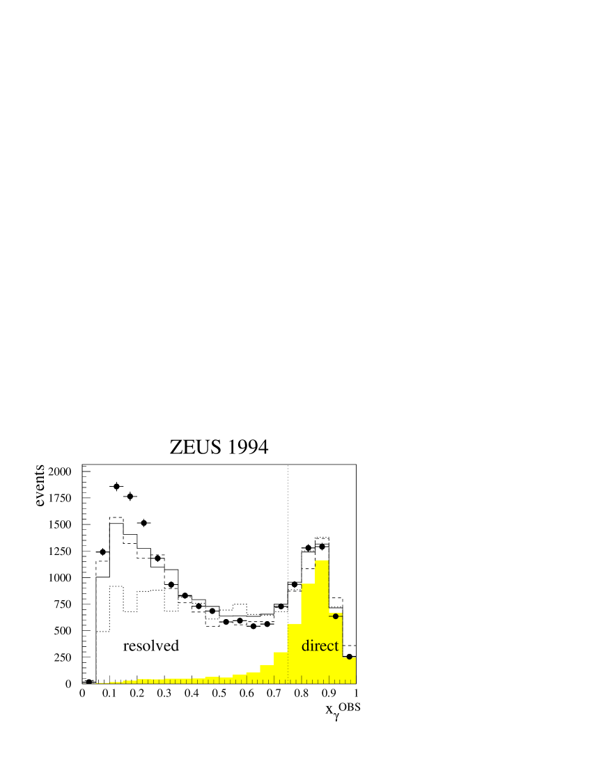
Figure 1: $x_{\gamma}^{OBS}$ distribution for KTCLUS jets with $E_{T}^{jet}>6$ GeV, $-1.375<\eta^{jet}<1.875$ and $|\Delta\eta|<0.5$, where $x_{\gamma}^{OBS}$ is calculated using corrected variables. The ZEUS 1994 data (black dots) are compared to the results of the HERWIG with MI (solid line) and without (dotted line) and PYTHIA with MI (dashed line) event generators after full detector simulation and scaling of MC cross sections (see text). The HERWIG cross section for resolved processes has been scaled by a factor of 1.2 with respect to the direct. The equivalent scaling for PYTHIA is the same. Only statistical errors are shown and in some cases are smaller than the black dots. The shaded area represents the direct process HERWIG MC events.

The uncorrected transverse energy flow around the jets is shown in Fig. 2, for events in various bins of $E_{T}^{CALJet}$ and $\eta^{CALJet}$ for KTCLUS jets, and is compared to the distributions from the HERWIG MC both with and without MI after full simulation of the detector. The jet profiles are described reasonably well by the MC with MI for most of the kinematic range, although there is still a tendency for MC jets to have too much energy inside the central region and too little energy outside this region, particularly for low $E_{T}$ jets in the forward region. This tendency is significantly stronger for MC samples which do not include multiparton interactions. However, we do not rule out the possibility that other models for the underlying event, or different MI parameters not investigated here, may provide a similar or better description of the data.

Figure 2: Uncorrected transverse energy flow $(1/N)dE_{T}/d\delta\eta$ around the jet axis, for cells within one radian in $\phi$ of the jet axis, for KTCLUS jets binned in $E_{T}^{CALJet}$ and $\eta^{CALJet}$ (black dots), where $\delta\eta=\eta^{CELL}-\eta^{CALjet}$. The HERWIG MC with (solid line) and without (dashed line) multiparton interactions are shown for comparison. Only statistical errors are shown.

6 Resolution and Systematics

The resolution of the kinematic variables has been studied by comparing, in the MC simulation, jets reconstructed from final state particles (hadron jets) with jets reconstructed from the energies measured in the calorimeter (detector jets), and by comparing $y_{JB}$ with the true $y$.

The distribution of the difference in $\bar{\eta}$ between the hadron and detector jets has a mean of zero, a width of 0.15 units and depends weakly on $\bar{\eta}$, exhibiting shifts of about 0.05 units close to the boundaries between the BCAL and the FCAL or RCAL. The resolution in $x_{\gamma}^{OBS}$ is 8% at $x_{\gamma}^{OBS}=0.75$. For $E_{T}^{jet}$ and $y$, the resolutions are 15% and 0.09 units, respectively.

The jet cross sections presented in this analysis refer to jets in the hadronic final state. The MC samples have been used to correct the data for the inefficiencies of the trigger and selection cuts and for migrations caused by detector effects. The correction factors are calculated as the ratio $N_{\rm true}/N_{\rm rec}$ in each bin. $N_{\rm true}$ is the number of events generated in the bin and $N_{\rm rec}$ is the number of events reconstructed in the bin after detector smearing and all experimental cuts. The final bin-by-bin correction factors are between 0.5 and 1.5 for all the cross sections measured. The dominant effect arises from migrations over the $E_{T}^{jet}$ threshold.

The sensitivity of the measured cross sections to the selection cuts has been investigated by varying the cuts on the reconstructed variables in the data and HERWIG MC samples and re-evaluating the cross sections [20]. In addition, the cross sections were re-evaluated using a ratio of the direct and resolved contributions derived from the cross sections from HERWIG without additional scaling (direct/resolved=0.15), and by using the PYTHIA sample. They were also evaluated using the HERWIG model with and without multiparton interactions. These effects are included as systematic errors on the cross sections, and are correlated to some extent. The possibility that the detector simulation may incorrectly simulate the detector energy response by up to $\pm 5$% has also been considered, as mentioned in section 4. This effect is added in quadrature to the overall normalisation error of $1.5\%$ arising from the uncertainty in the measurement of the integrated luminosity. This principal correlated uncertainty is indicated in the figures as a shaded band and should be added to the other systematic errors to give the overall uncertainty.

7 Results

The measured cross sections are now discussed and compared to theoretical expectations. The cross section is first measured over the whole $x_{\gamma}^{OBS}$ region and its shape is compared to that of MC expectations. This cross section includes $x_{\gamma}^{OBS}$ values down to 0.05, the lowest value allowed by the other kinematic cuts. At the lower values of $x_{\gamma}^{OBS}$, the jet profiles and Fig. 1 indicate discrepancies between the data and the MC simulations. Nevertheless, this cross section remains interesting as its shape is less biased by kinematic cuts than those of the cross sections to be discussed in section 7.2. We compare the shape to MC simulations which include models for MI, parton showering and hadronisation, but have large scale dependences due to the fact that they include only LO matrix elements.

Next, $x_{\gamma}^{OBS}$ cuts are applied to select regions where contributions arising from an underlying event - which may be responsible for the low-$x_{\gamma}^{OBS}$ discrepancy in Fig. 1 - are reduced and hence NLO QCD can be expected to provide a better description of the jet production process. The cross sections measured here in the hadronic final state are compared to NLO QCD calculations of partonic cross sections. These calculations have a reduced scale dependence but do not include parton showering beyond a single branching. MI and hadronization effects are also not included since no theoretical estimation of these two contributions is yet available for these calculations. This uncertainty is not considered in the following comparisons.

7.1 Cross Sections without ${\boldmath x_{\gamma}^{OBS}}$ Cuts

The cross section $d\sigma/d\bar{\eta}$ for $ep\rightarrow e+$ dijets $+X$ in the range $|\Delta\eta|<0.5$, $0.2<y<0.8$ and for virtualities of the exchanged photon less than $4$ GeV² is shown in Fig. 3 and given in table 1 for the KTCLUS algorithm, requiring $E_{T}^{jet}>6$ GeV.

The cross section rises from around 0.2 nb per unit of pseudorapidity at $\bar{\eta}=-1$ to around 3 nb per unit of pseudorapidity for $\bar{\eta}>0.25$. The data may be compared with the predictions of the HERWIG MC using the direct/resolved ratio of 0.15 given by HERWIG. While the simulation can describe the shape of the cross section, these predictions fail to describe the overall normalisation, requiring an ad hoc multiplicative scale factor of about 1.8 to agree with the data. Such a factor is not unreasonable given the scale dependence of the MC. Fig. 3 shows various predictions of the HERWIG MC after including the factor of 1.8. With the value of $\hat{p}_{T}^{\rm min}=2.5$ GeV used here, the data slightly favour the GRV parton distribution [23] with MI. The LAC1 [28] or the GRV distribution without MI also gives reasonable description of the data. However the LAC1 distribution with MI is ruled out.

The effect of MI in the simulations is a strong function of the choice of the photon parton distributions, in particular the gluon component, which is where the major difference between LAC1 and GRV lies. Additionally, it should be noted that the effect of MI is also a strong function of the choice of $\hat{p}_{T}^{\rm min}$ [26]. No comparison is presented here with NLO perturbative QCD calculations since they do not include MI. These comparisons are performed in the next subsection, after applying $x_{\gamma}^{OBS}$ cuts to reduce such effects.

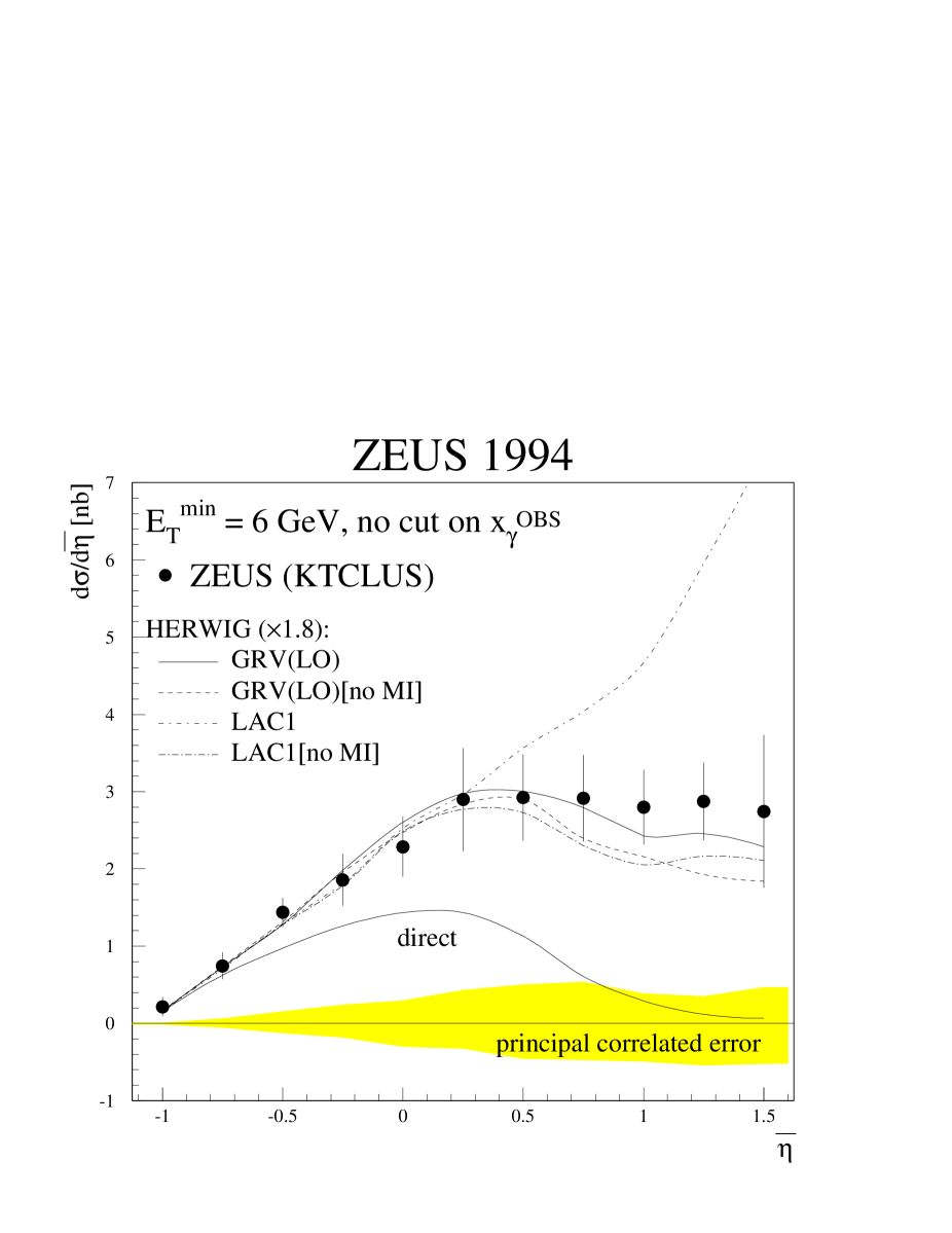
Figure 3: $d\sigma/d\bar{\eta}$ for $ep\rightarrow e+$ dijets $+X$ in the range $|\Delta\eta|<0.5$, $0.2<y<0.8$ and for virtualities of the exchanged photon $<4$ GeV² and for $E_{T}^{jet}$ integrated above $E_{T}^{min}=6$ GeV. The cross section is measured using the KTCLUS algorithm and is compared to the expectations of various HERWIG MC simulations (see text). The errors bars represent the combined systematic and statistical uncertainty, excluding the principal correlated uncertainties which are shown in the shaded band, see text.

7.2 Cross Sections with ${\boldmath x_{\gamma}^{OBS}}$ Cuts

Two regions have been selected:

1. $x_{\gamma}^{OBS}\geq 0.75$: direct photoproduction.

2. $0.3<x_{\gamma}^{OBS}<0.75$: resolved photoproduction excluding the low-$x_{\gamma}^{OBS}$ region.

For each $x_{\gamma}^{OBS}$ region, the cross sections $d\sigma/d\bar{\eta}$ for $ep\rightarrow e+$ dijets $+X$ in the range $|\Delta\eta|<0.5$, $0.2<y<0.8$ and for virtualities of the exchanged photon $<4$ GeV² are measured for four different values of the $E_{T}^{jet}$ threshold, $E_{T}^{min}$ = 6, 8, 11 and 15 GeV. The cross sections are measured for the three different jet algorithms discussed in section 3. The results are given in Tables 2 to 7 and are displayed in Fig. 4 together with the results of the NLO QCD calculation from Klasen and Kramer [29] using the NLO GRV [23] parton distributions for the photon and the CTEQ3M [30] parton distributions for the proton and employing two different values of the $R_{\rm sep}$ parameter: $R_{\rm sep}=1$ (solid curve) and $R_{\rm sep}~{}=~{}2$ (dashed curve). Since the jets may be accompanied by other soft gluons (outside the jets), there is a potential problem when the two jets have the same $E_{T}^{jet}$. The infrared singularity associated with summing the soft gluon contributions is usually cancelled by the singularity coming from the one-loop contribution. For two jets with the same $E_{T}^{jet}$, some of the phase space for the soft gluon terms is restricted and an incomplete cancellation may occur in some calculations. As a consequence, Klasen and Kramer [29] have allowed the second jet to have an $E_{T}^{jet}$ less than $E_{T}^{min}$ if the third (unobserved gluon) jet has a transverse energy of less than 1 GeV. However, the cross section is then sensitive to changes in the value used for this cut on the third jet. Harris and Owens [31] have applied a low cutoff on the energy of the very soft gluons and found that the dependence of the cross sections on the value of the low energy cutoff used is much less than the quoted errors on the data. These different approaches account for the differences between the theory curves shown later.

The photoproduction cross section for $x_{\gamma}^{OBS}\geq 0.75$ and $E_{T}^{min}=6$ GeV (Fig. 4a) rises from around 0.2 nb at $\bar{\eta}=-1$ to a maximum value of around 1.8 nb at $\bar{\eta}=0$, decreasing back to 0.2 nb by $\bar{\eta}=1$. This decrease arises from the cutoff on the minimum $E_{T}^{jet}$ and the cuts on $y$. The EUCELL jet cross sections are systematically higher than the PUCELL cross sections, which in turn are slightly above the KTCLUS cross sections. This behaviour is qualitatively similar for the higher $E_{T}^{min}$ cross sections (Figs. 4b-d), where the maximum value of the cross section falls and occurs at steadily higher $\bar{\eta}$ as the minimum $E_{T}^{jet}$ cut increases. The PUCELL and KTCLUS cross sections are in good agreement with the NLO curve calculated with $R_{\rm sep}=1$ for all $\bar{\eta}$ and for all four $E_{T}^{jet}$ thresholds, except for the most negative values of $\bar{\eta}$ in the lower $E_{T}^{min}$ cross sections, where the trend is for the calculation to lie above the data. The $R_{\rm sep}=2$ curve lies above all the data at most values of $\bar{\eta}$. In the data the separation between EUCELL, PUCELL and KTCLUS becomes less significant at higher $E_{T}^{jet}$. However, the separation between the two theory curves remains significant.

Figure 4: $d\sigma/d\bar{\eta}$ for $ep\rightarrow e+$ dijets $+X$ in the range $|\Delta\eta|<0.5$, $0.2<y<0.8$ and for virtualities of the exchanged photon $<4$ GeV² and for $E_{T}^{min}$ = 6, 8, 11 and 15 GeV. Figures (a-d) are the cross sections measured in the range $x_{\gamma}^{OBS}\geq 0.75$; figures (e-h) are for the range $0.3<x_{\gamma}^{OBS}<0.75$. The cross sections are measured using three different jet algorithms and are compared to NLO QCD calculations using $R_{sep}$ = 1 (solid curves) and $R_{sep}$ = 2 (dashed curves), see text for details. The errors bars represent the combined systematic and statistical uncertainty, excluding the principal correlated uncertainties, which are shown in the shaded band (see text). The band indicates the maximum uncertainty for the three jet finders. The individual uncertainty for each jet finder is given in the table.

The photoproduction cross section for $0.3<x_{\gamma}^{OBS}<0.75$ and $E_{T}^{min}=6$ GeV (Fig. 4e) rises from around 0.8 nb at $\bar{\eta}=-0.25$ to a maximum value of 1.5 nb for PUCELL and KTCLUS, and of 3 nb for EUCELL, at $\bar{\eta}=0$, followed by a decrease back to 0.2 nb by $\bar{\eta}=1.5$. The EUCELL jet cross sections are again systematically higher than the PUCELL cross sections which are again slightly above those for KTCLUS. This behaviour is once more qualitatively similar for the higher $E_{T}^{jet}$ cross sections (Figs. 4f-h), where the maximum value of the cross section falls and occurs at steadily higher $\bar{\eta}$. In the data the separation between EUCELL and the two other jet algorithms is larger than in the direct case - a factor of two at the lowest $E_{T}^{jet}$ values - but again becomes less significant at higher $E_{T}^{jet}$. In the theory, the differences between the curves with different $R_{\rm sep}$ again show the same trend as the data, with the $R_{\rm sep}=2$ curves being higher than those for $R_{\rm sep}=1$. However, for the cross sections with $E_{T}^{min}=6$ GeV and 8 GeV, the NLO QCD curves lie significantly below the data. For higher $E_{T}^{min}$ values the calculations are broadly consistent with the data.

In Fig. 5 the KTCLUS jet cross sections are shown again, with Klasen and Kramer’s NLO QCD calculations (with $R_{\rm sep}=1$) employing two different parton distribution functions for the photon - namely those of NLO GRV(solid curves [23]) and GS (dashed curves [32]). It can be seen that the agreement is in general good for both distribution functions, except in the two lowest $E_{T}^{jet}$ regions of the resolved cross section (Fig 5e,f) where the QCD calculations are significantly below the data. Perhaps surprisingly, the difference between the photon parton distributions is largest in the direct photoproduction region. This is due to differences between the quark distributions in the photon for $x_{\gamma}>0.8$, where they are poorly constrained by photon structure function measurements at $e^{+}e^{-}$ colliders. These differences persist at high $E_{T}^{jet}$. Also shown in Fig. 5 is a NLO QCD calculation (again with $R_{\rm sep}=1$) from Harris and Owens using NLO GRV $\overline{\rm MS}$ for the photon, and NLO CTEQ4 $\overline{\rm MS}$ for the proton. At high $x_{\gamma}^{OBS}$ there is again good agreement with the measurements, but at low $x_{\gamma}^{OBS}$ the disagreement in the two lowest $E_{T}^{jet}$ regions is large. At higher $E_{T}^{jet}$ values, the data and calculations are consistent.

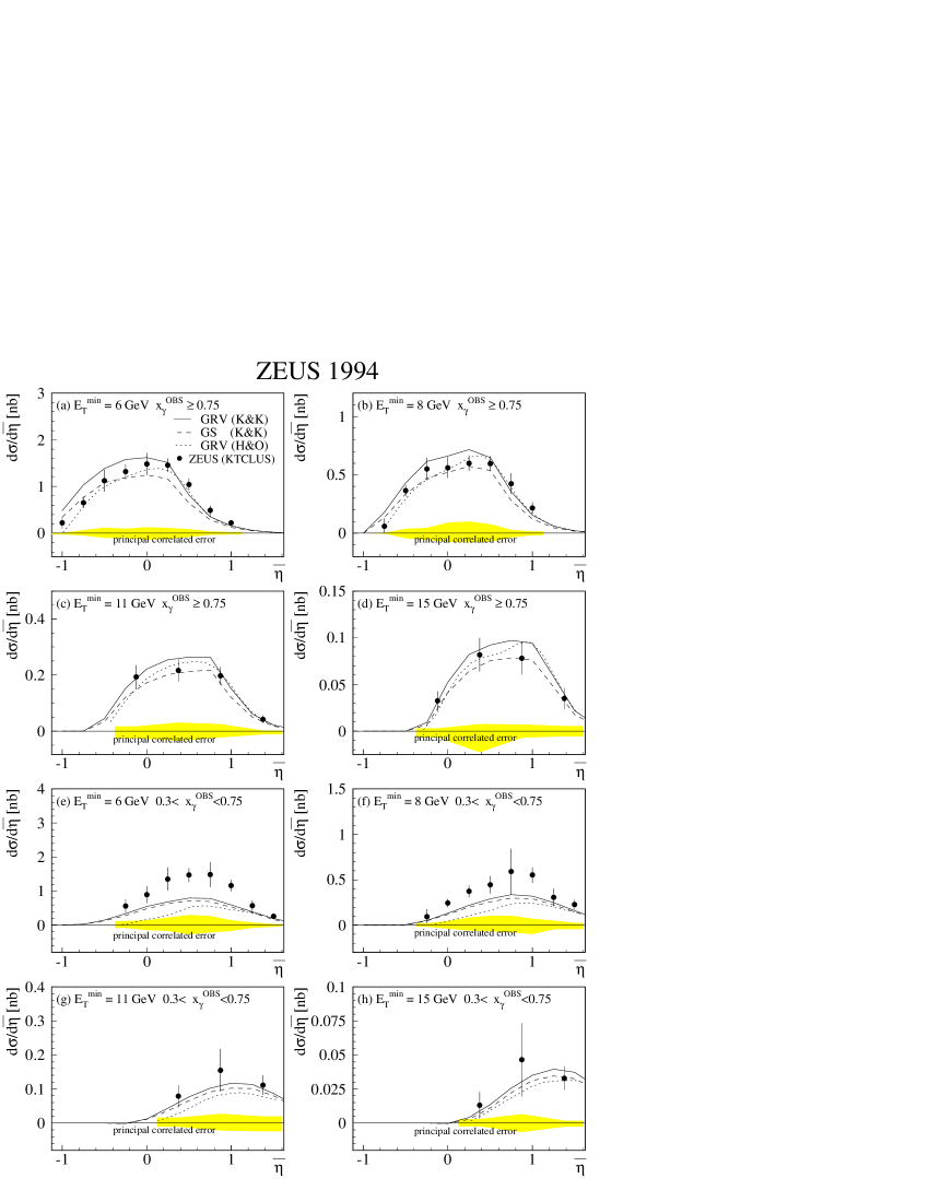
Figure 5: $d\sigma/d\bar{\eta}$ for $ep\rightarrow e+$ dijets $+X$ in the range $|\Delta\eta|<0.5$, $0.2<y<0.8$ and for virtualities of the exchanged photon $<4$ GeV² and for $E_{T}^{min}$ = 6, 8, 11 and 15 GeV. Figures (a-d) are the cross sections measured in the range $x_{\gamma}^{OBS}\geq 0.75$; figures (e-h) are for the range $0.3<x_{\gamma}^{OBS}<0.75$. The cross sections are measured using the KTCLUS jet algorithm and are compared to NLO QCD calculations from Klasen and Kramer, for two different parton distributions in the photon , GRV and GS, and from Harris and Owens using GRV (see text for details). All three calculations use $R_{sep}$ = 1. The errors bars represent the combined systematic and statistical uncertainty, excluding the principal correlated uncertainties which are shown in the shaded band (see text).

8 Conclusions

Photoproduced dijet cross sections $d\sigma/d\bar{\eta}$ have been measured in the hadronic final state for different kinematic regions and are found to be consistent with the general expectations of QCD, in the sense that both resolved and direct processes are observed in the data.

Quantitatively, it is found that Monte Carlo simulations both with and without multiparton interactions are capable of describing the $\bar{\eta}$ dependence of the cross section when no $x_{\gamma}^{OBS}$ cuts are applied, although simulations which use multiparton interactions to simulate an underlying event are slightly favoured and also give a better description of the jet profiles.

The measured cross sections vary by up to a factor of two when different cone or clustering algorithms are used for the definition of jets. This behaviour is similar to that predicted from the theoretical calculations by choosing the $R_{\rm sep}$ parameter in order to reproduce the different jet algorithms.

Comparison of the direct photon cross sections ($x_{\gamma}^{OBS}>0.75$) with NLO QCD calculations shows good agreement in both shape and magnitude over a wide range of $E_{T}^{jet}$ and $\eta^{jet}$ and for the three different jet definitions. It also displays a sensitivity to the photon structure at large $x_{\gamma}$.

Calculations for the resolved photon cross sections in the region $0.3<x_{\gamma}^{OBS}<0.75$ which include jets with 6 GeV$<E_{T}^{jet}<11$ GeV are found to lie below the data. However, for higher jet energies the calculations are consistent with the data.

$\bar{\eta}$	$\displaystyle\frac{d\sigma}{d\bar{\eta}}$ [nb]	stat. [nb]	syst. [nb]	corrl. syst. [nb]
$E_{T}^{min}>6~{}{\rm GeV}$
$-1.000$	0.22	0.02	0.12	$+0.01$	$-0.01$
$-0.750$	0.75	0.05	0.16	$+0.06$	$-0.05$
$-0.500$	1.44	0.08	0.17	$+0.15$	$-0.13$
$-0.250$	1.86	0.08	0.32	$+0.24$	$-0.18$
$0.000$	2.29	0.09	0.38	$+0.30$	$-0.30$
$0.250$	2.90	0.10	0.66	$+0.43$	$-0.33$
$0.500$	2.92	0.10	0.55	$+0.50$	$-0.46$
$0.750$	2.91	0.11	0.55	$+0.54$	$-0.47$
$1.000$	2.80	0.11	0.47	$+0.38$	$-0.49$
$1.250$	2.87	0.12	0.49	$+0.35$	$-0.54$
$1.500$	2.74	0.11	0.98	$+0.46$	$-0.52$
$E_{T}^{min}>8~{}{\rm GeV}$
$-0.750$	0.06	0.01	0.06	$+0.01$	$-0.01$
$-0.500$	0.38	0.04	0.02	$+0.04$	$-0.03$
$-0.250$	0.65	0.05	0.08	$+0.07$	$-0.08$
$0.000$	0.81	0.05	0.09	$+0.13$	$-0.11$
$0.250$	0.97	0.06	0.11	$+0.19$	$-0.13$
$0.500$	1.07	0.06	0.17	$+0.18$	$-0.15$
$0.750$	1.16	0.06	0.20	$+0.17$	$-0.14$
$1.000$	0.99	0.06	0.12	$+0.15$	$-0.17$
$1.250$	0.82	0.06	0.12	$+0.12$	$-0.18$
$1.500$	0.71	0.05	0.08	$+0.13$	$-0.15$
$E_{T}^{min}>11~{}{\rm GeV}$
$-0.125$	0.21	0.02	0.02	$+0.02$	$-0.02$
$0.375$	0.29	0.02	0.02	$+0.05$	$-0.04$
$0.875$	0.37	0.02	0.06	$+0.06$	$-0.05$
$1.375$	0.23	0.02	0.02	$+0.03$	$-0.05$
$E_{T}^{min}>15~{}{\rm GeV}$
$-0.125$	0.033	0.008	0.005	$+0.003$	$-0.004$
$0.375$	0.093	0.012	0.036	$+0.011$	$-0.023$
$0.875$	0.126	0.014	0.027	$+0.014$	$-0.014$
$1.375$	0.079	0.010	0.016	$+0.012$	$-0.010$

Table 1: The cross sections for KTCLUS for the whole $x_{\gamma}^{OBS}$ range. The third and fourth columns represent the statistical and systematic uncertainties, excluding the principal correlated uncertainties which are shown in the fifth column, see text.

$\bar{\eta}$	$\displaystyle\frac{d\sigma}{d\bar{\eta}}$ [nb]	stat. [nb]	syst. [nb]	corrl. syst. [nb]
$E_{T}^{min}>6~{}{\rm GeV}$
$-1.000$	0.22	0.03	0.05	$+0.02$	$-0.02$
$-0.750$	0.81	0.06	0.09	$+0.04$	$-0.08$
$-0.500$	1.29	0.08	0.15	$+0.14$	$-0.09$
$-0.250$	1.47	0.08	0.14	$+0.13$	$-0.15$
$0.000$	1.65	0.08	0.21	$+0.14$	$-0.14$
$0.250$	1.61	0.08	0.20	$+0.16$	$-0.15$
$0.500$	1.03	0.06	0.20	$+0.07$	$-0.09$
$0.750$	0.59	0.04	0.13	$+0.05$	$-0.04$
$1.000$	0.21	0.02	0.03	$+0.02$	$-0.02$
$E_{T}^{min}>8~{}{\rm GeV}$
$-0.750$	0.08	0.01	0.03	$+0.01$	$-0.01$
$-0.500$	0.38	0.04	0.05	$+0.02$	$-0.04$
$-0.250$	0.60	0.05	0.05	$+0.04$	$-0.05$
$0.000$	0.66	0.05	0.14	$+0.10$	$-0.07$
$0.250$	0.64	0.05	0.08	$+0.11$	$-0.09$
$0.500$	0.61	0.05	0.08	$+0.08$	$-0.08$
$0.750$	0.51	0.04	0.09	$+0.03$	$-0.04$
$1.000$	0.21	0.02	0.03	$+0.01$	$-0.02$
$E_{T}^{min}>11~{}{\rm GeV}$
$-0.125$	0.23	0.02	0.04	$+0.01$	$-0.02$
$0.375$	0.22	0.02	0.02	$+0.03$	$-0.03$
$0.875$	0.22	0.02	0.03	$+0.02$	$-0.03$
$1.375$	0.05	0.01	0.02	$+0.01$	$-0.01$
$E_{T}^{min}>15~{}{\rm GeV}$
$-0.125$	0.032	0.008	0.009	$+0.008$	$-0.003$
$0.375$	0.078	0.011	0.011	$+0.012$	$-0.024$
$0.875$	0.083	0.012	0.006	$+0.013$	$-0.009$
$1.375$	0.039	0.008	0.014	$+0.004$	$-0.007$

Table 2: The cross sections for PUCELL and $x_{\gamma}^{OBS}\geq 0.75$. The third and fourth columns represent the statistical and systematic uncertainties, excluding the principal correlated uncertainties which are shown in the fifth column, see text.

$\bar{\eta}$	$\displaystyle\frac{d\sigma}{d\bar{\eta}}$ [nb]	stat. [nb]	syst. [nb]	corrl. syst. [nb]
$E_{T}^{min}>6~{}{\rm GeV}$
$-0.250$	0.73	0.06	0.17	$+0.15$	$-0.09$
$0.000$	1.13	0.07	0.19	$+0.19$	$-0.17$
$0.250$	1.61	0.08	0.26	$+0.26$	$-0.25$
$0.500$	1.81	0.09	0.43	$+0.29$	$-0.29$
$0.750$	1.90	0.10	0.32	$+0.31$	$-0.34$
$1.000$	1.37	0.09	0.20	$+0.23$	$-0.19$
$1.250$	0.73	0.06	0.21	$+0.10$	$-0.10$
$1.500$	0.32	0.03	0.06	$+0.06$	$-0.06$
$E_{T}^{min}>8~{}{\rm GeV}$
$-0.250$	0.12	0.02	0.04	$+0.02$	$-0.02$
$0.000$	0.26	0.03	0.04	$+0.05$	$-0.03$
$0.250$	0.48	0.04	0.06	$+0.08$	$-0.10$
$0.500$	0.54	0.04	0.10	$+0.11$	$-0.09$
$0.750$	0.62	0.05	0.18	$+0.11$	$-0.10$
$1.000$	0.62	0.05	0.19	$+0.12$	$-0.12$
$1.250$	0.35	0.04	0.05	$+0.06$	$-0.05$
$1.500$	0.22	0.03	0.04	$+0.04$	$-0.04$
$E_{T}^{min}>11~{}{\rm GeV}$
$0.375$	0.09	0.01	0.02	$+0.01$	$-0.02$
$0.875$	0.16	0.02	0.06	$+0.03$	$-0.03$
$1.375$	0.12	0.01	0.02	$+0.02$	$-0.02$
$E_{T}^{min}>15~{}{\rm GeV}$
$0.375$	0.011	0.003	0.004	$+0.004$	$-0.002$
$0.875$	0.050	0.009	0.018	$+0.002$	$-0.007$
$1.375$	0.034	0.006	0.005	$+0.003$	$-0.005$

Table 3: The cross sections for PUCELL and $0.30<x_{\gamma}^{OBS}<0.75$. The third and fourth columns represent the statistical and systematic uncertainties, excluding the principal correlated uncertainties which are shown in the fifth column, see text.

$\bar{\eta}$	$\displaystyle\frac{d\sigma}{d\bar{\eta}}$ [nb]	stat. [nb]	syst. [nb]	corrl. syst. [nb]
$E_{T}^{min}>6~{}{\rm GeV}$
$-1.000$	0.27	0.03	0.04	$+0.02$	$-0.01$
$-0.750$	0.92	0.06	0.21	$+0.09$	$-0.10$
$-0.500$	1.52	0.08	0.20	$+0.18$	$-0.12$
$-0.250$	1.78	0.09	0.11	$+0.17$	$-0.17$
$0.000$	1.96	0.09	0.20	$+0.20$	$-0.19$
$0.250$	1.91	0.09	0.22	$+0.18$	$-0.19$
$0.500$	1.27	0.07	0.27	$+0.09$	$-0.13$
$0.750$	0.62	0.04	0.16	$+0.06$	$-0.05$
$1.000$	0.27	0.03	0.05	$+0.02$	$-0.02$
$E_{T}^{min}>8~{}{\rm GeV}$
$-0.750$	0.08	0.01	0.05	$+0.01$	$-0.01$
$-0.500$	0.44	0.04	0.05	$+0.07$	$-0.04$
$-0.250$	0.69	0.05	0.05	$+0.07$	$-0.03$
$0.000$	0.75	0.05	0.14	$+0.13$	$-0.10$
$0.250$	0.77	0.05	0.03	$+0.13$	$-0.10$
$0.500$	0.72	0.05	0.08	$+0.13$	$-0.09$
$0.750$	0.55	0.04	0.12	$+0.05$	$-0.05$
$1.000$	0.27	0.03	0.05	$+0.02$	$-0.02$
$E_{T}^{min}>11~{}{\rm GeV}$
$-0.125$	0.23	0.02	0.04	$+0.02$	$-0.02$
$0.375$	0.27	0.02	0.02	$+0.03$	$-0.05$
$0.875$	0.25	0.02	0.03	$+0.03$	$-0.03$
$1.375$	0.06	0.01	0.01	$+0.01$	$-0.01$
$E_{T}^{min}>15~{}{\rm GeV}$
$-0.125$	0.036	0.009	0.007	$+0.007$	$-0.004$
$0.375$	0.082	0.012	0.010	$+0.017$	$-0.017$
$0.875$	0.095	0.013	0.006	$+0.017$	$-0.011$
$1.375$	0.045	0.007	0.013	$+0.004$	$-0.006$

Table 4: The cross sections for EUCELL and $x_{\gamma}^{OBS}\geq 0.75$. The third and fourth columns represent the statistical and systematic uncertainties, excluding the principal correlated uncertainties which are shown in the fifth column, see text.

$\bar{\eta}$	$\displaystyle\frac{d\sigma}{d\bar{\eta}}$ [nb]	stat. [nb]	syst. [nb]	corrl. syst. [nb]
$E_{T}^{min}>6~{}{\rm GeV}$
$-0.250$	1.11	0.07	0.43	$+0.21$	$-0.18$
$0.000$	1.95	0.10	0.16	$+0.33$	$-0.36$
$0.250$	2.81	0.12	0.26	$+0.47$	$-0.47$
$0.500$	2.82	0.12	0.51	$+0.45$	$-0.45$
$0.750$	2.98	0.13	0.57	$+0.49$	$-0.49$
$1.000$	2.22	0.12	0.38	$+0.31$	$-0.32$
$1.250$	1.14	0.08	0.30	$+0.15$	$-0.16$
$1.500$	0.45	0.04	0.19	$+0.10$	$-0.10$
$E_{T}^{min}>8~{}{\rm GeV}$
$-0.250$	0.15	0.02	0.06	$+0.05$	$-0.03$
$0.000$	0.44	0.04	0.09	$+0.09$	$-0.08$
$0.250$	0.68	0.05	0.25	$+0.12$	$-0.13$
$0.500$	0.73	0.05	0.17	$+0.17$	$-0.13$
$0.750$	0.93	0.06	0.45	$+0.21$	$-0.17$
$1.000$	0.88	0.07	0.09	$+0.19$	$-0.17$
$1.250$	0.57	0.05	0.09	$+0.07$	$-0.09$
$1.500$	0.30	0.03	0.10	$+0.06$	$-0.07$
$E_{T}^{min}>11~{}{\rm GeV}$
$0.375$	0.11	0.01	0.03	$+0.02$	$-0.01$
$0.875$	0.24	0.02	0.06	$+0.04$	$-0.05$
$1.375$	0.17	0.02	0.02	$+0.04$	$-0.04$
$E_{T}^{min}>15~{}{\rm GeV}$
$0.375$	0.019	0.005	0.015	$+0.004$	$-0.005$
$0.875$	0.057	0.009	0.024	$+0.007$	$-0.006$
$1.375$	0.047	0.008	0.006	$+0.007$	$-0.005$

Table 5: The cross sections for EUCELL and $0.30<x_{\gamma}^{OBS}<0.75$. The third and fourth columns represent the statistical and systematic uncertainties, excluding the principal correlated uncertainties which are shown in the fifth column, see text.

$\bar{\eta}$	$\displaystyle\frac{d\sigma}{d\bar{\eta}}$ [nb]	stat. [nb]	syst. [nb]	corrl. syst. [nb]
$E_{T}^{min}>6~{}{\rm GeV}$
$-1.000$	0.22	0.03	0.12	$+0.01$	$-0.02$
$-0.750$	0.66	0.05	0.10	$+0.06$	$-0.05$
$-0.500$	1.12	0.07	0.22	$+0.12$	$-0.10$
$-0.250$	1.32	0.07	0.15	$+0.10$	$-0.09$
$0.000$	1.48	0.07	0.22	$+0.13$	$-0.14$
$0.250$	1.46	0.07	0.13	$+0.11$	$-0.12$
$0.500$	1.05	0.06	0.11	$+0.08$	$-0.08$
$0.750$	0.49	0.04	0.09	$+0.04$	$-0.03$
$1.000$	0.22	0.03	0.05	$+0.02$	$-0.02$
$E_{T}^{min}>8~{}{\rm GeV}$
$-0.750$	0.06	0.01	0.06	$+0.01$	$-0.01$
$-0.500$	0.36	0.04	0.03	$+0.04$	$-0.04$
$-0.250$	0.55	0.05	0.09	$+0.04$	$-0.06$
$0.000$	0.56	0.04	0.08	$+0.09$	$-0.07$
$0.250$	0.60	0.04	0.05	$+0.10$	$-0.08$
$0.500$	0.60	0.04	0.05	$+0.08$	$-0.07$
$0.750$	0.42	0.04	0.08	$+0.03$	$-0.03$
$1.000$	0.22	0.03	0.04	$+0.01$	$-0.02$
$E_{T}^{min}>11~{}{\rm GeV}$
$-0.125$	0.19	0.02	0.04	$+0.02$	$-0.02$
$0.375$	0.22	0.02	0.03	$+0.03$	$-0.03$
$0.875$	0.20	0.02	0.03	$+0.02$	$-0.02$
$1.375$	0.04	0.01	0.01	$+0.01$	$-0.01$
$E_{T}^{min}>15~{}{\rm GeV}$
$-0.125$	0.033	0.008	0.006	$+0.003$	$-0.007$
$0.375$	0.082	0.012	0.014	$+0.008$	$-0.022$
$0.875$	0.078	0.011	0.014	$+0.007$	$-0.007$
$1.375$	0.035	0.007	0.009	$+0.005$	$-0.005$

Table 6: The cross sections for KTCLUS and $x_{\gamma}^{OBS}\geq 0.75$. The third and fourth columns represent the statistical and systematic uncertainties, excluding the principal correlated uncertainties which are shown in the fifth column, see text.

$\bar{\eta}$	$\displaystyle\frac{d\sigma}{d\bar{\eta}}$ [nb]	stat. [nb]	syst. [nb]	corrl. syst. [nb]
$E_{T}^{min}>6~{}{\rm GeV}$
$-0.250$	0.56	0.05	0.20	$+0.11$	$-0.08$
$0.000$	0.89	0.06	0.24	$+0.14$	$-0.14$
$0.250$	1.35	0.07	0.33	$+0.22$	$-0.16$
$0.500$	1.47	0.07	0.19	$+0.30$	$-0.26$
$0.750$	1.49	0.08	0.36	$+0.26$	$-0.21$
$1.000$	1.16	0.07	0.15	$+0.14$	$-0.16$
$1.250$	0.57	0.05	0.14	$+0.07$	$-0.07$
$1.500$	0.26	0.03	0.07	$+0.02$	$-0.04$
$E_{T}^{min}>8~{}{\rm GeV}$
$-0.250$	0.09	0.02	0.08	$+0.02$	$-0.02$
$0.000$	0.25	0.03	0.04	$+0.04$	$-0.04$
$0.250$	0.37	0.03	0.06	$+0.08$	$-0.06$
$0.500$	0.45	0.04	0.09	$+0.10$	$-0.07$
$0.750$	0.59	0.05	0.25	$+0.10$	$-0.08$
$1.000$	0.55	0.05	0.07	$+0.07$	$-0.09$
$1.250$	0.31	0.03	0.09	$+0.05$	$-0.04$
$1.500$	0.23	0.03	0.05	$+0.02$	$-0.04$
$E_{T}^{min}>11~{}{\rm GeV}$
$0.375$	0.08	0.01	0.03	$+0.02$	$-0.01$
$0.875$	0.16	0.02	0.06	$+0.03$	$-0.02$
$1.375$	0.11	0.01	0.03	$+0.02$	$-0.02$
$E_{T}^{min}>15~{}{\rm GeV}$
$0.375$	0.013	0.004	0.009	$+0.003$	$-0.002$
$0.875$	0.046	0.008	0.026	$+0.007$	$-0.007$
$1.375$	0.033	0.006	0.006	$+0.002$	$-0.003$

Table 7: The cross sections for KTCLUS and $0.30<x_{\gamma}^{OBS}<0.75$. The third and fourth columns represent the statistical and systematic uncertainties, excluding the principal correlated uncertainties which are shown in the fifth column, see text.

References

- [1] ZEUS Collab., M. Derrick et al., Phys. Lett. B348 (1995) 665.
- [2] H1 Collab., C. Adloff et al., DESY 97-164, to appear in Z. Phys C.
- [3] J. R. Forshaw and R. G. Roberts, Phys. Lett. B319 (1993) 539.
- [4] ZEUS Collab., The ZEUS detector, Status Report (1993).
- [5] C. Alvisi et al., Nucl. Instr. and Meth. A305 (1991) 30.
-
[6]
N. Harnew et al., Nucl. Inst. Meth. A279 (1989) 290;
B. Foster et al., Nucl. Phys. B, (Proc. Suppl.) 32 (1993) 181;
B. Foster et al., Nucl. Inst. Meth. A338 (1994) 254. -
[7]
M. Derrick et al., Nucl. Instr. and Meth. A309 (1991)
77;
A. Andresen et al., Nucl. Instr. and Meth. A309 (1991) 101;
A. Bernstein et al., Nucl. Instr. and Meth. A336 (1993) 23. - [8] J. Andruszków et al., DESY 92-066.
- [9] J. E. Huth et al., Proc. of the 1990 DPF Summer Study on High Energy Physics, Snowmass, Colorado, edited by E.L. Berger, (World Scientific, Singapore, 1992) 134.
-
[10]
W. T. Giele and W. B. Kilgore, Phys. Rev. D55 (1997) 7183;
W. B. Kilgore, hep-ph/9705384 ;
M. H. Seymour, hep-ph/9797338. - [11] CDF Collab., F. Abe et al., Phys. Rev. D45 (1992) 1448.
- [12] S. Catani, Yu.L. Dokshitzer, M.H. Seymour and B.R. Webber, Nucl. Phys. B406 (1993) 187.
- [13] S.D. Ellis and D.E. Soper, Phys. Rev. D48 (1993) 3160.
- [14] S.D. Ellis, Z. Kunszt and D.E. Soper, Phys. Rev. Lett. 69 (1992) 3615.
- [15] J. M. Butterworth, L. Feld, M. Klasen and G. Kramer, hep-ph/9608481; Proceedings of the Workshop on “Future Physics at HERA”, Editors: G. Ingelman, A. DeRoeck, R. Klanner, DESY 1996, p. 554.
- [16] ZEUS Collab., M. Derrick et al., Phys. Lett. B316 (1993) 412.
- [17] ZEUS Collab., M. Derrick et al., Phys. Lett. B322 (1994) 287.
- [18] F. Jacquet and A. Blondel, in Proceedings of the study of an facility for Europe, Hamburg, ed. U. Amaldi, (DESY 79/48, 1979) 391.
- [19] ZEUS Collab., M. Derrick et al., Z. Phys. C72 (1996) 399.
-
[20]
L. Feld, Ph.D. thesis BONN-IR-96-17, Bonn University, December 1996;
R. Saunders, Ph.D. thesis, University College London 1997. - [21] G. Marchesini et al., Comp. Phys. Comm. 67 (1992) 465.
- [22] T. Sjöstrand, Comp. Phys. Comm. 82 (1994) 74.
- [23] M. Glück, E. Reya and A. Vogt, Phys. Rev. D46 (1992) 1973.
- [24] A. D. Martin, W.J. Stirling and R.G. Roberts, Phys. Rev. D50 (1994) 6734.
-
[25]
T. Sjöstrand and M. van Zijl, Phys. Rev. D36 (1987) 2019;
G. A. Schuler and T. Sjöstrand, Phys. Lett. B300 (1993) 169; Nucl. Phys. B407 (1993) 539;
J. M. Butterworth and J. R. Forshaw, J. Phys. G19 (1993) 1657. - [26] J. M. Butterworth, J. R. Forshaw and M. H. Seymour, Z. Phys. C72 (1996) 637.
- [27] H1 Collab., S. Aid et al., Z. Phys. C70 (1996) 17.
- [28] H. Abramowicz, K. Charchula and A. Levy, Phys. Lett. B269 (1991) 458.
- [29] M. Klasen and G. Kramer, DESY-96-246, hep-ph/9611450.
-
[30]
CTEQ Collab., J. Botts et al., Phys. Lett. B304 (1993) 159;
CTEQ Collab., H.L. Lai et al., Phys. Rev. D51 (1995) 4763. - [31] B. W. Harris and J. F. Owens, FSU-HEP-970411, hep-ph/9704324, to be published in Phys. Rev. D.
- [32] L.E. Gordon and J.K. Storrow, Phys. Lett. B291 (1992) 320.