Spin Analysis of the Process $\rm e^{+}e^{-}\rightarrow\tau^{+}\tau^{-}$ at LEP

Abstract

Using the data collected by the four experiments at LEP during 1990–1994, a precise measurement of the $\tau$ longitudinal polarisation (${\cal P}_{\tau}$) has been performed, as well as the measurement of the transverse–transverse (${\rm C_{TT}}$) and transverse–normal (${\rm C_{TN}}$) $\tau$ spin correlations. From the ${\cal P}_{\tau}$ measurement, assuming lepton universality of the neutral currents, the effective weak mixing angle has been determined to be $\sin^{2}\theta_{W}=0.2325\pm 0.0006$. The Standard Model predictions are consistent with the measured results.

1 INTRODUCTION

It is a well established principle that weak interactions violate parity. This fact constitutes a powerful tool for performing high precision tests of the Standard Model [1].

At LEP, where $\rm e^{+}e^{-}\rightarrow\rm f\,\overline{f}\$ ($f=e,\ \mu,\ \tau$) interactions are produced at centre of mass energies close to $\rm M_{Z}$, the study of observables related to the spin of the final state fermions provides an accurate determination of the vector and axial–vector coupling of the fermions to the Z boson. Only in the $\rm e^{+}e^{-}\rightarrow\tau^{+}\tau^{-}$ processes, where both taus decay before entering the detector, we can extract information on the final state spin configuration by analysing the $\tau$ decay process itself.

The cross section describing the $\rm e^{+}e^{-}\rightarrow\tau^{+}\tau^{-}$ process can be written in terms of the final state taus spin components as follows [2]:

$$\frac{d^{5}\sigma}{ds_{\tau^{\pm}}d\Omega} = \frac{1}{4}|P(q^{2})|^{2}\{{C_{0}}\,(1+\cos^{2}\theta)$$

$$+ C_{1}\,2\cos\theta$$

$$- D_{0}\,(s_{\tau^{-}}^{L}-s_{\tau^{+}}^{L})\,(1+\cos^{2}\theta)$$

$$- D_{1}\,(s_{\tau^{-}}^{L}-s_{\tau^{+}}^{L})\,2\cos\theta$$

$$- C_{0}\,s_{\tau^{-}}^{L}s_{\tau^{+}}^{L}\,(1+\cos^{2}\theta)$$

$$- C_{1}\,s_{\tau^{-}}^{L}s_{\tau^{+}}^{L}\,2\cos\theta$$

$$+ C_{2}\,(s_{\tau^{-}}^{N}s_{\tau^{+}}^{N}-s_{\tau^{-}}^{T}s_{\tau^{+}}^{T})\,\sin^{2}\theta$$

$$+ D_{2}\,(s_{\tau^{-}}^{N}s_{\tau^{+}}^{T}+s_{\tau^{-}}^{T}s_{\tau^{+}}^{N})\,\sin^{2}\theta\}$$

where $P(q^{2})$ contains the Z propagator and $\theta$ is the $\tau^{-}$ polar angle with respect to the incident $e^{-}$ flight direction. $s_{\tau^{-}}^{L}$ is the (Longitudinal) projection of the spin of the $\tau$ along its flight direction in the lab frame, $s_{\tau^{-}}^{T}$ the (Transverse) projection in the plane defined by the incoming $e^{-}$ and the outgoing $\tau^{-}$ and $s_{\tau^{-}}^{N}$ the component Normal to these two.

The functions $C_{i}$ and $D_{i}$ ($i=0,\ 1,\ 2$) depend on the couplings of the Z to the leptons ($v_{e},\ a_{e},\ v_{\tau},\ a_{\tau}$). In the following sections we will exploit the symmetries of the cross section in order to define quantities (in terms of $C$ and $D$) related to the $\tau$ spin which can be measured accurately at LEP: these are the $\tau$ longitudinal polarisation (${\cal P}_{\tau}$) and the transverse–transverse (${\rm C_{TT}}$) and transverse–normal (${\rm C_{TN}}$) $\tau$ spin correlations.

2 $\tau$ LONGITUDINAL POLARISATION

Due to the parity violation of the neutral currents, there is a difference in the production cross section (for a given $\cos\theta$ value) of the $\tau^{-}$ with left (L) and right (R) helicity. The $\tau$ polarisation asymmetry is defined as:

$${\cal P}_{\tau}\ \equiv\ {\sigma_{R}-\sigma_{L}\over\sigma_{R}+\sigma_{L}}\ =\ -\ {D_{0}\over C_{0}}$$ (2)

where $\sigma_{L(R)}\ \equiv\ \sigma\,(e^{-}e^{+}\rightarrow\tau^{-}_{L(R)}\tau^{+}_{R(L)})$. Using equation (1), ${\cal P}_{\tau}$ can be expressed in terms of $\cos\theta$ as:

$${\cal P}_{\tau}\,(\cos\theta)\ =\ -\ {{\cal A}_{\tau}\,(1+\cos^{2}\theta)\,+\,{\cal A}_{e}\,2\cos\theta\over(1+\cos^{2}\theta)\,+\,{\cal A}_{\tau}{\cal A}_{e}\,2\cos\theta}$$ (3)

being

$${\cal A}_{\ell}\ \equiv\ {\textstyle{2\,a_{\ell}\,v_{\ell}}\over\textstyle{|a_{\ell}|^{2}+|v_{\ell}|^{2}}}\ =\ {2\,(1-4\sin^{2}\theta_{W})\over 1+(1-4\sin^{2}\theta_{W})^{2}}$$ (4)

where $\ell=e,\tau$. A precise measurement of ${\cal A}_{\ell}$ provides an accurate determination of the weak mixing angle: $\Delta\sin^{2}\theta_{W}\simeq{1\over 8}\,\Delta{\cal A}_{\ell}$.

2.1 Experimental Determination of ${\cal P}_{\tau}$

The kinematics of a $\tau$ decay process depends on the helicity of the $\tau$. The energy spectrum observed for a given $\tau$ decay process ($\rm\tau\rightarrow\!X\nu^{\prime}s$) can be expressed in terms of two contributions, from left and right–handed taus respectively:

$${dN\over dx}={\sigma_{L}}\cdot{dN^{L}\over dx}+{\sigma_{R}}\cdot{dN^{R}\over dx}$$ (5)

being $x=E_{X}/E_{\tau}$, the energy of the decay product normalised to the $\tau$ energy. By simple spin arguments equation (5) can be rewritten as:

$${1\over N}{dN\over dx}=h_{0}(x)-h_{1}(x)\cdot{\cal P}_{\tau}$$ (6)

The functions $h_{0}$ and $h_{1}$ are different for every $\tau$ decay channel and depend mainly on the particle energy, mass and spin [3, 4, 5]. A graphical representation of equation (6), for the two extreme values of ${\cal P}_{\tau}$ ($\pm 1$), is shown in figure 1 [6].

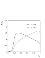
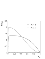
Figure 1: Energy spectra of the $\tau$ decay products $\pi$, $\rho$, e and $\mu$, respectively.

The sensitivity to ${\cal P}_{\tau}$ for a given channel depends on the relative shape of $h_{0}$ and $h_{1}$ and is maximal for the $\tau\rightarrow\pi\nu$ channel (figure 1). In the case of multi–pion $\tau$ decays, as $\tau\rightarrow\rho\nu$ and $\tau\rightarrow\rm\!a_{1}\nu$, this sensitivity can be substantially improved by defining an optimal variable ($\omega$) [7] or set of variables ($\cos\theta^{\ast},\ \cos\psi^{\ast}$) [4] which exploit the kinematics of the $\rm n\pi$ system in the final state. Different experiments [8, 9, 10, 11] use different approaches to the problem.

The $\tau$ longitudinal polarisation (${\cal P}_{\tau}$) value is extracted, for a given $\cos\theta$ range, by performing a fit of the distribution (6) to the data, once the detector and selection effects have been properly included in the $h_{0}$ and $h_{1}$ functions (by using Monte Carlo simulation and/or analytical techniques [6]). The data spectra (OPAL [8]) obtained in the whole $\cos\theta$ range of the detector for the e, $\mu$, ${\pi/\rm K}$ and ${\rm a_{\scriptscriptstyle{1}}}$ channels are shown in figure 2, together with the fit result.

Figure 2: Data spectra (OPAL) for the $\tau$ decay channels e, $\mu$, ${\pi/\rm K}$ and ${\rm a_{\scriptscriptstyle{1}}}$. The dots correspond to data and the solid line to the fit result. The dotted and dashed lines are the contribution from the negative and positive helicity spectra.

As an example, the two–dimensional distribution ($\cos\theta_{\rho}^{\ast}$, $\cos\psi_{\rho}^{\ast}$) for the L3 data [9] is shown in figure 3.

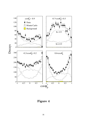
Figure 3: Data spectra from the L3 experiment for the $\tau\rightarrow\rho\nu$ decay channel. The dots correspond to the data and the solid line to the fit result.

2.2 Data Sample Selection

The $\rm e^{+}e^{-}\rightarrow\tau^{+}\tau^{-}$ processes are characterised for being low multiplicity events, with different particle signatures in opposite hemispheres (in most of cases). In addition, the invariant mass of the event is well below the Z mass, due to the presence of undetected neutrinos. The main background to this process is coming from $\rm e^{+}e^{-}\rightarrow\rm e^{+}e^{-}$ and $\rm e^{+}e^{-}\rightarrow\mu^{+}\mu^{-}$ with misidentified particles in the final state, as well as from two photon events.

The experiments at LEP are well suited for identifying individual $\tau$ decay channels by considering the tracking chambers information, showers from the electromagnetic and hadron calorimeters and the information from the muon chambers. In general the identification efficiencies are high, except for multi–pion final states in which ${\pi^{\scriptscriptstyle{0}}}$ identification plays a crucial role. As a consequence, background in the hadronic $\tau$ decay channels comes mainly from misidentification of other hadronic channels. In table 1 we can see the efficiencies and background contribution for the different $\tau$ decays. More details about selection and identification criteria can be found in [8, 9, 10, 11].

Table 1: Efficiencies (upper line) and background (lower) for the different experiments data samples.

	e	$\mu$	$\pi$	$\rho$	${\rm a_{\scriptscriptstyle{1}}}$	#decays
ALEPH	59	82	71	59	59	52 K
	2	4	7	9	9
DELPHI	92	87	60	45	60	71 K
	5	3	10	15	15	(49 K)
OPAL	96	87	83	70	66	123 K
	3	2	19	27	25
L3	76	70	72	70	33	111 K
	5	5	15	11	28

For the analysis the DELPHI, OPAL and L3 Collaborations have used the data collected between 1990 and 1994, while ALEPH used data collected up to 1992. ALEPH and OPAL results are final. Those from DELPHI and L3 are preliminary.

2.3 Results from ${\cal P}_{\tau}$

Following the procedure described in section 2.1, the $\tau$ longitudinal polarisation is measured for different values of $\cos\theta$ (figure 4, DELPHI [10]).

Figure 4: Tau longitudinal polarisation measurement as a function of $\cos\theta$. The dots correspond to the data and the solid line to the fit result.

The values of ${\cal A}_{\tau}$ and ${\cal A}_{e}$ are obtained by fitting the expression (3) —which is corrected for initial state radiation, $\gamma$ exchange and $\gamma$–Z interference— to the distribution ${\cal P}_{\tau}(\cos\theta)$ in data. The results of these measurements from the four LEP experiments are shown in figure 5.

The main sources of systematic errors come from effects distorting the shape of the spectra, namely the calibration of the different detectors and the energy dependence of the identification efficiency, specially in the channels involving $n\,{\pi^{\scriptscriptstyle{0}}}$.

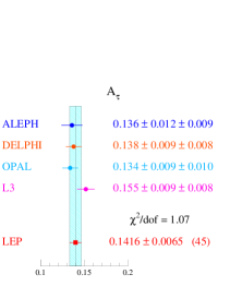
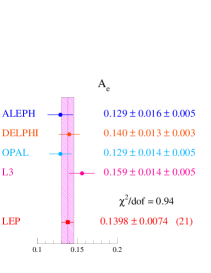
Figure 5: LEP results on ${\cal A}_{\tau}$ and ${\cal A}_{e}$.

The average LEP result for ${\cal A}_{\tau}$ and ${\cal A}_{e}$ is:

$$\qquad{\cal A}_{\tau}\ = \ 0.1401\pm 0.0067$$

$$\qquad{\cal A}_{e}\ = \ 0.1382\pm 0.0076$$

These results are consistent with the of lepton universality of the neutral currents. Under this assumption ${\cal A}_{e-\tau}$ has been calculated to be:

$$\qquad{\cal A}_{e-\tau}\ =\ 0.1393\pm 0.0050$$

which gives the following value of the weak mixing angle (equation 4):

$$\qquad\sin^{2}\theta_{W}\ =\ 0.2325\pm 0.0006$$

This result is in agreement with other LEP results [12].

3 TRANSVERSE AND NORMAL SPIN CORRELATIONS

The study of spin correlations has a special interest as it provides important additional tests of the Standard Model. A non vanishing correlation between the transverse and normal components of both taus spins in $\rm e^{+}e^{-}\rightarrow\tau^{+}\tau^{-}$ processes gives rise to terms in the cross section in equation (1) proportional to $C_{2}$ and $D_{2}$. The transverse–transverse (${\rm C_{TT}}$) and transverse–normal (${\rm C_{TN}}$) spin correlations are defined as:

$${\rm C_{TT}}\ \equiv\ \ \ {C_{2}\over C_{0}}\ = \ {|a_{\tau}|^{2}-|v_{\tau}|^{2}\over|a_{\tau}|^{2}+|v_{\tau}|^{2}}$$ (7)

$${\rm C_{TN}}\ \equiv\ \ \ {D_{2}\over C_{0}}\ = \ -{2\,\Im(v_{\tau}\,a_{\tau}^{\ast})\over|a_{\tau}|^{2}+|v_{\tau}|^{2}}$$ (8)

As it can be seen from this definition, ${\rm C_{TT}}$ is not symmetric in $a_{\tau}$ and $v_{\tau}$: a value of ${\rm C_{TT}}$ different from one would point to a Lorentz structure of the neutral currents which is different from the Standard Model. In particular, a negative value would reveal the dominance of the vector coupling in the neutral $\tau$ current. Moreover, ${\rm C_{TN}}$ is a CP–odd observable: a value of ${\rm C_{TN}}$ different from zero (the SM prediction) would indicate CP violation in weak interactions.

3.1 Experimental Determination

The determination of the spin correlations makes use of the kinematics of both $\tau$ decay products in the event. In this section, some idea on the analysis method will be given. A detailed description of the different methods and results can be found in [13, 14, 15].

Let us consider the process $\rm e^{+}e^{-}\rightarrow\tau^{+}\tau^{-}\rightarrow X_{1}^{-}X_{2}^{+}+n\nu$ and let us define a reference system such that $X_{1}^{-}$ goes along the z–axis and $X_{2}^{+}$ lies in the xz–plane. If we denote by $\Phi$ the azimuthal angle of the incident electron in this reference system, the $\Phi$ spectrum for a given final state can be written, from the cross section in equation (1), as a function of ${\rm C_{TT}}$ and ${\rm C_{TN}}$:

$$\frac{d\sigma}{d\Phi}\ \propto\ {\rm C_{TT}}\cos(2\Phi)+{\rm C_{TN}}\sin(2\Phi)$$ (9)

The values of ${\rm C_{TT}}$ and ${\rm C_{TN}}$ are obtained by performing a likelihood fit of this function to the $\Phi$ distribution in the data. Figure 6 shows the $\Phi$ variable spectrum obtained from data (ALEPH [13]) for the different $\tau^{+}\tau^{-}$ final states (dots) together with the theoretical distribution (line). The sensitivity to ${\rm C_{TT}}$ and ${\rm C_{TN}}$ is higher for final states involving $\tau\rightarrow\pi\nu$ and lower for the leptonic $\tau$ decays.

The main sources of systematic errors are the internal alignment of the subdetectors and the background due to misidentification of $\tau^{+}\tau^{-}$ final states.

Figure 6: $\Phi$ distribution for the different $\tau^{+}\tau^{-}$ final states (ALEPH).

3.2 $\bf{\rm C_{TT}}$ and $\bf{\rm C_{TN}}$ Results

The analysis of the spin correlations is based in a data sample of about 37000 $\tau^{+}\tau^{-}$ events collected in the period 1992–94 by the ALEPH [13], DELPHI [14] and L3 [15] Collaborations.

The results from the corresponding analyses is summarised in table 2, including the LEP average. The Standard Model predictions are in agreement with these results.

Table 2: LEP results on ${\rm C_{TT}}$ and ${\rm C_{TN}}$.

	${\rm C_{TT}}$	${\rm C_{TN}}$
Aleph	$1.00\pm 0.14\pm 0.04$	$-0.08\pm 0.14\pm 0.02$
Delphi	$0.87\pm 0.20\pm 0.12$	—
L3	$1.04\pm 0.26\pm 0.06$	$0.36\pm 0.26\pm 0.05$
LEP	$0.98\pm 0.11$	$0.02\pm 0.13$

References

-
[1]
S.L. Glashow, Nucl. Phys. A 22 (1961) 579;
S. Weinberg, Phys. Rev. Lett. 19 (1967) 1264;
A. Salam, “Elementary Particle Theory”, Ed. N. Svartholm, Stockholm, “Almquist and Wiksell” (1968), 367 - [2] J. Bernabeu et al., Phys. Lett. B 257 (1991) 219
- [3] S. Jadach, Z. Was et al., in “Z Physics at LEP 1”, Vol. 1, p. 235 and references therein CERN Report CERN 89–08 (1989), Eds. G. Altarelli, R. Kleiss and C. Verzegnassi
- [4] K. Hagiwara, A. D. Martin and D. Zeppenfeld, Phys. Lett. B 235 (1990) 198
- [5] A. Rougé, Z. Phys. C48 (1990) 75
- [6] P. García–Abia, Informes Técnicos del CIEMAT 783 (1996) 1, “Ph.D. Thesis”
- [7] M. Davier et al., Phys. Lett. B 306 (1993) 411
- [8] OPAL Collaboration, G. Alexander et al., Z. Phys. C72 (1996) 365
- [9] L3 Collaboration, ICHEP–96 (Warsaw), PA07–056 (1996)
- [10] DELPHI Collaboration, ICHEP–96 (Warsaw), PA07–008 (1996)
- [11] ALEPH Collaboration, D. Buskulic et al., Preprint CERN–PPE/95–023
- [12] Christoph Schäfer, San Miniato proceedings (1997), “The Z Lineshape at LEP”
- [13] ALEPH Collaboration, R. Barate et al., Preprint CERN–PPE/97–047
- [14] DELPHI Collaboration, P. Abreu et al., Preprint CERN–PPE/97–034 (1997)
- [15] R. Völkert, “A full Spin Analysis of the Process using the L3 Detector at LEP”, Ph.D. Thesis (1997) Huboldt Universität zu Berlin