DØ Results on $W$ Boson Properties

Abstract

The DØ experiment collected $\approx 15~{}\rm{pb^{-1}}$ in run 1A (1992-1993) and $\approx 89~{}\rm{pb^{-1}}$ in run 1B (1994-1995) of the Fermilab Tevatron Collider using $p\bar{p}$ collisions at $\sqrt{s}=1.8~{}\rm{TeV}$. Results from analyses of events with $W$ and $Z$ bosons are presented for the run 1B data samples. From $W\rightarrow e\nu,\mu\nu$ and $Z\rightarrow ee,\mu\mu$ decays, the $W$ and $Z$ production cross sections and the $W$ width are determined. Events with $W\rightarrow\tau\nu$ decays are used to determine the ratio of the electroweak gauge coupling constants as a measure of lepton universality. Using $W\rightarrow e\nu$ and $Z\rightarrow ee$ decays, the $W$ boson mass is measured.

I Introduction

The DØ experiment collected $\approx 15~{}\rm{pb^{-1}}$ in run 1A (1992-1993) and $\approx 89~{}\rm{pb^{-1}}$ in run 1B (1994-1995) of the Fermilab Tevatron Collider using $p\bar{p}$ collisions at $\sqrt{s}=1.8~{}\rm{TeV}$. Results are presented from data collected by the DØ experiment that test the Standard Model (SM) of electroweak interactions[1]. Measurements of the $W$ and $Z$ boson production cross sections, the $W$ decay width, the ratio of the gauge coupling constants, and the $W$ mass are presented.

II The DØ Detector

The DØ detector was designed to study a variety of high transverse momentum ($p_{T}$) physics topics and has been described in detail elsewhere [2]. It does not have a central magnetic field, making possible a compact, hermetic detector with almost full solid angle coverage. The detector has an inner tracking system which measures charged tracks to a pseudo-rapidity $\eta<3.2$, where $\eta=-\ln\tan{\theta\over 2}$ and $\theta$ is the polar angle. The tracking system is surrounded by finely-segmented uranium liquid-argon calorimeters (one central and two end-caps). Surrounding the calorimeter is a muon magnetic spectrometer which consists of magnetized iron toroids that are situated between the first two of three layers of proportional drift tubes.

Electrons and photons were identified by the shape of their energy deposition in the calorimeter and a matching track (for electrons). The energy ($E$) was measured by the calorimeter with a resolution of $\approx 15\%/\sqrt{E}~{}{\rm(GeV)}$. Neutrinos were not identified in the detector but their transverse momentum was inferred from the missing transverse energy in the event: ${\hbox{$\vec{E}$\kern-6.00006pt\lower-0.43057pt\hbox{/}}}_{T}~{}$$=-\sum_{i}E_{i}\sin\theta$, where the sum $i$ extends over all cells in the calorimeter. Muons were identified by a track in the muon chambers matched with a track in the central tracking chambers.

III $W$ and $Z$ Production

Events in which a $W$ or $Z$ boson is produced are used to measure the cross section times branching fraction, the $W$ width and the ratio of the gauge couplings. In these analyses, the $W$ and $Z$ gauge bosons are identified through their leptonic decay modes: $W\rightarrow e\nu,\mu\nu,\tau\nu$ and $Z\rightarrow ee,\mu\mu$. These modes have a cleaner signature and are easier to distinguish from the background of QCD multijet production than hadronic decay modes. The events with decays into $e$’s and $\mu$’s are selected by requiring a high-$p_{T}$ $e$ or $\mu$ and large ${\hbox{$E$\kern-6.00006pt\lower-0.43057pt\hbox{/}}}_{T}~{}$for $W$’s and two high-$p_{T}$ $e$’s or $\mu$’s for $Z$’s. The hadronic decay of the $\tau$ is used to to select the $W\rightarrow\tau\nu$ events.

A Production Cross Sections

The measurement of the product of the cross section and the branching fraction for $W$’s and $Z$’s provides a fundamental test of the Standard Model. These measurements have been published for the run 1A data sample[3] and the preliminary results are presented here for the run 1B data sample.

For the final event selection in this analysis, electrons were restricted to a region $|\eta|<1.1$ and $1.5<|\eta|<2.5$ and muons to a region $|\eta|<1.0$. The $W\rightarrow e\nu$ events were selected by requiring the transverse energy of the electron $E_{T}>25~{}\rm{GeV}$ and ${\hbox{$E$\kern-6.00006pt\lower-0.43057pt\hbox{/}}}_{T}~{}$$>25~{}\rm{GeV}$ and the $Z\rightarrow ee$ events were required to have two $e$’s with $E_{T}>25~{}\rm{GeV}$. The $W\rightarrow\mu\nu$ event selection required $p_{T}(\mu)>20~{}\rm{GeV},$ and ${\hbox{$E$\kern-6.00006pt\lower-0.43057pt\hbox{/}}}_{T}~{}$$>20~{}\rm{GeV}$ and the $Z\rightarrow\mu\mu$ selection required $p_{T}>15,20~{}\rm{GeV}$ for the two $\mu$’s. The transverse mass for $W$ events and invariant mass for $Z$ events in the final data samples are shown in Fig. 1. Table I gives the number of events observed, the acceptance, the efficiency, the background and the luminosity for these data samples.

FIG. 1.: Transverse and invariant mass distributions for the $W\rightarrow e\nu,\mu\nu$ and $Z\rightarrow ee,\mu\mu$ run 1B data samples.

	Electron	Muon
# $W$ candidates	59579	4472
Acceptance $(\%)$	$43.4\pm 1.5$	$20.1\pm 0.7$
$\epsilon_{W}(\%)$	$70.0\pm 1.2$	$24.7\pm 1.5$
Background$(\%)$	$8.1\pm 0.9$	$18.6\pm 2.0$
Luminosity $(pb^{-1})$	$75.9\pm 6.4$	$32.0\pm 2.7$
# $Z$ candidates	5702	173
$A_{Z}(\%)$	$34.2\pm 0.5$	$5.7\pm 0.5$
$\epsilon_{Z}(\%)$	$75.9\pm 1.2$	$43.2\pm 3.0$
Bkg.$(\%)$	$4.8\pm 0.5$	$8.0\pm 2.1$
Lum. $(pb^{-1})$	$89.1\pm 7.5$	$32.0\pm 2.7$

TABLE I.: The quantities used to measure the preliminary cross sections for $W\rightarrow e\nu,\mu\nu$ and $Z\rightarrow ee,\mu\mu$ for the run 1B data sample.

The preliminary measurements of the cross section times branching fraction ($\sigma\cdot B$) are given in table II and are shown in Fig. 2 along with the results from CDF[4]. The $\tau$ results shown will be discussed in section III C. Also shown in Fig. 2 are comparisons of $\sigma\cdot B$ with SM predictions[5]. The predictions use the CTEQ2M parton distribution functions (pdf)[6].

FIG. 2.: Tevatron measurements for the cross sections times branching ratios for $W\rightarrow e\nu,\mu\nu,\tau\nu$ and $Z\rightarrow ee,\mu\mu$ compared to SM predictions.

$\sigma_{W}\cdot B(W\rightarrow e\nu)$	=	2.38	$\pm$ 0.01	$\pm$ 0.09	$\pm$ 0.20 nb
$\sigma_{W}\cdot B(W\rightarrow\mu\nu)$	=	2.32	$\pm$ 0.04	$\pm$ 0.16	$\pm$ 0.19 nb
$\sigma_{Z}\cdot B(Z\rightarrow ee)$	=	0.235	$\pm$ 0.003	$\pm$ 0.005	$\pm$ 0.020 nb
$\sigma_{Z}\cdot B(Z\rightarrow\mu\mu)$	=	0.202	$\pm$ 0.016	$\pm$ 0.020	$\pm$ 0.017 nb
			$(\pm{\rm stat})$	$(\pm{\rm syst})$	$(\pm{\rm lum})$

TABLE II.: The preliminary cross sections for $W\rightarrow e\nu,\mu\nu$ and $Z\rightarrow ee,\mu\mu$.

B $W$ width

The ratio of the $W$ and $Z$ production cross sections can be used to measure the leptonic branching ratio $B(W\rightarrow l\nu)$ and extract the $W$ width ($\Gamma_{W}$). From the measured width, a limit may be placed on unexpected decay modes of the $W$. Many common systematic errors, including the luminosity error, cancel in the leptonic branching ratio:

$$R={{\sigma_{W}\cdot B(W\rightarrow l\nu)}\over{\sigma_{Z}\cdot B(Z\rightarrow ll)}}={{\sigma_{W}}\over{\sigma_{Z}}}{{\Gamma(W\rightarrow l\nu)}\over{\Gamma(Z\rightarrow ll)}}{{\Gamma_{Z}}\over{\Gamma_{W}}}.$$

Using the results above for $\sigma\cdot B$ and combining the electron and muon measurements, we obtain a preliminary run 1B result of $R=10.32\pm 0.43$. The leptonic branching fraction of the $W$ may then be calculated, $B(W\rightarrow l\nu)=B(Z\rightarrow ll)\cdot{{(\sigma_{Z}}/{\sigma_{W}})}\cdot R=(10.43\pm 0.44)\%$ using the measured value of $R$, the value of $B(Z\rightarrow ll)$ from LEP measurements[7] and $\sigma_{W}/\sigma_{Z}=3.33\pm 0.03$ from the SM prediction[8]. The total width of the W is then obtained from this measurement of $B(W\rightarrow l\nu)$ and the value of $\Gamma(W\rightarrow l\nu)$ from SM predictions[9]. The preliminary run 1B measurement is

$$\Gamma_{W}=2.159\pm 0.092~{}\rm{GeV}.$$

Comparison of the published world average $\Gamma_{W}=2.062\pm 0.059~{}\rm{GeV}$[3] (does not include the run 1B measurement) with the SM prediction $\Gamma_{W}=2.077\pm 0.014~{}\rm{GeV}$[9], gives a $95\%$ confidence level upper limit of $\Delta\Gamma_{W}<109~{}\rm{MeV}$ on unexpected (non-SM) decays of the $W$.

C Measurement of the Ratio of the Couplings

The decay $W\rightarrow\tau\nu$ is studied as a test of lepton universality by measuring the ratio of the electroweak coupling constants $g_{\tau}^{W}/g_{e}^{W}$. The $\tau$ events are obtained from a sample in which inelastic collisions were selected by requiring a single interaction signature from the Level 0 trigger. The integrated luminosity for the $\tau$ trigger used in this analysis is $16.8\pm 0.9~{}{\rm pb^{-1}}$.

To select the $W\rightarrow\tau\nu$ events from the $W$ data sample, the hadronic decay of the $\tau$ is used. These events are identified by the presence of an isolated, narrow jet. Jets were reconstructed using a cone algorithm with radius $0.7$ in $\eta-\phi$ space and the width of the jet was required to be $rms_{jet}<0.25$. The requirements that $E_{T}$(jet)$>25$ GeV, ($|\eta|<0.9$), $\mbox{${\hbox{$E$\kern-6.00006pt\lower-0.43057pt\hbox{/}}}_{T}~{}$}>25$ GeV and that there be no opposite jet were placed on the data sample. In order to separate the events with a jet from a $\tau$ decay from the large background of QCD jets, the profile distribution of the jets is used. The profile is defined as the sum of the highest two tower $E_{T}$’s divided by the cluster $E_{T}$. The profile distributions from the $\tau$ sample and the QCD background sample (selected from events with low ${\hbox{$E$\kern-6.00006pt\lower-0.43057pt\hbox{/}}}_{T}~{}$) are shown in Fig. 3. A requirement that the profile variable be $>0.55$ is made to select the final $\tau$ event sample. The shaded low-profile region in Fig. 3a is used to estimate the remaining QCD background.

FIG. 3.: The distribution of the profile quantity for the $\tau$ candidate sample and for the QCD background sample.

The number of signal events contained in the final data sample is listed in table III along with the estimated background contributions. The preliminary value of the cross section times branching ratio is $\sigma\cdot B(W\to\tau\nu)=2.38\pm 0.09(stat)\pm 0.10(syst)~{}{\rm nb}$ where the error due to the luminosity has not been included. Comparing this value with the measurement of $\sigma\cdot B(W\to e\nu)$ from run 1A[3], the ratio of the couplings is determined $g_{\tau}^{W}/g_{e}^{W}=1.004\pm 0.019(stat)\pm 0.026(syst)$. This measurement shows good agreement with $e-\tau$ universality at high energy.

	Number of Events
Final Data Sample	1202
QCD Background	$106\pm 7\pm 5$
Noise Events	$81\pm 14$
$Z\to\tau\tau$	$32\pm 5$
$W\to e\nu$	$3\pm 1$

TABLE III.: The quantities used to measure the run 1B preliminary cross section for $W\rightarrow\tau\nu$.

IV $W$ Mass

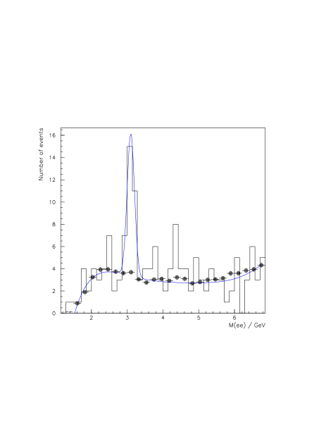
FIG. 4.: The invariant mass distributions are shown for (a) $\pi^{0}\rightarrow\gamma\gamma\rightarrow e^{+}e^{-}e^{+}e^{-}$ events (points), (b) $J/\psi\rightarrow ee$ events (points), and (c) $Z\rightarrow ee$ events (points), compared to Monte Carlo simulations (line). (d) Constraints on $\alpha$ and $\delta$ from $Z\rightarrow ee$ decays (large ellipse), $J/\psi\rightarrow ee$ decays (wide band), $\pi^{0}\rightarrow\gamma\gamma\rightarrow e^{+}e^{-}e^{+}e^{-}$ decays (narrow band), and for all three combined (small ellipse).

The electroweak Standard Model can be specified by three parameters. These may be taken to be $\alpha$, $G_{F}$ and $M_{Z}$, all measured to $<0.01\%$. At lowest order, the $W$ mass is precisely defined as $M_{W}=A/\sin\theta_{W}$ with $\sin^{2}\theta_{W}=1-M_{W}^{2}/M_{Z}^{2}$, where $\theta_{W}$ is the weak mixing angle and $A=(\pi\alpha/\sqrt{2}G_{F})^{1/2}$. The current data are sufficiently precise to require comparison to theoretical predictions which include higher order corrections. These corrections have contributions due to the running of $\alpha\rightarrow\alpha(M_{Z}^{2})$ and to loop diagrams which introduce a dependence on the square of the top quark mass, $m_{top}$, and the log of the Higgs mass, $M_{H}$. A precision measurement of the $W$ mass therefore defines the size of the radiative corrections in the SM and along with $m_{top}$ it can constrain $M_{H}$. A direct measurement also serves to test the consistency of the SM.

FIG. 5.: (a) Comparison of the $u_{\parallel}$ distribution from $W\rightarrow e\nu$ events (points) and the MC simulation (histogram); (b) Comparison of the angle between the recoil and the electron in the transverse plane from $W\rightarrow e\nu$ events (points) and the MC simulation (histogram).

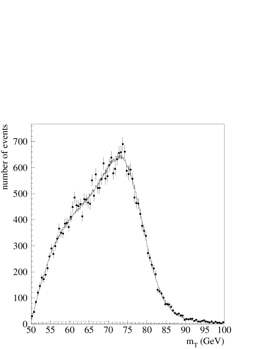
FIG. 6.: (a) The transverse mass distribution, (b) the electron transverse momentum distribution, and (c) the neutrino transverse momentum distribution are shown for $W$ events (points). The best fits of the MC simulation (histograms) are also shown.

Previous results from the run 1A data sample have been published[10] and yielded a value of $M_{W}=80.350\pm 0.270~{}{\rm GeV/c^{2}}$. In the analysis presented here, the preliminary measurement of $M_{W}$ from the run 1B data sample is presented, using a calorimeter-based measurement. The calorimeter is not calibrated independently to the precision needed and therefore the ratio of the $W$ to $Z$ masses was measured and then scaled to the precisely known ($<0.01\%$) $Z$ mass[11]. Many systematic errors cancel in this ratio.

Experimentally, the remnants of the interaction $p\bar{p}\rightarrow W(\rightarrow e\nu)+X$ are detected. Here $X$ is due to the recoil $(rec)$ to the $W$ plus the underlying event. The energy of the electron and the ${\hbox{$\vec{E}$\kern-6.00006pt\lower-0.43057pt\hbox{/}}}_{T}~{}$ were measured. The $\mbox{${\hbox{$\vec{E}$\kern-6.00006pt\lower-0.43057pt\hbox{/}}}_{T}~{}$}=-\vec{p}_{T}(rec)-\vec{p}_{T}(e)=\vec{p}_{T}(W)-\vec{p}_{T}(e)$ and is identified with the neutrino transverse momentum $\vec{p}_{T}(\nu)$ but differs from $\vec{p}_{T}(\nu)$ because of the presence of the underlying event.

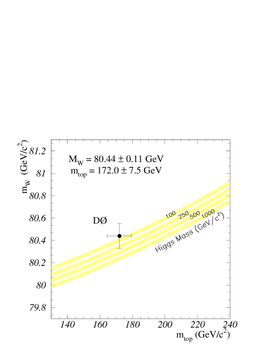
FIG. 7.: The DØ determination of the mass of the top quark is shown versus the measured $W$ mass. The SM prediction (see text) for various assumptions of the Higgs boson mass is indicated by the bands.

Because the longitudinal momentum of the $\nu$ is not measured, the $W$ invariant mass cannot be constructed. Instead the distribution in transverse mass $M_{T}(W)=\sqrt{2p_{T}(e)p_{T}(\nu)-2\vec{p}_{T}(e)\cdot\vec{p}_{T}(\nu)}$ is used to obtain the $W$ mass. For $Z$ decays, the energies of both electrons are measured and the invariant mass is reconstructed.

The $W\rightarrow e\nu$ events were selected by requiring an isolated electron with $E_{T}>25~{}\rm GeV$, $p_{T}(W)<15~{}\rm GeV/c$ and $\mbox{${\hbox{$E$\kern-6.00006pt\lower-0.43057pt\hbox{/}}}_{T}~{}$}>25~{}\rm GeV$. The $Z\rightarrow ee$ events were selected by requiring two isolated electrons each with $E_{T}>25~{}\rm GeV$, and $70<M_{Z}<110~{}{\rm GeV/c^{2}}$. Electrons were required to be in the region $|\eta|<1.0$. There were 28323 $W$ events and 2179 $Z$ events in this sample. The electron polar angle was determined from the shower centroid of the energy cluster in the electromagnetic (EM) calorimeter and the center-of-gravity of the corresponding track. The uncertainty in determining this angle results in an uncertainty of $\pm 28~{}\rm MeV/c^{2}$ in $M_{W}$.

The mass of the $W$ is determined by a maximum likelihood fit of the measured $M_{T}(W)$ distribution to Monte Carlo (MC) distributions which were generated for 21 different values of $M_{W}$ in $100~{}{\rm MeV}$ steps. This fast MC simulation uses a theoretical calculation for the $W$ production and decay and a parameterized model for the detector response. Kinematic cuts are placed on the MC quantities as done in the data. All the parameters in the MC are set by $Z$ data and other data samples. Below is a discussion of the determination of the parameters in the $W$ Monte Carlo. The $Z$ data are treated in an analagous fashion. Systematic errors are set using large statistics samples of MC data and varying the parameter within its errors and are discussed throughout.

The $W$ production is modelled by the double differential cross section in $p_{T}(W)$ and rapidity, $y$, calculated at next-to-leading order by Ladinsky and Yuan[12] and using the MRSA[13] pdf. The $W$ resonance is generated by a relativistic Breit-Wigner, incorporating the mass dependence of the parton momentum distribution:

$$\frac{d\sigma}{dm}\sim\frac{e^{-\beta\cdot m}}{m}\cdot\frac{m^{2}}{(m^{2}-M_{W}^{2})^{2}+\frac{m^{4}\Gamma^{2}}{M_{W}^{2}}}.$$ (1)

The angular decay products are generated at ${\cal O}(\alpha_{s})$, allowing $p_{T}(W)>0$, in the $W$ rest frame. This angular decay is of the form[14]

$${{d\sigma}\over{d\cos\theta}}\sim(1+\alpha_{1}\cos\theta+\alpha_{2}\cos^{2}\theta)$$

where $\alpha_{1,2}=\alpha_{1,2}(p_{T}(W))$[14]. Radiative decays ($W\rightarrow e\nu\gamma$) are generated according to Berends and Kleiss[15]. Events in which $W\rightarrow\tau\nu\rightarrow e\nu{\bar{\nu}}\nu$ are indistinguishable from $W\rightarrow e\nu$ decays and are therefore modelled in the simulation, including the polarization of the $\tau$ in the decay angular distribution. The decay products are then boosted to the laboratory frame. At this point, the values of $p_{T}(e)$ and $p_{T}(W)$ have been generated and $p_{T}(\nu)$ is calculated. The effects of the detector and underlying event are now modelled.

The EM (electron) calorimeter energy scale of the calorimeter was determined using $J/\psi\rightarrow ee$, $\pi^{0}\rightarrow\gamma\gamma\rightarrow e^{+}e^{-}e^{+}e^{-}$, and $Z\rightarrow ee$ events. From test beam studies, it was determined that a linear relationship between the true and measured energies could be assumed: $E_{\rm meas}=\alpha E_{\rm true}+\delta$. This gives a relation $M_{meas}=\alpha M_{true}+\delta f$ between the measured and true mass values, keeping terms to first order in $\delta$ only. The variable $f={2(E_{1}+E_{2})\over M}\sin^{2}{\gamma\over 2}$ depends on the event decay topology. Since the ratio of $M_{W}$ to $M_{Z}$ is actually measured, one finds

$$\left({M_{W}\over{M_{Z}}}\right)^{meas}=\left({M_{W}\over{M_{Z}}}\right)^{true}\left[1+{f\delta\over\alpha}\cdot{(M_{Z}-M_{W})\over{M_{W}M_{Z}}}\right].$$

We note that to first order the measured ratio is insensitive to the EM energy scale, if $\delta$ is small, and that the error on the measured ratio due to the uncertainty in $\delta$ is suppressed.

Figure 4 shows the mass spectra for the $\pi^{0},J/\psi$ and $Z$ data samples. The allowed ranges for $\alpha$ and $\delta$ are shown in Fig. 4d for each data sample. The overlap region is the $1\sigma$ contour from all three data samples. The scale $\alpha$ is fixed by the $Z$ data. The value of $\delta$ is constrained by the $J/\psi$ and $\pi^{0}$ data, essentially independent of $\alpha$. Allowing a quadratic term in the energy response, to account for nonlinear responses at low energies as measured at the test beam, leads to the systematic error on $\delta$. The allowed values determined for $\alpha$ and $\delta$ are $\alpha=0.95329\pm 0.00077$ and $\delta=-0.160\pm 0.016(stat.)^{~{}+.060}_{~{}-.210}(syst.)~{}\rm GeV$. The error in the EM energy scale introduces an uncertainty in $M_{W}$ of $\pm 65{\rm~{}MeV/c^{2}}$ and is dominated by the statistical error in determining the $Z$ mass.

The EM energy resolution is parameterized as ${\sigma/E}=\sqrt{C^{2}+({S/{\sqrt{E_{T}}}})^{2}+({N/E})^{2}}$ for the central calorimeter. Test beam data are used to set the sampling term, $S=0.13~{}\rm{(GeV^{1/2})}$, and the noise term, $N=0.4~{}\rm{GeV}$. By constraining the width of the $Z$ invariant mass distribution in the MC to that from the data, the constant term is set to $C=(1.15~{}{{}^{+0.27}_{-0.36}})$. The uncertainty in the energy resolution leads to an uncertainty of $\pm 23~{}\rm MeV/c^{2}$ in $M_{W}$.

The hadronic (recoil) energy scale of the calorimeter is determined relative to the EM energy scale by using $Z$ events and measuring the transverse momenta of the $Z$ from both the recoil or the two electrons. The $p_{T}{\rm-balance}$ is constructed:

$$p_{T}{\rm-balance}\equiv[\vec{p}_{T}(ee)+\vec{p}_{T}(rec)]\cdot{\hat{\eta}}$$

where $\hat{\eta}$ is defined as the bisector of the two electrons. From studies using HERWIG[16] and GEANT[17], it was determined that the recoil response could be written as a function of the EM response: $p_{T}(rec)={\cal R}_{rec}p_{T}(ee)$ with ${\cal R}_{rec}=\alpha_{rec}+\beta_{rec}{\rm log}~{}p_{T}(W)$. To ensure an equivalent event topology, $Z$ events in which one electron is in the forward region are included in this study. Comparing data to MC in a plot of $p_{T}{\rm-balance}$ versus $\vec{p}_{T}(ee)\cdot{\hat{\eta}}$, the recoil response parameters are determined to be $\alpha_{rec}=0.69\pm 0.06$ and $\beta_{rec}=0.04\pm 0.02$. The uncertainty in the recoil scale leads to an uncertainty of $\pm 23~{}\rm{MeV/c^{2}}$ in $M_{W}$.

The recoil (hadronic) energy resolution is determined by modelling both components of the recoil to the $W$: $\vec{p}_{T}(rec)^{meas}={{\cal R}_{rec}}\vec{p}_{T}(rec)+\alpha_{mb}\cdot\vec{U}_{mb}(tot)-U(\hat{e})$. The first component is the “hard” component due to the initial $p_{T}$ of the boson. It is smeared using a Gaussian of width $\sigma_{rec}=s_{rec}\sqrt{p_{T}(rec)}$. The second component is the “soft” component due to the underlying event and is modelled by a minimum-bias event obtained from the data. In selecting the minimum-bias events to use, the luminosity distribution of the $W$ event sample is modelled. The quantity $\vec{U}_{mb}$ is the total $\vec{E}_{T}$ of minimum-bias event and $\alpha_{mb}$ is a scale factor. The amount of underlying event in the electron direction, $U(\hat{e})$, is subtracted from the recoil and added onto the electron momentum. Using the width of the $p_{T}{\rm-balance}$ distribution (to which the energy calibration has been applied), the values of $s_{rec}$ and $\alpha_{mb}$ are constrained. The measured values are $s_{rec}=0.49\pm 0.14$ and $\alpha_{mb}=1.03\pm 0.03$ and their errors and lead to an uncertainty of of $\pm 33~{}\rm{MeV/c^{2}}$ in $M_{W}$.

Selection biases due to radiative decays and the amount of recoil energy in the electron direction and trigger efficiences are modelled in the MC simulation. The uncertainty in $M_{W}$ due to the modelling of these efficiencies and biases is negligible in the fit to the $M_{T}(W)$ spectrum.

Backgrounds to the $W$ event sample are included in the fitting procedure by including the shape and fraction of background events. The largest source of background in the $W$ sample is due to QCD multijet production in which there is a jet is mis-identified as an electron and ${\hbox{$E$\kern-6.00006pt\lower-0.43057pt\hbox{/}}}_{T}~{}$ due to energy fluctuations. This background contributes $1.4\pm 0.2\%$ to the $W$ sample. The other background considered is $Z\rightarrow ee$ events where one electron is not identified. This background contributes $0.33\pm 0.06\%$ to the $W$ sample. The uncertainty in size and shape of the backgrounds gives an uncertainty in $M_{W}$ of $\pm 12~{}\rm{MeV/c^{2}}$. All other sources of background are negligible.

The last systematic error to consider is that due to the modelling of the $W$ production. This uncertainty is due to the correlated uncertainties in the $p_{T}(W)$ spectrum and the pdf’s. There are three phenomenological parameters in the production model calculation ($g_{1},g_{2},g_{3}$)[12] and the largest sensitivity of the $p_{T}$ spectrum is to the $g_{2}$ parameter. To constrain the production model, the $g_{1}$ and $g_{3}$ parameters are fixed to their nominal values and the value of $g_{2}$ is constrained by the $p_{T}(Z)$ distribution from the data. Then the dependence of $M_{W}$ on the pdf used in the theoretical calculation is measured from the difference in $M_{W}$ from the nominal pdf (MRSA) as seen in Table IV. For each pdf, the theoretical calculation uses the value of $g_{2}$ constrained by the data for that case. The uncertainties on the measured $M_{W}$ due to the value of $g_{2}$ and the pdf used are $\pm 5~{}\rm{MeV/c^{2}}$ and $\pm 21~{}\rm{MeV/c^{2}}$, respectively. Errors on $M_{W}$ are also ascribed to uncertainties in the value of $\Gamma_{W}\rightarrow\pm$ 9 MeV, the parton luminosity parameter $\rightarrow\pm$ 10 MeV, and the modelling of radiative decays $\rightarrow\pm$ 20 MeV. The total uncertainty on $M_{W}$ due to the production model is $\sigma(M_{W})=\pm 34{\rm~{}MeV}$.

pdf	constrained $g_{2}$	$\Delta M_{W}~{}{\rm MeV}$
MRSA	$0.59$	-
MRSD-	$0.61$	+20
CTEQ3M	$0.54$	+5
CTEQ2M	$0.61$	-21

TABLE IV.: The variation of the measured $W$ mass when using different pdf’s in the production model. Each theoretical calculation uses the constrained value of $g_{2}$ for that pdf.

A measure of how accurately the MC describes the data is shown in Fig. 5. The quantity $u_{\parallel}=\vec{p}_{T}(rec)\cdot\hat{e}$, which is the hadronic energy in electron direction, is shown in Fig. 5a. A bias in $u_{\parallel}$ directly affects the $M_{T}(W)$ spectrum and it is also very sensitive to the recoil resolution. Another sensitive quantity is the difference in the azimuthal angle, $\Delta\phi$, between the electron and the recoil and is shown in Fig. 5b. Excellent agreement between the data and MC simulation is obtained.

Source	$\sigma_{M(W)}$ in $\rm{MeV/c^{2}}$
Statistical (W events)	69
Statistical (Z events)	65
Non-Uniform energy response ($\eta$)	10
Electron Angle Calibration	28
Electron Energy Resolution	23
Electron Energy Linearity	20
Electron Underlying Event	16
Hadronic Energy Scale	20
Hadronic Resolution	33
$P_{T}(W)$ Spectrum	5
pdf	21
parton luminosity	10
$W$ Width	9
Radiative Decays	20
QCD background	11
Z background	5
Systematic Total	70
Total	118

TABLE V.: Summary of errors on the $W$ mass measurement.

The $M_{T}(W)$ distribution from the data is shown in Fig. 6a together with the distribution from the best fit value of $M_{W}$ from the Monte Carlo simulation. The data are fit over a region $60$ to $90~{}\rm{GeV/c^{2}}$ and the preliminary value of the $W$ mass determined is $M_{W}=80.450\pm 0.070(stat.)\pm 0.065(scale)\pm 0.070(syst.)~{}{\rm GeV/c^{2}}$, giving a total error of $\pm 118~{}{\rm MeV/c^{2}}$. The errors on the $W$ mass are detailed in Table V.

As consistency checks, the $p_{T}(e)$ and $p_{T}(\nu)$ spectra are also fit to determine $M_{W}$ as shown in Figs. 6b and 6c. The fit to the $p_{T}(e)$ spectrum gives $M_{W}=80.49\pm 0.14~{}{\rm GeV/c^{2}}$ and the $p_{T}(\nu)$ fit gives $M_{W}=80.42\pm 0.18(stat.)~{}{\rm GeV/c^{2}}$ with the fitting region from $30$ to $50~{}\rm{GeV/c}$ in both cases.

In summary, the measured $W$ masses from the DØ data sample of $W\rightarrow e\nu$ decays with the $e$ in the central $\eta$ region are $M_{W}=80.35\pm 0.27~{}{\rm GeV/c^{2}}$ (run 1A) and $M_{W}=80.45\pm 0.12~{}{\rm GeV/c^{2}}$ (run 1B, preliminary). Combining these results and taking into account the correlated errors gives a DØ combined value of $M_{W}=80.44\pm 0.11~{}\rm{GeV/c^{2}}$.

Combining the new DØ result with other measurements[18, 19] from hadron collider experiments gives a new preliminary hadron collider average of $M_{W}=80.41\pm 0.09~{}\rm{GeV/c^{2}}$.

The constraints placed on the Higgs mass can be seen in Fig. 7, which shows the measured values of $M_{W}$ versus $m_{top}$[20] compared to the Standard Model prediction[21] for different values of the $M_{H}$ in the $m_{top}-M_{W}$ plane.

V Conclusions

In conclusion, DØ has collected $\approx 100{\rm pb}^{-1}$ of data from run 1 of the Tevatron and preliminary results on $W$ boson properties are found to be in agreement with the Standard Model. The $W$ and $Z$ cross sections are measured in the $e,\mu,\tau$ decay modes. The $W$ width is measured to be $\Gamma_{W}=2.159\pm 0.092~{}{\rm GeV}$. We confirm $e-\tau$ universality in $W$ decays with the measurement $g_{\tau}^{W}/g_{e}^{W}=1.004\pm 0.032$. The run 1 combined DØ $W$ mass, $M_{W}=80.44\pm 0.11~{}{\rm GeV/c^{2}}$, is currently the most accurate direct measurement.

REFERENCES

-
[1]
S. Weinberg, Phys. Rev. Lett. 19, 1264 (1967);
A. Salam, in Elementary Particle Theory, ed. by N. Svartholm (Almquist and Wiksell, Sweden, 1968), p. 367;
S.L. Glashow, J. Illiopoulos and L. Maiani, Phys. Rev. D 2, 1285 (1970). - [2] S. Abachi et al., (DØ Collaboration), Nucl. Instrum. Methods A338, 185 (1994).
- [3] S. Abachi et al., (DØ Collaboration), Phys. Rev. Lett. 75, 1456 (1995) and references therein.
- [4] F. Abe et al., (CDF Collaboration), Phys. Rev. Lett 76, 3070 (1996).
- [5] H. Hamberg, W.L. van Neerven and T. Matsuura, Nucl. Phys. B 359, 343 (1991); W.L. van Neerven and E.B. Zijlstra, Nucl. Phys. B bf 382, 11 91992).
- [6] H.L. Lai et al., Phys. Rev. D51, 4763 (1995).
- [7] Particle Data Group, L. Montanet et al., Phys. Rev. D50 1173 (1994).
- [8] We use ref. [5] with the CTEQ2M pdf, GeV, GeV and .
- [9] J.L. Rosner, M.P. Worah and T. Takeuchi, Phys. Rev. D49, 1363 (1994) with GeV.
- [10] S. Abachi et al., (DØ Collaboration), Phys. Rev. Lett. 77, 3309 (1996).
- [11] CERN-PPE/95-172, LEP Electroweak Working Group, 1995.
- [12] G. Ladinsky, C.P. Yuan, Phys. Rev. D50, 4239 (1994).
- [13] A.D. Martin, R.G. Roberts and W.J. Stirling, Phys. Rev. D50, 6734 (1994) and A.D. Martin, R.G. Roberts and W.J. Stirling, Phys. Rev. D51, 4756 (1995).
- [14] E. Mirkes, Nucl. Phys. B 387, (1992) 3.
- [15] F. A. Berends and R. Kleiss, Z. Phys. C27, 365 (1985).
- [16] G. Marchesini and B.R. Webber, Nucl. Phys. B 310 (1988) 461.
- [17] F. Carminati et al., GEANT User’s Guide, CERN Program Library (Dec. 1991).
- [18] J. Alitti et al., (UA2 Collaboration), Phys. Lett., B276, 354 (1992).
- [19] F. Abe et al., (CDF Collaboration), Phys. Rev. Lett. 65, 2243 (1990); Phys. Rev. D43, 2070 (1991); Phys. Rev. Lett. 75, 11 (1995); Phys. Rev. D52, 4784 (1995).
- [20] S. Abachi et al., (DØ Collaboration), Phys. Rev. Lett. 74, 2632 (1995). See also “Direct Measurement of the Top Quark Mass”, S. Abachi et al., (the DØ Collaboration), FERMILAB-PUB-97/059-E, to be published in Phys. Rev. Lett. and “Measurement of the Top Quark Mass Using Dilepton Events”, B. Abbott et al., (DØ Collaboration), FERMILAB-PUB-97/172-E, Submitted to Phys. Rev. Lett.
- [21] ZFITTER: D. Bardin et al., Z. Phys. C44, 493 (1989); Comp. Phys. Comm. 59, 303 (1990); Nucl. Phys. B351, 1 (1991); Phys. Lett. B255, 290 (1991); and CERN-TH 6443/92 (May 1992).