The doubly Cabibbo-suppressed decay $D^{+}\to K^{+}\pi^{-}\pi^{+}$

Abstract

We report the observation of the doubly Cabibbo-suppressed decay $D^{+}\to K^{+}\pi^{-}\pi^{+}$ in data from Fermilab charm hadroproduction experiment E791. With a signal of 59 $\pm$ 13 events we measured the ratio of the branching fraction for this mode to that of the Cabibbo-favored decay $D^{+}\to K^{-}\pi^{+}\pi^{+}$ to be $B(D^{+}\to K^{+}\pi^{-}\pi^{+})$ / $B(D^{+}\to K^{-}\pi^{+}\pi^{+}$) $=$ ($7.7\pm 1.7\pm 0.8)\times 10^{-3}$. A Dalitz plot analysis was performed to search for resonant structures.

13.20Fc 14.40Lb 25.80Ls

The origin of the differences between the charm meson lifetimes is associated with their hadronic decays. While the semileptonic decay rates of the $D^{0}$ and $D^{+}$ are the same, the Cabibbo-favored (CF) hadronic decay rate of the $D^{0}$ is 3.2 times that of the $D^{+}$. There are at least two possible sources for this difference. The CF $D^{+}$ hadronic decay rate could be suppressed by destructive interference between spectator amplitudes containing indistinguishable final state quarks. It is also possible that the CF $D^{0}$ decay rate is enhanced by non-spectator amplitudes which do not exist for the $D^{+}$.

For both hadronic CF $D^{0}$ decays and doubly Cabibbo-suppressed (DCS) $D^{+}$ decays, all the final state quarks have different flavors, thus removing the possibility of destructive interference. In the simplest picture, non-spectator amplitudes are small enough to ignore, and one would expect $\Gamma_{DCS}(D^{+})/\Gamma_{CF}(D^{0})\approx\tan^{4}\theta_{C}$ and $\Gamma_{DCS}(D^{+})/\Gamma_{CF}(D^{+})\approx 3.2\times\tan^{4}\theta_{c}$. These relations need not be satisfied if non-spectator amplitudes are also important. Doubly Cabibbo-suppressed decays can thus provide important insights into the $D$ meson lifetime pattern.

In this paper we report a measurement from Fermilab experiment E791 of the branching fraction for the DCS decay $D^{+}\to K^{+}\pi^{-}\pi^{+}$. Throughout this paper, reference to $D^{+}$ and $D_{s}^{+}$ and to their decay modes imply also the corresponding charge-conjugate states.

The data were recorded from 500 GeV/$c$  $\pi^{-}$ interactions in five thin foils (one platinum, four diamond) separated by gaps of 1.34 to 1.39 cm. The experiment recorded $2\times 10^{10}$ events with a loose transverse energy trigger.

The E791 spectrometer was an upgraded version of the apparatus used in Fermilab experiments E516, E691, and E769 [1]. Position information for track and vertex reconstruction was provided by 23 silicon microstrip detectors (6 upstream of the target foils, 17 downstream), 10 proportional wire chamber planes (8 upstream and 2 downstream of the target) and 35 drift chamber planes. Momentum analysis was provided by two dipole magnets which bent particles in the horizontal plane. Particle identification was performed by two segmented threshold Čerenkov counters [2], allowing unambiguous identification of pions and kaons in the momentum range from 6 to 40 GeV/$c$.

After reconstruction, events with evidence of well-separated production (primary) and decay (secondary) vertices were retained for further analysis. The position resolutions along and transverse to the beam direction for the primary vertex were $350\,\mu$m and $6\,\mu$m, respectively. For 3-prong secondary vertices from $D^{+}$ decays, the transverse resolution was about $9\,\mu$m, nearly independent of the $D^{+}$ momentum; the longitudinal resolution was about 360 $\mu$m for a $D^{+}$ momentum of 70 GeV/$c$ and increased roughly linearly with a slope of $30\,\mu$m per 10 GeV/$c$.

We selected a generic $K\pi\pi$ sample containing both DCS $D^{+}\to K^{+}\pi^{-}\pi^{+}$ and CF $D^{+}\to K^{-}\pi^{+}\pi^{+}$ decay candidates. The abundant CF decay was used to determine the track and vertex selection criteria used in the search for the DCS decay. The criteria were chosen to maximize $N_{S}/\sqrt{N_{B}}$, where $N_{S}$ and $N_{B}$ are the numbers of signal and background events in the $K^{-}\pi^{+}\pi^{+}$ sample.

We required the secondary vertex to be well-separated from the primary vertex and located well outside the target foils and other solid material, the momentum vector of the candidate $D^{+}$ to point back to the primary vertex, and the decay track candidates to pass closer to the secondary vertex than to the primary vertex. We used longitudinal separations normalized by their resolutions to reduce momentum-dependent effects. Specifically, a 3-prong secondary vertex had to be separated by at least 20 $\sigma_{L}$ from the primary vertex and by at least 5 $\sigma_{L}$ from the closest material in the target foils, where the $\sigma_{L}$ are resolutions in the measured longitudinal separations. The sum of the momentum vectors of the three tracks from this secondary vertex could not miss the primary vertex by more than 40$\mu$m in the plane perpendicular to the beam. We formed the ratio of each track’s smallest distance from the secondary vertex to its smallest distance from the primary vertex, and required the product of these ratios for the three tracks to be less than 0.001.

In addition to the selection criteria described above, we required Čerenkov particle identification for all three decay candidate tracks. The Čerenkov efficiencies and corresponding misidentification rates were measured using the CF signal, in which the particle identification of the decay tracks can be determined from their charge. In this analysis the efficiency for correctly identifying kaons was 45%; the corresponding probability of misidentifiying real pions as kaons was 2%. Since misidentification of the odd-charged pion candidate was a large source of contamination, we used a more stringent identification criterion for this track than that for the like-charged pion. For the odd-charged pion, the efficiency for correct identification was 57%, and the probability of misidentifying kaons as pions was 13%. For the like-charged pion the efficiency for correct identification was 85%; the corresponding probability of misidentifying kaons as pions was 37%. The overall particle identification efficiency for $D^{+}\rightarrow K\pi\pi$ was 22%.

Due to particle misidentification and reconstruction errors, several other charm decays contributed to the background in the $K^{+}\pi^{-}\pi^{+}$ sample. The major sources of charm background are listed below.

a) $D^{+}$ and $D_{s}$ decays with missing neutrals, such as $D^{+}\to~{}\bar{K}^{*0}l^{+}\nu$, $D^{+}\to K^{-}\pi^{+}\pi^{+}\pi^{0}$ and $D_{s}\to\phi l^{+}\nu$. In these cases 4-body decays produced 3-prong vertices. Monte Carlo simulations showed that, because of particle misidentification, these events are spread smoothly across the entire $K^{+}\pi^{-}\pi^{+}$ mass spectrum. Their contribution was included with those of type (b) in a smooth background whose level was determined from the fit discussed below.

b) $D^{0}$ decays such as $D^{0}\to K\pi$ and $D^{0}\to K\pi\pi\pi$. Such events passed the selection criteria for $K\pi\pi$ when the reconstruction algorithm found two tracks from such a charm decay and combined them with a third track to form a spurious 3-prong vertex, or when one track was lost from a 4-body decay. False vertices created from $D^{0}\to K^{-}\pi^{+}$ plus another track populate the $K^{+}\pi^{-}\pi^{+}$ mass spectrum above 2 GeV/$c^{2}$, and were eliminated by explicitly removing events with $K^{\pm}\pi^{\mp}$ invariant mass between 1.828 GeV/$c^{2}$ and 1.900 GeV/$c^{2}$. A large fraction of the charm background originated from $D^{0}\to K^{-}\pi^{-}\pi^{+}\pi^{+}$ decays where one of the like-charged pions was lost and the remaining tracks were correctly identified. Since these events were concentrated below 1.76 GeV/$c^{2}$ the fit was restricted to the region above 1.76 GeV/$c^{2}$. Monte Carlo simulations indicated that the remaining events from the $D^{0}\to K^{-}\pi^{-}\pi^{+}\pi^{+}$ background were smoothly spread across the $K^{+}\pi^{-}\pi^{+}$ mass spectrum.

c) $D^{+}$ and $D_{s}$ 3-body hadronic decays. These were the most problematic backgrounds because they produce structures in the $K^{+}\pi^{-}\pi^{+}$ mass distribution. Here, the 3-prong candidates came from real 3-body decays whose reflections in the $K^{+}\pi^{-}\pi^{+}$ mass spectrum were concentrated at shifted masses, except for the CF $D^{+}\rightarrow K^{-}\pi^{+}\pi^{+}$ decay whose reflection was smoothly spread across the $K^{+}\pi^{-}\pi^{+}$ mass distribution. The $D_{s}$ and $D^{+}\rightarrow KK\pi$ final states had very clean $\phi\pi$ components. We therefore eliminated events with $K^{+}K^{-}$ invariant mass in the range from 1.005 GeV/$c^{2}$ to 1.035 GeV/$c^{2}$. This removed 2% of true CF and DCS decays.

The range of $K^{+}\pi^{-}\pi^{+}$ masses over which we could reliably model the charm background was 1.76 to 2.06 GeV/$c^{2}$. Within this interval, backgrounds of type a) and b) did not produce peaks. The structures resulting from background c) are shown in Figure 1. The parameters for the reflection shapes were determined by intentionally misidentifying tracks in the background channels. This was done with real data for $D^{+}\to K^{-}\pi^{+}\pi^{+}$ and $D^{+},D_{s}\to KK\pi$, and with Monte Carlo events for $D^{+}\to\pi\pi\pi$. The net effect of these reflections is to produce a small $K^{+}\pi^{-}\pi^{+}$ enhancement in the vicinity of the $D^{+}$ mass.

FIG. 1.: Distributions of the hadronic 3-body charm decay backgrounds that produce structures in the $K^{+}\pi^{-}\pi^{+}$ mass plot. The area under each curve represents the estimated number of background events of each type.

The area under each curve in Figure 1 represents the estimated number of background events of each type, as fixed in the final fit. The amount of each background was determined by a rapidly-converging iterative procedure. The candidate events from the $K^{+}\pi^{-}\pi^{+}$ sample were successively plotted as though they were $K^{+}K^{-}\pi^{+}$, $\pi^{+}\pi^{+}\pi^{-}$ or $K^{-}\pi^{+}\pi^{+}$, with an increasingly accurate description of the feedthrough from the other channels. The result of this procedure was that in the $K^{+}\pi^{-}\pi^{+}$ mass range between 1.76 and 2.06 GeV/$c^{2}$ there are 125 $\pm$ 13 $D^{+}\rightarrow K^{-}\pi^{+}\pi^{+}$ events, 25 $\pm$ 10 $D^{+}\to\pi^{+}\pi^{+}\pi^{-}$ events, 24 $\pm$ 11 $D_{s}\to K^{+}K^{-}\pi^{+}$ events, and 15 $\pm$ 4 $D^{+}\to K^{+}K^{-}\pi^{+}$ events.

The $K^{+}\pi^{-}\pi^{+}$ mass distribution for the final sample of decay candidates is shown in Figure 2. The spectrum was fit to the sum of the reflections described above, a smooth function which describes the sum of all other backgrounds, a Gaussian function representing the $D^{+}\to K^{+}\pi^{-}\pi^{+}$ signal, and a Gaussian representing the singly Cabibbo-suppressed $D_{s}\to K^{+}\pi^{-}\pi^{+}$ signal. The smooth background was modeled by an exponential function whose parameters were allowed to vary freely. The centroid and width of the Gaussian describing the DCS signal were fixed to the values measured for the corresponding CF signal, 1.870 GeV/$c^{2}$ and 12 MeV/$c^{2}$, as described below. The centroid and width of the $D_{s}\to K^{+}\pi^{-}\pi^{+}$ signal were fixed at 1.970 GeV/$c^{2}$ and 12 MeV/$c^{2}$. The number of $D^{+}\to K^{+}\pi^{-}\pi^{+}$ signal events determined by the fit was $59\pm 13$.

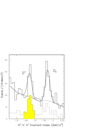
FIG. 2.: Mass spectrum of candidate $K^{+}\pi^{-}\pi^{+}$ events with selection criteria optimized for the branching fraction measurement. The total background, including the contributions shown in Figure 1, is represented by the solid line outside the peaks and the dashed line under the peaks. The dotted histogram shows the mass distribution with tighter selection criteria. The events in the shaded area were used for the Dalitz plot analysis.

The $K^{-}\pi^{+}\pi^{+}$ mass distribution for the sample of CF $D^{+}\to K^{-}\pi^{+}\pi^{+}$ events, selected with the same criteria as the DCS signal and used as the normalization signal, is shown in Figure 3. The spectrum was fit to the sum of a linear background and a Gaussian signal whose parameters were allowed to vary, yielding the values quoted above. The number of $D^{+}\to K^{-}\pi^{+}\pi^{+}$ signal events was found to be $7688\pm 90$.

Using Monte Carlo simulations with resonant and nonresonant decay modes, we found that the product of acceptance and efficiency was the same for the CF and DCS samples within the $\pm 2\%$ statistical errors in the simulations. The ratio of branching fractions for the DCS $D^{+}\to K^{+}\pi^{-}\pi^{+}$ and CF $D^{+}\to K^{-}\pi^{+}\pi^{+}$ decay modes is, thus, given by the ratio of the measured numbers of DCS and CF signal events,

$${B(D^{+}\to K^{+}\pi^{-}\pi^{+})\over B(D^{+}\to K^{-}\pi^{+}\pi^{+})}=(7.7\pm 1.7\pm 0.8)\times 10^{-3}.$$ (1)

The first error reported is statistical. The second is the systematic error, which was dominated by uncertainties in the background shape (8.5%), in the estimated number of background events used in the fit (4%), and the systematic error associated with particle identification (3.8%). The total fractional systematic error is 10%.

Using the PDG value [3] for the CF branching fraction, $(9.1\pm 0.6)$%, we find

$$B(D^{+}\to K^{+}\pi^{-}\pi^{+})=(7.0\pm 1.5\pm 0.9)\times 10^{-4},$$ (2)

where the fractional uncertainty in $B(D^{+}\to K^{-}\pi^{+}\pi^{+})$ has been added in quadrature with our systematic uncertainty in the ratio of branching fractions to determine the systematic error for the absolute DCS branching fraction.

The value we have measured for the ratio of DCS to CF branching fractions is (3.0 $\pm$ 0.8)$\times\tan^{4}\theta_{C}$, which agrees well with the simple spectator picture discussed in the introduction. It also agrees well with the recent result from Fermilab E687[4] for ratio (1), $(7.2\pm 2.3\pm 1.7)\times 10^{-3}$.

FIG. 3.: Mass spectrum of candidate $D^{+}\to K^{-}\pi^{+}\pi^{+}$ events with final optimized selection criteria. The curve is a fit to a Gaussian signal and a linear background. The DCS $D^{+}\to K^{+}\pi^{-}\pi^{+}$ signal was normalized to this signal.

To study the DCS amplitudes which lead to the decay $D^{+}\to K^{+}\pi^{-}\pi^{+}$, we have analyzed the Dalitz plot of a smaller but cleaner sample of events. Because so much of the background in the larger sample comes from misidentified charm decay, we used even more stringent particle identification on the odd-charged pion, which reduced the particle identification efficiency from 22% to 17%. We also required that each candidate’s proper decay time be greater than two $D^{0}$ lifetimes to suppress background from $D^{0}$ and $D_{s}$ decays. We also explicitly removed candidates consistent with the mass hypothesis for $D^{+}\to K^{-}\pi^{+}\pi^{+}$. This tighter selection gives a branching ratio consistent with that from the larger sample (equation (1)), for which selection criteria were chosen to maximize the projected sensitivity. The use of this cleaner sample, which contains 42 $\pm$ 9 signal events, reduced the systematic uncertainties from parametrizing backgrounds in the amplitude analysis. The Dalitz plot analysis was restricted to events found within 30 MeV/$c^{2}$ of the $D^{+}$ mass (67 events altogether). These events correspond to the shaded area in the histogram at the bottom of Figure 2. The Dalitz plot of these events is shown in Figure 4.

FIG. 4.: Dalitz plot ($M^{2}(K^{+}\pi^{-})$ vs. $M^{2}(\pi^{+}\pi^{-})$) of events found within 30 MeV/$c^{2}$ of the $D^{+}$ mass. This sample corresponds to the events in the shaded region of the dotted histogram shown in Figure 2.

The Dalitz plot was fit using the unbinned maximum-likelihood method. The $D^{+}\to K^{+}\pi^{-}\pi^{+}$ decay amplitude was represented by a uniform nonresonant component plus relative amplitudes corresponding to the decays $D^{+}\to K^{+}\rho^{0}(770)$ and $D^{+}\to K^{*0}(890)\pi^{+}$,

$${\cal M}=A_{NR}+\sum_{j=1}^{2}a_{j}e^{i\delta_{j}}R_{j}(m_{K\pi}^{2},m_{\pi\pi}^{2}).$$ (3)

Each resonant component $R_{j}$ was parameterized by a relativistic Breit-Wigner function, of constant width, multiplied by a function describing the angular distribution of decay particles. The nonresonant mode $A_{NR}$ was chosen as the reference channel, fixing the scale for the relative fractions and the phase convention $(A_{NR}\equiv 1)$. The fit parameters were, therefore, the relative phases $\delta_{j}$ and the real positive coefficients $a_{j}$ for each resonant amplitude. The signal likelihood was obtained by multiplying the ideal Dalitz plot density by a function describing the geometrical acceptance and the reconstruction and event-selection efficiencies, including the removal of $\phi\rightarrow K^{+}K^{-}$ and $D^{+}\rightarrow K^{-}\pi^{+}\pi^{+}$ events described above.

The background was represented by the sum of a constant term plus a product of two Gaussians in $K^{+}\pi^{-}$ and $\pi^{+}\pi^{-}$ masses accounting for the $D_{s}\to K^{+}K^{-}\pi^{+}$ reflection, which is concentrated in the upper part of the Dalitz plot. The shape of the $D_{s}$ reflection was obtained from Monte Carlo $D_{s}\to K^{+}K^{-}\pi^{+}$ events that passed through the same selection criteria as for the $K^{+}\pi^{-}\pi^{+}$ sample. We estimate 5 $\pm$ 3 $D_{s}$ decays in the sample shown in Figure 4.

The fit results are shown in Table 1. The decay fractions were computed by integrating the squared amplitude of each mode over the phase space, and then dividing it by the integral of the square of the sum of all amplitudes. As shown in Table 1, the contributions of the three components are comparable. The two resonant modes are approximately in phase with each other and roughly $90^{\circ}$ out of phase with the nonresonant part.

Because of the $D_{s}$ contribution to the cluster of events at the top of the Dalitz plot, the fractions corresponding to the $K^{+}\rho^{0}(770)$ and nonresonant modes are anticorrelated with the estimated number of $D_{s}\to K^{+}K^{-}\pi^{+}$ background events. Changing the estimated $D_{s}$ background to 8 events causes the $K^{+}\rho^{0}(770)$ fraction to decrease by about 0.5 $\sigma$, where $\sigma$ is the statistical uncertainty from the fit, and the nonresonant fraction to increase by the same amount. If, instead, the expected $D_{s}$ background were 2 events, the $K^{+}\rho^{0}(770)$ fraction would increase and nonresonant fraction decrease by 0.5 $\sigma$. These uncertainties dominate the systematic error.

We also attempted to include a $D^{+}\to K^{*}(1430)\pi^{+}$ amplitude in the fit, but this broad ($\Gamma=$ 287 MeV) spin zero resonance could not be distinguished from the nonresonant amplitude.

TABLE I.: Results from the $D^{+}\to K^{+}\pi^{-}\pi^{+}$ Dalitz plot fit. There is an anticorrelated systematic error of $\pm$ 0.07 on the fractions of the nonresonant and $K^{+}\rho^{0}(770)$ modes, due to uncertainty in the estimated number of $D_{s}\to K^{+}K^{-}\pi^{+}$ background events. This uncertainty in $D_{s}$ background has negligible effect on the phases.

mode	phase (radians)	fraction
nonresonant	0 (fixed)	$0.36\pm 0.14\pm 0.07$
$K^{*0}(890)\pi^{+}$	$1.8\pm 0.5$	$0.35\pm 0.14\pm 0.01$
$K^{+}\rho^{0}(770)$	$2.0\pm 0.4$	$0.37\pm 0.14\pm 0.07$

The fit results are also shown in Figure 5 as Monte Carlo density plots. On the left is the generated signal probability distribution function (pdf); on the right is the signal plus background pdf, now multiplied by efficiency and acceptance functions. Due to the more stringent particle-identification criterion adopted for the odd-charged pion candidate, the overall efficiency was reduced at low values of the squared masses. This can be seen clearly by comparing plots a) and b) in Figure 5.

A Monte Carlo technique was used both to test the fitting procedure and to assess the goodness-of-fit. A large number of $K^{+}\pi^{-}\pi^{+}$ samples was generated according to the overall probability distribution function, using as input parameters the phases and coefficients given by the fit to the real data. Each of these Monte Carlo samples was then fitted, and the distributions of the resulting fit parameters were plotted. The average values of all fit parameters were the same as their input values, and the rms spread in each fit parameter distribution was close to the error on this parameter given by the fit of real data. The fraction of Monte Carlo samples for which the value of $-2\ln{({\cal L}_{max})}$ exceeds that of real data, where ${\cal L}_{max}$ is the maximum value of the sample likelihood, estimates the confidence level of our fit to be 52%.

FIG. 5.: Monte  Carlo  simulations  of  the  $D^{+}\to K^{+}\pi^{-}\pi^{+}$  Dalitz  plot for (a) generated signal and (b) accepted signal plus background. Both use the signal parameters of the fit reported in Table I. Plot (b) also includes the background measured for the data of Figure 4. In these plots, the linear dimension of the boxes is proportional to the number of events.

In spite of the large errors on the fractions, the pattern shown in the DCS $D^{+}\to K^{+}\pi^{-}\pi^{+}$ decay appears to differ qualitatively from the corresponding CF decay, in which the nonresonant component corresponds to about 95% of the branching fraction [3].

In summary, Fermilab experiment E791 has measured the ratio of branching fractions for the doubly Cabibbo-suppressed $D^{+}\to K^{+}\pi^{-}\pi^{+}$ and the Cabibbo-favored $D^{+}\to K^{-}\pi^{+}\pi^{+}$ decay modes, $B(D^{+}\to K^{+}\pi^{-}\pi^{+})$ / $B(D^{+}\to K^{-}\pi^{+}\pi^{+})=(7.7\pm 1.7\pm 0.8)\times 10^{-3}$, corresponding to $(3.0\pm 0.8)\,\tan^{4}{\theta_{C}}$. A Dalitz plot analysis indicates that the DCS signal is composed of approximately equal amounts of $D^{+}\to K^{+}\rho^{0}(770)$, $D^{+}\to K^{*0}(890)\pi^{+}$ and nonresonant modes. Using the measured fractions from Table 1 and the $D^{+}\rightarrow K^{+}\pi^{-}\pi^{+}$ branching fraction from equation (2), we obtain $B(D^{+}\rightarrow K^{*0}(890)\pi^{+})=(2.5\pm 1.2)\times 10^{-4}$, $B(D^{+}\rightarrow K^{+}\rho^{0}(770))=(2.6\pm 1.3)\times 10^{-4}$, and $B(D^{+}\rightarrow{\rm{nonresonant~{}}}K^{+}\pi^{-}\pi^{+})=(2.5\pm 1.3)\times 10^{-4}$; statistical and systematic errors have been added in quadrature.

We gratefully acknowledge the assistance of the staffs of Fermilab and of all the participating institutions. This research was supported by the Brazilian Conselho Nacional de Desenvolvimento Científico e Tecnológico, CONACyT (Mexico), the Israeli Academy of Sciences and Humanities, the U.S. Department of Energy, the U.S.-Israel Binational Science Foundation, and the U.S. National Science Foundation. Fermilab is operated by the Universities Research Association, Inc., under contract with the United States Department of Energy.

REFERENCES

- [1] J. A. Appel, Ann. Rev. Nucl. Part. Sci. 42 (1992) 367, and references therein; D. J. Summers et al., Proceedings of the XXVIIth Rencontre de Moriond, Electroweak Interactions and Unified Theories, Les Arcs, France (15 - 22 March 1992) 417; S. Amato et al., Nucl. Instr. Meth. A324 (1993) 535.
- [2] D. Bartlett et al., Nucl. Instr. Meth. A260 (1987) 55.
- [3] Particle Data Group, L. Montanet et al., Phys. Rev. D54 (1996) 1.
- [4] P. L. Frabetti et al., Phys. Lett. B359 (1995) 403.