A New Measurement of $B\to D^{*}\pi$ Branching Fractions

Abstract

The decays $\Upsilon(4S)\!\to\!B\overline{B}$, followed by $B\!\to\!D^{*}\pi$ and $D^{*}\!\to\!D\pi$, permit reconstruction of all kinematic quantities that describe the sequence without reconstruction of the $D$, with reasonably low backgrounds. Using an integrated $e^{+}e^{-}$ luminosity of 3.1 ${\rm fb}^{-1}$ accumulated at the $\Upsilon$(4S) by the CLEO-II detector, we report measurements of ${\cal B}({\overline{B}^{0}\!\to\!{D^{*+}}\,{\pi^{-}}})={(2.81\pm 0.11\pm 0.21\pm 0.05)\times 10^{-3}}$ and ${\cal B}({{B}^{-}\!\to\!{D^{*0}}\,{\pi^{-}}})={(4.34\pm 0.33\pm 0.34\pm 0.18)\times 10^{-3}}$.

G. Brandenburg,¹ R. A. Briere,¹ Y. S. Gao,¹ D. Y.-J. Kim,¹ R. Wilson,¹ H. Yamamoto,¹ T. E. Browder,² F. Li,² Y. Li,² J. L. Rodriguez,² T. Bergfeld,³ B. I. Eisenstein,³ J. Ernst,³ G. E. Gladding,³ G. D. Gollin,³ R. M. Hans,³ E. Johnson,³ I. Karliner,³ M. A. Marsh,³ M. Palmer,³ M. Selen,³ J. J. Thaler,³ K. W. Edwards,⁴ A. Bellerive,⁵ R. Janicek,⁵ D. B. MacFarlane,⁵ K. W. McLean,⁵ P. M. Patel,⁵ A. J. Sadoff,⁶ R. Ammar,⁷ P. Baringer,⁷ A. Bean,⁷ D. Besson,⁷ D. Coppage,⁷ C. Darling,⁷ R. Davis,⁷ N. Hancock,⁷ S. Kotov,⁷ I. Kravchenko,⁷ N. Kwak,⁷ S. Anderson,⁸ Y. Kubota,⁸ M. Lattery,⁸ S. J. Lee,⁸ J. J. O’Neill,⁸ S. Patton,⁸ R. Poling,⁸ T. Riehle,⁸ V. Savinov,⁸ A. Smith,⁸ M. S. Alam,⁹ S. B. Athar,⁹ Z. Ling,⁹ A. H. Mahmood,⁹ H. Severini,⁹ S. Timm,⁹ F. Wappler,⁹ A. Anastassov,¹⁰ S. Blinov,^10, J. E. Duboscq,¹⁰ K. D. Fisher,¹⁰ D. Fujino,^10, R. Fulton,¹⁰ K. K. Gan,¹⁰ T. Hart,¹⁰ K. Honscheid,¹⁰ H. Kagan,¹⁰ R. Kass,¹⁰ J. Lee,¹⁰ M. B. Spencer,¹⁰ M. Sung,¹⁰ A. Undrus,^10,∗ R. Wanke,¹⁰ A. Wolf,¹⁰ M. M. Zoeller,¹⁰ B. Nemati,¹¹ S. J. Richichi,¹¹ W. R. Ross,¹¹ P. Skubic,¹¹ M. Wood,¹¹ M. Bishai,¹² J. Fast,¹² E. Gerndt,¹² J. W. Hinson,¹² N. Menon,¹² D. H. Miller,¹² E. I. Shibata,¹² I. P. J. Shipsey,¹² M. Yurko,¹² L. Gibbons,¹³ S. D. Johnson,¹³ Y. Kwon,¹³ S. Roberts,¹³ E. H. Thorndike,¹³ C. P. Jessop,¹⁴ K. Lingel,¹⁴ H. Marsiske,¹⁴ M. L. Perl,¹⁴ S. F. Schaffner,¹⁴ D. Ugolini,¹⁴ R. Wang,¹⁴ X. Zhou,¹⁴ T. E. Coan,¹⁵ V. Fadeyev,¹⁵ I. Korolkov,¹⁵ Y. Maravin,¹⁵ I. Narsky,¹⁵ V. Shelkov,¹⁵ J. Staeck,¹⁵ R. Stroynowski,¹⁵ I. Volobouev,¹⁵ J. Ye,¹⁵ M. Artuso,¹⁶ A. Efimov,¹⁶ F. Frasconi,¹⁶ M. Gao,¹⁶ M. Goldberg,¹⁶ D. He,¹⁶ S. Kopp,¹⁶ G. C. Moneti,¹⁶ R. Mountain,¹⁶ S. Schuh,¹⁶ T. Skwarnicki,¹⁶ S. Stone,¹⁶ G. Viehhauser,¹⁶ X. Xing,¹⁶ J. Bartelt,¹⁷ S. E. Csorna,¹⁷ V. Jain,¹⁷ S. Marka,¹⁷ A. Freyberger,¹⁸ R. Godang,¹⁸ K. Kinoshita,¹⁸ I. C. Lai,¹⁸ P. Pomianowski,¹⁸ S. Schrenk,¹⁸ G. Bonvicini,¹⁹ D. Cinabro,¹⁹ R. Greene,¹⁹ L. P. Perera,¹⁹ G. J. Zhou,¹⁹ B. Barish,²⁰ M. Chadha,²⁰ S. Chan,²⁰ G. Eigen,²⁰ J. S. Miller,²⁰ C. O’Grady,²⁰ M. Schmidtler,²⁰ J. Urheim,²⁰ A. J. Weinstein,²⁰ F. Würthwein,²⁰ D. M. Asner,²¹ D. W. Bliss,²¹ W. S. Brower,²¹ G. Masek,²¹ H. P. Paar,²¹ V. Sharma,²¹ J. Gronberg,²² T. S. Hill,²² R. Kutschke,²² D. J. Lange,²² S. Menary,²² R. J. Morrison,²² H. N. Nelson,²² T. K. Nelson,²² C. Qiao,²² J. D. Richman,²² D. Roberts,²² A. Ryd,²² M. S. Witherell,²² R. Balest,²³ B. H. Behrens,²³ K. Cho,²³ W. T. Ford,²³ H. Park,²³ P. Rankin,²³ J. Roy,²³ J. G. Smith,²³ J. P. Alexander,²⁴ C. Bebek,²⁴ B. E. Berger,²⁴ K. Berkelman,²⁴ K. Bloom,²⁴ D. G. Cassel,²⁴ H. A. Cho,²⁴ D. M. Coffman,²⁴ D. S. Crowcroft,²⁴ M. Dickson,²⁴ P. S. Drell,²⁴ K. M. Ecklund,²⁴ R. Ehrlich,²⁴ R. Elia,²⁴ A. D. Foland,²⁴ P. Gaidarev,²⁴ B. Gittelman,²⁴ S. W. Gray,²⁴ D. L. Hartill,²⁴ B. K. Heltsley,²⁴ P. I. Hopman,²⁴ J. Kandaswamy,²⁴ N. Katayama,²⁴ P. C. Kim,²⁴ D. L. Kreinick,²⁴ T. Lee,²⁴ Y. Liu,²⁴ G. S. Ludwig,²⁴ J. Masui,²⁴ J. Mevissen,²⁴ N. B. Mistry,²⁴ C. R. Ng,²⁴ E. Nordberg,²⁴ M. Ogg,^24, J. R. Patterson,²⁴ D. Peterson,²⁴ D. Riley,²⁴ A. Soffer,²⁴ C. Ward,²⁴ M. Athanas,²⁵ P. Avery,²⁵ C. D. Jones,²⁵ M. Lohner,²⁵ C. Prescott,²⁵ J. Yelton,²⁵ and J. Zheng²⁵

The study of $B$ decays to exclusively hadronic final states has been limited because samples in available data are small. In this paper we employ a technique, a “partial reconstruction,” that can increase the acceptance of the sequence $\Upsilon$(4S)$\to\!B\overline{B}$, $B\!\to\!D^{*}\pi$, $D^{*}\!\to\!D\pi$, by one order of magnitude with respect to the more usual technique, “full reconstruction,” where all particles in the final state are reconstructed. For example, in a recent analysis [1] using the latter technique, $248$ out of $\sim\!8700$ possible $\overline{B}^{0}\!\to\!{D^{*+}}\,{\pi^{-}}$ decays were reconstructed; in this letter, we report the reconstruction of $\sim\!2600$ $\overline{B}^{0}\!\to\!{D^{*+}}\,{\pi^{-}}$ from the same set of data. We report on the measurement of two of the ${B}\!\to\!{D^{*}}\,{\pi}$ branching fractions with partial reconstruction, and we probe the factorization hypothesis. The partial reconstruction might enable an interesting sensitivity to a small $CP$ asymmetry in $\overline{B}^{0}\!\to\!{D^{*+}}\,{\pi^{-}}$ decays [2].

Both the CLEO [1, 3] and ARGUS [4] collaborations reported measurements of ${B}\!\to\!{D^{*}}\,{\pi}$ based on the full reconstruction technique. In the analysis of data presented in this letter, all kinematic quantities that describe the decay chain $B\rightarrow D^{*}\pi_{f}$, $D^{*}\rightarrow D\pi_{s}$ are reconstructed from measurements of the three-momenta of the two pions, one fast ($\pi_{f}$) and one slow ($\pi_{s}$), $\vec{p}_{f}$ and $\vec{p}_{s}$; the $D$ from $D^{*}$ decay is undetected, which yields an order of magnitude increase in acceptance over full reconstruction, and removes systematic uncertainty introduced by $D$ branching fractions.

The basic idea was described in [5]: a $B$ from $\Upsilon(4S)$ decay is nearly at rest and the energy release in the $D^{*}\rightarrow D\pi$ decay is small, so the decay products , $\pi_{s}$ and $\pi_{f}$, are nearly back to back. The smearing introduced in [5] by neglect of the detailed kinematics of the decay sequence is much larger than the smearing caused by errors in either the measurement of the pion momenta, or by the error in knowledge of the magnitude of the initial $B$ momentum. Complete evaluation of the detailed kinematics leads to a significant improvement in the description of the shape of the signal, the shape of the background, and rejection of the background.

To fully describe the kinematics of the decay, twenty parameters are required: four for each four-vector of the five particles: $B$, $D^{*}$, $\pi_{f}$, $D$, and $\pi_{s}$. Energy-momentum conservation can be applied twice, in the $B\rightarrow D^{*}\pi_{f}$ and $D^{*}\rightarrow D\pi_{s}$ decays, yielding eight equations; the masses of the five particles can be assumed; and the center-of-mass energy of the $e^{+}e^{-}$ collisions can be used to obtain the magnitude of the three-momentum of the initial $B$. The six free parameters that remain describe the kinematics of the decay sequence. These can be thought of as six angles: two that describe the $B$ direction, two angles ($\theta^{*}_{f}$,$\phi^{*}_{f}$) that describe the direction of the $\pi_{f}$ in the $B$ rest frame, and two angles ($\theta^{*}_{s}$,$\phi^{*}_{s}$) that describe the direction of the $\pi_{s}$ in the $D^{*}$ rest frame. We evaluate those six angles from the measurement of the three components of the $\pi_{f}$ momentum and the three components of the $\pi_{s}$ momentum.

The angles that provide effective discrimination between signal and background are $\theta^{*}_{f}$ and $\theta^{*}_{s}$, for which the explicit expressions are:

$$\cos\theta^{*}_{f} = \frac{-\beta_{B}(E^{*}_{f}-E^{*}_{D^{*}})}{2P^{*}_{f}}+\frac{{\left|\vec{p}_{f}\right|}^{2}-{\left|P_{D^{*}}\right|}^{2}}{2\gamma_{B}^{2}\beta_{B}M_{B}P^{*}_{f}}{\rm\ \ \;\;and}$$ (1)

$$\cos\theta^{*}_{s} = \frac{-\beta_{D^{*}}(E^{*}_{s}-E^{*}_{D})}{2P^{*}_{s}}+\frac{{\left|\vec{p}_{s}\right|}^{2}-{\left|P_{D}\right|}^{2}}{2\gamma_{D^{*}}^{2}\beta_{D^{*}}M_{D^{*}}P^{*}_{s}},$$ (2)

where $E^{*}_{f}$, $E^{*}_{D^{*}}$ and $P^{*}_{f}$ are the energy and momentum of the $\pi_{f}$ and $D^{*}$ in the $B$ center of mass; $E^{*}_{s}$, $E^{*}_{D}$ and $P^{*}_{s}$ are the energy and momentum of the $\pi_{s}$ and $D$ in the $D^{*}$ center of mass; $\gamma_{B(D^{*})}$, $\beta_{B(D^{*})}$ and $M_{B(D^{*})}$ are the Lorentz factor, the velocity and the mass of the $B(D^{*})$ in the lab frame. The magnitude of the $D^{*}$ and $D$ momenta in the lab frame, $\left|P_{D^{*}}\right|$ and $\left|P_{D}\right|$, are determined by applying energy-momentum conservation in the decay chain. For signal, the magnitudes of these cosines will tend to fall into the ‘physical’ region; less than one. The signal distribution will be uniform in $\cos\theta^{*}_{f}$ (because the $B$ has spin 0), and as $\cos^{2}\theta^{*}_{s}$ (because the $D^{*}$ has helicity 0), before consideration of detector acceptance, efficiency, and resolution. Detector resolution sometimes pushes signal events into the ‘non-physical’ region, where the magnitude of one or both of the cosines exceeds unity. Backgrounds usually fall into the non-physical region. The variables $\cos\theta^{*}_{f}$ and $\cos\theta^{*}_{s}$ tend to depend linearly on $|\vec{p}_{f}|$ and $|\vec{p}_{s}|$ once the dependence of $\left|P_{D^{*}}\right|$ and $\left|P_{D}\right|$ on these variables is included.

The angle between the plane of the $B\rightarrow D^{*}\pi_{f}$ decay and the plane of the $D^{*}\rightarrow D\pi_{s}$ decay, $\phi=\phi^{*}_{f}-\phi^{*}_{s}$, is reconstructed in the following manner. In the lab frame, the $D^{*}$ direction must lie on a small cone of angle $\alpha_{f}$ around the direction opposite to the $\pi_{f}$. Simultaneously, the $D^{*}$ must also lie on a second small cone of angle $\alpha_{s}$ around the direction of the $\pi_{s}$. The expressions for these angles are:

$$\cos\alpha_{f}=\frac{M_{B}^{2}-M_{D^{*}}^{2}-M_{\pi}^{2}}{2\left|P_{D^{*}}\right|\left|\vec{p}_{f}\right|}-\frac{1}{\beta_{D^{*}}\beta_{f}}{\rm\ \ \;\;and\;\;}\cos\alpha_{s}=-\frac{M_{D^{*}}^{2}+M_{\pi}^{2}-M_{D}^{2}}{2\left|P_{D^{*}}\right|\left|\vec{p}_{s}\right|}+\frac{1}{\beta_{D^{*}}\beta_{s}},$$ (3)

where the momenta and velocities are measured in the lab frame. The decay kinematics limit $\alpha_{f}\leq 0.14$ and $\alpha_{s}\leq 0.28$. Intersection of these two cones determines the $D^{*}$ directions, of which in practice there are two: a so-called quadratic ambiguity. For both $D^{*}$ directions:

$$\cos\phi=\frac{\cos\delta-\cos\alpha_{f}\cos\alpha_{s}}{\sin\alpha_{f}\sin\alpha_{s}},$$ (4)

where $\delta$ is the angle between $\vec{p}_{s}$ and the direction opposite to $\vec{p}_{f}$. For most signal events $|\cos\phi|<1$, or ‘physical’. Signal events with imperfect measurement of the pion momenta, as well as non-signal events, can result in $|\cos\phi|>1$, in most cases because $\delta>\alpha_{f}+\alpha_{s}$.

The data used in this analysis were selected from hadronic events produced in $e^{+}e^{-}$ annihilations at the Cornell Electron Storage Ring (CESR). The data sample consists of 3.1 ${\rm fb}^{-1}$ collected with the CLEO-II detector [6] at the $\Upsilon{(4S)}$ resonance (referred to as ‘on-resonance’) and 1.6 ${\rm fb}^{-1}$ at a center-of-mass energy just below the threshold for production of ${B}\overline{B}$ pairs (referred to as ‘off-resonance’). The on-resonance data correspond to $(3.27\pm 0.06)\times 10^{6}$ ${B}\overline{B}$ pairs. The off-resonance data are used to model the background from non-${B}\overline{B}$ decays.

Charged pions that are consistent with production at the $e^{+}e^{-}$ annihilation position and that penetrate all layers of the CLEO II tracking system are identified by means of time-of-flight, specific ionization, and shower development in the CsI calorimeter and surrounding muon identifier. Neutral pions are reconstructed primarily from information in the CsI calorimeter [6].

Events with two pions are classified according to the net charge, which is $0$ or $\pm 1$ for signal. The fast pion is charged, but the slow pion can be either charged ($\pi_{f}^{-}\pi_{s}^{+}$) or neutral ($\pi_{f}^{-}\pi_{s}^{0}$). Only $D^{*\pm}$ decays yield slow charged pions, but slow neutral pions are produced from both $D^{*0}$ and $D^{*\pm}$ decays, and so the $\pi_{f}^{-}\pi_{s}^{0}$ sample will contain contributions from both $\overline{B}^{0}\!\to\!{D^{*+}}\,{\pi^{-}}$ and ${B}^{-}\!\to\!{D^{*0}}\,{\pi^{-}}$. We further require that events satisfy the “$D^{*}$ cone overlap requirement”: $\left|\cos\delta-\cos\alpha_{f}\cos\alpha_{s}\right|<\sin\alpha_{f}\sin\alpha_{s}+0.02$, which allows for detector resolution.

Some events satisfy all requirements two or more times, usually through combinations of one fast pion with several distinct slow pions. In signal Monte Carlo studies, 5% (24%) of $\pi_{f}^{-}\pi_{s}^{+}$ ($\pi_{f}^{-}\pi_{s}^{0}$) events have more than one possible slow charged (neutral) pion. In $\pi_{f}^{-}\pi_{s}^{0}$ events, we select the neutral pion whose mass is closest to the nominal $\pi^{0}$ mass and in $\pi_{f}^{-}\pi_{s}^{+}$ events the two pion candidate with the smallest value of $\left|\cos\delta-\cos\alpha_{f}\cos\alpha_{s}\right|$ is selected.

The dominant sources of background are non-${B}\overline{B}$ events. The distribution of decay products in these events tends to be jet-like, while in ${B}\overline{B}$ events the decay products tend to be distributed uniformly in angle. To suppress non-${B}\overline{B}$ events, each candidate event must satisfy $R_{2}<0.275$, where $R_{2}$ is the ratio of the second Fox-Wolfram moment to the zeroth moment [7]. We also reject events where the momentum of any charged track exceeds the maximum possible from a $B$ decay, 2.45 GeV/c.

To extract the branching fractions we perform a two-dimensional fit in $\cos{\theta^{*}_{f}}$ and $\cos{\theta^{*}_{s}}$, where the fit region is $|{\cos{\theta^{*}_{f}}}|<1.65$ and $-1.6<{\cos{\theta^{*}_{s}}}<5.0$. The $\pi_{f}^{-}\pi_{s}^{+}$ and $\pi_{f}^{-}\pi_{s}^{0}$ data samples are fit simultaneously using the MINUIT [8] program. The fitting function combines contributions from the ${B}\!\to\!{D^{*}}\,{\pi}$ signal, other $B$ decays, and a fixed amount of non-${B}\overline{B}$ background as described below.

The non-${B}\overline{B}$ background shape and rate is determined from a sample of off-resonance data, that has been scaled for the relative luminosities and cross-sections between the on-resonance and off-resonance data samples. The $\cos{\theta^{*}_{f}}$ and $\cos{\theta^{*}_{s}}$ distributions in non-${B}\overline{B}$ events are primarily determined by the ${\pi}_{f}$ and ${\pi}_{s}$ momentum spectra in those events. Additionally, the shape is affected by the $D^{*}$ cone overlap requirement, which admits the most events when $\alpha_{s}$ is largest, which occurs roughly when $\cos{\theta^{*}_{s}}$ $\approx 0$. The shape of the background is thus roughly $\propto\sin^{2}\theta^{*}_{s}$, which is the complement of the signal, $\propto\cos^{2}\theta^{*}_{s}$.

A large sample of simulated ${B}\overline{B}$ events shows that this background is dominated by modes that are able to produce a fast pion candidate, such as $B\rightarrow D^{(\pm,0)}X$, where the $X$ system is predominantly $\pi$, $\rho$ or $\mu\nu_{\mu}$, and the $D^{(\pm,0)}$ can be in an excited state. The background distribution in $\cos\theta_{f}^{*}$ is determined by the kinematics of the fast pion from the $B$ decay. Slow pions are plentiful in these ${{B}\overline{B}}$ background samples. When fast and slow pion candidates come from different $B$’s, the resulting distribution in $\cos\theta_{s}^{*}$ resembles the non-${B}\overline{B}$ distribution. When both candidates come from the same $B$ decay, the distribution in $\theta_{s}^{*}$ and $\theta_{f}^{*}$ is distinctive, but unlike that of the signal: the branching ratios of modes that enter the final sample in this manner are allowed to float in the final fit, either constrained by a Gaussian to the central value and error in [9], or left unconstrained, if no measurement is available. The branching fractions used in the $\pi_{f}^{-}\pi_{s}^{+}$ and the $\pi_{f}^{-}\pi_{s}^{0}$ samples are constrained to be equal.

One $B$ decay background mode is handled differently. The Cabibbo-suppressed mode ${B}\!\to\!{D^{*}}\,K$ is essentially indistinguishable from ${B}\!\to\!{D^{*}}\,{\pi}$ in the partial reconstruction. We assume that the ratio of branching fractions, ${\cal B}({{B}\!\to\!{D^{*}}\,K})/{\cal B}({{B}\!\to\!{D^{*}}\,{\pi}})$, is given by the ratio of the decay constants for kaons and pions, $f_{K}/f_{\pi}$, the ratio of the CKM matrix elements, $V_{us}/V_{ud}$, and the ratio of form factors. The product of these ratios is determined to be ($7.69\pm 0.08$)% [10, 11]. The assumed ${B}\!\to\!{D^{*}}\,K$ rate is subtracted, with adjustment for acceptance.

The projections of the data and the fitting function in $\cos{\theta^{*}_{f}}$ and $\cos{\theta^{*}_{s}}$ are shown in Fig. 1 for the $\pi_{f}^{-}\pi_{s}^{+}$ fit and in Fig. 2 for the $\pi_{f}^{-}\pi_{s}^{0}$ fit. The sidebands outside the signal region tend to determine the background normalization, and are fitted well by the background functions. The sharp turn-on of signal at $\pm 1$ can be seen while the background distribution in $\cos{\theta^{*}_{s}}$ shows the expected peaking in the signal region due to the $D^{*}$ cone overlap requirement. The confidence level for the $\pi_{f}^{-}\pi_{s}^{+}$($\pi_{f}^{-}\pi_{s}^{0}$) fit alone is 29%(2%). No structure is observed in the residuals of the fit and confidence level for the combined fit is 3%. The fitted number of signal events is given in Tab. I along with the product of acceptance and efficiency and the relevant $D^{*}$ branching fraction. The background subtracted plots for the $\pi_{f}^{-}\pi_{s}^{+}$ and $\pi_{f}^{-}\pi_{s}^{0}$ fits for the $\cos{\theta^{*}_{s}}$ projection are shown in Fig. 3. The peaks are asymmetric because the acceptance functions for charged and neutral slow pions have momentum dependences.

The systematic uncertainty was determined to be 7.5% for $\overline{B}^{0}\!\to\!{D^{*+}}\,{\pi^{-}}$ and 8.3% for ${B}^{-}\!\to\!{D^{*0}}\,{\pi^{-}}$. The error is dominated by uncertainties in the slow pion reconstruction efficiency, $B$ decay background shape and simulation of the $R_{2}$ requirement. Additional errors come from the uncertainty in the number of ${B}\overline{B}$ pairs produced, signal shape smearing, Monte Carlo statistics and the simulation of $\cos\delta$.

To convert from fitted yields to branching fractions we use the value of $(3.27\pm 0.06)\times 10^{6}$ ${B}\overline{B}$ pairs produced and assume that the ratio of $B^{+}B^{-}$ to $B^{0}\overline{B}^{0}$ production ($f_{+-}/f_{00}$) is one. This is in agreement with the current CLEO measurement of $f_{+-}\tau_{B^{\pm}}/f_{00}\tau_{B^{0}}=1.15\pm 0.17\pm 0.06$ [12] and the value [9] for the ratio of lifetimes $\tau_{B^{\pm}}/\tau_{B^{0}}=1.03\pm 0.06$. We find:

$${\cal B}(\overline{B}^{0}\to\ D^{*+}\pi^{-})={(2.81\pm 0.11\pm 0.21\pm 0.05)\times 10^{-3}}$$ (5)

$${\cal B}(B^{-}\to\ D^{*0}\pi^{-})={(4.34\pm 0.33\pm 0.34\pm 0.18)\times 10^{-3}}$$ (6)

where the first error is statistical, the second is systematic, and the third comes from the uncertainty in the ${D^{*}}\!\to\!{D}{\pi}$ branching fractions.

To compare with the factorization hypothesis [13], we take the ratio of charged to neutral branching fractions, in which the systematic uncertainties due to the number of $B\overline{B}$ events, the $R_{2}$ requirement, and the fast pion reconstruction cancel. The ratio is measured to be $r=1.55\pm 0.14\pm 0.15$.

An implementation of the factorization hypothesis[14] predicts that $r$ is equal to $(1+1.29\ a_{2}/a_{1})^{2}$. The coefficient $a_{1}\!\approx\!1$ describes the ‘external spectator amplitude,’ where the $W$ hadronizes to a single pion, and $a_{2}$ describes the internal, color-suppressed amplitudes, and is expected to be rather smaller than 1. The measurement of $r$ yields $a_{2}/a_{1}$ of $0.19\pm 0.04\pm 0.05$. Another ratio, ${\cal B}(\overline{B}^{0}\!\to\!D^{*0}\pi^{0})/{\cal B}(\overline{B}^{0}\!\to\!D^{*+}\pi^{-})$ is given by $0.84\times(a_{2}/a_{1})^{2}$ using the same model. From the results quoted above, the factorization hypothesis predicts, in the absence of final state interactions, ${\cal B}(\overline{B}^{0}\!\to\!D^{*0}\pi^{0})=8.5\times 10^{-5}$, about five times smaller than the current [15] experimental limit.

We searched for the suppressed modes which produce a fast neutral pion. In $\pi_{f}^{0}\pi_{s}^{+}$ events no signal was observed. The confidence level of the fit was 73% indicating good agreement between the background shape and the data. We limit the doubly CKM-suppressed mode to ${\cal B}(B^{-}\!\to\!D^{*-}\pi^{0})<1.7\times 10^{-4}$ at 90% confidence level. For internal color-suppressed modes the superior background rejection of the full reconstruction technique [15] leads to better sensitivity, except in the case of $\overline{B}^{0}\!\to\!D^{*0}\eta^{\prime}$. We set a limit of ${\cal B}(\overline{B}^{0}\!\to\!D^{*0}\eta^{\prime})<14\times 10^{-4}$ at 90% confidence level. The confidence level of the fit was 10%.

We gratefully acknowledge the effort of the CESR staff in providing us with excellent luminosity and running conditions. This work was supported by the National Science Foundation, the U.S. Department of Energy, the Heisenberg Foundation, the Alexander von Humboldt Stiftung, Research Corporation, the Natural Sciences and Engineering Research Council of Canada, and the A.P. Sloan Foundation.

TABLE I.: The yield of signal events from the fits. The D* branching fractions are not included in the calculation of acceptance times efficiency.

Mode	Yield	Acc. $\times$ Eff.	${\cal B}$($D^{*}\!\to\!D\pi$)
$\overline{B}^{0}\!\to\!D^{*+}\pi^{-};D^{*+}\!\to\!D^{0}\pi^{+}$	$2612\pm 102$	0.42	68.3%
$\overline{B}^{0}\!\to\!D^{*+}\pi^{-};D^{*+}\!\to\!D^{+}\pi^{0}$	$513\pm 21$	0.18	30.6%
$B^{-}\!\to\!D^{*0}\pi^{-};D^{*0}\!\to\!D^{0}\pi^{0}$	$1560\pm 115$	0.18	61.9%

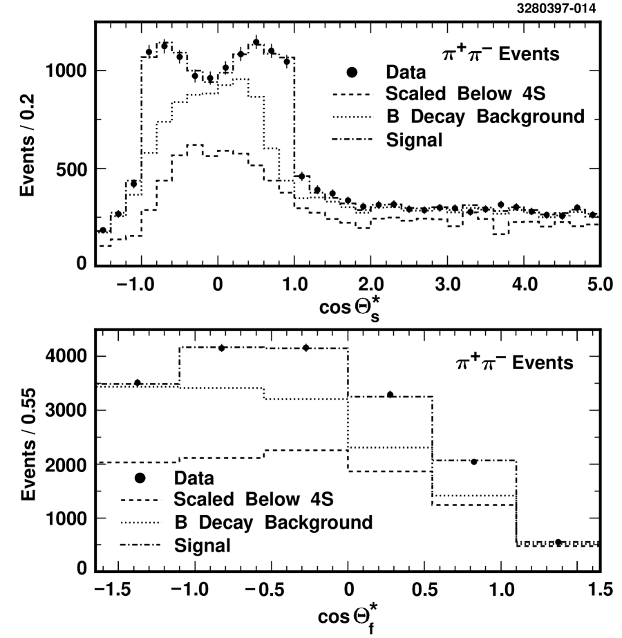
FIG. 1.: The projections of the data histogram in $\cos{\theta^{*}_{f}}$ and $\cos{\theta^{*}_{s}}$ with the fitting function for the $\pi_{f}^{-}\pi_{s}^{+}$ fit.

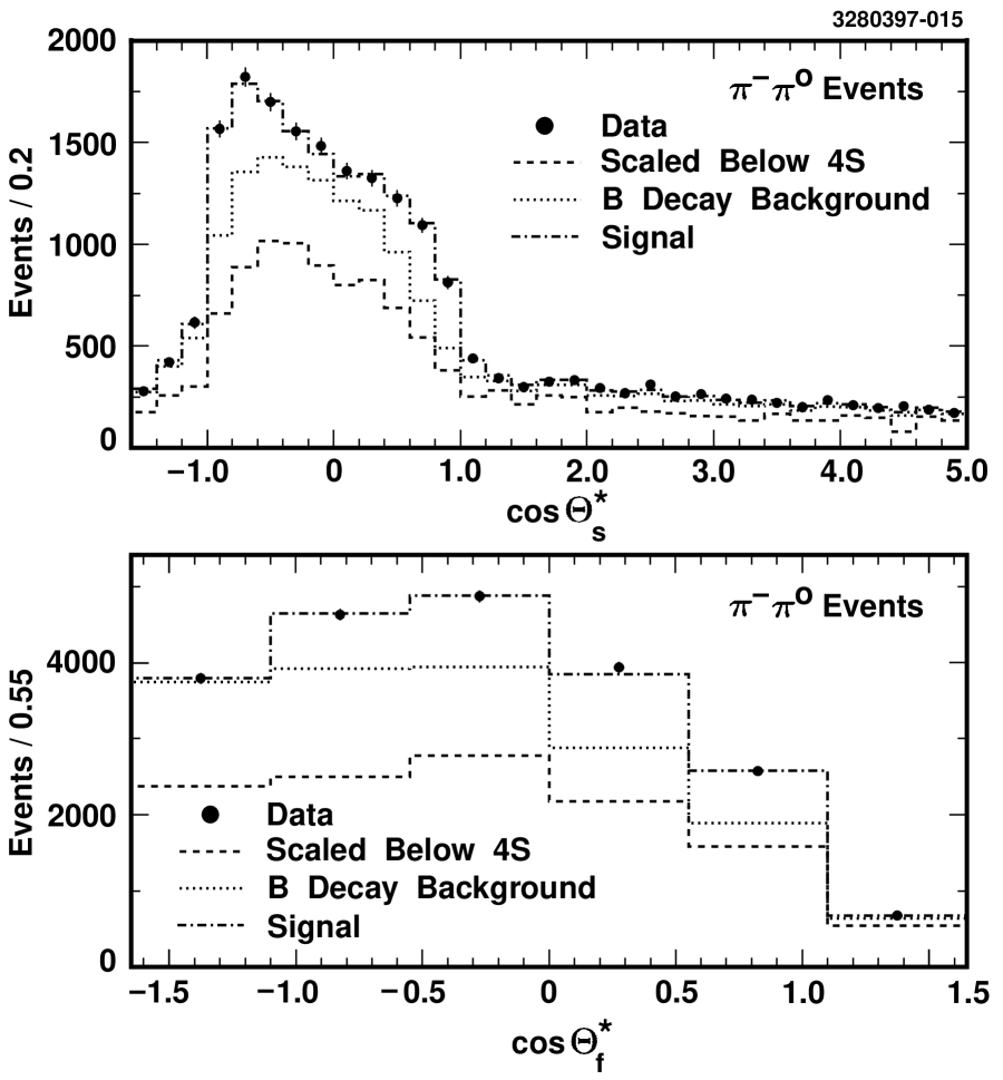
FIG. 2.: The projections of the data histogram in $\cos{\theta^{*}_{f}}$ and $\cos{\theta^{*}_{s}}$ with the fitting function for the $\pi_{f}^{-}\pi_{s}^{0}$ fit.

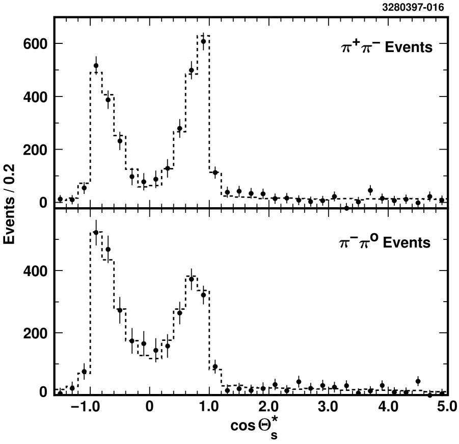
FIG. 3.: The background-subtracted projections of the data histogram in $\cos{\theta^{*}_{s}}$ for the $\pi_{f}^{-}\pi_{s}^{+}$ and $\pi_{f}^{-}\pi_{s}^{0}$ fits. The dashed line is the signal shape.

REFERENCES

- [1] B. Barish et al., contribution to the 1997 European Physical Society meeting, Jerusalem (preprint CLEO CONF 97-01, August 1997) (unpublished).
- [2] R. G. Sachs, Report No. EFI-85-22, Chicago, 1985 (unpublished); R. G. Sachs, The Physics of Time Reversal (The University of Chicago Press, Chicago, IL, 1987), pp. 257-261; I. I. Bigi and A. I. Sanda, Nucl. Phys. B281, 41 (1987); I. Dunietz and R. G. Sachs, Phys. Rev. D37, 3186 (1988).
- [3] CLEO Collab., M. S. Alam et al., Phys. Rev. D50, 43 (1994).
- [4] ARGUS Collab., H. Albrecht et al., Z. Phys. C48, 543 (1990).
- [5] CLEO Collab., R. Giles et al., Phys. Rev. D30, 2279 (1984).
- [6] CLEO Collab., Y. Kubota et al., Nucl. Instr. and Meth. A320, 66 (1992).
- [7] G. C. Fox and S. Wolfram, Phys. Rev. Lett. 41, 1581 (1978).
- [8] I. Brock, A Fitting and Plotting Package Using MINUIT, CLEO/CSN Note 245-B, Revised (1992) (unpublished); F. James, MINUIT, Function Minimization and Error Analysis, CERN Program Library Long Writeup D506, Mar. 1994 (unpublished).
- [9] R. M. Barnett et al., Phys. Rev. D54, 488-506 (1996).
- [10] R. M. Barnett et al., Phys. Rev. D54, 94, 319 (1996).
- [11] M. Neubert and B. Stech, preprint hep-ph/9705292, to appear in: the Second Edition of Heavy Flavours, edited by A. J. Buras and M. Linder (World Scientific, Singapore).
- [12] CLEO Collab., C. S. Jessop et al., Phys. Rev. Lett. 79, 4533 (1997).
- [13] M. Bauer, B. Stech, and M. Wirbel, Z. Phys. C29, 637 (1985).
- [14] M. Neubert, V. Rieckert, B. Stech and Q. P. Xu in Heavy Flavours, edited by A. J. Buras and H. Lindner (World Scientific, Singapore, 1992).
- [15] CLEO Collab., B. Nemati et al., CLNS 97/1503 (submitted to Phys. Rev. D).