SLAC–PUB–7434

MIT-LNS-97-267

March 1997

PRECISE TESTS OF QCD

IN

e⁺e^- ANNIHILATION^∗

P.N. Burrows^∗∗

Stanford Linear Accelerator Center

Stanford University, Stanford, CA94309, USA

burrows@slac.stanford.edu

ABSTRACT

A pedagogical review is given of precise tests of QCD in electron-positron annihilation. Emphasis is placed on measurements that have served to establish QCD as the correct theory of strong interactions, as well as measurements of the coupling parameter $\alpha_{s}$. An outlook is given for future important tests at a high-energy e⁺e^-collider.

Lectures given at the SLAC Summer Institute,

August 19-30, 1996

$\star$ Work supported by Department of Energy contracts DE–FC02–94ER40818 (MIT) and DE–AC03–76SF00515 (SLAC).

$**$ Permanent address: Lab. for Nuclear Science, M.I.T., Cambridge, MA 02139, USA.

1. Introduction - e⁺e^-Colliders

The production of hadronic final-states by a variety of interactions is illustrated in Fig. 1. In electron-positron annihilation hadronic activity is, by construction, limited to the final state, making the study of hadronic events cleaner and simpler relative to lepton-hadron and hadron-hadron collisions, from both the experimental and theoretical points-of-view. On the experimental side there are no remnants of the beam particles to add confusion to the interpretation of hadronic structures, and, apart from initial and final-state photon radiation effects, the hadronic centre-of-mass frame coincides with the laboratory frame. On the theoretical side the absence of hadrons in the incoming beams removes dependence on the limited knowledge of the parton density functions of hadrons, as well as rendering QCD calculations at a given order of perturbation theory easier to perform because there are generally fewer strong-interaction Feynman diagrams to consider. Electron-positron annihilation thus provides an ideal environment for precise tests of QCD.

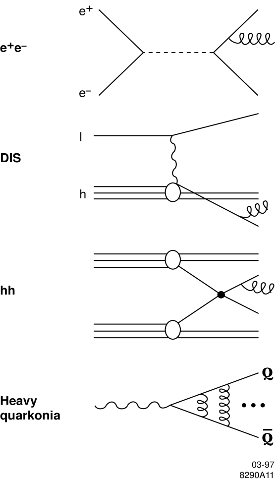
Figure 1: Schematic of the production of hadronic final-states by different interactions: e⁺e^-annihilation, deep inelastic lepton-hadron scattering, hadron-hadron collisions, and production and decay of heavy quarkonia.

A large number of e⁺e^-colliders have been constructed over the past 25 years; these are listed in Table 1. The range of c.m. energies $Q$ extends from a few GeV at the very first colliders up to almost 200 GeV at the CERN LEP-II collider. The first generation of colliders was built on speculation of allowing exciting high-energy physics studies. They did not disappoint, the J/$\Psi$ being discovered at SPEAR, the gluon being observed at PETRA, and a wealth of strong- and electroweak-interaction studies being performed at PETRA, PEP, and TRISTAN, all of which served to establish the validity of the Standard Model. A second generation of colliders has been designed to serve as particle ‘factories’: DA$\Phi$NE in the vicinity of the $\Phi$ resonance, BEPC near the charmonium threshold, DORIS, CESR, PEP-II and KEKB around the bottomonium resonances, SLC and LEP at the $Z^{0}$ resonance, and LEP-II at the W⁺W^- threshold.

	Collider	Location	c.m. energy $Q$ (GeV)
	ADONE	Frascati	1 $-$ 3
	DCI	Orsay	1 $-$ 2.4
$\bullet$	VEPP-2M	Novosibirsk	1 $-$ 1.5
$\bullet$	DA$\Phi$NE	Frascati	1 $-$ 1.5
	SPEAR	SLAC	2 $-$ 8
$\bullet$	BEPC	Beijing	2 $-$ 3
	DORIS	DESY	3 $-$ 11
$\bullet$	VEPP-4M	Novosibirsk	10 $-$ 12
$\bullet$	CESR	Cornell	10 $-$ 11
$\bullet$	PEP-II	SLAC	$9\otimes 3.1$
$\bullet$	KEKB	KEK	$8\otimes 3.5$
	PETRA	DESY	12 $-$ 47
	PEP	SLAC	29
	TRISTAN	KEK	50 $-$ 64
$\bullet$	SLC	SLAC	88 $-$ 93
	LEP	CERN	88 $-$ 93
$\bullet$	LEP-II	CERN	130 $-$ 192
	XLC	????	500 $-$ 1500

Table 1: e⁺e^-colliders 1972 - 200? $\bullet$ denotes running/under construction.

With the exception of the SLC, all of these colliders have been of the storage ring type, the largest, LEP-II with a circumference of 27km, probably marking the limit of the energy that can be achieved with current storage ring technology for an acceptable cost. The SLC is the first example of a high-energy linear e⁺e^-collider; it achieves the same collision energy as LEP, but has an effective length of about 3 miles and was considerably cheaper to construct. Because of their intrinsically lower cost/GeV, linear colliders represent the obvious path towards construction of higher-energy e⁺e^-colliders with current acceleration technology. A number of proposals for such an accelerator are represented by ‘XLC’ in Table 1; they all aim to achieve c.m. energies between 500 and 1500 GeV, which is believed to cover the interesting range for study of electroweak-symmetry-breaking processes. Some examples of QCD tests that could be made at the XLC will be given towards the end of these lectures.

It would require a semester-long lecture series to do full justice to QCD studies in e⁺e^- annihilation, so some hard choices have been made as to the material to be covered here; I apologise well in advance for all that has been omitted. No attempt has been made to give a complete review of all of the experimental results in any of the areas covered; usually one or two results or figures are shown as examples. For this purpose I have drawn heavily on material from TASSO and SLD, the two experiments with which I have been involved since 1985; no disrespect is intended to the many other experiments whose results may not be shown. Tests of QCD in hadron-hadron and lepton-hadron collisions will not be discussed here as they are covered in other lectures[2, 3] at this Institute.

In the interests of pedagogy I shall review the fundamental properties of QCD and the important experimental measurements from e⁺e^- annihilationthat have been key historically to establishing the theory. Having verified QCD, in a qualitative sense, as being the only viable theory for describing strong interactions, I shall then review quantitative tests in the form of measurements of $\alpha_{s}$, the single parameter of the theory, and put the e⁺e^-measurements into context with determinations from other processes. I shall focus on measures of the event topology, especially on jet definition and the relation between the jets observed in detectors and the ‘true’ underlying parton-jet structure. This will introduce the problem of hadronisation, as well as the difficulty of relating finite-order perturbative QCD calculations to the ‘all-orders’ data. I shall conclude by looking forward to the precise QCD tests that could be made at a high-energy e⁺e^-collider and to the qualitatively new t$\overline{\rm t}$gsystem accessible at such a facility.

2. Our Theory of Strong Interactions - QCD

Quantum Chromodynamics (QCD) [4] is our theory of the strong interaction between quarks and gluons. It is a non-Abelian Yang-Mills gauge theory that describes the interactions of a triplet of spin-1/2 quarks possessing the colour quantum number ($c$ = r,b,g) via an octet of vector gluons. The spinor quark fields $q_{c}(x)$ transform as the fundamental representation of the SU(3) group, whilst the gluon fields $A_{\mu}^{a}(x)$ ($a$ = 1,2,$\ldots$,8) transform according to the adjoint representation. The SU(3) colour transformations are generated by the $3\times 3$ matrices $T^{a}$ = $\lambda^{a}/2$, where $\lambda^{a}$ are the Gell-Mann matrices [5] which obey the commutation relations:

$$[T^{a},T^{b}]\quad=\quad i\;f^{abc}\;T^{c}$$ (1)

and $f^{abc}$ are the structure constants of SU(3). The Lagrangian has the form:

$${\cal{L}}\quad=\quad-{1\over{4}}F^{a}_{\mu\nu}F^{\mu\nu\;a}\;+\;\overline{q}\;(i\gamma_{\mu}D^{\mu}\;-\;m)\;q$$ (2)

where $F_{\mu\nu}$ is the field strength tensor:

$$F_{\mu\nu}^{a}\quad=\quad{\partial}_{\mu}A_{\nu}^{a}-{\partial}_{\nu}A_{\mu}^{a}+gf^{abc}A_{\mu}^{b}A_{\nu}^{c}$$ (3)

and $D_{\mu}$ is the covariant derivative:

$$D_{\mu}\quad=\quad{\partial}_{\mu}-igT^{a}A_{\mu}^{a}(x),$$ (4)

$g$ is the bare coupling of the theory, $m$ the bare mass of the quark field and the gluons are massless.

Following [6], the ‘essential features’ of QCD may be summarised as:

$\bullet$ quarks with spin 1/2 exist as colour triplets

$\bullet$ gluons with spin 1 exist as colour octets

$\bullet$ the coupling q$\overline{\rm q}$g exists

$\bullet$ the couplings ggg and gggg exist

$\bullet$ the couplings are equal

$\bullet$ the coupling decreases as 1/ln$Q^{2}$

For most of the first lecture I shall review the evidence, from e⁺e^- annihilationalone, that QCD is the correct theory of strong interactions.

3. Establishing the QCD Lagrangian

3.1 Two-Jet Events and q$\overline{\rm\bf q}$ Production

Quarks were first postulated in 1964 by Gell-Mann and Zweig [7] as a calculational device to explain the rich spectroscopy of recently-discovered mesons and baryons in terms of bound q$\overline{\rm q}$and qqq (or $\overline{\rm q}$$\overline{\rm q}$$\overline{\rm q}$) states. The first direct evidence for quarks came from the observations at SLAC in the late 1960s that in electron-nucleon scattering experiments at high $Q^{2}$ the electron scatters from quasi-free pointlike particles. In e⁺e^- annihilationa convincing demonstration of the existence of quarks was provided by the observation of jets in the Mark I experiment at SPEAR in 1975 [8]. This analysis represents the first use of an event shape observable which, as will be discussed later, is a key component in the study of hadronic final states, so I shall briefly describe it.

By eye the spatial distribution of particles in hadronic events recorded in the Mark I detector operating at c.m. energies between 3.0 and 7.4 GeV looked more-or-less isotropic, and it was hard to distinguish any clear jet structure. The quantity sphericity,

$$S\quad=\quad\frac{{\rm Min}\left(\Sigma_{i}p_{\perp i}^{2}\right)}{\Sigma_{i}\vec{p_{i}}^{2}},$$ (5)

where $\vec{p_{i}}$ represents the momentum of particle $i$ and the sums run over all particles in each event, was invented [9] to characterise the degree of isotropy in the particle flow. In each event an axis, the sphericity axis, is defined so as to minimise the quantity in brackets in the numerator; eq. (5) then defines the sphericity of the event. A completely isotropic distribution of particles, or spherical event, would yield $S$ $\sim$ 1, whilst a perfectly-collimated back-to-back two-jet event would have $S$ = 0. Sphericity distributions from Mark I are shown in Fig. 2 for data taken at several different c.m. energies. As the energy was raised from 3.0 to 7.4 GeV a clear change in the sphericity distribution was observed, the distribution shifting to lower values at higher energies. This was interpreted in terms of an increasing degree of collimation of particle production with c.m. energy, namely the onset of the production of two back-to-back jets of hadrons. At higher energies the jet structure is much more apparent by eye, as indicated in the $Z^{0}$ decay event from SLD shown in Fig. 3, and is striking evidence for the production of a back-to-back quark and antiquark in e⁺e^- annihilation.

The Mark I analysis was also able to establish the nature of the spin of the quark and antiquark. Shown in Fig. 4 is the distribution of the azimuthal-angle, $\phi$, of the sphericity axis w.r.t. the beamline, at two c.m. energies. At $Q$ = 7.4 GeV the electron and positron beams in the SPEAR ring built up a degree of transverse polarisation $P$ via the Sokolov-Ternov synchrotron radiation effect [10] and a clear modulation in $\phi$ is visible. This is in contrast to the flat $\phi$ distribution at $Q$ = 6.2 GeV which corresponds to a beam-depolarising resonance ($P$ = 0) in the accelerator. A fit of the function:

$$\frac{dN}{d\Omega}\quad\propto\quad 1\;+\;\alpha\cos^{2}\theta\;+\;P^{2}\alpha\sin^{2}\theta\cos 2\phi$$ (6)

to the 7.4 GeV data yielded $\alpha$ = $0.78\pm 0.12$; this is close to unity, which is expected for production of two spin-1/2 particles [11].

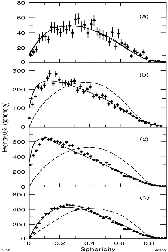
Figure 2: Sphericity distributions measured by the Mark I experiment at SPEAR [8] at c.m. energies of (a) 3.0, (b) 6.2, (c) 7.4 GeV. The narrowing of the distribution, and the trend towards smaller values as the c.m. energy is raised, represent evidence for collimated production of hadrons in e⁺e^- annihilation. The dashed line represents the expectation from a ‘phase-space model’ of hadron production. (d) As (c) but for a subset of events containing particles with scaled momentum, $2p/Q$, less than 0.4.

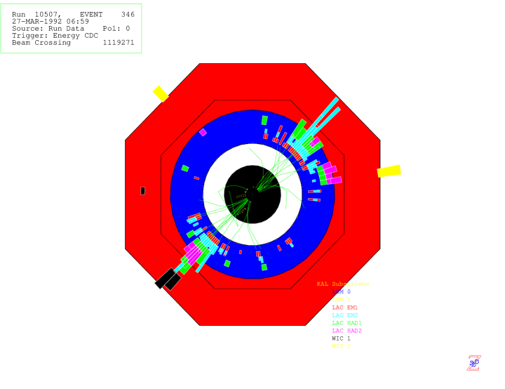
Figure 3: A contemporary two-jet event recorded by SLD: the process e⁺e^-$\rightarrow$$Z^{0}$ $\rightarrow$q$\overline{\rm q}$.

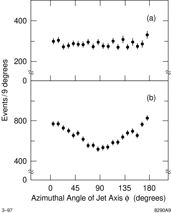
Figure 4: Azimuthal-angle distribution of the sphericity axis from Mark I [8]. At $Q$ = 6.2 GeV (a) the SPEAR beams were unpolarised and at $Q$ = 7.4 GeV (b) the polarisation-product was 0.47; the modulation in (b) is characteristic of the production of two spin-1/2 particles in e⁺e^- annihilation.

These studies were subsequently extended at the higher-energy PETRA collider, and examples from TASSO [12] are shown in Fig. 5. Here the distribution of the polar-angle ($\theta_{S}$) of the sphericity axis is shown at c.m. energies of 14, 22 and 35 GeV. A fit to the functional form:

$$\frac{dN}{d\cos\theta}\quad\propto\quad 1\;+\;a_{S,T}\cos^{2}\theta_{S,T}$$ (7)

yields, at 35 GeV for example, $a_{S}$ = $1.03\pm 0.07$, again characteristic of the production of two spin-1/2 particles in the e⁺e^- annihilation. Also shown in Fig. 5 is our second example of an event shape observable in the form of the thrust-axis [13] polar-angle ($\theta_{T}$) distribution. Thrust will be discussed later; it is qualitatively similar to sphericity in that it can be used to quantify the degree of collimation of particle production, although it has properties that make it more attractive theoretically. The thrust-axis polar-angle distribution in Fig. 5 was fitted to obtain, at 35 GeV for example, $a_{T}$ = $1.01\pm 0.06$, in good agreement with the result using the sphericity axis.

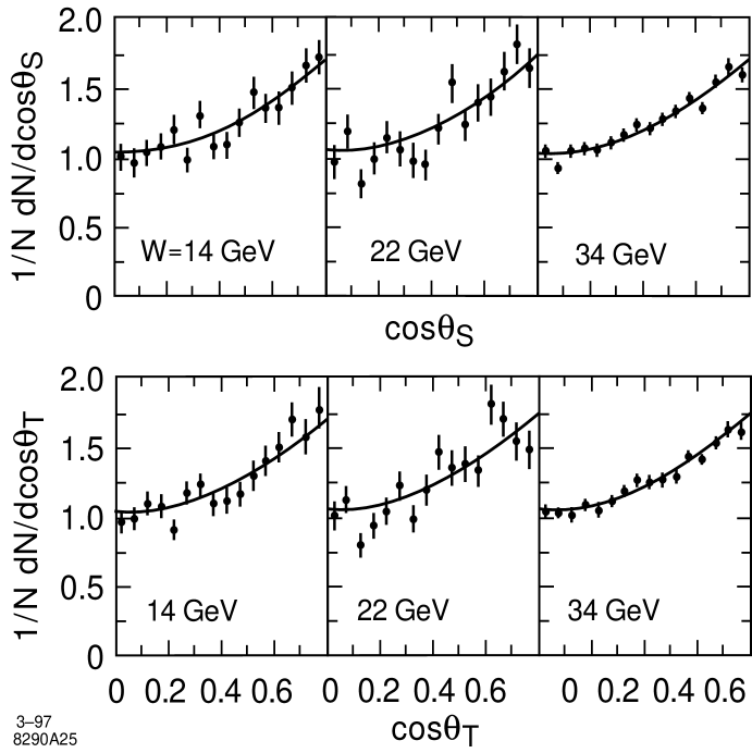
Figure 5: Polar-angle distributions of the sphericity and thrust axes from TASSO [12]. The $1+\cos^{2}\theta$ form is characteristic of the production of two spin-1/2 particles in the e⁺e^- annihilation.

So far spin-1/2 quarks and antiquarks would appear to be well established, and their colour-triplet nature, $N_{C}$ = 3, is required in the quark-parton model (QPM) of hadrons to explain the existence of spin-3/2 baryon states such as the $\Delta^{++}$ (u$\uparrow$u$\uparrow$u$\uparrow$) and $\Omega^{-}$ (s$\uparrow$s$\uparrow$s$\uparrow$), which would otherwise contain three identical fermions in the same quantum state, in violation of the Pauli exclusion principle. In e⁺e^- annihilationevidence for $N_{C}=3$ is provided by the quantity:

$$R\quad\equiv\quad\frac{\sigma(e^{+}e^{-}\;\rightarrow\;{\rm hadrons})}{\sigma_{QED}(e^{+}e^{-}\;\rightarrow\;\mu^{+}\mu^{-})}$$

which, according to QED and the QPM, should be equal to $N_{C}\;\Sigma_{f}\;q_{f}^{2}$, where $q_{f}$ is the charge of the quark of flavour $f$ and the sum runs over all active flavours at a given c.m. energy.

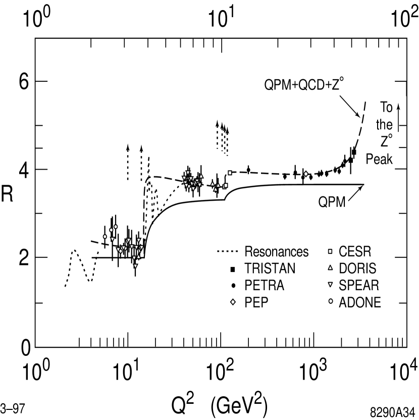
Figure 6: The $R$ ratio as a function of c.m. energy [14]. The expectation for $N_{C}$ = 3 is shown as the solid line.

A summary of $R$ measurements made up to 1988, as a function of c.m. energy, is presented in Fig. 6 [14]. This is a tremendously information-rich figure. First, increases in $R$ just above $Q^{2}$ = 10 and 100 GeV² represent the ${\rm c}\bar{\rm c}$ and ${\rm b}\bar{\rm b}$ production thresholds - further evidence, were it needed, for the existence of quarks. Secondly, the QED + QPM prediction comes close to the data only if the quarks are assigned fractional charges and the number of colours $N_{C}$ = 3 is used; the ‘colour singlet’ expectation ($N_{C}$ = 1) is simply too low by a factor of about three! Thirdly, above $Q^{2}$ = 1000 GeV² the data points rise as $Q^{2}$ increases, representing the onset of contributions to e⁺e^- annihilationfrom $Z^{0}$ exchange. Finally, in regions between quark flavour thresholds and below the tail of the $Z^{0}$ resonance, there is a residual excess in the data relative to the QED + QPM expectation, and the excess appears to decrease as $Q^{2}$ increases. In other words, some mechanism causes an increase in the ‘phase-space’ for hadron production beyond QED + QPM, but at a rate that decreases with $Q^{2}$. In the language of the 1990s we know that the extra contribution is due to gluon emission in the final state, and that the probability for this process, $\alpha_{s}$, decreases roughly logarithmically with $Q^{2}$. The $R$-ratio thus provides indirect evidence for the existence of the gluon, as well as for the non-Abelian ‘running’ of the strong coupling.

3.2 Three-Jet Events and the Gluon

In e⁺e^-annihilation events containing three distinct jets of hadrons were first observed in 1979 at the PETRA storage ring [15] at c.m. energies around 20 GeV. Such events were interpreted [16] in terms of the fundamental process e⁺e^-$\rightarrow$q$\overline{\rm q}$g , providing direct evidence for the existence of the gluon and its coupling to quarks. A modern example of a three-jet event, in fact the very event used to advertise this Summer Institute, is shown in Fig. 7.

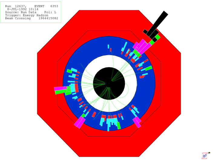
Figure 7: A contemporary three-jet event recorded by SLD: the process e⁺e^-$\rightarrow$$Z^{0}$ $\rightarrow$q$\overline{\rm q}$g .

Counting the number of jets per event, and then comparing the numbers of two- and three-jet events, it was found [17] that around $Q$ = 20 GeV

$$\frac{\#{\rm 3-jet\;events}}{\#{\rm 2-jet\;events}}\quad\approx\quad 0.15.$$ (8)

Since, at lowest order in perturbative QCD, this ratio is simply the probability for gluon emission, or $\alpha_{s}$, the strong coupling parameter, simple event counting indicated that the strong coupling at 20 GeV was around 0.15, i.e.about ten times larger than the electromagnetic coupling $\alpha$. More systematic determinations of $\alpha_{s}$will be discussed later.

Having observed the gluon directly in three-jet events one still needs to know whether it is the gluon of QCD, namely a colour-octet vector particle. Many studies of the nature of the gluon spin were performed at the PETRA and PEP storage rings and involved analysis of the partition of energy among the three jets. Ordering the three jets in e⁺e^-$\rightarrow$q$\overline{\rm q}$g   according to their energies $E_{1}>E_{2}>E_{3}$, and normalising by the c.m. energy $Q$, we obtain the scaled jet energies

$$x_{i}\quad=\quad{2E_{i}\over Q}\quad\quad\quad(i=1,2,3),$$ (9)

represented in Fig. 8, where $x_{1}+x_{2}+x_{3}=2$. Making a Lorentz boost of the event into the rest frame of jets 2 and 3 the historically-important Ellis-Karliner angle $\theta_{EK}$ is defined [18] to be the angle between jets 1 and 2 in this frame. For massless partons at tree-level:

$$cos\theta_{EK}={{x_{2}-x_{3}}\over{x_{1}}}.$$ (10)

The results of an early study by TASSO [19] are shown in Fig. 9, where the Ellis-Karliner angle distribution is compared, for data taken at $Q$ $\sim$ 30 GeV, with the prediction of QCD. One can also consider alternative ‘toy’ models of strong interactions, for example a model incorporating spin-0 (scalar) gluons [20]. From Fig. 9 the scalar-gluon model is clearly excluded.

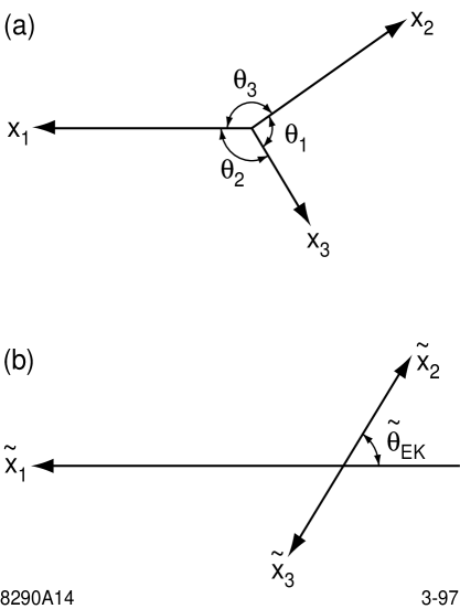
Figure 8: (a) Representation of the momentum vectors in a three-jet event, and (b) definition of the Ellis-Karliner angle.

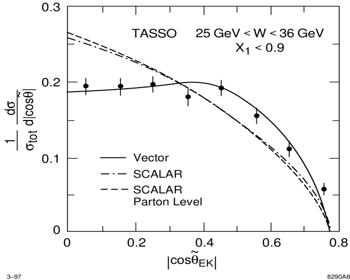
Figure 9: The Ellis-Karliner angle distribution of three-jet events recorded by TASSO at $Q$ $\sim$ 30 GeV [19]; the data favour spin-1 (vector) gluons.

Similar studies have been extended at the $Z^{0}$ resonance by the LEP and SLC experiments. In this case the inclusive differential cross sections, calculated at leading order and assuming massless partons, can be written for vector gluons [6]:

$${1\over\sigma}{d^{2}\sigma^{V}\over dx_{1}dx_{2}}\propto{{x_{1}^{3}+x_{2}^{3}+(2-x_{1}-x_{2})^{3}}\over{(1-x_{1})(1-x_{2})(x_{1}+x_{2}-1)}},$$ (11)

for scalar gluons [20]:

$${1\over\sigma}{d^{2}\sigma^{S}\over dx_{1}dx_{2}}\propto\biggl{[}{{x_{1}^{2}(1-x_{1})+x_{2}^{2}(1-x_{2})+(2-x_{1}-x_{2})^{2}(x_{1}+x_{2}-1)}\over{(1-x_{1})(1-x_{2})(x_{1}+x_{2}-1)}}-R\biggr{]},$$ (12)

where

$${R}={10\;{\Sigma_{j}a_{j}^{2}}\over{\Sigma_{j}(v_{j}^{2}+a_{j}^{2})}}$$ (13)

and $a_{j}$ and $v_{j}$ are the axial and vector couplings, respectively, of quark flavor $j$ to the $Z^{0}$, and for a model of strong interactions incorporating spin-2 (tensor) gluons [21, 22]:

$${1\over\sigma}{d^{2}\sigma^{T}\over dx_{1}dx_{2}}\propto{{(x_{1}+x_{2}-1)^{3}+(1-x_{1})^{3}+(1-x_{2})^{3}}\over{(1-x_{1})(1-x_{2})(x_{1}+x_{2}-1)}}.$$ (14)

Singly-differential cross sections for $x_{1}$, $x_{2}$, $x_{3}$ or cos$\theta_{EK}$ can be obtained by numerical integrations of Eqs. (11), (12) and (14) and are compared with SLD data [22] in Fig. 10. The shapes are different for the vector, scalar and tensor gluon cases and only the vector case describes the data.

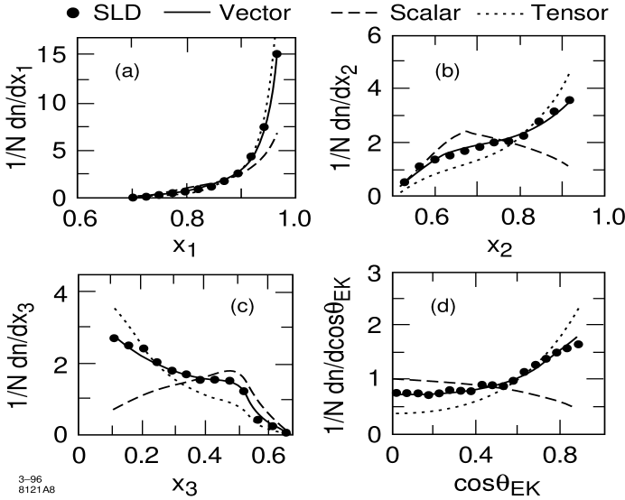
Figure 10: Comparison of leading-order scalar-, vector-, and tensor-gluon models with SLD data [22]; the scalar and tensor hypotheses are clearly excluded.

An additional interesting observable in three-jet events is the orientation of the event plane w.r.t. the beam direction, which can be described by three Euler angles (Fig. 11). These angular distributions were studied first by TASSO [23], and more recently by L3 [24] and DELPHI [25]. Again, the data were compared with the predictions of perturbative QCD and a scalar gluon model, but the Euler angles are less sensitive than the jet energy distributions to the differences between the two cases [24]. One can parametrise the angular distributions in the form:

$${d\sigma\over d{\rm cos}\theta}\quad\propto\quad 1\;+\;\alpha(T){\rm cos}^{2}\theta$$ (15)

$${d\sigma\over d{\rm cos}\theta_{N}}\quad\propto\quad 1\;+\;\alpha_{N}(T){\rm cos}^{2}\theta_{N}$$ (16)

$${d\sigma\over d\chi}\quad\propto\quad 1\;+\;\beta(T){\rm cos}2\chi$$ (17)

where $T$ is the thrust value [13] of the event. As an example, fits of eq. (16) to SLD distributions of cos$\theta_{N}$ are shown in Fig. 12 [22] in four bins of thrust. The coefficients $\alpha(T)$, $\alpha_{N}(T)$ and $\beta(T)$ depend on the gluon spin; they are shown in Fig. 13 for leading-order calculations incorporating vector, scalar and tensor gluons. The measured $\alpha(T)$, $\alpha_{N}(T)$ and $\beta(T)$ are also shown in Fig. 13 and confirm that only vector gluons are compatible with the data.

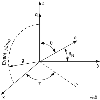
Figure 11: Definition of event-plane orientation angles.

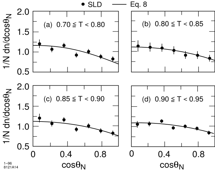
Figure 12: Distributions of cos$\theta_{N}$ as a function of event thrust from SLD [22].

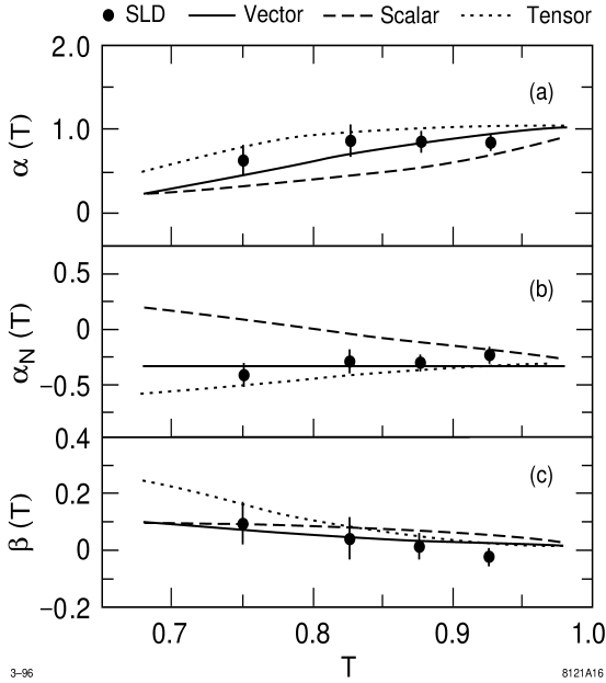
Figure 13: Dependence of the coefficients of the three-jet event plane orientation angular distributions on event thrust value [22].

At this point it is worth pausing to take stock of what has been learned so far. The e⁺e^-$\rightarrow$two-jet events have provided direct evidence for q$\overline{\rm q}$production, and the jet axis angular distribution indicates that the quark and antiquark have spin-1/2. From the inclusive $R$-ratio we can confirm the fractional nature of the quark charges, and know that the quarks must exist as colour triplets since $N_{C}$ = 3 is the only value that brings QED + the quark-parton model close to the data. The value of the $R$-ratio also tells us that there must be contributions to hadronic final states in addition to q$\overline{\rm q}$production, and we know that these are provided by three-jet events, which represent direct evidence for the existence of the gluon and its coupling to quarks and antiquarks. The distributions of jet energies, or equivalently of jet angles within the event plane, as well as of the event plane orientation itself, confirm that the only hypothesis that fits the data is that the gluon has spin-1, and therefore that it is the vector boson of QCD. Finally, from counting the relative rates of three- and two-jet events at $Q$ $\sim$ 30 GeV we know that the coupling strength of the gluon to quarks is about 0.15. Checking the list of ‘essential features’ of QCD we see that we have verified about half of them! The next item in the list refers to the triple- and quartic-gluon couplings; in order to study these we need to examine multi-jet final-states.

3.3 Multi-Jet Events and Gluon Self-Couplings

Consider the Feynman diagrams for production of 4-jet final states shown in Fig. 14. Figs. 14(a) and (b) illustrate the gluon Bremsstrahlung process, whilst Fig. 14(d) shows the splitting of a gluon into a quark and an antiquark; the latter may be thought of as a QCD analogue of the QED process whereby a photon converts into an electron and a positron. Figs. 14(a,b,d) are sometimes referred to as ‘Abelian’ diagrams. Fig. 14(c) illustrates the lowest-order diagram for a gluon to split into two gluons. This process has no analogue in QED since the photon does not couple to itself, and is a consequence of the non-Abelian nature of QCD in that the gluons, by virtue of possessing colour charge, can interact among themselves.

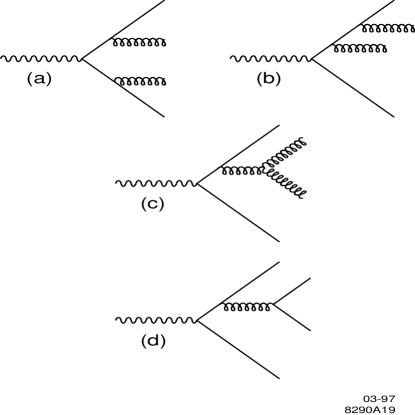
Figure 14: Tree-level Feynman diagrams for 4-jet production in e⁺e^- annihilation.

Now consider the formal properties of the SU(3) group. The group can be characterised by constants known as Casimir factors that are defined by:

$$\Sigma_{a}(T^{a}T^{a})_{ij}\quad=\quad\delta_{ij}C_{F}$$ (18)

$$\Sigma_{a,b}(f^{abc}f^{abd})\quad=\quad\delta^{cd}N_{C}$$ (19)

$$Tr[T^{a}T^{b}]\quad=\quad\delta^{ab}T_{F}$$ (20)

The Casimir factors for several common groups are shown in Table 2. We see that in the case of SU(3) $N_{C}$ corresponds to the now-familiar ‘number of colours’ that we have already encountered several times. The tree-level couplings appearing in Fig. 14 may be classified in terms of the Casimir factors, as illustrated in Fig. 15. The amplitude-squared corresponding to the Bremsstrahlung diagrams (Fig. 14(a,b)) is proportional to $C_{F}$, that corresponding to g $\rightarrow$q$\overline{\rm q}$is proportional to $T_{F}$, and that corresponding to the non-Abelian process g $\rightarrow$gg is proportional to $N_{C}$.

Group	$N_{C}$	$C_{F}$	$T_{F}$
U(1)	$0$	1	1
U(1)3	$0$	1	3
SU(N)	$N$	$(N^{2}-1)/2N$	1/2
SU(3)	$3$	4/3	1/2

Table 2: Casimir factors for some common gauge groups.

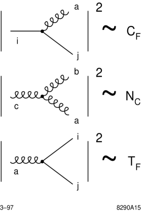
Figure 15: Casimir classification of tree-level QCD couplings.

It is interesting to consider whether the Casimir factors of SU(3) QCD can be measured. Clearly nature does not deliver events corresponding to the tree-level vertices shown in Fig. 15! Instead, one must write down the Feynman amplitudes for the 4-jet event diagrams shown in Fig. 14, add them to those for 2- and 3-jet production at the same order of perturbation theory, and square them to derive the total hadronic cross section. The terms corresponding to 4-jet production can then be identified in a gauge-invariant manner, and yield a differential cross section of the form:

$${1\over\sigma_{0}}d\sigma^{4}\quad=\quad\left({\alpha_{s}C_{F}\over\pi}\right)^{2}\left[F_{A}+\left(1-{1\over 2}{N_{C}\over C_{F}}\right)F_{B}+{N_{C}\over C_{F}}F_{C}\right]$$

$$\quad\quad\quad+\quad\left({\alpha_{s}C_{F}\over\pi}\right)^{2}\left[{T_{F}\over C_{F}}N_{f}F_{D}+\left(1-{1\over 2}{N_{C}\over C_{F}}\right)F_{E}\right]$$ (21)

where $F_{A}$ $\dots$ $F_{E}$ are kinematical functions. We see that the overall normalisation of the cross-section is proportional to $(\alpha_{s}\,C_{F})^{2}$, and that the kinematical distribution of the four jets depends on the ratios $N_{C}/C_{F}$ and $T_{F}/C_{F}$, which can hence in principle be measured.

The issue of jet definition will be discussed in detail in Section 4.4. For now let us assume that 4-jet events can be defined and measured in particle detectors, and that they can be related meaningfully to the underlying 4-jet parton structure described by eq. (21). Two important physical characteristics underly the definition of 4-jet observables that are sensitive to $N_{C}/C_{F}$ and $T_{F}/C_{F}$: the first is that the two jets resulting from the primary quark and antiquark produced in the $Z^{0}$ decay tend to be more energetic than the jets produced by the two radiated gluons or the radiated q$\overline{\rm q}$; the second is that in the ‘non-Abelian’ process (Fig. 14c) the two gluons tend to be produced in the plane of the primary quark and antiquark, whereas in the ‘Abelian’ process (Fig. 14d) the radiated quark and antiquark tend to be produced along an axis normal to this plane [26].

With this in mind, a number of 4-jet observables that are potentially sensitive to the ratios of Casimir factors have been proposed over the years. If one orders and labels the four jets in an event in terms of their momenta (or energies) such that $p_{1}>p_{2}>p_{3}>p_{4}$ one can define the Bengtsson-Zerwas angle [27] (Fig. 16):

$$\cos\chi_{BZ}\quad\propto\quad(\vec{p_{1}}\times\vec{p_{2}})\cdot(\vec{p_{3}}\times\vec{p_{4}})$$ (22)

and the Nachtmann-Reiter angle [26] (Fig. 17):

$$\cos\theta^{*}_{NR}\quad\propto\quad(\vec{p_{1}}-\vec{p_{2}})\cdot(\vec{p_{3}}-\vec{p_{4}}).$$ (23)

The sensitivity of these observables is illustrated in Fig. 18, where the distributions of these angles are shown for SU(3) QCD, as well as for a straw-person U(1)₃ Abelian model of strong interactions, and are compared with L3 data [28]; the Abelian model is clearly excluded.

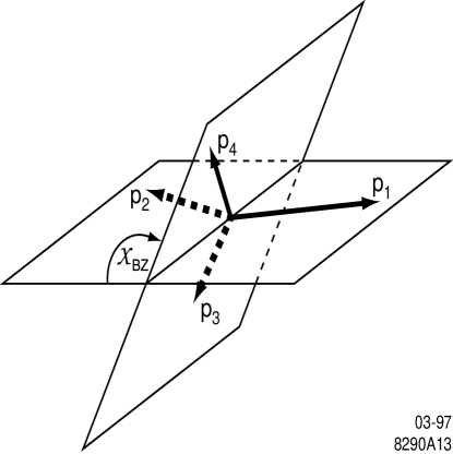
Figure 16: Definition of the Bengtsson-Zerwas angle.

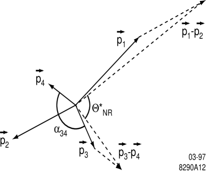
Figure 17: Definition of the Nachtmann-Reiter angle.

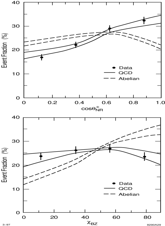
Figure 18: Illustration of the sensitivity of the Nachtmann-Reiter and Bengtsson-Zerwas angles to non-Abelian effects and comparison with L3 data [28].

A more recent analysis by OPAL [29] is summarised in Fig. 19; here a simultaneous fit was performed to the Nachtmann-Reiter and Bengtsson-Zerwas angle distributions, as well as to the angle $\alpha_{34}$ between jets 3 and 4. The resulting values of $N_{C}/C_{F}$ and $T_{F}/C_{F}$ are displayed in Fig. 20, where they are compared with the expectations from numerous gauge groups. The SU(3) QCD expectation is clearly in good agreement with the data. The expectations from several other gauge models, such as SU(4), Sp(4) and Sp(6), also appear to be compatible with the experimental results. Note, however, that none of these models contains three colour degrees of freedom for quarks, and hence all can be ruled out on that basis. Besides SU(3), only the U(1)₃ and SO(3) models contain three quark colours, but both are inconsistent with the measured values of $N_{C}/C_{F}$ and $T_{F}/C_{F}$. The results shown in Fig. 20 hence yield the remarkable conclusion that SU(3) is the only known viable gauge model for strong interactions.

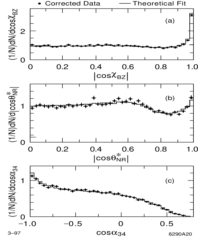
Figure 19: Simultaneous fit of QCD to OPAL measurements of $\chi_{BZ}$, $\theta_{NR}$ and $\alpha_{34}$ [29].

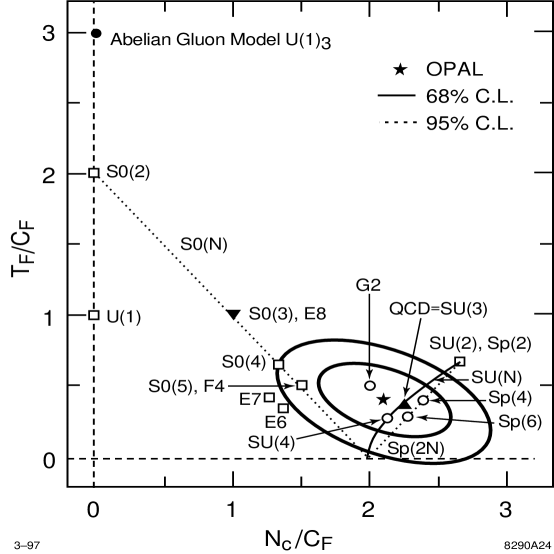
Figure 20: The $T_{F}/C_{F}$ vs. $N_{C}/C_{F}$ plane showing the fitted values derived from Fig. 19, as well as the expectations from numerous gauge groups [29]; QCD is in good agreement with the data.

Recalling the ‘essential feature’ of QCD that the ggg vertex must exist, we see from Fig. 20 that the non-zero measured value of $N_{C}/C_{F}$ provides direct evidence for its contribution to 4-jet production. Now consider the existence of the gggg vertex; it should come as no surprise that we need to study events of yet higher jet multiplicity in order to be sensitive to it. The tree-level Feynman diagrams for 5-jet production in e⁺e^- annihilationare shown in Fig. 21; the gggg vertex can be seen in the two diagrams just left of centre on the bottom row.

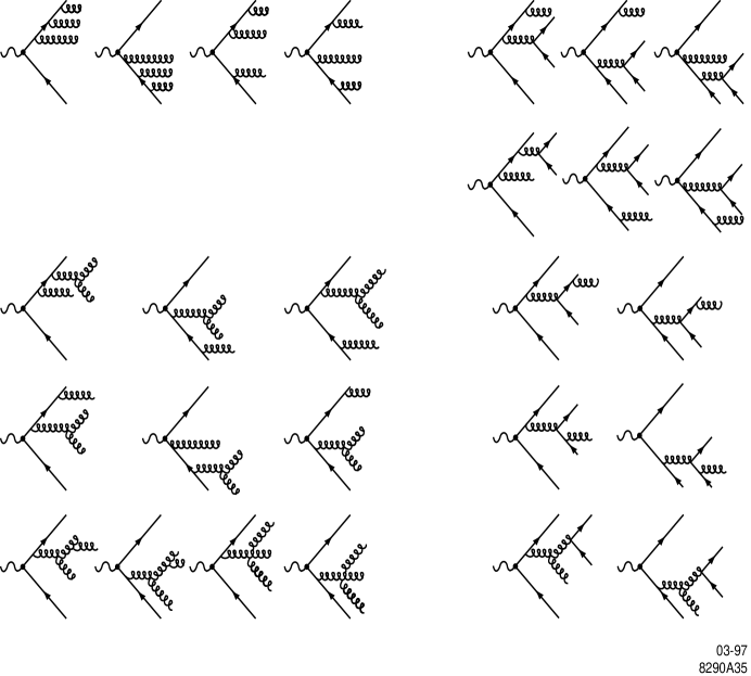
Figure 21: Tree-level Feynman diagrams for 5-jet production in e⁺e^- annihilation.

Performing a similar exercise to that for the 4-jet cross section one finds:

$${1\over\sigma_{0}}d\sigma^{5}\quad=\quad{1\over\sigma_{0}}d\sigma^{2q3g}\quad+\quad{1\over\sigma_{0}}d\sigma^{4q1g},$$ (24)

The first term contributes about 85% of the 5-jet cross section, and may be written:

$${1\over\sigma_{0}}d\sigma^{2q3g}\quad=\quad\left({\alpha_{s}C_{F}\over\pi}\right)^{3}\left[\;G_{A}\quad+\quad{N_{C}\over C_{F}}G_{B}\quad+\quad\left({N_{C}\over C_{F}}\right)^{2}G_{C}\;\right]$$ (25)

where $G_{A}$, $G_{B}$ and $G_{C}$ are kinematical functions. The contribution of the gggg vertex is represented by the last term in eq. (25), which is proportional to $(N_{C}/C_{F})^{2}$. We have just seen that $N_{C}/C_{F}$ must be non-vanishing in order to describe the 4-jet data, so that the existence of the gggg vertex is absolutely required in QCD in order for the theory to be gauge-invariant and self-consistent. Pushing pedagogy to its limits, however, one can still ask if the data actually require the existence of the gggg vertex, from a phenomenological point-of-view. One can therefore define a set of ad hoc5-jet correlation observables, such as those illustrated in Fig. 22 [30]. The measured distributions of the five of these observables that are most sensitive to the $(N_{C}/C_{F})^{2}$ term are shown in Fig. 23, from the OPAL Collaboration [30].

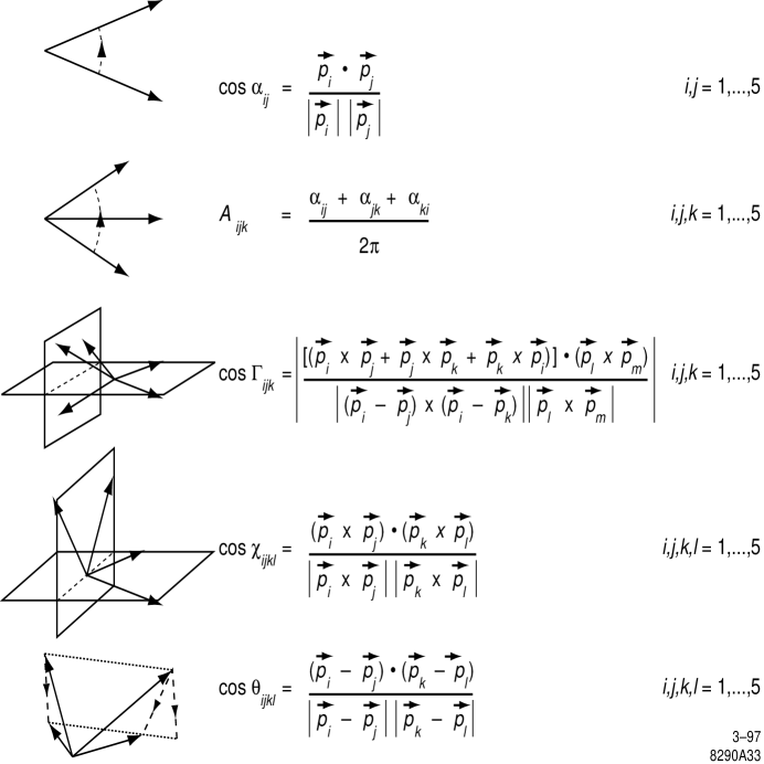
Figure 22: Illustration of correlation observables among the jets in 5-jet events [30].

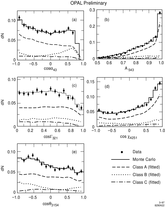
Figure 23: The five correlation observables in 5-jet events that are most sensitive to contributions from the gggg vertex [30].

Two possible strategies now present themselves for testing the self-consistencey of QCD. One could fit inclusively the quantity $N_{C}/C_{F}$ to the 5-jet data shown in Fig. 23 and compare it with the value determined from 4-jet events; the results of such a comparison are shown in Fig. 24a; the 4-jet and 5-jet events clearly yield consistent results. A second possibility is to fit phenomenologically only the gggg contribution proportional to $(N_{C}/C_{F})^{2}$; the results are shown in Fig. 24b. In the latter case the error bars are large due to the small number of 5-jet events, as well as to the large uncertainties on multijet production that arise from hadronisation effects (see Section 4.4). The measured value of $(N_{C}/C_{F})^{2}$ is clearly consistent with the QCD expectation of $(9/4)^{2}$ $\approx$ 5, but it is also consistent with zero, so that the existence of the gggg vertex has not yet been established from a phenomenological point-of-view.

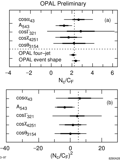
Figure 24: Measurements of (a) $(N_{C}/C_{F})$ and (b) $(N_{C}/C_{F})^{2}$ made using 5-jet events at OPAL [30].

3.4 Review of Strategy for QCD Tests

At this point we have seen that most of the ‘essential features’ of QCD have been established empirically, with the possible exception of the gggg coupling. Even in this case, given the existence of the ggg vertex, the gggg vertex must exist in QCD in order for the theory to be gauge-invariant. The last 20 years of hadronic-event studies at e⁺e^-colliders have hence established, in a qualitative sense, that the QCD Lagrangian is the correct one to describe strong interactions. At this point it therefore seems sensible to revise the strategy for testing QCD.

Since the theory contains in principle only one free parameter, the strong coupling $\alpha_{s}$, QCD can be tested in a quantitative fashion by measuring $\alpha_{s}$in different processes and at different hard scales $Q$. The precision of these measurements, and the resulting degree of consistency among them, determine quantitatively the precision with which the theory has been tested. This philosophy is directly analogous to that used to test the electroweak theory by measuring a large number of observables that are sensitive to a few key unknown parameters of the theory. In addition to testing QCD, the precise measurement of $\alpha_{s}$allows constraints on possible extensions to the Standard Model (SM) of elementary particles; see eg.[31]. Measurements of $\alpha_{s}$have been performed in e⁺e^- annihilation, hadron-hadron collisions, and deep-inelastic lepton-hadron scattering, covering a range of $Q^{2}$ from roughly 1 to $10^{5}$ GeV². In the next section I shall describe the e⁺e^-measurements, and compare them with those made in other hard processes; for a review of this field see [32].

4. Measurements of $\alpha_{s}$in e⁺e^-Annihilation

4.1 Theoretical Considerations

An inclusive observable $X$ may be written schematically:

$$X\quad=\quad X^{EW}\;(1\;+\;\delta^{QCD})$$ (26)

where $X^{EW}$ represents the electroweak contribution. Since, with observables of this type, $\alpha_{s}$enters via the small QCD radiative correction, $\delta^{QCD}$, a precise measurement of $\alpha_{s}$generally requires a large data sample. Observables can also be defined that are directly proportional to $\delta^{QCD}$ and hence potentially more sensitive to $\alpha_{s}$. In either case $\delta^{QCD}$ can be separated into perturbative and non-perturbative contributions:

$$\delta^{QCD}\quad=\quad\delta^{pert}+\delta^{non-pert}.$$ (27)

The perturbative contribution can in principle be calculated as a power series in $\alpha_{s}$, though in practice the large number of Feynman diagrams involved renders a complete calculation beyond the first few orders intractable. The non-perturbative contribution, often called a ‘hadronisation correction’ in e⁺e^- annihilationor a ‘higher twist effect’ in lepton-hadron scattering, is expected to have the form of a series of inverse powers of the physical scale (see section 5).

In practice most QCD calculations of observables are performed using finite-order perturbation theory, and calculations beyond leading order depend on the renormalisation scheme employed, implying a scheme-dependent strong-interaction scale $\Lambda$. It is conventional to work in the modified minimal subtraction scheme ($\overline{MS}$ scheme) [33], and to use the strong interaction scale $\Lambda_{\overline{MS}}$for five active quark flavours. If one knows $\Lambda_{\overline{MS}}$one may calculate the strong coupling $\alpha_{s}$($Q^{2}$) from the solution of the QCD renormalisation group equation [34]:

$$\alpha_{s}(Q^{2})\quad=\quad{4\pi\over{\beta_{0}{\rm ln}(Q^{2}/\Lambda_{\overline{MS}}^{2})}}\{\;1\;-\;{2\beta_{1}\over\beta_{0}^{2}}\;{{\rm ln(ln}(Q^{2}/\Lambda_{\overline{MS}}^{2}))\over{\rm ln}(Q^{2}/\Lambda_{\overline{MS}}^{2})}\;+\ldots\;\}$$ (28)

Because of the large data samples taken in e⁺e^- annihilationat the $Z^{0}$ resonance, it has become conventional to use as a yardstick $\alpha_{s}(M_{Z}^{2})$, where $M_{Z}$ is the mass of the $Z^{0}$ boson; $M_{Z}$ $\approx$ 91.2 GeV [35]. Tests of QCD can therefore be quantified in terms of the consistency of the values of $\alpha_{s}(M_{Z}^{2})$measured in different experiments. The ‘QCD-challenged’ reader may like to think of $\alpha_{s}(M_{Z}^{2})$as being ‘the sin${}^{2}\theta_{W}$ of strong interactions’.

In e⁺e^- annihilation$\alpha_{s}(M_{Z}^{2})$has been measured from inclusive observables relating to the $Z^{0}$ lineshape and to hadronic decays of the $\tau$ lepton, as well as from jet-related hadronic event shape observables, and scaling violations in inclusive hadron fragmentation functions.

4.2 $R$ and the $Z^{0}$ Lineshape

For the inclusive ratio $R$ = $\sigma$(e⁺e^-$\rightarrow$hadrons)/$\sigma$(e⁺e^-$\rightarrow$$\mu^{+}\mu^{-}$), the SM electroweak contributions are well understood theoretically and the perturbative QCD series has been calculated up to O($\alpha_{s}^{3}$)[36] for massless quarks and up to O($\alpha_{s}^{2}$)including quark mass effects [37]; the large size of the O($\alpha_{s}^{3}$)term is potentially a cause for concern about the degree of convergence of the series. Closely-related observables at the $Z^{0}$ resonance are:

$\bullet$ the $Z^{0}$ total width, $\Gamma_{Z}$

$\bullet$ the pole cross section, $\sigma_{h}^{0}\;\equiv\;12\pi\Gamma_{ee}\Gamma_{had}/{M_{Z}^{2}\Gamma_{Z}^{2}}$

$\bullet$ the ratio of hadronic to leptonic $Z^{0}$ decay branching ratios $R_{l}\;\equiv\;\Gamma_{had}/\Gamma_{ll}$

which all depend on the $Z^{0}$ hadronic width:

$$\Gamma_{had}\quad=\quad 1.671\left(1\;+\;a_{1}\left({\alpha_{s}\over\pi}\right)\;+\;a_{2}\left({\alpha_{s}\over\pi}\right)^{2}\;+\;a_{3}\left({\alpha_{s}\over\pi}\right)^{3}\;+\quad\ldots\right)$$ (29)

where: $a_{1}$ = 1, $a_{2}$ = 0.75 and $a_{3}$ = $-15.3$. In these cases the non-perturbative contributions are expected to be O(1/$M_{Z}$) and are usually ignored. A concern is that recent measurements of observables that probe the electroweak couplings of the $Z^{0}$ to b and c quarks deviate slightly from SM expectations [38]. Since these couplings must be known in order to extract $\alpha_{s}(M_{Z}^{2})$, this effect, whatever its origin, is a potential source of bias [34]. Further analysis is in progress from the SLC and LEP experiments and the situation is not yet resolved.

Proceeding nonetheless, the procedure adopted [38] is to perform a global SM fit to a panoply of electroweak data that includes the W and top quark masses as well as the $Z^{0}$ observables relating to the lineshape, left-right production asymmetry, decay fermion forward-backward asymmetries, branching ratios to heavy quarks, and $\tau$ polarisation. The free parameters are the Higgs mass, $M_{Higgs}$, which contributes to $X^{EW}$, and $\alpha_{s}(M_{Z}^{2})$. Data presented at the 1996 summer conferences yield the results shown in Fig. 25 [38], from which the positively-correlated results $M_{Higgs}=149^{+190}_{-82}$ GeV and

$$\alpha_{s}(M_{Z}^{2})\quad=\quad 0.1202\pm 0.0033\;\;({\rm exp.})$$ (30)

are obtained. The $\alpha_{s}(M_{Z}^{2})$value is lower than the corresponding results presented at the 1995 conferences [39], $\alpha_{s}(M_{Z}^{2})$= $0.123\pm 0.005$, and at the 1994 conferences, $\alpha_{s}(M_{Z}^{2})$$0.125\pm 0.005$ [40], whose large central values were partly responsible for a supposed discrepancy between ‘low-$Q^{2}$’ and ‘high-$Q^{2}$’ $\alpha_{s}(M_{Z}^{2})$measurements [41]. The change between 1995 and 1996 is due to a combination of shifts in the values of the $Z^{0}$ lineshape parameters, redetermined in light of the recalibration of the LEP beam energy due to the ‘TGV effect’ [38], and a change in the central value of $M_{Higgs}$ at which $\alpha_{s}(M_{Z}^{2})$is quoted, from 300 GeV (1995) to the fitted value 149 GeV (1996). A detailed study of theoretical uncertainties implies [42] that they contribute at a level substantially below $\pm 0.001$. Since data-taking at the $Z^{0}$ resonance has now been completed at the LEP collider the precision of this result is not expected to improve further.

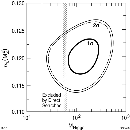
Figure 25: Results of a global fit of the Standard Model to electroweak observables [38]; the 1- and 2-standard deviation contours are shown in the $\alpha_{s}(M_{Z}^{2})$vs. $M_{Higgs}$ plane.

4.3 Hadronic $\tau$ Decays

An inclusive quantity similar to $R$ is the ratio $R_{\tau}$ of hadronic to leptonic decay branching ratios, $B_{h}$ and $B_{l}$ respectively, of the $\tau$ lepton:

$$R_{\tau}\quad\quad\equiv\quad{B_{h}\over B_{l}}\quad=\quad{1-B_{e}-B_{\mu}\over B_{e}}$$ (31)

where $B_{e}$ and $B_{\mu}$ can either be measured directly, or deduced from a measurement of the $\tau$ lifetime $\tau_{\tau}$. In addition, a family of observables known as ‘spectral moments’ of the invariant mass-squared $s$ of the hadronic system has been proposed [43]:

$$R_{\tau}^{kl}\quad\equiv\quad{1\over B_{e}}\int_{0}^{M_{\tau}^{2}}ds\left(1-{s\over M_{\tau}^{2}}\right)^{k}\left({s\over M_{\tau}^{2}}\right)^{l}{dB_{h}\over ds}$$ (32)

where $M_{\tau}$ is the $\tau$ mass. In this case the integrand can be measured independently of $B_{e}$. It is easily seen that $R_{\tau}$ = $R_{\tau}^{00}$.

$R_{\tau}$ and $R_{\tau}^{kl}$ have been calculated perturbatively up to O($\alpha_{s}^{3}$). However, because $M_{\tau}$ $\sim$ 1 GeV one expects (eq. (28)) $\alpha_{s}$($M_{\tau}$) $\sim$ 0.3 and it is not a prioriobvious that the perturbative calculation can be expected to be reliable, or that the non-perturbative contributions of O($1/M_{\tau}$) will be small. In recent years a large theoretical effort has been devoted to this subject; see eg.[43, 44, 45].

The ALEPH Collaboration derived $R_{\tau}$ from its measurements of $B_{e}$, $B_{\mu}$, and $\tau_{\tau}$, and also measured the (10), (11), (12), and (13) spectral moments. A combined fit yielded [46] $\alpha_{s}(M_{Z}^{2})$= $0.124\pm 0.0022\pm 0.001$, where the first error receives equal contributions from experiment and theory, and the second derives from uncertainties in evolving $\alpha_{s}$across the c and b thresholds. The OPAL Collaboration measured $R_{\tau}$ from $B_{e}$, $B_{\mu}$, and $\tau_{\tau}$, and derived [47] $\alpha_{s}(M_{Z}^{2})$=0.1229${}^{+0.0016}_{-0.0017}$ (exp.) ${}^{+0.0025}_{-0.0021}$ (theor.). The CLEO Collaboration measured the same four spectral moments as ALEPH and also derived $R_{\tau}$ using 1994 Particle Data Group values for $B_{e}$, $B_{\mu}$ and $\tau_{\tau}$. A combined fit yielded [48] $\alpha_{s}(M_{Z}^{2})$= $0.114\pm 0.003$. This central value is slightly lower than the ALEPH and OPAL values. If more recent world average values of $B_{e}$ and $B_{\mu}$ are used CLEO obtains a higher central $\alpha_{s}(M_{Z}^{2})$value [48]. Averaging the second CLEO result and the ALEPH and OPAL results by weighting with the experimental errors, assuming they are uncorrelated, yields:

$$\alpha_{s}(M_{Z}^{2})\quad=\quad 0.122\pm 0.001\;\;({\rm exp.})\;\;\pm 0.002\;\;({\rm theor.}).$$ (33)

This is nominally a very precise measurement, although recent studies have ruggested that additional theoretical uncertainties may be as large as $\pm 0.006$ [49].

4.4 Hadronic Event Shape Observables

As discussed in Section 3.2, in e⁺e^- annihilationthe rate of 3-jet production:

$$R_{3}\quad\equiv\quad\frac{\sigma_{3-jet}}{\sigma_{had}}$$ (34)

is directly proportional to $\alpha_{s}$and can hence be used to determine $\alpha_{s}$. In order to make a meaningful measurement that can be compared with those just discussed one must calculate $R_{3}$ to at least next-to-leading order in $\alpha_{s}$, i.e.to O($\alpha_{s}^{2}$). The relevant contributing Feynman diagrams are shown in Fig. 26; these form the basis of the O($\alpha_{s}^{2}$)calculation of $R_{3}$ [50, 51, 52].

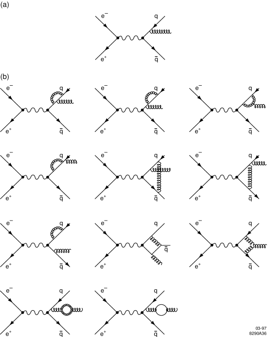
Figure 26: Tree-level and one-loop Feynman diagrams that contribute to 3-jet observables up to O($\alpha_{s}^{2}$)in QCD perturbation theory.

4.4.1 Definition of Jets and Event Shape Measures

The task is, in principle, straightforward. One must count the number of 3-jet events and divide by the total number of hadronic events to obtain $R_{3}$, then compare with the theoretical prediction to obtain $\alpha_{s}$. However, it is immediately apparent that one cannot simply define the jet multiplicity of events on the basis of a visual inspection! On the experimental side, the classic ‘Mercedes-Benz’ 3-jet event measured in a detector is rather rare; many events contain broad particle flows that might be classified as a single jet by one observer but as two or more jets by another observer. Moreover, in QCD the Bremsstrahlung spectrum of parton radiation peaks at small angles and is continuous. Hence even theoretically the issue of when a radiated parton is sufficiently energetic, and at a sufficiently wide angle relative to its parent, so as to be resolved as a separate jet is not without ambiguity. After due Cartesian deliberation one pragmatically concludes that one needs an algorithmic definition of a jet that can be applied to hadrons recorded in a detector, as well as to partons in perturbative QCD calculations, and a sensible recipe to translate between the two.

A convenient solution is provided by iterative clustering algorithms in which a measure $y_{ij}$, such as invariant mass-squared/$Q^{2}$, is calculated for all pairs of particles $i$ and $j$ in an event, and the pair with the smallest $y_{ij}$ is combined into a single ‘particle’. This process is repeated until all pairs have $y_{ij}$ exceeding a value $y_{c}$, and the jet multiplicity of the event is defined as the number of particles remaining. For a sample of events the $n$-jet rate $R_{n}$ is then defined as the number of $n$-jet events divided by the total number of events. This number is not a constant, but rather depends on the choice of algorithm and on the $y_{c}$ value. The $y_{c}$-dependence is illustrated in Fig. 27 for jets defined using the JADE algorithm [53] applied to SLD data [54]. One can think of $y_{c}$ as the ‘jet resolution’ scale. Large $y_{c}$ values correspond to poor eyesight, most events look 2-jet-like, and hence $R_{2}$ $\approx$ 1. Small $y_{c}$ values correspond to good eyesight, a richer jet structure is discernible, and $R_{3}$ and $R_{4}$ are non-zero. It should be noted, however, that from an operational point-of-view the data points shown in Fig. 27 are awkward to handle in that they are correlated between different $y_{c}$ values. A more convenient observable is the differential 2-jet rate:

$$D_{2}(y_{c})\;\equiv\;(R_{2}(y_{c})-R_{2}(y_{c}-\Delta y_{c}))/\Delta y_{c}$$ (35)

which is a measure of the rate of events that change their classification between 2-jet-like and $\geq 3$-jet-like as $y_{c}$ is varied across the range $\Delta y_{c}$. $D_{2}(y_{c})$ is illustrated in Fig. 28.

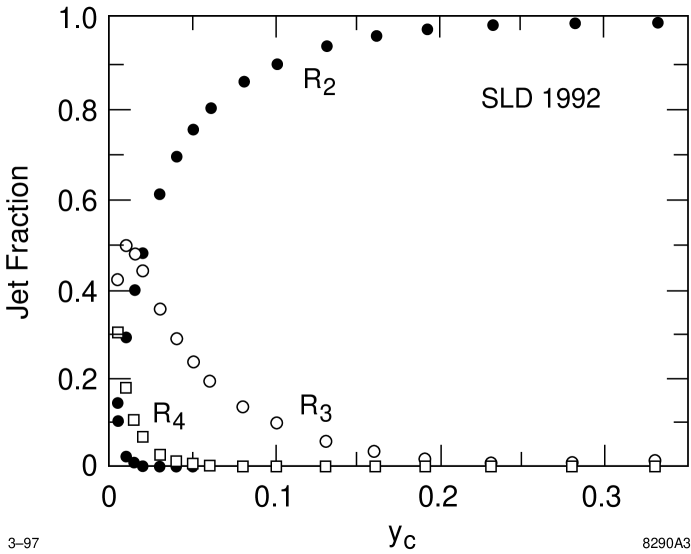
Figure 27: Dependence on the jet resolution parameter $y_{c}$ of the $n$-jet rates $R_{n}$ measured using SLD data [54] with the JADE algorithm.

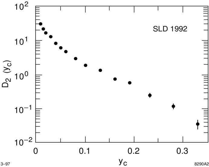
Figure 28: Dependence on the jet resolution parameter $y_{c}$ of the differential 2-jet rate $D_{2}$ [54].

In fact several variations of the JADE algorithm have been suggested [55]; these differ in the definition of the resolution measure $y_{ij}$, and/or in the ‘recombination scheme’ prescription for combining two particles that are unresolvable. A full discussion is beyond the scope of these lectures, but it is important to note that the ‘E’, ‘E0’, ‘P’ and ‘P0’ variations of the JADE algorithm, as well as the ‘Durham’ (‘D’) and ‘Geneva’ (‘G’) algorithms, are all collinear- and infra-red-safe observables, which, for our purposes, means that they can be calculated in perturbative QCD [56].

More generally one can define other infra-red- and collinear-safe measures of the topology of hadronic final states; a list of 15 such observables is given in Table 3. Thrust has already been encountered in Section 3 and is related to the longitudinal momentum flow in events:

$$T=\mbox{max}\frac{\sum_{i}\mid\vec{p}_{i}\cdot\vec{n}_{T}\mid}{\sum_{i}\mid\vec{p}_{i}\mid},$$ (36)

where $\vec{p}_{i}$ is the momentum vector of particle $i$, and $\vec{n}_{T}$ is the thrust axis to be determined. It is useful to define $\tau\equiv 1-T$. For back-to-back two-parton final states $\tau$ is zero, while $0\leq\tau\leq\frac{1}{3}$ for planar three-parton final states. Spherical events have $\tau=\frac{1}{2}$. An axis $\vec{n}_{maj}$ can be found to maximize the momentum sum transverse to $\vec{n}_{T}$, and an axis $\vec{n}_{min}$ is defined to be perpendicular to the two axes $\vec{n}_{T}$ and $\vec{n}_{maj}$. The variables thrust-major $T_{maj}$ and thrust-minor $T_{min}$ are obtained by replacing $\vec{n}_{T}$ in Eq. (36) by $\vec{n}_{maj}$ or $\vec{n}_{min}$, respectively. The oblateness $O$ is then defined by [57]

$$O=T_{maj}-T_{min}.$$ (37)

Other measures are related to jet masses, and energy-energy correlations between particles; for a discussion see eg.[58].

Observable	symbol
1 – Thrust	$\tau$
Heavy jet mass	$\rho$
Jet broadening:
Total	$B_{T}$
Wide	$B_{W}$
Oblateness	$O$
C-parameter	$C$
Differential jet rates:
$\quad D_{2}(y_{c})$ = ${\Delta R_{2}(y_{c})\over{\Delta y_{c}}}$	E
	E0
	P
	P0
	D
	G
Energy-energy correlations	$EEC$
Asymmetry of EEC	$AEEC$
Jet cone energy fraction	$JCEF$

Table 3: Fifteen infra-red- and collinear-safe measures of the topology of e⁺e^-hadronic final states.

The observables are all constructed to be directly proportional to $\alpha_{s}$at leading order, and so are potentially sensitive measures of the strong coupling. The O($\alpha_{s}^{2}$)QCD prediction for each of these observables $X$ can be written [52]:

$${1\over\sigma_{0}}{{\rm d}\sigma\over{\rm d}X}\quad=\quad A(X)\;\left({\alpha_{s}\over 2\pi}\right)\quad+\quad B(X)\left({\alpha_{s}\over 2\pi}\right)^{2}$$ (38)

so that $\alpha_{s}$can be determined from each. Though these observables are intrinsically highly correlated, by using all 15 to study $\alpha_{s}$one is attempting to maximise the use of the information in complicated multi-hadron events, and in some sense is making a more demanding test of QCD than by using only one or two observables. Moreover, it will be seen that the study of many observables is essential, as it may expose systematic effects. Finally, the $\alpha_{s}$determination from hadronic event shape observables is based on the information content within 3-jet-like events, and is essentially uncorrelated with the measurements from the $Z^{0}$ lineshape which are based on event-counting of predominantly 2-jet-like final states.

The technology of this approach has been developed over the past 15 years of analysis at the PETRA, PEP, TRISTAN, SLC and LEP colliders, so that the method is considered to be well understood both experimentally and theoretically. Note, however, that before they can be compared with perturbative QCD predictions, it is necessary to correct the measured distributions for any bias effects originating from the detector acceptance, resolution, and inefficiency, as well as for the effects of initial-state radiation and hadronisation, to yield ‘parton-level’ distributions.

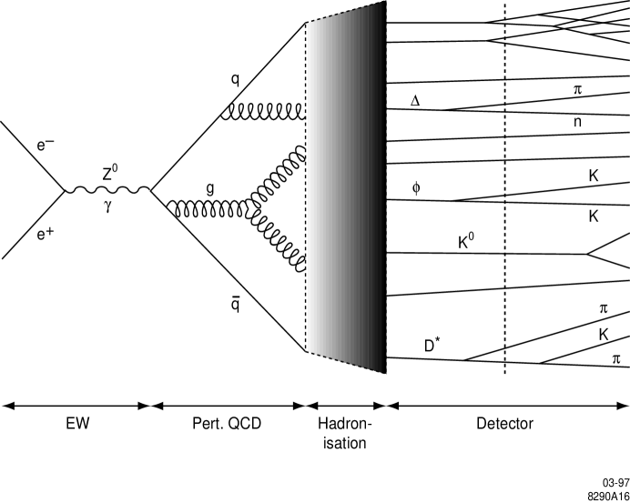
Figure 29: Schematic of hadron production in e⁺e^- annihilation.

4.4.2 Hadronisation and Monte Carlo Models

A schematic of hadron production in e⁺e^- annihilationis shown in Fig. 29. One may divide this process into several phases:

1. A hard electroweak process in which the primary quark and antiquark may be produced off mass-shell:

e⁺e^- $\rightarrow$q$\overline{\rm q}$

2. Perturbative QCD evolution of the primary q$\overline{\rm q}$via parton Bremsstrahlung:

q$\overline{\rm q}$ $\rightarrow$ several q, $\overline{\rm q}$, g

3. Hadronisation of partonic system:

(q, $\overline{\rm q}$, g)s  $\rightarrow$ primary resonances

4. Decays of primary resonances into ‘stable’ particles:

B, C, K${}^{0}_{s}$, $\phi$, $\Delta$, $\rho$ $\ldots$ $\rightarrow$$\pi^{\pm}$, K^±, p,$\overline{\rm p}$$\ldots$  (e^±, $\mu^{\pm}$, $\tau^{\pm}$, $\nu$)

Phases 1 and 2 are generally agreed to be calculable ‘respectably’ using perturbative techniques applied to the electroweak theory and QCD, respectively. Phases 3 and 4 are more problematic in that they are intrinsically non-perturbative processes that cannot in general be calculated from first principles. In the absence of non-perturbative calculations we are forced to rely on phenomenological models.

Since it is also necessary in phase 4 to simulate the interaction of particles with detectors, which can only be done in a deterministic fashion, Monte Carlo event generators have been developed for the complete simulation of hadronic event production in e⁺e^- annihilationand are now essential components of data analysis. I shall discuss only the two most widely used generators JETSET [59] and HERWIG [60]; other generators are described in [61], and will be discussed later by Buchanan [62]. I shall not discuss at all the GEANT program [63], which is widely used for the simulation of the geometry and material response of particle detectors. The philosophy here is to outline the main features of these generators in the context of their use as tools in understanding and correcting the data; no attempt will be made to justify these models on phenomenological grounds, and the outline will necessarily be brief.

Both JETSET and HERWIG implement electroweak matrix elements for the production of a primary q$\overline{\rm q}$, as well as a perturbative QCD ‘parton shower’ evolution of the system into a set of low-virtual-mass quarks and gluons. More formally, the latter is based on a probabilistic parton branching process that is derived from a leading + partial next-to-leading logarithmic resummation of the QCD matrix elements [64]. JETSET and HERWIG implement the parton branching process slightly differently, a discussion of which is beyond the scope of these lectures, but both generators have a parameter $\Lambda$ that characterises the scale of strong interactions, as well as a parameter $Q_{0}$ that characterises the minimum virtual-mass scale of the parton evolution.

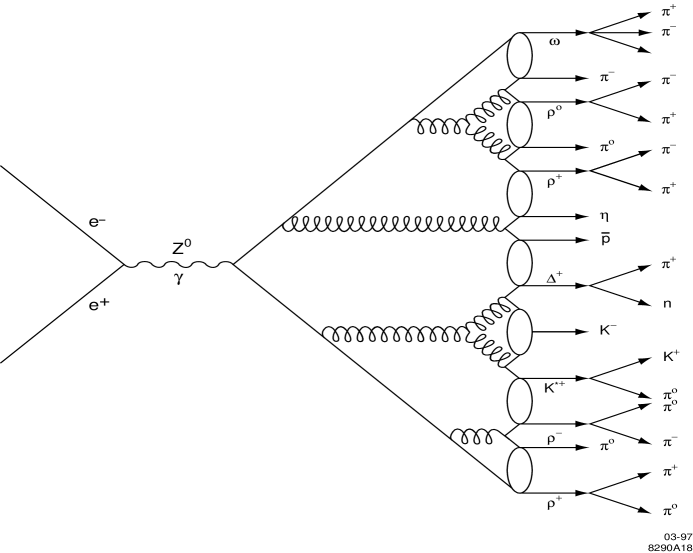
Figure 30: Schematic of hadronisation in HERWIG.

A schematic of the hadronisation process as implemented in HERWIG is shown in Fig. 30. At the termination of the parton shower pairs of partons are associateed into colourless clusters; these then undergo phase-space decay to produce stable pions, kaons and baryons. Clusters with mass larger than a parameter $M_{cl}$ are split into two before the phase-space decay. Additional parameters control the properties of heavy (B or C) hadron decay [60].

JETSET implements the ‘Lund string model’ of jet fragmentation [65], illustrated in Fig. 31. In this case the colour field between partons at the end of the parton shower is represented as a one-dimensional massless relativistic string. String pieces terminate at quarks and antiquarks, and gluons are represented by momentum-carrying ‘kinks’ in the string. The string is fragmented iteratively according to the recipe:

$$f(z)\quad\propto\quad\frac{1}{z}(1-z)^{a}{\rm exp}({-b\frac{m_{\perp}^{2}}{z}})$$ (39)

where $z$ is the fraction of the quantity $E+p_{\parallel}$ of a parent string piece taken by the daughter, $m_{\perp}$ = $\sqrt{p_{\perp}^{2}+m^{2}}$, ‘$\perp$’ and $`\parallel$’ refer to the string axis, and $a$ and $b$ are parameters. Momentum transverse to the string axis, $p_{\perp}$, is introduced in an ad hocfashion using a Gaussian probability distribution. A large number of additional parameters is used to fine-tune the relative production of particles such as strange, pseudoscalar, and vector mesons, as well as strange and non-strange, octet and decuplet baryons [59].

Figure 31: Schematic of hadronisation in JETSET.

4.4.3 Data Correction

For the $\alpha_{s}$analysis we wish to use these event generators to understand the effect of the hadronisation process on the hadronic momentum flow in events, and to correct for any bias, as well as to understand the influence of the response of the detector. One conventional approach involves using a sample of Monte Carlo events to calculate bin-by-bin correction factors, and then applying these to the measured distribution. For a distribution $D(X)$, the correction for detector effects is defined:

$$C_{DET}^{MC}(X)\quad=\quad{D_{HAD}^{MC}(X)\over D_{DET}^{MC}(X)},$$ (40)

where $HAD$ and $DET$ refer to the simulated distribution at the hadron-level and detector-level phases, respectively. The correction for hadronisation effects is analogously defined:

$$C_{HAD}^{MC}(X)\quad=\quad{D_{PART}^{MC}(X)\over D_{HAD}^{MC}(X)},$$ (41)

where $PART$ refers to the simulated distribution at the parton-level. The data distribution corrected back to the parton-level is given by:

$${D^{Data}}^{\prime}(X)\quad=\quad C_{HAD}^{MC}(X)\cdot C_{DET}^{MC}(X)\cdot D^{Data}(X),$$ (42)

and ${D^{Data}}^{\prime}(X)$ can be compared with perturbative QCD. More sophisticated correction procedures can also be defined; see eg. [66].

As with any correction procedure one must take care not to introduce bias from implicit model-dependence, and must estimate the systematic uncertainties involved. A prerequisite is that the simulation describe the distribution measured in the detector! The parameters of the detector simulation, as well as of the event generator itself, should then be varied, the stability of the correction factors examined, and systematic errors assigned accordingly. An example of a raw measured $D_{2}$ distribution from SLD [58], compared with simulations based on JETSET and HERWIG, is shown in Fig. 32. The corresponding corrected distribution, and the correction factors, are shown in Fig. 33.

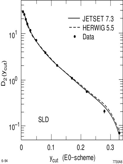
Figure 32: Measured $D_{2}$ distribution [58] compared with JETSET and HERWIG predictions.

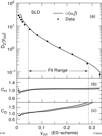
Figure 33: (a) Corrected $D_{2}$ distribution [58]; (b) hadronisation correction factor; (c) detector effects correction factor. In (a) the line shows a fit to O($\alpha_{s}^{2}$)QCD.

4.4.4 Comparison with Perturbative QCD

A fit of O($\alpha_{s}^{2}$)perturbative QCD to the $D_{2}$ distribution is shown in Fig. 33; it yields $\alpha_{s}(M_{Z}^{2})$= 0.1175 $\pm 0.0007$ (stat.) $\pm 0.0027$ (syst.) [58]. One can repeat this procedure for all 15 observables listed in Table 3 and derive in each case a fitted value of $\alpha_{s}(M_{Z}^{2})$; these are shown in Fig. 34a. The distressing result of this exercise is that the $\alpha_{s}(M_{Z}^{2})$values so determined are not internally consistent with one another! A measure of the scatter among the results is given by the r.m.s. deviation of $\pm 0.008$, which is much larger than the experimental error of $\pm 0.003$ on a typical observable. An exciting, though remote, possibility is that we have observed a spectacular breakdown of QCD! A more likely explanation is that some systematic effect that we have not yet considered is at work. In fact an implicit assumption was made in deriving the results shown in Fig. 34a that relates to the arcane issue of choosing the renormalisation scale in QCD.

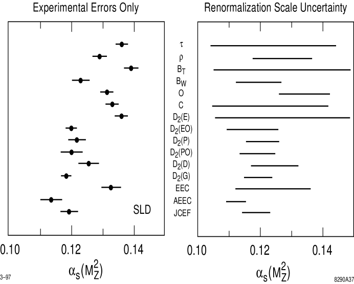
Figure 34: (a) Values of $\alpha_{s}(M_{Z}^{2})$determined [58] by fitting O($\alpha_{s}^{2}$)QCD predictions to 15 hadronic event shape observables using a fixed value of the renormalisation scale $\mu$ = $Q$; the results are clearly inconsistent within the experimental errors. (b) Renormalisation scale uncertainties.

4.4.5 Renormalisation Scale Uncertainty

For any observable, truncation of the QCD perturbation series at finite order causes a residual dependence on the (scheme-dependent) renormalisation scale $\mu$. This parameter is formally unphysical and should not enter at all into an exact infinite-order calculation, and its value is arbitrary. For the event shape observables an explicit $\mu$-dependence enters the next-to-leading coefficient:

$${1\over\sigma_{0}}{{\rm d}\sigma\over{\rm d}X}\;=\;A(X)\;\left({\alpha_{s}(\mu^{2})\over 2\pi}\right)\;+\;(\;B(X)\quad+\;A(X)2\pi b_{0}\;{\rm ln}\mu^{2}/Q^{2}\;)\left({\alpha_{s}(\mu^{2})\over 2\pi}\right)^{2}$$ (43)

so that a measurement of $\alpha_{s}$must be in the context of some chosen value of $\mu$. This is illustrated in Fig. 35, where the value of $\Lambda_{\overline{MS}}$from fits to $D_{2}$ is shown as a function of the choice of $\mu$; there is clearly a strong $\mu$-dependence. The top portion of Fig. 35 shows the corresponding $\chi^{2}_{dof}$ for each fit; amusingly the data show no preference for any particular value of $\mu$ provided it is larger than $\sqrt{0.001Q^{2}}$. A full discussion of the form of the $\mu$-dependence is beyond the scope of these lectures; see [67]. Figures of the $\mu$-dependence for the other observables can be found in [58].

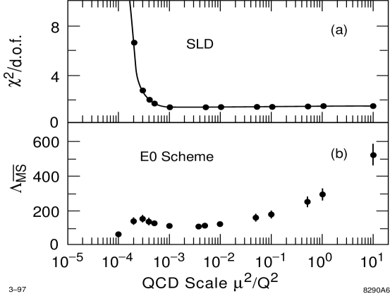
Figure 35: Dependence of (a) $\chi^{2}_{dof}$ and (b) $\Lambda_{\overline{MS}}$on the value of $\mu$ chosen in fits to the SLD $D_{2}$ distribution [54].

A consensus has arisen among experimentalists that the effect of missing higher-order terms can hence be estimated from the dependence of $\alpha_{s}(M_{Z}^{2})$on the value of $\mu$ assumed in fits of the calculations to the data, and a renormalisation scale uncertainty is often quoted. This procedure, well-motivated in that the $\mu$-dependence caused by the truncation of the perturbation series would be cancelled by addition of the higher-order terms, is, however, arbitrary, and is not equivalent to knowledge of the size of the a prioriunknown terms. In cases where scale uncertainties are considered this arbitrariness is manifested in the wide variation among the ranges and central values of $\mu$ chosen by different experimental groups, see eg.[68]; in other cases this source of uncertainty is not included in the errors. Different $\alpha_{s}(M_{Z}^{2})$results with similar experimental precision can hence be quoted with different total errors depending on the procedure adopted for assigning the theoretical uncertainties. The interpretation of the central values and errors on $\alpha_{s}(M_{Z}^{2})$measurements is hence not always straightforward. The SLD estimate of the renormalisation scale uncertainty for each observable is shown in Fig. 34b. It is apparent that the scale uncertainty is much larger than the experimental error, and that the $\alpha_{s}(M_{Z}^{2})$values are consistent within these uncertainties. Though this is comforting, in that it indicates that QCD is self-consistent, the necessary addition of large theoretical uncertainties to otherwise precise experimental measurements is frustrating, at least to experimentalists!

The best resolution of the scale ambiguity would be to reduce its effect by calculating observables to higher order in perturbation theory. Though this is in principle possible, the large number of Feynman diagrams involved renders the task difficult and unattractive. In e⁺e^- annihilationonly the $R$-related observables and the $\tau$ hadronic decay ratio $R_{\tau}$, have been calculated exactly up to O($\alpha_{s}^{3}$). For the hadronic event shape observables O($\alpha_{s}^{3}$)contributions have not yet been calculated completely. However, for six observables (indicated in Table 3) improved calculations can be formulated that incorporate the resummation [69] of leading and next-to-leading logarithmic terms matched to the O($\alpha_{s}^{2}$)results. The matched calculations are expected a priori both to describe the data in a larger region of phase space than the fixed-order results, and to yield a reduced dependence of $\alpha_{s}$on the renormalization scale. This is illustrated in Fig. 36 for the case of thrust ($\tau$). Though not well described by the O($\alpha_{s}^{2}$)calculation, the low-$\tau$ region is well reproduced when resummed contributions are included.

Application of other approaches to circumvent the scale ambiguity in $\alpha_{s}$ measurement, involving the use of ‘optimised’ perturbation theory’ [70] and Pad${\acute{\rm e}}$ Approximants [71], can be found in [68, 72] respectively.

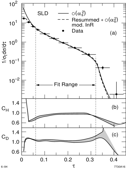
Figure 36: Illustration of the need for resummed contributions: the $\tau$ distribution measured by SLD [58]. At low $\tau$ the O($\alpha_{s}^{2}$)calculation is unable to describe the data unless resummed terms are considered.

4.4.6 Summary of $\alpha_{s}$Measurements

Hinchliffe has reviewed the various hadronic event shapes-based measurements from experiments performed in the c.m. energy range $10\leq Q\leq 91$ GeV, utilising both O($\alpha_{s}^{2}$)and resummed calculations, and quotes an average value of $\alpha_{s}(M_{Z}^{2})$= $0.122\pm 0.007$ [34], where the large error is dominated by the renormalisation scale uncertainty, which far exceeds the experimental error of about $\pm 0.002$. Schmelling has also compiled the measurements, including the recent results from the LEP-II run at $Q$ $\sim$ 133 GeV [73], and quotes a global average [74] $\alpha_{s}(M_{Z}^{2})$= $0.121\pm 0.005$, in agreement with [34], but assuming a more aggressive scale uncertainty.

4.5 Scaling Violations in Fragmentation Functions

Though distributions of final-state hadrons are not, in general, calculable in perturbative QCD, the $Q^{2}$-evolution of the scaled energy ($x_{p}=2E/Q$) distributions of hadrons, or ‘fragmentation functions’, can be calculated and used to determine $\alpha_{s}$. In addition to the usual renormalisation scale $\mu$, a factorisation scale $\mu_{F}$ must be defined that delineates the boundary between the calculable perturbative, and incalculable non-perturbative, domains. Additional complications arise from the changing composition of the underlying event flavour with $Q$ due to the different $Q$-dependence of the $\gamma$ and $Z^{0}$ exchange processes. Since B and C hadrons typically carry a large fraction of the beam momentum, and contribute a large multiplicity from their decays, it is necessary to consider the scaling violations separately in b, c, and light quark events, as well as in gluon jet fragmentation.

In an early analysis [75] the DELPHI Collaboration parametrised the fragmentation functions using the O($\alpha_{s}^{2}$)matrix elements and the string fragmentation model implemented in JETSET [59]. They fitted data in the range $14\leq Q\leq 91$ GeV to determine $\alpha_{s}(M_{Z}^{2})$= $0.118\pm 0.005$, where the error is dominated by varying $\mu$ in the range $0.1\leq\mu/Q\leq 1$. The ALEPH Collaboration used its $Z^{0}$ data to constrain flavour-dependent effects by tagging event samples enriched in light, c, and b quarks, as well as a sample of gluon jets [76]. The fragmentation functions for the different flavours and the gluon were parametrised at a reference energy, evolved with $Q$ according to the perturbative DGLAP formalism calculated at next-to-leading order [77], in conjunction with a parametrisation proportional to $1/Q$ to represent non-perturbative effects (Section 5), and fitted to data in the range $22\leq Q\leq 91$ GeV (Fig. 37). They derived $\alpha_{s}(M_{Z}^{2})$= $0.126\pm 0.007$ (exp.) $\pm 0.006$ (theor.), where the theoretical uncertainty is dominated by variation of the factorisation scale $\mu_{F}$ in the range $-1\leq{\rm ln}\mu_{F}^{2}/Q^{2}\leq 1$; variation of the renormalisation scale in the same range contributed only $\pm 0.002$. DELPHI has recently reported a similar analysis [78] yielding $\alpha_{s}(M_{Z}^{2})$= $0.121^{+0.006}_{-0.007}$ (exp.) $\pm 0.010$ (theor.). Curiously, although a similar range as ALEPH, $0.3\leq\mu/Q\leq 3$, was used to examine variation of the renormalisation and factorisation scales, here the renormalisation scale dominates the theoretical uncertainty, with a contribution of $\pm 0.009$, in contrast to $\pm 0.002$ from factorisation. Combining the ALEPH and later DELPHI results, assuming uncorrelated experimental errors, yields [32]:

$$\alpha_{s}(M_{Z}^{2})\quad=\quad 0.124\pm 0.005({\rm exp.})\pm 0.010({\rm theor.})$$ (44)

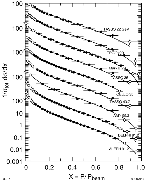
Figure 37: Illustration of scaling violations in e⁺e^-fragmentation functions.

4.6 Comparison with Other Measurements of $\alpha_{s}(M_{Z}^{2})$

A summary of world $\alpha_{s}$measurements, all evolved to $Q$ = $M_{Z}$, is shown in Fig. 38 [32]. These are drawn from lepton-hadron scattering, hadron-hadron collisions, heavy quarkonia decays and lattice gauge theory, as well as e⁺e^- annihilation. In addition to being relatively precise, the e⁺e^-results have the invaluable feature that they bracket the $Q$-range of the experiments, from around 1 GeV for $\tau$ decays to around 100 GeV for $Z^{0}$ production, providing the largest lever-arm for tests of consistency of $\alpha_{s}(M_{Z}^{2})$measured at different energy scales. It is clear that, within the uncertainties, all results are consistent with one another.

Figure 38: Summary of world $\alpha_{s}(M_{Z}^{2})$measurements [32]. The results are ordered vertically in terms of the hard scale $Q$ of the experiment.

Taking an average over all 17 measurements assuming they are independent, by weighting each by its total error, yields $\alpha_{s}(M_{Z}^{2})$= 0.118 with a $\chi^{2}$ of 6.4; the low $\chi^{2}$ value reflects the fact that most of the measurements are theoretical-systematics-limited. Taking an unweighted average, which in some sense corresponds to the assumption that all 17 measurements are completely correlated, yields the same result. The r.m.s. deviation of the 17 measurements w.r.t. the average value characterises the dispersion, and is $\pm 0.005$. In a quantitative sense, therefore, QCD has been tested to a level of about 5%.

If further progress is to be made in testing QCD, future measurements of $\alpha_{s}(M_{Z}^{2})$should aim for substantially improved precision. The prospects for achieving 1%-level measurements are discussed in detail elsewhere [79]. Lattice QCD determinations may reach this precision within the next few years. A precise $\alpha_{s}(M_{Z}^{2})$measurement has yet to emerge from the TeVatron, but feasibility studies are in progress and appear promising. Deep-inelastic scattering and e⁺e^- annihilationwill probably require higher-energy facilities, as well as significant theoretical effort with regard to O($\alpha_{s}^{3}$)perturbative contributions. An $\alpha_{s}(M_{Z}^{2})$ measurement at a high-energy e⁺e^-collider will be discussed in Section 6.2.

5. Towards a Theory of Hadronisation

We expect that the strong coupling becomes large in long-distance (low-$Q$) q$-$q interactions such that finite-order perturbation theory is no longer valid. Lattice gauge theory [80] is the only practical non-perturbative calculational tool available today. It is presently limited in applicability to static properties of hadrons, such as masses and decay constants, although in principle it might eventually be applied to the dynamical process of hadronisation.

From the operator product expansion (OPE) one expects (see eg. [81]) that the expectation value of an observable $O$ may be written:

$$<O>\quad=\quad\Sigma{\;a_{i}\left({\alpha_{s}\over\pi}\right)^{i}}\quad+\quad\Sigma{\;b_{j}\over Q^{j}}$$ (45)

During the past 15 years much theoretical effort has been focussed on the perturbative component represented by the first term in this equation. More recently attention has turned to the ‘power corrections’ represented by the second term, whose origin is intrinsically non-perturbative. In particular, attempts have been made to evaluate power corrections for e⁺e^-observables. An illustration of the potential of such an approach is provided by Fig. 39 [82]. The ad hocaddition of a $1/Q$ term to the O($\alpha_{s}^{2}$)QCD prediction describes the energy-dependence of $<1-T>$ remarkably well. It will be seen in Section 6.2 that the inverse power-law behaviour of hadronisation effects has important consequences for a precise $\alpha_{s}$measurement at a high energy e⁺e^-collider. The explicit calculation of leading power corrections [81] hence represents our first tentative step towards a consistent theoretical treatment of hadronisation.

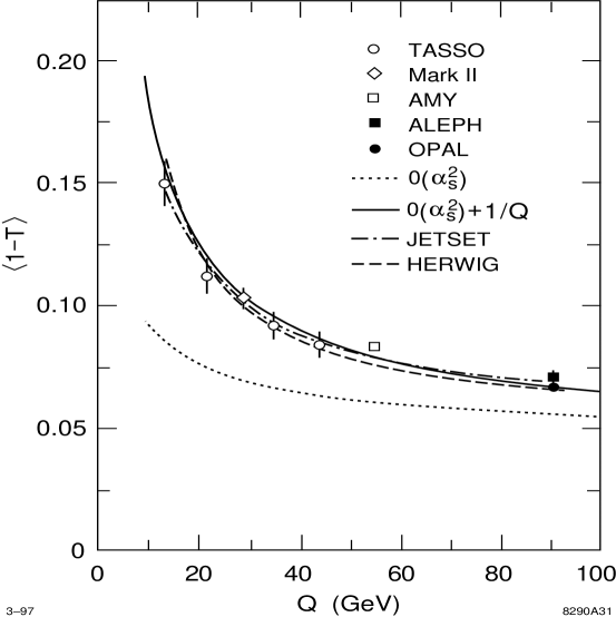
Figure 39: Energy-dependence of the mean value of $1-T$. The ad hocaddition of a $1/Q$ term to the O($\alpha_{s}^{2}$)QCD prediction describes the data [82].

6. QCD at a High Energy e⁺e^-Collider

6.1 Introduction

Since QCD is our theory of strong interactions it would be irresponsible not to test it at the highest energy scales available in different hard scattering processes. For this reason testing QCD at a 0.5–1.5 TeV e⁺e^-collider (‘XLC’) is mandatory. For a detailed discussion see [83].

Precise determination of the strong coupling $\alpha_{s}$is key to a better understanding of high energy physics. The current precision of $\alpha_{s}(M_{Z}^{2})$measurements, limited to about 5% (Section 4.6), results in the dominant uncertainty on our prediction of the energy scale at which grand unification of the strong, weak and electromagnetic forces takes place. An $\alpha_{s}(M_{Z}^{2})$measurement of 1% precision may be possible at a high energy e⁺e^-collider. Such a measurement would also allow improved determination of the mass and width of the top quark from the threshold behaviour of the ${\rm t}\bar{\rm t}$ cross-section. Measurements of hadronic event properties at high energies, combined with existing lower energy data, would allow one to test further the gauge structure of QCD by searching for anomalous ‘running’ of observables, such as the rate of production of events containing three jets, and to set limits on models which predict such effects, for example those involving light gluinos which are difficult to exclude by other means.

Gluon radiation in ${\rm t}\bar{\rm t}$ events is expected to be strongly regulated by the large mass and width of the top quark; t$\overline{\rm t}$gevents will hence provide an exciting new domain for QCD studies. As a corollary, measurements of gluon radiation patterns in t$\overline{\rm t}$gevents may provide valuable additional constraints on the top quark decay width. Furthermore, searches could be made for anomalous chromo-electric and chromo-magnetic moments of quarks [84], which effectively modify the rate and pattern of gluon radiation, and for which the phase space increases as the c.m. energy is raised. Finally, polarised electron beams will be exploited at high energy e⁺e^-colliders and will allow tests of symmetries using multi-jet final states [85].

6.2 Is a 1%–level Measurement of $\alpha_{s}(M_{Z}^{2})$Possible?

It is interesting to consider whether a measurement of $\alpha_{s}(M_{Z}^{2})$at the 1%–level of precision is possible at the XLC. Consider the SLD $\alpha_{s}(M_{Z}^{2})$measurement, discussed in Section 4.4, based on 15 hadronic event shape observables measured with a data sample comprising approximately 50,000 hadronic events [58]:

$$\alpha_{s}(M_{Z}^{2})\quad=\quad 0.1200\pm 0.0025\;{\rm(exp.)}\pm 0.0078\;{\rm(theor.)}$$ (46)

where the experimental error is composed of statistical and systematic components of about $\pm 0.001$ and $\pm 0.002$ respectively, and the theoretical uncertainty has components of $\pm 0.003$ and $\pm 0.007$ arising from hadronisation and missing higher order terms, respectively. Now consider ‘scaling’ this result to estimate the precision of a similar measurement at $Q$ = 500 GeV.

$\bullet$ Statistical error: At design luminosity the 500 GeV XLC would deliver roughly 100,000 q$\overline{\rm q}$  (q=u,d,s,c,b) events per year (Section 6.4), implying that a statistical error on $\alpha_{s}(M_{Z}^{2})$well below $\pm$ 0.001 could be obtained.

$\bullet$ Systematic error: This results primarily from the uncertainty in modelling the jet resolution of the detector. The situation may be improved at the XLC by a combination of building better detectors and benefitting from improved calorimeter energy resolution for higher energy jets. It is not unreasonable to suppose that the current systematic error of roughly $\pm 0.002$ could be reduced by a factor of two.

$\bullet$ Hadronisation uncertainty: From the discussion in Section 5 it can be seen that non-perturbative corrections to jet final states in e⁺e^- annihilationcan be parametrised in terms of inverse powers of the hard scale $Q$. At leading order, perturbative evolution is proportional to ${1/{\rm ln}Q}$. Hence for a generic observable $X$ the ratio of non-perturbative to perturbative QCD contributions is dominated by a term of the form:

$${\delta X^{\rm non-pert}\over X^{\rm pert}}\quad\sim\quad{{\rm ln}Q\over Q}.$$ (47)

Increasing $Q$ from 91 GeV to 500 GeV causes this ratio to decrease by a factor of 5, implying that hadronisation corrections in the ‘3-jet region’ of observables should be of order 2% at XLC. The conclusion of this analysis is reinforced by explicit simulation of hadronisation effects, illustrated in Fig. 40 [86] for thrust. Assuming that these corrections can be estimated to better than $\pm 50$%, the hadronisation uncertainty should contribute less than 1% to the error on $\alpha_{s}(M_{Z}^{2})$.

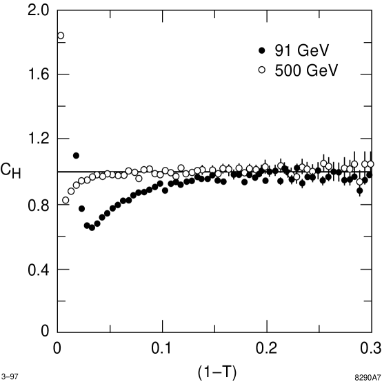
Figure 40: Estimate of the hadronisation correction factor (Section 4.4.2) for thrust at $Q$ = 91 GeV and 500 GeV [86]. At 500 GeV the factor barely deviates from unity for most of the kinematic range.

$\bullet$ Uncertainty due to missing higher orders: Currently perturbative QCD calculations of hadronic event shapes are available complete up to O($\alpha_{s}^{2}$). Since the data contain knowledge of all orders one must estimate the possible bias inherent in measuring $\alpha_{s}(M_{Z}^{2})$using the truncated QCD series (Section 4.4.5). Since the missing perturbative terms are O($\alpha_{s}^{3}$), and since at $Q$ = 500 GeV $\alpha_{s}$is expected to be about 25% smaller than its value at the $Z^{0}$, one naively expects the uncalculated terms to be almost a factor of two smaller at the higher energy, leading to an estimated uncertainty of $\pm 0.004$ on $\alpha_{s}$(500 GeV). However, translating to the yardstick $\alpha_{s}(M_{Z}^{2})$yields an uncertainty of $\pm 0.006$, only slightly reduced compared with the current uncertainty.

From this simple analysis it seems reasonable to conclude that achievement of the luminosity necessary for ‘discovery potential’ at the XLC will result in a q$\overline{\rm q}$event sample of sufficient size to measure $\alpha_{s}(M_{Z}^{2})$with a statistical uncertainty of better than 1%. Construction of detectors superior in performance to those in operation today at SLC and LEP may be necessary in order to reduce systematic errors to the 1% level. Hadronisation effects should be significantly smaller, implying a sub–1% uncertainty. However, unless O($\alpha_{s}^{3}$)contributions are calculated, $\alpha_{s}(M_{Z}^{2})$measurements at 500 GeV will be limited by theoretical uncertainties to a precision of $\pm 0.006$, only marginally better than that achieved at present.

6.3 Top Quark Mass Determination and $\alpha_{s}$

It is clear that the value of $\alpha_{s}$controls the shape of the strong potential that binds quarkonia resonances. In the case of ${\rm t}\bar{\rm t}$ production near threshold, the large top mass $m_{t}$, and hence large decay width $\Gamma$, ensure that the top quarks decay in a time comparable with the classical period of rotation of the bound system, making the toponium resonance a very short-lived phenomenon, and washing out most of the resonant structure in the cross-section. The shape of the ${\rm t}\bar{\rm t}$ cross-section near threshold hence depends strongly not only on the top mass, but also on $\alpha_{s}$.

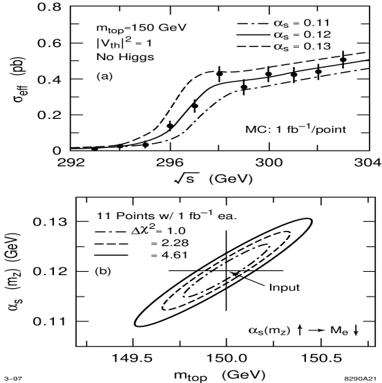
Figure 41: Simulation of a simultaneous measurement of $\alpha_{s}(M_{Z}^{2})$and $m_{t}$ at a high-energy e⁺e^-collider [87]: (a) ${\rm t}\bar{\rm t}$ production cross section; (b) correlation between fitted values.

Fits to simulations of measurements of this cross-section have shown [87] that the top mass so determined is strongly correlated with the assumed value of $\alpha_{s}(M_{Z}^{2})$. This is illustrated in Fig. 41. The European Top Quark Working Group has updated these simulations for the latest measured values of the top mass and has shown [88] that a simultaneous determination of $m_{t}$ and $\alpha_{s}(M_{Z}^{2})$by fitting to the threshold cross-section measured with one design-year of luminosity yields statistical precisions of $\pm$250 MeV/$c^{2}$ and $\pm 0.006$ on $m_{t}$ and $\alpha_{s}(M_{Z}^{2})$, respectively. Fixing $\alpha_{s}(M_{Z}^{2})$to 0.120 reduces the error on $m_{t}$ by a factor of 2. Since this technique would yield a measurement of $\alpha_{s}(M_{Z}^{2})$no more precise than those made today, and since systematic uncertainties may be large and have not yet been considered, a more sensible strategy would be to measure $\alpha_{s}(M_{Z}^{2})$as precisely as possible, as described in the previous section, and to use this value to allow better determination of the top quark parameters.

6.4 Energy Evolution Studies

The non-Abelian gauge structure of QCD implies that as the hard scattering scale $Q$ increases, the strong coupling decreases roughly as 1/ln$Q$. Existing hadronic final states data from e⁺e^- annihilationat the PETRA, PEP, TRISTAN, SLC and LEP colliders span the range $14\leq Q\leq 170$ GeV, although hadronisation uncertainties are large on the data below 25 GeV. A 1.5 TeV e⁺e^-collider would increase the lever-arm in 1/ln$Q$ by almost a factor of two, hence allowing detailed study of the energy evolution of QCD observables that are proportional to $\alpha_{s}$, such as the rate of production of final states containing three hadronic jets, $R_{3}$. This would provide not only a test of the fundamental structure of SU(3) QCD, but also a search-ground for new physics that might produce ‘anomalous’ running.

One such possibility is the existence of a light, electrically neutral, coloured fermion that couples to gluons, often called a ‘light gluino’ and denoted by $\tilde{g}$ . The existence of such a particle would manifest itself via a modification of gluon vacuum polarisation contributions involving fermion loops, effectively increasing the number of light fermions entering into the QCD $\beta$-function. At one-loop level the effective number of flavours would change from $N_{F}$ to $N_{F}+3N_{\tilde{g}}$, where $N_{\tilde{g}}$ is the number of families of light gluinos, causing a decrease in the running of $\alpha_{s}$as a function of $Q$. The existence of a light gluino of mass between 2 and 5 GeV/$c^{2}$ has not been excluded by searches with current data [86]. A simulated measurement of $R_{3}$ at $Q$ = 500 GeV, corresponding to one design-luminosity-year, is shown in Fig. 42 [86], together with existing measurements, plotted as a function of 1/ln$Q$. The presence of one family of light gluinos of mass 2 GeV/$c^{2}$ would cause an increase in the predicted value of $R_{3}$ at 500 GeV by 10%. A 1%-level measurement of $R_{3}$, as discussed in the previous section, would allow this difference to be measured with a significance of many standard deviations.

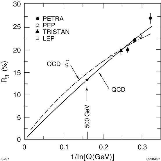
Figure 42: Energy-evolution of the 3-jet rate $R_{3}$ [86]. For illustration an O($\alpha_{s}^{2}$)QCD fit, as well as a fit allowing the possibility of one family of light gluinos, is shown. The simulated data point at $Q$ = 500 GeV would add considerable lever-arm.

It should be noted, however, that data from a number of experiments at different e⁺e^-colliders contribute to Fig. 42. Some of these data were recorded more than 10 years ago, were treated differently by the various experimental groups, and have relatively large systematic errors that are at least partly uncorrelated from point to point. Furthermore, the sophistication and performance of particle detectors constructed in the last decade has improved significantly, and it is reasonable to assume that future detectors will be even better. In addition, our understanding of the modelling of hadronisation effects and theoretical uncertainties has improved enormously as a result of studies at the $Z^{0}$. Therefore, the precision of searches for anomalous running of QCD observables at XLC would be improved significantly if new data were taken at the lower c.m. energies with the same detector and analysis procedures.

In fact, if the luminosity of the 500 GeV XLC could be preserved at lower c.m. energies, very large data samples would be recorded. Table 4 [86] shows the number of q$\overline{\rm q}$events delivered per day at various c.m. energies by the XLC operating at the design luminosity of $5\times 10^{33}$ cm${}^{-2}s^{-1}$. At each energy more luminosity would be delivered per day than was recorded in total by the original dedicated colliders! This argument is of course naive, in that a collider designed to operate at a luminosity of $5\times 10^{33}$ cm${}^{-2}s^{-1}$ at 500 GeV would not automatically be operable at the same luminosity at energies a factor of 5 or 10 lower; such capability would have to be designed from the outset. Furthermore, the requirements on the triggering and data processing capabilities of the detector are extreme by the standards of e⁺e^- annihilation, and this would also have to be designed from the start. Nevertheless, the prospect of running the XLC at the $Z^{0}$ resonance, or at even lower energies, for QCD studies, not to mention high-statistics electroweak physics measurements, is very attractive.

c.m. energy $Q$ (GeV)	q$\overline{\rm q}$events/day
500	1750
91	20,000,000
60	75,000
35	150,000

Table 4: Number of q$\overline{\rm q}$events per day delivered by an e⁺e^-collider operating at a luminosity of $5\times 10^{33}$ cm${}^{-2}s^{-1}$.

6.5 Gluon Radiation in ${\rm t}\bar{\rm t}$ Events

The large mass and decay width of the top quark serve to make the study of gluon radiation in ${\rm t}\bar{\rm t}$ events a new arena for testing QCD. The large mass acts as a cutoff for collinear gluon radiation, and the large decay width acts as a cutoff for soft gluon radiation, allowing reliable perturbative QCD calculations to be performed; these effects are of course correlated. The latter case is particularly interesting. If the top width were infinite, top quarks would decay immediately to bottom quarks, and any gluons would be radiated from the secondary b’s. If the top width were zero, top quarks would live forever and all radiation would be from the primary t’s. In the case of a large but finite width, expected to be around 2 GeV for a top mass of 180 GeV/$c^{2}$, gluon radiation in ${\rm t}\bar{\rm t}$ events will be a coherent sum of contributions from these two limiting cases, with a degree of coherence regulated by the top width itself.

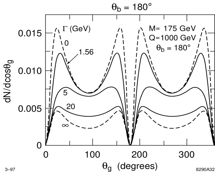
Figure 43: Angular distribution of 5 GeV gluons w.r.t. ${\rm t}\bar{\rm t}$ axis, at $Q$ = 1 TeV, illustrating the dependence on the top width $\Gamma$ [89].

A theoretical study of ${\rm t}\bar{\rm t}$ production above threshold, assuming $m_{t}$ = 175 GeV/$c^{2}$ at $Q$ = 1 TeV, is illustrated in Fig. 43 [89]. This shows the angular distribution of 5 GeV gluons w.r.t. the ${\rm t}\bar{\rm t}$ axis for the kinematic configuration in which the decay b-quark travels backwards w.r.t. the t flight direction. The dependence of the radiation pattern on the top decay width is strong. Similar effects are predicted in the spectrum of gluon radiation in ${\rm t}\bar{\rm t}$ events around threshold [90]. Measurement of such effects would yield not only a dramatic demonstration of quantum interference in strong interactions, but might also provide an essential cross-check on the value of the top quark decay width, which may prove difficult to disentangle from measurements of the ${\rm t}\bar{\rm t}$ threshold cross-section and top momentum distributions, which also depend on $\alpha_{s}$and $m_{t}$ (section 6.3), as well as on the beam energy distribution.

7. Concluding Remarks

We have seen that e⁺e^-annihilation is an ideal laboratory for precise studies of QCD. One observes jets indicating the primary production of quarks and gluons, and one can measure precisely the quark and gluon spins. Multijet events allow the very gauge structure of QCD to be tested via measurement of the Casimir factors $N_{C}$, $T_{F}$, and $C_{F}$, leading us to the conclusion that QCD is the theory of strong interactions. One can then measure the single parameter of QCD, the coupling $\alpha_{s}$, from inclusive observables such as $R$, or equivalently the $Z^{0}$ lineshape parameters, and from hadronic $\tau$ decays, as well as from event shape measures and scaling violations in inclusive single-particle fragmentation functions. These $\alpha_{s}(M_{Z}^{2})$measurements are internally consistent, and agree with results from lepton-nucleon scattering, hadron-hadron collisions, and lattice gauge theory determined across a wide range of energy scales.

There was no time to cover many interesting topics, including: differences between quark and gluon jets, tests of the flavour-independence of strong interactions, polarisation phenomena, particle multiplicities and correlations, production of B and C mesons and baryons, and production of identified hadrons such as $\pi^{\pm}$, K${}^{0}_{s}$, K^±, p/$\overline{\rm p}$, $\Lambda$, $\phi$, K^∗ etc.Some of these topics are discussed in other contributions to these proceedings [62, 91].

Looking towards the future, tests of QCD will provide an important component of the physics programme at a future high energy e⁺e^-collider operating in the c.m. energy range $0.5\leq Q\leq 1.5$ TeV. Measurement of $\alpha_{s}(M_{Z}^{2})$at the 1% level of precision appears feasible experimentally, but will require considerable theoretical effort to calculate O($\alpha_{s}^{3}$)contributions in QCD perturbation theory. A search for anomalous running of $\alpha_{s}$($Q^{2}$), by operating the collider at different c.m. energies, is an attractive prospect. Quantum coherence is expected to give rise to interesting gluon radiation patterns in ${\rm t}\bar{\rm t}$ events, which could be used to constrain the top quark decay width, and measurement of the gluon radiation spectrum would also constrain anomalous top quark chromomagnetic couplings.

More immediately, the next generation of low energy e⁺e^-colliders, known as B factories, also has the potential to make a precise $\alpha_{s}$measurement from the $R$-ratio at $Q$ $\approx$ 10 GeV, as well as from hadronic $\tau$ decays. Even more precise tests of QCD in e⁺e^- annihilationwill hence continue to enhance our confidence in the theory, and may even yield surprises$\ldots$

Acknowledgements

I am grateful for the support of my colleagues in the SLD Collaboration and the SLAC Theory Group. I thank Lance Dixon and David Muller for careful reading of this manuscript.

References

- [1]
- [2] M. Albrow, ‘QCD studies in hadron-hadron collisions’; these proceedings.
- [3] W. Smith, ‘QCD studies in lepton-hadron collisions’; these proceedings.
-
[4]
H. Fritzsch, M. Gell-Mann and H. Leutwyler, Phys. Lett. 47B (1973) 365;
D.J. Gross and F. Wilczek, Phys. Rev. Lett. 30 (1973) 1343;
H.D. Politzer, Phys. Rev. Lett. 30 (1973) 1346;
S. Weinberg, Phys. Rev. Lett. 31 (1973) 494. - [5] M. Gell-Mann, Phys. Rev. 125 (1962) 1067.
- [6] G. Kramer, Springer Tracts in Modern Physics, Vol. 102 (1984).
- [7] See eg., M. Gell-Mann, Y. Ne’eman, The Eightfold Way, Benjamin, New York (1972).
- [8] Mark I Collab., G. Hanson et al., Phys. Rev. Lett.35 (1975) 1609.
- [9] J.D. Bjorken, S.J. Brodsky, Phys. Rev.D1 (1970) 1416.
- [10] Mark I Collab., R.F. Schwitters et al., Phys. Rev. Lett.35 (1975) 1320.
- [11] See eg., V. Barger, R.J.N. Phillips, Frontiers in Physics, Vol. 71, ‘Collider Physics’, Addison-Wesley (1987).
- [12] TASSO Collab., M. Althoff et al., Z. Phys.C22 (1984) 307.
-
[13]
S. Brandt et al., Phys. Lett. 12 (1964) 57.
E. Farhi, Phys. Rev. Lett. 39 (1977) 1587. - [14] R. Marshall, Z. Phys.C43 (1989) 595.
-
[15]
TASSO Collab., R. Brandelik et al., Phys. Lett. 86B
(1979) 243.
Mark J Collab., D.P. Barber et al., Phys. Rev. Lett. 43 (1979) 830.
PLUTO Collab., Ch. Berger et al., Phys. Lett. 86B (1979) 418.
JADE Collab., W. Bartel et al., Phys. Lett. 91B (1980) 142. - [16] J. Ellis, M.K. Gaillard, G.G. Ross, Nucl. Phys. B111 (1976) 253.
- [17] S.L. Wu, Phys. Rep. 107 (1984) 59.
- [18] J. Ellis, I. Karliner, Nucl. Phys. B148 (1979) 141.
- [19] TASSO Collab., M. Althoff et al., Z. Phys.C22 (1984) 307.
-
[20]
P. Hoyer, P. Osland, H.G. Sander, T.F. Walsh and P.M. Zerwas,
Nucl. Phys. B161 (1979) 349;
E. Laermann, K.H. Streng and P.M. Zerwas, Z. Phys. C3 (1980) 289; erratum ibid C52 (1991) 352. - [21] T.G. Rizzo, private communications.
- [22] SLD Collab., K. Abe et al., Phys. Rev.D55 (1997) 2533.
- [23] TASSO Collab., W. Braunschweig et al., Z. Phys. C47 (1990) 181.
- [24] L3 Collab., B. Adeva et al., Phy. Lett. B263 (1991) 551.
- [25] DELPHI Collab., P. Abreu et al., Phys. Lett. B274 (1992) 498.
- [26] O. Nachtmann, A. Reiter, Z. Phys.C16 (1982) 45.
- [27] M. Bengtsson, P.M. Zerwas, Phys. Lett.B208 (1988) 306.
- [28] L3 Collab., B. Adeva et al., Phys. Lett.B248 (1990) 227.
- [29] OPAL Collab., R. Akers et al., Z. Phys.C65 (1995) 367.
- [30] OPAL Collab., OPAL Physics Note PN-188 (July 1995).
- [31] G.L. Kane et al., Phys. Lett.B354 (1995) 350.
- [32] P.N. Burrows, SLAC-PUB-7293 (1996); to appear in Proc. 3rd International Symposium on Radiative Corrections, August 1-5 1996, Cracow, Poland.
- [33] W.A. Bardeen, A.J. Buras, D.W. Duke, T. Muta, Phys. Rev.18 (1978) 3998; D.W. Duke, Rev. Mod. Phys.52 (1980) 199.
- [34] R.M. Barnett et al., Phys. Rev.D54 (1996) 77.
- [35] R.M. Barnett et al., Phys. Rev.D54 (1996) 19.
-
[36]
S.G. Gorishny, A. Kataev, S.A. Larin, Phys. Lett.B259 (1991) 144;
L.R. Surguladze, M.A. Samuel, Phys. Rev. Lett.66 (1991) 560. - [37] K.H. Chetyrkin, J.H. Kühn, A. Kwiatkowski, Berkeley preprint LBL 36678-Rev (1996); subm. to Phys. Rep.
- [38] A. Blondel, ‘Experimental status of electroweak interactions’, to appear in Proc. 28th International Conference on High Energy Physics, 25-31 August 1996, Warsaw, Poland.
- [39] P.B. Renton, Proc. 17th International Symposium on Lepton-Photon Interactions, 10-15 August 1995, Beijing, China, p. 35.
- [40] D. Schaile, Proc. XXVII International Conference on High Energy Physics, July 20-27 1994, Glasgow, Scotland, IoP Publishing, Eds. P.J. Bussey, I.G. Knowles, p. 27.
- [41] See eg.M. Shifman, Mod. Phys. Lett. A10 No. 7 (1995) 605.
- [42] J. Chyla, A.L. Kataev, Reports of the Working Group on Precision Calculations for the Z Resonance, eds. D. Bardin, W. Hollik, G. Passarino, CERN 95-03 (1995) 313.
- [43] F. Le Diberder, A. Pich, Phys. Lett.B289 (1992) 165.
- [44] E. Braaten, S. Narison, A. Pich, Nucl. Phys.B373 (1992) 581; F. Le Diberder, A. Pich, Phys. Lett.B286 (1992) 147.
- [45] M. Neubert, Nucl. Phys.B463 (1996) 511.
- [46] L. Duflot (ALEPH Collab.), Nucl. Phys. B (Proc. Supp.) 39B (1995) 322.
- [47] OPAL Collab., R. Akers et al., Z. Phys.C66 (1995) 543.
- [48] CLEO Collab., T. Coan et al., Phys. Lett.B356 (1995) 580.
- [49] G. Altarelli, P. Nason, G. Ridolfi, Z. Phys.C68 (1995) 257.
- [50] R.K. Ellis, D.A. Ross, A.E. Terrano, Phys. Rev. Lett. 45 (1980) 1226; Nucl. Phys. B178 (1981) 421.
- [51] G. Kramer, B. Lampe, Z. Phys. C39 (1988) 101; Fortschr. Phys. 37 (1989) 161.
- [52] Z. Kunszt et al., CERN 89–08 Vol I, (1989) p. 373.
- [53] JADE Collab., W. Bartel et al., Z. Phys.C33 (1996) 23.
- [54] SLD Collab., K. Abe et al., Phys. Rev. Lett. 71 (1993) 2528.
- [55] S. Bethke et al., Nucl. Phys.B370 (1992) 310.
- [56] See eg., D. Soper, ‘Basics of QCD perturbation theory’; these proceedings.
- [57] MARK-J Collab., D. P. Barber et al., Phys. Rev. Lett. 43 (1979) 830; Phys. Lett. B89 (1979) 139.
- [58] SLD Collab., K. Abe et al., Phys. Rev.D51 (1995) 962.
- [59] T. Sjöstrand, CERN–TH–7112/93 (1993).
- [60] G. Marchesini et al., Comp. Phys. Comm. 67 (1992) 465.
- [61] I. Knowles et al., ‘QCD Event Generators’, hep-ph/9601212 (1996).
- [62] C.D. Buchanan, ‘New accurate ideas on flavor production in hadronization and their connections to QCD’; these proceedings.
- [63] R. Brun et al., CERN-DD/EE/84-1 (1989).
- [64] G. Marchesini, B.R. Webber, Nucl. Phys.B238 (1984) 1.
- [65] B. Andersson, et al., Phys. Rep. 97 (1983) 33.
- [66] V. Blobel, Proceedings of 8th CERN School of Computing, Aiguablava, Spain, September 9–22, 1984, CERN 85–09 (1985).
- [67] P.N. Burrows, H. Masuda, Z. Phys.C63 (1994) 235.
- [68] P.N. Burrows et al., Phys. Lett.B382 (1996) 157.
- [69] S. Catani, G. Turnock, B.R. Webber, and L. Trentadue, Phys. Lett. B263 (1991) 491.
-
[70]
P.M. Stevenson, Phys. Rev.D23 (1981) 2916;
G. Grunberg, Phys. Rev.D29 (1984) 2315;
S.J. Brodsky, G.P. Lepage, P.B. Mackenzie, Phys. Rev.D28 (1983) 228. - [71] See eg.G.A. Baker Jr., ‘Essentials of PadApproximants’, Academic Press, 1975.
- [72] P.N. Burrows et al., SLAC-PUB-7222 (1996); to appear in Phys. Lett.B.
- [73] D. Duchesneau, ‘QCD Results from LEP above and below the Peak’, to appear in Proc. 28th International Conference on High Energy Physics, Warsaw, Poland, 25-31 July 1996.
- [74] M. Schmelling, ‘Status of the Strong Coupling Constant’, to appear in Proc. 28th International Conference on High Energy Physics, Warsaw, Poland, 25-31 July 1996.
- [75] DELPHI Collab., P. Abreu et al., Phys. Lett.B311 (1993) 408.
- [76] ALEPH Collab., D. Buskulic et al., Phys. Lett.B357 (1995) 487.
- [77] G. Gurci, W. Furmanski, R. Petronzio, Nucl. Phys.B175 (1980) 27.
- [78] DELPHI Collab., W. de Boer et al., paper contributed to 28th International Conference on High Energy Physics, Warsaw, Poland, 25-31 July 1996, pa01-022.
- [79] P. Burrows et al., ‘Prospects for the precision measurement of ’, SLAC-PUB-7371 (1996); to appear in Proc. Workshop on Future Directions in High Energy Physics, June 25 - July 12 1996, Snowmass, Co, USA.
- [80] See eg., T. DeGrand, ‘Lattice gauge theory for QCD’; these proceedings.
- [81] M. Beneke, SLAC-PUB-7277 (1996); to appear in Proc. 28th International Conference on High Energy Physics, 25-31 August 1996, Warsaw, Poland;
- [82] B.R. Webber, Cavendish-HEP-94/17 (1994).
- [83] P.N. Burrows, Proc. Workshop on Physics and Experiments with Linear Colliders, September 8-12 1995, Morioka-Appi, Iwate, Japan, Ed. A. Miyamoto et al., World Scientific 1996, p. 179.
- [84] T.G. Rizzo, Phys. Rev. D50 (1994) 4478.
-
[85]
A. Brandenburg, L. Dixon, and Y. Shadmi, Phys. Rev.D53 (1996) 1264.
SLD Collaboration, K. Abe et al., Phys. Rev. Lett. 74 (1995) 4173. - [86] S. Bethke, Proc. Workshop on Physics and Experiments with Linear e+e- Colliders, April 1993, Waikoloa, Hawaii, Ed. F.A. Harris et al., World Scientific 1993, p. 687.
- [87] JLC Group, S. Matsumoto et al., KEK Report 92-16 (1992) p. 53.
- [88] P. Comas et al., Proc. Workshop on Physics and Experiments with Linear Colliders, September 8-12 1995, Morioka-Appi, Iwate, Japan, Ed. A. Miyamoto et al., World Scientific 1996, p. 455.
- [89] L. Orr, private communication.
- [90] L. Orr, Proc. Workshop on Physics and Experiments with Linear e+e-Colliders, 26-30 April 1993, Waikoloa, Hawaii; World Scientific, Eds. F.A. Harris et al., Vol. II p. 670.
- [91] S. Willocq, ‘Physics at the Z pole with SLD’; these proceedings.