Abstract

The cross section for bremsstrahlung from highly relativistic particles is suppressed due to interference caused by multiple scattering in dense media, and due to photon interactions with the electrons in all materials. We present here a detailed study of bremsstrahlung production of 200 keV to 500 MeV photons from 8 and 25 GeV electrons traversing a variety of target materials. For most targets, we observe the expected suppressions to a good accuracy. We observe that finite thickness effects are important for thin targets.

Submitted to Phys. Rev. D

PACS Numbers: 13.40.-f,12.20.-m,41.90.+e,42.50.Ct

I Introduction

When an ultra-relativistic electron emits a low energy photon via bremsstrahlung, the longitudinal momentum transfer between the electron and the target nucleus can be very small. Because of the uncertainty principle, this means that the momentum transfer must take place over a long distance, known as the formation length. One way to think of this is as the distance required for the electron and photon to separate enough to be considered separate particles.

If anything happens to the electron or photon while travelling this distance, the emission can be disrupted. We have previously presented letters demonstrating suppression due to multiple scattering[2] and dielectric suppression[3]. We present here additional data further exploring these suppression mechanisms in a variety of materials. These data explore bremsstrahlung production of 200 keV to 500 MeV photons from 8 and 25 GeV electrons. Special attention will be given to the effects of finite target thickness.

A LPM Suppression

LPM suppression is due to multiple scattering, first discussed by Landau and Pomeranchuk[4] and slightly later by Migdal[5]. If an electron multiple scatters while traversing the formation zone, the bremsstrahlung amplitude from before and after the scattering can interfere, reducing the amplitude for bremsstrahlung photon emission. A similar suppression occurs for pair production.

The LPM effect is relevant in many areas of physics. It will cause the elongation of high energy electromagnetic showers, making them appear more like hadronic showers. At the next generation of colliders, LHC and NLC, this may reduce the electron-pion separation achievable for a given detector configuration, especially where early shower development is monitored with a pre-shower detector.

The effects of LPM suppression on cosmic ray air showers have been discussed by many authors[6]. In exceedingly high energy (above $10^{18}$ eV) photon induced air showers, the LPM effect increases the graininess of the shower, and changes the relationship between shower density and calculated energy. LPM suppression can also affect showers produced by ultra-high energy $\nu_{e}$ interactions in water or ice, as might be observed by underwater or under-ice detectors[7].

The electronic LPM effect has analogs in nuclear physics involving quarks and gluons moving through matter, and calculations have used LPM-like formalisms to put limits on color dE/dx[8]. However, the strong-coupling nature of QCD makes comparison with data less than straightforward. An LPM-type suppression also appears is in stellar interiors. Because the density is very high, the nucleon collision rate, $\Gamma_{coll}$, far exceeds the oscillation frequency of neutrino or axion radiation[9], production of these exotic particles is suppressed.

Several previous experiments have studied the LPM effect, mostly with cosmic rays. Most of the cosmic ray experiments date to the 1950’s[10], with a few more recent results[11]. Most examined the depth of pair conversion of high energy photons in emulsion. They qualitatively confirmed the LPM effect, but with very limited statistics.

A 1975 experiment at Serpukhov measured the photon spectrum from 40 GeV electrons[12]. They were troubled by limited statistics and large systematic errors and backgrounds, but observed a qualitative agreement with the LPM theory. Experiment CERN NA-43 measured photon emission from electrons and positrons in a silicon crystal[13]. They observed suppression due to a number of effects; they attribute part of the total to the LPM effect.

B Dielectric Suppression

A second suppression mechanism involves the photons. Produced photons can interact with the electrons in the medium by Compton scattering. For forward scattering, this interaction can be coherent, causing a phase shift in the photon wave function. If this phase shift, taken over the formation length, is large enough, then it can cause a loss of coherence, reducing photon emission. As the photon energy approaches zero, this effect completely suppresses bremsstrahlung, removing the infrared divergence of the original Bethe-Heitler cross section. This is the QED analog of color screening in QCD[14]. Little previous data exist on this suppression mechanism[15].

II Theory

The length scale for suppression is determined by longitudinal momentum transfer from the nucleus to the electron:

$$q_{\parallel}=p_{e}-p_{e}^{\prime}-k=\sqrt{E^{2}-m^{2}}-\sqrt{(E-k)^{2}-m^{2}}-k,$$ (1)

where $p_{e}$ and $E$ are the electron momentum and energy before the interaction, $p_{e}^{\prime}$ is the electron momentum afterward, $m$ is the electron mass, and $k$ is the photon energy. For $E\gg m$ and $k\ll E$, this simplifies to

$$q_{\parallel}\sim{m^{2}k\over 2E(E-k)}\sim{k\over 2\gamma^{2}},$$ (2)

where $\gamma=E/m$. This momentum can be very small, for example, 0.02 eV/c for a 25 GeV electron emitting a 100 MeV photon. Therefore, the uncertainty principle requires that the emission take place over a long distance, called the formation length: $l_{f}~{}=~{}2\hbar c\gamma^{2}/k$. For 25 and 8 GeV electrons, $l_{f}(m)~{}=~{}864$eV$/k$ and $l_{f}(m)~{}=~{}88.2$eV$/k$ respectively. This is the same formation length that occurs in transition radiation[16].

A LPM Suppression

The LPM effect comes into play when one considers that the electron must be undisturbed while it traverses the formation length. One factor that can disturb the electron, and suppress the bremsstrahlung, is multiple Coulomb scattering. If the electron multiple scatters by an angle $\theta_{MS}$, greater than the typical emission angle of bremsstrahlung photons, $\theta_{B}$$\sim$ m/E$=1/\gamma$, then the bremsstrahlung is suppressed.

In the Gaussian approximation, a particle traversing a thickness $l_{f}$ of material with radiation length $X_{0}$ scatters by an average angle of[17]

$$\overline{\theta}_{MS}^{2}=({E_{s}\over E})^{2}{l_{f}\over X_{0}},$$ (3)

where $E_{s}=\sqrt{4\pi/\alpha}\cdot m=21$ MeV and $\alpha$ the fine structure constant $\sim 1/137$. The LPM effect becomes important when $\theta_{MS}$ is larger than $\theta_{B}$. This occurs for $E_{s}/E\sqrt{l_{f}/X_{0}}>m/E$. For a given electron energy, suppression becomes significant for photon energies below a certain value, given by

$$y={k\over E}<{E\over E_{LPM}},$$ (4)

where E_LPM(eV) = $m^{4}X_{0}/(2\hbar cE_{s}^{2}$) = $3.8\times 10^{12}X_{0}$(cm), about 1.3 TeV in uranium and 2.1 TeV in lead; values for the targets used in this experiment are given in Table I. For a specific beam energy, 25 GeV, for example, it is possible to define a maximum photon energy for which the LPM effect is significant, $k_{LPM}=E^{2}/E_{LPM}$ For example, $k_{LPM25}$ is 470 MeV for uranium, and 8.5 MeV for carbon; Table I gives values for our targets for 8 and 25 GeV beams.

The multiple scattering adds to $q_{\parallel}$ by changing the electrons direction, and reducing its momentum. The formation zone can be found by replacing $p$ and $p^{\prime}$ with their forward components assuming that the multiple scattering is spread throughout the formation zone. Then,

$$q_{\parallel}=({k\over 2\gamma^{2}})(1+{E_{s}^{2}l_{f}\over 2E^{2}X_{0}}).$$ (5)

Since the formation zone length is given by $l_{f}=\hbar/q_{\parallel}$, this produces a quadratic equation for $l_{f}$, and, hence suppression:

$$S=\sqrt{kE_{LPM}\over E^{2}}.$$ (6)

Migdal did a detailed calculation, describing the multiple scattering angles classically with a Gaussian distribution, and solving the transport equation to find an ensemble of trajectories[5]. Then, with appropriate weighting, he used these trajectories to calculate the photon emission probability. He found

$${d\sigma_{\text{LPM}}\over dk}={4\alpha r_{e}^{2}\xi(s)\over 3k}\{y^{2}G(s)+2[1+(1-y)^{2}]\phi(s)\}Z^{2}\ln\bigg{(}{184\over Z^{1/3}}\bigg{)},$$ (7)

where

$$s={1\over 2}\bigg{(}{y\over 1-y}\bigg{)}^{1/2}\bigg{(}{mc\over\hbar}{mc^{2}\over E}{\alpha X_{0}\over 8\pi\xi(s)}\bigg{)}^{1/2}.$$ (8)

Z is the atomic number, $r_{e}$ the classical electron radius, and $\xi(s)$, G(s) and $\phi(s)$ are complex functions with $1\leq\xi(s)\leq 2$, $0\leq G(s)\leq 1$ and $0\leq\phi(s)\leq 1$. When $y\ll 1$, $s\sim\sqrt{(kE_{\text{LPM}}/E^{2})}$. In the absence of suppression $s\rightarrow\infty$, $G(s)\rightarrow 1$, and $\phi(s)\rightarrow 1$; strong suppression corresponds to $s\rightarrow 0$, $G(s)\rightarrow 0$, and $\phi(s)\rightarrow 0$. Migdal’s calculation gives results within about 10% of Eqn. 6.

Migdal was forced to made a number of simplifying assumptions. First, he only included elastic scattering from the nuclei themselves. More recent calculations have considered both electron-nucleus and electron-electron interactions, using form factors[18][19]:

$${d\sigma_{\text{BH}}\over dk}={4\alpha r_{e}^{2}\over 3k}\bigg{[}\{y^{2}+2[1+(1-y)^{2}]\}(Z^{2}F_{el}+ZF_{inel})+(1-y){(Z^{2}+Z)\over 3}\bigg{]}.$$ (9)

Here $F_{el}\approx\ln(184/Z^{1/3})$ and $F_{inel}\approx\ln(1194/Z^{2/3})$ are the elastic and inelastic atomic form factors[19]. In Eqn. 7, $d\sigma_{\text{LPM}}/dk$ includes the elastic form factor, but not the inelastic form factor or the last $(1-y)(Z^{2}+Z)/3$ term. Because the elastic and inelastic form factors have the same $y$ dependence, it is easy to include the inelastic form factor by normalizing $d\sigma_{\text{LPM}}/dk$ to the radiation length as defined by Tsai[19]. Because of the small momentum transfer, the recoil of the struck electron can be neglected, and so electron-electron bremsstrahlung should manifest the same LPM suppression as nuclear bremsstrahlung.

The $(1-y)(Z^{2}+Z)/3$ term is omitted from both our cross sections and the traditional definition of the radiation length[19]; this is roughly a 2% correction.

In addition, Migdal was forced to assume that the multiple scattering angle followed a Gaussian distribution; this is known to underestimate the number of large angle scatters. This can affect his results. For example, the occasional large angle scatter can lead to some suppression at photon energies above which Migdal predicted suppression would disappear.

Blankenbecler and Drell developed a new calculational approach to this suppression, based on the formalism they developed for beamstrahlung, treating the multiple scattering quantum mechanically[20]. The results of their calculation cannot be given as a simple equation, but their results are similar to those of Migdal for thick targets.

One big advantage of their calculation is that it implicitly handles targets of finite thickness, dividing the electron path into 3 sections: before the target, inside the target, and after the target, with interference between the different regions (including before and after). Because of this treatment, they calculate the total emission over the slab, and do not localize the point of photon emission.

More recently, Zakharov has presented a calculation[21]. Although it has a different basis from Blankenbecler and Drell, it appears to give similar results. Unfortunately, it also suffers from the same limitations regarding multiple emission and dielectric suppression.

B Dielectric Suppression

The magnitude of dielectric suppression, due to the photon-electron gas interactions, can be calculated by finding the photon phase shift due to the dielectric constant of the medium, using classical electromagnetic theory[22]. The phase shift is $(1-\sqrt{\epsilon})kcl_{f}$ where $\epsilon$ is the dielectric constant of the medium, given by

$$\epsilon(k)=1-(\hbar\omega_{p})^{2}/k^{2},$$ (10)

where $\omega_{p}=\sqrt{4\pi NZe^{2}/m}$; N is the number of atoms per unit volume, Z the atomic charge, and $e$ the electric charge. If the phase shift gets large, coherence is lost. This limits the effective formation length to the distance which has a phase shift of 1:

$$l_{f}={2\hbar ck\gamma^{2}\over k^{2}+k_{p}^{2}},$$ (11)

where $k_{p}=\gamma\hbar\omega_{p}$ is the maximum photon energy for which dielectric suppression is large. It is also the maximum energy at which transition radiation is large. The suppression is simply given by the ratio of in-material to vacuum formation lengths:

$$S={k^{2}\over k^{2}+k_{p}^{2}}.$$ (12)

The suppression becomes large for $k<k_{p}$; below this energy, the photon spectrum changes from $1/k$ to $k$. Numerically, the plasma frequencies for most solids are in the 20–60 eV range, so the suppression becomes important for $k<rE$ where $r=\hbar\omega_{p}/m=\hbar\sqrt{4\pi Ze^{2}/m^{3}}$, about $5.5\times 10^{-5}$ in carbon or $1.4\times 10^{-4}$ in tungsten; values for other targets are given in Table I. For small $k$, dielectric suppression is much more important than LPM suppression.

C Total Suppression

Because LPM and dielectric suppression both reduce the effective formation length, the suppressions do not simply multiply. Where both mechanisms appear, the total suppression can be found by summing the contributions to $q_{\parallel}$ and hence $l_{f}=\hbar/q_{\parallel}$; the suppression is simply the ratio of $l_{f}$ to its vacuum value[23]. Migdal included dielectric suppression in his formalism by scaling $\phi$ appropriately[5]. Unfortunately, the Blankenbecler and Drell approach is not easily amenable to inclusion of dielectric suppression[24].

For 25 GeV beams hitting the targets used here, the LPM effect is more important for photon energies above 5 MeV; at significantly lower energies, dielectric suppression dominates. With 8 GeV beams, LPM suppression is reduced by a factor of $(8/25)^{2}$, so dielectric suppression is usually the dominant effect. These spectral shape for the different photon energies (and hence mechanisms) are schematically summarized in Fig. 1.

D Thin Targets and Surface Effects

When an electron interacts near the surface of a target, part of the formation zone may extend outside of the target. Then, there will be less multiple scattering or Compton scattering, so the suppression should be reduced. There is also a transition as the electromagnetic fields of the electron readjust themselves to allow for the electron multiple scattering and effect of the medium.

A very simplistic approximation for the surface effects would be to allow for a single formation length of un-suppressed Bethe-Heitler radiation near the target surfaces, with the rest of the radiation from the interior fully suppressed. This implies that the surface effects are important where LPM suppression is large, at small $k$, since $l_{f}$ scales as $1/\sqrt{k}$. However, where dielectric suppression dominates, $l_{f}$ scales as $k$, giving short formation zones and little surface effects.

Unfortunately, this model is conceptually inadequate because, in addition to the reduced suppression, there can also be edge radiation. For dielectric suppression, this is just conventional transition radiation[16], given by

$${dN\over dk}={\alpha\over\pi k}\bigg{[}(1+{2k^{2}\over k_{p}^{2}})\ln{(1+{k_{p}^{2}\over k^{2}})}-2\bigg{]}.$$ (13)

Where LPM suppression is large, Gol’dman[25] has pointed out that there is an additional transition radiation caused by the multiple scattering.

When the target is thinner than the formation zone, the problem simplifies. For extremely thin targets, where the target thickness $t<X_{0}(m/E_{s})^{2}$, there isn’t enough multiple scattering to cause suppression, and the Bethe-Heitler spectrum is retained.

For slightly thinner targets, but where $t<l_{f}$, Shul’ga and Fomin showed[26] that the entire target can be treated as a single radiator, and the Bethe- Heitler spectrum is recovered[27], albeit at a reduced intensity. The radiation spectrum is given by

$${dN_{SF}\over dk}={2\alpha\over\pi}\int_{0}^{\infty}d^{2}\theta f(\theta)\bigg{(}{2\zeta^{2}+1\over\zeta\sqrt{\zeta^{2}+1}}\ln{(\zeta+\sqrt{\zeta^{2}+1})}-1\bigg{)},$$ (14)

where $\zeta=\gamma\theta/2$, $\theta$ being the scattering angle. The integrals are taken over the two independent scattering planes, and

$$f(\theta)={1\over\pi\theta_{0}^{2}}\exp(-\theta^{2}/\theta_{0}^{2}).$$ (15)

Because the targets are very thin[28],

$$\theta_{0}={E_{s}\over E}\sqrt{t\over X_{0}}\ [1+0.038\ln{t\over X_{0}}].$$ (16)

These formulae are numerically evaluated. It is worth pointing out that, in the limiting case, the radiation becomes proportional to ln($t$)! Then, the radiation depends only on $t/X_{0}$, and is independent of $E$. This spectrum applies for photon energies $k$ where the reduced formation length (taking into account the reduction due to the LPM effect) is larger than the target thickness. This occurs when

$$l_{f}=S*l_{f0}={dN_{SF}/dk\over dN_{BH}/dk}{2\hbar c\gamma^{2}\over k}>t,$$ (17)

where $dN_{BH}/dk$ is the Bethe-Heitler predicted radiation from the entire sample. This equation is valid as long as dielectric suppression and transition radiation are not large.

For thicker targets, Ternovskii[27] calculated the spectrum of this radiation at an interface. Like Blankenbecler and Drell, Ternovskii divided the electron path into 3 regions, and allowed for interference between the regions. For sufficiently thick targets, he parameterized his results into a bulk emission, matching Migdal, plus two edge terms. For $k\ll E$ and $s\gg 1$, the edge term is conventional transition radiation. For $s<1$ and $sk_{p}^{2}/k^{2}\ll 1$ LPM suppression dominates and Ternovskii finds for $k\ll E$,

$${dN\over dk}={2\alpha\over\pi k}\ln{{\chi\over\sqrt{s}}},$$ (18)

where $\chi\sim 1$, similar to the logarithmic uncertainty found by Migdal. For $s>1$, the region of no LPM suppression, this equation is negative; common sense seems to indicate that the function should be cut off. For comparison with data, a more serious problem is that Eqns. 13 and 18 do not match up in the region $sk_{p}^{2}/k^{2}\sim 1$.

Garibyan[29] also calculated the transition radiation spectrum, also using Gol’dman as a base, but for a single edge. His results were similar, but not identical to Ternovskii, with the same negative region.

In 1965, Pafomov [30] stated that the formulations of Gol’dman, Ternovskii and Garibyan were flawed because they improperly separated the total radiation into bremsstrahlung and transition radiation, causing the negative regions. In his calculations, Pafomov found that there is transition radiation even for $s>1$, with a $1/k^{2}$ spectrum. Pafomov predicted that, for $k_{LPM}>k_{p}$, the transition radiation term is, per edge:

$${dN\over dk}={\alpha\over\pi k}\log{(k_{p}/k)^{2}}, \hskip 28.90755ptk<k_{p}^{4/3}/k_{LPM}^{1/3}$$ (19)

$${dN\over dk}={\alpha\over\pi k}\log{{2\over 3}\sqrt{{k_{LPM}\over k}}}, \hskip 28.90755ptk_{p}^{4/3}/k_{LPM}^{1/3}<k\ll k_{LPM}$$ (20)

$${dN\over dk}={8\alpha\over 21\pi k}({k_{LPM}\over k})^{2}. \hskip 28.90755ptk\gg k_{LPM}$$ (21)

The first equation is similar to, but larger than conventional transition radiation, with the difference probably due to calculational technique. Unfortunately, Eqns. 19 and 20 do not quite match when $k=k_{p}^{4/3}/k_{LPM}^{1/3}$ causing a noticeable step in our simulations. There is also a discontinuity between Eqns. 20 and 21 at $k\sim k_{LPM}$. Pafomov gives a numerical approximation that covers the entire region $k>k_{LPM}^{4/3}/k_{p}^{1/3}$ and avoids the discontinuity; we use it in our calculations. For bulk emission, Pafomov accepted Migdal’s results.

Because of the logarithmic uncertainties, transition regions, and discontinuities, it is difficult to confidently apply any of these edge effect formulae; we will show a few selected comparisons with our data. Even in the absence of a acceptable theory, it is possible to remove the edge effects by comparing data from targets of similar composition but different thickness. By subtracting the two spectra, it is possible to find an ‘internal’ spectrum and a ‘surface effect’ spectrum, accurate as long as there is no interference between the two edge regions.

For thin targets, dielectric suppression should be reduced, at least in classical calculations. When the photon wave phase shift, integrated over the target thickness, is small, then the suppression should disappear.

III Experiment

This experiment[2] [3] [31][32] was conducted in End Station A at the Stanford Linear Accelerator Center. As Fig. 2 shows, electrons entered End Station A and passed through targets mounted in a seven position target holder. During data taking, we rotated through the targets, taking $\sim$2 hours of data on each target. We took a total of 8 hours of data on most target/beam energy/calorimeter gain setting combinations. The targets materials and thicknesses are given in Table II; a selection of high and low Z targets were used, usually with two target thicknesses per material. Rotations included one position on the target ladder which was left empty for no-target running to monitor beam related background. A 1 cm square silicon photodiode was mounted in another position. By measuring the rates of lead glass hits to Si photodiode hits, we could check for changes in the beam size; the beam position and shape proved stable with time.

After passing through the targets, the electrons entered an 18D72 dipole magnet, which was run at 3.25 (1.04) T-m of bending for 25 (8) GeV electrons. This field bent full-energy electrons downward by 39 mrad; lower energy electrons were bent more. One especially useful feature of the magnet was its large fringe field. Because of this fringe field, the electron bending started slowly, so synchrotron photons produced during the initial bending had low momenta; this reduced the synchrotron radiation background observed in the calorimeter significantly. Synchrotron radiation emitted by an electron pointing at the bottom edge of the calorimeter had a 280 keV (9 keV) critical energy at 25 (8) GeV. The average energy deposition in the calorimeter was 40 keV and 400 eV respectively.

After bending, the electrons exited the vacuum chamber, travelled 15 meters through a helium bag, into 6 planes of proportional wire chambers[33], with a 20 cm separation, arranged Y U Y V Y U where Y plane wires were horizontal, and U and V planes were were at a 30 degree angle from horizontal, to provide left-right information. The Y (U/V) planes had a 2 (4) mm wire pitch. Due to an unfortuitous choice of angle, the wire chambers had a momentum resolution only slightly better than a single plane, giving resolution of roughly 90 MeV at 25 GeV.

The electrons were absorbed in a stack of three 10 cm by 10 cm lead glass blocks, arranged so that full energy electrons hit the middle of the top block. This enabled us to accurately count electrons calorimetrically. Electrons with energies below 17.4 (5.8) GeV for 25 (8) GeV beams missed the blocks and were not counted. The fraction not counted was estimated with the Monte Carlo, and was typically about 1% per 1% of $X_{0}$ target thickness.

Photons produced in the target travelled 50 meters downstream through vacuum into a BGO calorimeter. The calorimeter consisted of 45 (a 7 by 7 array with the corners missing) BGO crystals, each measuring 2 cm square by 20 cm (18 $X_{0}$) deep[34]. Each crystal was read out by a Hamamatsu R1213 1/2” photomultiplier tube (PMT) with a linear base. The PMTs detected about 1 photoelectron per 30 keV of energy deposition in the BGO. During much of the running, one crystal in the outermost row was not functional. The calorimeter was built and extensively characterized in 1984 as a prototype, and was reconditioned for this experiment. In 1984, the nonlinearity in the 100 MeV range was estimated at 2%; Monte Carlo simulations of leakage indicate that this does not change significantly at 500 MeV.

The calorimeter was read out by a LeCroy 2282 12 bit ADC. The ADC gate was set to 900 nsec, several times the BGO light decay time of 300 nsec. One advantage of this gate width was that sensitivity variations due to the 50 nsec time structure of the electron beam were negligible. Because the ADC pedestals were known to drift slowly, frequent pedestal runs were performed.

Calorimeter ADC overflows were detected by histogramming the ADC output on a channel by channel, run by run basis; the maximum ADC count was typically  3950 counts and was easily determined by inspection. Events with an ADC overflow were flagged.

The experiment studied a very wide range of photon energies, from 200 keV to 500 MeV. This is a considerably wider range than can be handled by a single PMT gain and ADC, so data were taken at two different calorimeter gain settings, with the gain adjusted by varying the PMT high voltage. The first data set corresponded to 100 keV per ADC count, and the second to 13 keV per ADC count. These will be referred to as ‘low gain’ and ‘high gain’ running respectively.

Initially, a 1/2” thick scintillator slab was placed in front of the calorimeter, as a charged particle veto. When the charged particle background was found to be small, it was removed. The only other material between the target and the calorimeter was a 0.64 mm (0.7% $X_{0}$) aluminum window immediately in front of the calorimeter. This minimized the number of produced photons that were lost before hitting the calorimeter.

Scintillator paddles were located above and below the calorimeter. Their logical AND provided a cosmic ray muon trigger, used to calibrate the calorimeter. The paddles could initiate a trigger in the interval between beam pulses.

Most of the electronics were housed in a single CAMAC crate. Besides the calorimeter ADC, lead glass block ADCs and wire chamber hit patterns, we read out a number of additional scintillator paddles on each beam pulse, irrespective of what happened on that pulse. Monitoring data, such as the BGO temperature and spectrometer magnet settings were read out periodically. We used the acquisition framework developed by SLAC–E–142/3.

The beams for this experiment were produced parasitically during Stanford Linear Collider (SLC) operations. Off axis electrons and positrons in the SLAC linac struck collimators near the end of the accelerator[35]. A useful flux of high energy bremsstrahlung photons emerged from the edges of these collimators and travelled down the beampipe, past the bending magnets, and into a target in the beam switchyard. This target converted the photons into $e^{+}e^{-}$ pairs, and those electrons within the A-line acceptance angle were transported to End Station A.

For most of the running, we ran at an average intensity of one electron per pulse, with the short term averages between 0.8 and 1.5 electrons per pulse as SLC conditions varied. The average intensity was changed by adjusting the momentum defining collimators; typical momentum acceptance was $\Delta P/P\sim 0.2\%$. The beam optics were set up so that there was a virtual focus at the calorimeter. The typical beam spot vertical and horizontal half widths were 2.5 mm at 25 GeV and somewhat larger at 8 GeV.

IV calibration

Since the calorimeter calibration is crucial to experimental accuracy, several methods were used to calibrate the calorimeter: 400 and 500 MeV electron beams, bremsstrahlung events, and cosmic ray muons. The calibrations were divided into two classes: relative calibrations, which were used to measure the relative gain between BGO crystals, and absolute, which set the overall energy scale. The most careful calibration was done with the ‘low gain’ calorimeter PMT HV setting; the ‘high gain’ data were calibrated by comparison with the ‘low gain’ running.

This analysis used the ‘low gain’ data over the range of 5 to 500 MeV. The ‘high gain’ data are used from 200 keV to 40 MeV. Between 5 and 40 MeV, the data are combined using a weighted mean. In this region, the data agree well; this gives us confidence in our relative calibrations.

One key factor in the calibration was the BGO temperature, which is known to affect both the light output and decay time. We therefore measured the way that changing temperatures affected the BGO response to cosmic ray muons, and corrected the data. The BGO temperature was monitored by a thermistor throughout the experiment. The BGO light output decreased by 2%/⁰C, a bit more than other measurements[36]. This correction factor was applied to our data.

The BGO channel gains were controlled by adjusting the PMT high voltage. Relative high voltages were set with potentiometric dividers, and the absolute scale was set by two supplies in our counting house. The relative gains were roughly equalized before the experiment by normalizing the calorimeter crystal response to 662 keV gamma rays from a ¹³⁷Cs source. The change from ‘high gain’ to ‘low gain’ was done by adjusting the voltage on the two supplies. Since not every phototube had identical gain vs. voltage characteristics, this changed the relative gains somewhat. Because of this, the relative channel to channel calibrations were done separately for high and low gain running.

Better measurements of the relative gain came from the cosmic ray data gathered throughout the run. The cosmic ray trigger consisted of a coincidence between the two scintillator paddles bracketing the calorimeter. They were placed so that triggers occurred for muons traversing the center of the BGO.

The calorimeter absolute energy scale was largely determined with 400 and 500 MeV electron beams. The electrons were produced parasitically, as during normal E-146 running. Because of the low energy, special precautions were required. All of the beam line magnets were degaussed, and the usual power supplies were temporarily replaced with lower current supplies that could regulate reliably at the required power levels. The magnetic fields were monitored with a flip coil in a magnet that was subjected to identical treatment to the beam line magnets. The estimated error on the overall energy scale calibration is 5%.

Since the low energy beam had a relatively wide angular distribution, these data also provided a check on the crystal to crystal intercalibration. By examining histograms of reconstructed energy vs. the location where the electron hit the calorimeter, we estimate that the crystal to crystal calibration varied by less than 2%. Since most of the bremsstrahlung photons hit the central crystal, this had a negligible effect on our overall resolution.

For each event, the electron momentum, measured in the wire chambers, and the photon energy should sum to the beam energy. Since the wire chamber energy resolution is determined by geometry, it can provide an additional check on the calorimeter calibration. Unfortunately, because of the steeply falling photon spectrum and the quantization introduced by the wire spacing, this analysis is quite tricky. However, it analysis confirmed that the calorimeter energy calibration is good to within 10%.

The ‘high gain’ data were calibrated by comparison with the low gain data, mostly using the cosmic rays. This calibration is accurate to about 10%.

It is worth noting that the calorimeter behavior is significantly different for the high and low gain data. At higher energies, the impinging photons create electromagnetic showers, while at lower energies, most photons interact via single or multiple Compton scattering. Besides the loss in resolution due to the photoelectron statistics, it is necessary to account for resolution deterioration because photons can be Compton scattered out the front face of the calorimeter; the probability of this increases at low energies. Also, because of the possibility of a photon Compton scattering twice, in two widely separated crystals in the calorimeter, the photon cluster finder loses efficiency; these problems are accounted for in our systematic errors, which are larger for small photon energies.

V Data Analysis

Because bremsstrahlung is the dominant cross section, event selection is simple. Events containing a single electron in the lead glass were selected. The calorimeter ADC counts were converted to energy. For ‘low gain’ running, the total energy observed in the calorimeter was used directly. For ‘high gain’ running clustering was required to remove spurious pedestal fluctuations: we stared with the highest energy crystal in the event, and added in the energies of all neighboring crystals that were above the ADC pedestal.

Because the angular acceptance of the central crystal, 0.2 mrad, was larger than the typical bremsstrahlung angle, $1/\gamma\sim 0.02$ mrad, even after allowing for the beam divergence, the majority of the bremsstrahlung photon flux hit the center of the calorimeter, so we did not have to correct for calorimeter leakage on an event by event basis.

Events with a calorimeter energy between 200 keV and 500 MeV were histogrammed by photon energy, with the bins having a logarithmic width. The photon intensity, $(1/X_{0})(dN/d(logk))=(1/kX_{0})(dN/dk)$ is plotted vs. $k$, with $k$ on a logarithmic scale, necessary to cover the 3 1/2 decades of energy range. The $y$ axis is chosen so that the classical Bethe-Heitler $1/k$ spectrum will appear as a flat line. There are 25 bins per decade of photon energy, giving each bin a width $\Delta k/k\sim 0.09$,

Although the Bethe Heitler cross section is flat for a logarithmic energy binning, the corresponding data would not be flat because of multiphoton pileup. This is because a single electron traversing the target may interact twice, emitting two photons. Because the photon energies add, this depletes the low energy end of the measured spectrum and tilts the spectrum.

The logarithmic energy scale and the mismatch between ADC counts and histogram bin boundaries can create a problem for low $k$. The uneven mapping can create a dithering in the histograms, with different numbers of ADC counts contributing to adjacent bins, creating an up-down-up pattern, as can be see in Fig. 2 of Ref. 2. To avoid this, the data below 500 keV were smoothed with a 3 point average with weights 0.25 : 0.5 : 0.25. Above 500 keV, the weights of the 2 side points were reduced logarithmically with the energy, reaching zero at 5 MeV.

We have previously shown that both LPM and dielectric suppression are necessary to explain the data; this paper presents a more detailed examination of the data for a variety of targets. In most cases, only a single, combined LPM plus dielectric suppression curve is shown.

To produce histograms covering almost 3 1/2 decades of photon energy, it was necessary to combine data from the high and low gain running. Above 5 MeV, high gain data were used, while below 40 MeV low gain data were used. Between 5 and 40 MeV, weighted averages of both data sets were used. Because the agreement between the two data sets was considerably better than the estimated systematic errors, the actual combination technique was unimportant. One run of 0.7% $X_{0}$ Au 8 GeV high gain data was removed from the analysis because it was significantly above both the other high gain data and also the low gain data. And, as discussed below, the 0.1% $X_{0}$ gold data were not always consistent. In all other cases, the data from individual runs were consistent.

A Monte Carlo

A computer code using Monte Carlo integration techniques based on a set of look-up tables was written to make predictions for the photon intensity spectra. This technique was necessary in order to combine the effects of multiple photon emission from one electron with predictions for LPM and dielectric suppression and transition radiation. Tables of photon production cross sections are generated, starting with 10 keV photons, with each step in photon energy increasing exponentially in multiples of 1.02. The Migdal cross sections are generated using the simplified calculational methods developed by Stanev and collaborators[37]. Their parameterizations agree well with Migdal’s calculations, without dielectric suppression. Our calculations include an additional term for the longitudinal density effect, in the manner prescribed by Migdal.

A separate table is generated for transition radiation. This table is normally filled with conventional transition radiation (Eqn. 13); the Gol’dman or Pafomov combined formula can also be used. The photons from the entry radiation can, of course, interact in the target. For ease of extrapolation, these tables are then converted to integral and total cross sections.

The Monte Carlo then begins generating events. Each electron enters the target, and entry radiation may be generated. The electron is tracked through the target in small steps. The step size is limited so that the probability of emission at each step is less than 1%; at most one photon can be produced per step. If the electron radiates, the photon energy is chosen using the integral cross section table. The photon energy is subtracted from the electron energy, and the tracking continues, until it leaves the target, producing another opportunity for transition radiation. The possibility of produced photons interacting in the target by pair production or Compton scattering is included using another look up table[38]; any photon that interacted is considered lost.

When one electron emits multiple photons, the photon energies were summed before histogramming. The photon energies are then smeared to match the measured calorimeter resolution.

In the Monte Carlo curves, at $1.1<k/k_{LPM}<1.3$, the LPM curve rises slightly above the Bethe-Heitler curve. This rise comes from Migdal’s original equations, because the product $\xi(s)\phi(s)$ can rise slightly above 1.

The Blankenbecler and Drell theory, as described in Section II.A., does not allow for the possibility of multiple interactions, and, without the photon emission point, it isn’t easy to include their calculations in a Monte Carlo, and, consequently, allow for experimental effects, such as photon absorption in the target.

Because of these problems, in particular the multiple interaction possibility, we have not implemented their cross sections in our Monte Carlo. Instead, we will directly compare their cross sections with our data, but only for the thinnest targets, where multiple photon emission is small, and at energies above those where dielectric suppression occurs.

B Backgrounds

Because the calorimeter subtended such a small solid angle, backgrounds due to photonuclear interactions were small – only photons produced with very small $p_{\perp}$ would hit the calorimeter.

As previously mentioned, the maximum critical energy for synchrotron radiation from the spectrometer magnet incident on any part of the calorimeter was 280 keV (40 keV) at 25 (8) GeV; for synchrotron radiation hitting the central crystal, the critical energies were much lower. Because the synchrotron radiation was painted in a band downward from the central crystal, it was easy to identify in the calorimeter.

For the 25 GeV ‘high gain’ data, synchrotron radiation could be a significant background. For the data, backgrounds were reduced with the cut diagrammed in Fig. 3. Photon clusters in the lower 25% of the calorimeter, below the diagonal lines, were removed. Photons reconstructed exactly on the border were kept, but with an appropriate weighting, 50% if they were on the border lines, and 75% at the center of the center crystal. The data were adjusted upward to compensate for this 25% loss of signal. Because of uncertainty in the source of after-cut backgrounds, no further corrections are applied.

The backgrounds were measured with periodic no-target runs. The no-target data, both with and without the synchrotron radiation cut are shown in Fig. 4 for both 8 and 25 GeV running. Note that this figure ais normalized as photons per 1000 electrons, whereas Figs. 5–13 are normalized as photons per electron per radiation length of the target. The backgrounds in Fig. 4 can be scaled to the data in Figs. 5–13 by dividing by 1000 the electron scale factor in Fig. 4, and again by the radiation length in percent. At 25 GeV, the majority of background is synchrotron radiation, which is largely removed by the cut. At 8 GeV, the cut has little effect; acceptance corrections occasionally make the post-cut background larger than the pre-cut.

Except for the region where synchrotron radiation was expected, backgrounds were always small. After the cut, backgrounds at 25 GeV were less than one 200 keV– 500 MeV photon per 1000 electrons. At 8 GeV, the background was about a factor of 3 lower, with or without the cut.

C Discussion of Data

Figures 5–13 present our data for a variety of target materials, arranged in order of increasing suppression. For each material, there is one figure, with four or six panels, showing two target thicknesses in 8 and 25 GeV beams, plus edge-effect subtracted data (discussed in Section VI). The 25 GeV ‘high gain’ data have had the synchrotron radiation removal cut applied. For lead, there is only one target thickness. Occasionally, there are data at only one energy for a target. The high gain and low gain calorimeter data have been combined as previously described; where there are no high or low gain data, the histogram is cut off at the appropriate energy.

For each target, we compare the data with different Monte Carlo curves. Our standard curve, shown by a solid line in all the plots, is a Monte Carlo including LPM and dielectric suppression, with conventional transition radiation. For the thinner targets, we make comparisons with a number of transition radiation theories. For these plots, the Monte Carlo curves have been normalized to match the data, as discussed in Section VIII.

Figure 5 shows data from the carbon targets. In addition to the standard Monte Carlo (solid line), LPM suppression only (dotted line) and a Bethe-Heitler curve (dashed line) are shown for comparison. To give an idea of the effect of transition radiation, we also show in Fig. 5a a Bethe-Heitler only curve and in Fig. 5d the suppression curve, both with no transition radiation, as dot-dashed lines. The upturn below about 500 keV for the 25 GeV electron Monte Carlos is transition radiation (Eqn. 12). The additional upturn in the data are consistent with the remaining background. The combined Monte Carlo does the best job of representing the data. At 8 GeV, the suppression is dominated by dielectric suppression; at 25 GeV, the two effects have a similar magnitude. At 25 GeV, the suppression appears to turn on at higher energies and more gradually than predicted by the Monte Carlo.

Figure 6 shows data from the aluminum targets, with the same three Monte Carlo curves as in Fig. 5. The data are slightly below the Monte Carlo over most of the plot. Here, the upturn below 500 keV in the 25 GeV data are consistent with transition radiation plus remnant synchrotron radiation. Since the $Z$ of aluminum is twice that of carbon, the LPM effect is much larger. Because the densities are similar, dielectric suppression is very similar. As with carbon, the LPM effect appears to turn on slightly more gradually than the Monte Carlo predicts.

Figure 7 shows data from the iron targets, compared with just the standard Monte Carlo. The data and Monte Carlo are close, but the data may have a longer, but more gradual slope than the Monte Carlo predicts. Data from the 2% X₀ lead target are shown in Fig. 8, again with the standard Monte Carlos.

Figure 9 shows data from the tungsten targets. The fit is quite good at 8 GeV. At 25 GeV, for $k<10$ MeV, the data for the 2% $X_{0}$ target are above the Monte Carlo. At 7 MeV, the target thickness is comparable to the unsuppressed formation length. Eqn. 17. shows that the suppressed length becomes comparable to $t$ below 3.0 MeV. Below 1.7 MeV, dielectric suppression reduces $l_{f}$ below $t$. Between 1.7 MeV and 3.0 MeV, the target should interact as a single radiator; the straight line on the figure is from Eqn. 14; the height is significantly above the data.

Figure 10 shows data from the 3% X₀ and 5% X₀ uranium targets. In both cases, the 25 GeV data rise above the Monte Carlo at low $k$. The prediction of Eqn. 14 is shown by the straight line in the 25 GeV 3% X₀ data. For the 5% X₀ target and the 8 GeV 3%X₀ data, $t>l_{f}$ everywhere, so it is appropriate to treat the edge effects in terms of independent transition radiation. The transition radiation predicted by Ternovskii (dotted line) and Pafomov (dashed line) are shown on these plots, on top of the LPM + dielectric suppression base.

The Ternovskii curve has a jump around 500 keV in the 25 GeV data. This corresponds to $sk_{p}^{2}/k^{2}=1$, below which transition radiation from Eqn. 13 applies; the corresponding $k$ is below 200 keV for 8 GeV electrons. Below this energy, Ternovskii matches conventional transition radiation. Above this energy, Ternovskii predicts a rather large transition radiation, which does not match the data. The match could be improved by adjusting $\chi$. However, a rather large adjustment would be required.

Pafomov’s predictions jumps at about 800 keV (400 keV), corresponding to $k=k_{p}^{4/3}k_{LPM}^{1/3}$. Below this, his predictions are considerably above both conventional transition radiation and the data. Above the break, the shape looks reasonable, but the amplitude appears to be a factor of 2 to 3 too big.

Figure 11 shows data from the 6% X₀ and 0.7% X₀ gold targets. For the 0.7% X₀ target, the excess flat region extends from about 1 MeV up to 30 MeV. The downturn for the 0.7% $X_{0}$ data above $k=100$ MeV is due to the natural decrease of the Bethe-Heitler spectrum.

Because the 0.7% X₀ target is thin enough that multi-photon emission is small, we can compare it directly with predictions that are not amenable to Monte Carlo simulation. We do this in Fig. 12, which shows an enlarged view of the data in Fig. 11. Here, the dashed line is the result of a calculation by Blankenbecler and Drell[24], normalized to our Bethe-Heitler Monte Carlo. Because Blankenbecler and Drell do not include dielectric suppression or transition radiation in their calculations, the calculations are suspect below 5 MeV (1.5 MeV) at 25 (8) GeV. At 25 GeV, Blankenbecler and Drell are an excellent fit to the data, with a $\chi^{2}/DOF$ of 1.15 above 2 MeV. At 8 GeV, the agreement is not as good, with $\chi^{2}/DOF$=2.3. Because of the more gradual onset of suppression in the Blankenbecler and Drell calculation, the downturn in the 8 GeV spectrum occurs above $k=500$ MeV and is not visible.

At 25 GeV, the prediction of Shul’ga and Fomin is shown as a straight dot-dashed line. At 8 GeV, the target is thin enough that their formulae do not apply. Zakharov[21] has compared his calculation with our 0.7% X₀ 25 GeV data for $k>5$MeV, and finds excellent agreement.

Figure 13 shows data from the 0.1% X₀ gold target, with Bethe-Heitler (dashed line) and dielectric suppression only (solid line) Monte Carlos. The target is thin enough that the total multiple scattering is less than $1/\gamma$. One might expect that there is then no LPM suppression. However, Blankenbecler and Drell found[24] a slight suppression at 25 GeV, about 8% at $k=500$ MeV, rising to 13% at $k=100$ MeV. At 8 GeV, the suppression is a few percent. Because of the small signal and relatively large uncertainties, we are not able to confirm or reject this slope.

Little transition radiation is visible. Because $t<l_{f}$ over the entire relevant $k$ range, transition radiation is reduced by $\sin^{2}{(t/l_{f})}$[39] compared to a thick target ($t>l_{f}$). Dielectric suppression is expected to be similarly reduced, because the total phase shift in the entire target thickness is much less than one. However, at 8 GeV, considerable downturn is observed, with the data between the dielectric suppression only and Bethe-Heitler predictions.

Unfortunately, there are a number of experimental uncertainties associated with this target. Because the target is so thin, background contamination is relatively more significant than it is for other targets. The actual target thickness is not well known, and visual inspection suggests that the target thickness is not uniform; we have not been able to measure this. We have observed considerable variation in overall bremsstrahlung amplitude from run to run; this could be caused by the beam spot hitting different locations on the target.

VI Target Subtraction

The data presented above show that the suppressed curves are a much better fit to the data than the Bethe Heitler curves. However, in many cases, the Monte Carlo does not fit the data well, especially when the target thickness is a significant fraction of $l_{f}$, and surface effects are large. One way to remove the surface effects is to compare targets of the same material, but differing thicknesses.

We do this by performing a bin by bin subtraction of the histograms of the same material but differing thicknesses, for example 6% $X_{0}$ Au - 0.7% $X_{0}$ Au, giving the ‘middle’ 5.3% $X_{0}$ of the target. Because this subtraction increases the slope change due to multi-photon pileup (multiple interactions in the target), it is necessary to compare the result with Monte Carlo data which have been subjected to the same procedure. The subtractions are shown in Figs. 5–11.

This subtraction suffers from a few drawbacks. It assumes that the target is thicker than a formation length, so that there is no interference between the transition radiation from the two edges. The subtraction increases the effect of multi-photon emission and photon absorption in the targets. Because of this, when the procedure is applied to Monte Carlo data, the result is negative below about 1 MeV (500 keV) at 25 (8) GeV beam energy, depending on the target material. These effects are included in the Monte Carlo, but the subtractions do increase the relative systematic errors. However, edge effects change the multi-photon pileup slightly. Because this is not in the Monte Carlo, it also adds to the systematic errors. The systematic errors due to the Monte Carlo in Table IV should be doubled. Nevertheless, subtraction appears to be an effective process for separating edge effects from bulk LPM suppression, so we present the subtracted data here.

After subtraction, the LPM Monte Carlo is a much better match to the data. To quantify the agreement, we have performed a $\chi^{2}$ fit of the Monte Carlo to the data; the results of the fit are given in Table III. The only free parameters in the fit are the previously mentioned normalization constants; see Section VIII for a discussion of the normalization. For most of the materials, the fit quality is good, with $\chi^{2}$/DOF$\sim 1$. For the targets where the $\chi^{2}/DOF>1$, indicating a poor fit, the disagreement appears to be within the systematic errors; we have not attempted to include the systematic errors in the fit or $\chi^{2}$.

Figures 5c and 5f show the carbon data, above 450 keV (200 keV) for 25 (8) GeV. The fit quality is reasonable, although, because of the good statistics, the $\chi^{2}/DOF$s at 25 GeV of 2.74 is high. At 8 GeV the fit quality is much better, with $\chi^{2}/DOF=1.17$. At 25 GeV, much of the $\chi^{2}$ comes from the region of small $k$, where the data are below the Monte Carlo.

The fact that the subtracted data and MC agree much better than their unsubtracted counterparts indicates that the mismatch between the data and LPM + dielectric suppression MC is related to the target edges. This is a bit puzzling, since it is difficult to see how surface terms could increase the suppression; an unreasonably large contamination by a higher $Z$ material would be required to explain the spectrum.

Figures 6d, 7d and 9d show the 25 GeV subtracted aluminum, iron and tungsten data, above 500 keV. The aluminum and tungsten simulations are an excellent fit to the data, with $\chi^{2}/DOF$=0.84 and 0.99 respectively. The iron fit is rather poor with $\chi^{2}/DOF=2.32$, although it agrees a lot better than the unsubtracted data.

Figures 10c and 10f show the uranium data, above 1000 keV (300 keV) for 25 (8) GeV. The fit quality is quite good, with $\chi^{2}/DOF$s of 0.89 and 1.56.

Figures 11c and 11f show the gold data, above 5 MeV (350 keV) for 25 (8) GeV. The fit quality is excellent at 25 GeV, with $\chi^{2}/DOF$=0.85. The 8 GeV data have a $\chi^{2}/DOF$ of 2.68, because the data are below the MC prediction below 1 MeV. This may be partly because the 0.7% X₀ target is so thin that coherent interactions between the two edges are significant. However, in that case we would expect better agreement at 8 GeV, where $l_{f}$ is much smaller.

One side benefit of the subtraction procedure is that the break in the spectrum between LPM suppression and dielectric suppression becomes much clearer.

¿From these results, it is clear that the Migdal formula does an excellent job of describing suppression in bulk media. The suppression scales as expected with beam energy, photon energy, target Z and $X_{0}$.

It would be possible to modify the subtraction procedure to isolate the emission due to a single edge. However, because of the large errors and uncertainties inherent in the process, the results would have limited significance. For the carbon and iron targets, the ‘edge’ term would be negative over a fair fraction of the spectrum.

VII Systematic Errors

Our systematic errors are divided into two classes, those that affect the absolute normalization only (discussed in the next section) and those that can affect the shape of the spectrum. The major systematic errors are due to energy calibration, photon (cluster) finding, calorimeter nonlinearity, uncertainty in the target density, and multiphoton pileup, as summarized in Table IV.

The systematic errors that can affect the spectral shape are quite different for the high and low calorimeter gain data, because several things change. As was previously discussed, in one case energy loss is primarily by showering, and in the other by Compton scattering, so the clustering works differently. Also, for the high gain data, backgrounds are much larger. For these reasons, the systematic errors are much larger for $k<5$ MeV than for $k>5$ MeV. Surprisingly, except for the synchrotron radiation removal cut, the systematic errors are independent of electron beam energy.

For $k>5$ MeV, the major errors are calorimeter energy calibration (1.5%), photon cluster finding (2%), calorimeter nonlinearity (3%), backgrounds (1%), target density(2%), electron flux (0.5%), and Monte Carlo uncertainties (1%), for a total systematic uncertainty of 4.6%.

The 5% uncertainty in the calorimeter energy calibration is equivalent to shifting the histogrammed data by just over half a bin. The magnitude of the consequent error in cross section depends on the slope of the curve, and consequently on the target thickness. In the worst case, the 6% $X_{0}$ gold target, a 5% energy scale shift produces a 1.5% change in the measured cross section.

The photon cluster finding introduces a 2% uncertainty in the cross section. Likewise, leakage out the back and sides of the calorimeter, and PMT saturation effects introduces a 3% uncertainty,

Most of the targets materials had a well defined density. However, the carbon targets were graphite, which has a density that can vary, only partly because it can absorb water. During data taking, they were in vacuum, so that wasn’t a problem. Their density was determined by measuring and weighing them, the latter after they were dried in an oven. We measured a density 4$\pm$2% below the standard value[28], and used this density in calculations of the radiation length and $E_{LPM}$.

For the $k<5$ MeV data, many systematic errors are larger. The photon cluster finder is less effective because of the possibility of non-contiguous energy deposition (7%), and the calorimeter energy calibration is worse due to the need to use the higher energy data as an intermediate calibration (3%). Also, at these energies, backgrounds are larger, a 4% uncertainty, and the Monte Carlo is probably less accurate for low energy photons (1.5%) This gives an overall 9% systematic error.

For the data where the synchrotron radiation rejection cut was used, ‘high gain’ 25 GeV running, there is an additional systematic error. This is because the cut efficiency is sensitive to how well the electron beam is centered on the calorimeter. During our running, the average deviation from the calorimeter center was less than 5 mm. This introduces an additional 15% systematic error.

VIII Normalization

We have compared our measured absolute cross sections with the Migdal predictions by calculating the adjustment required to normalize the data to the Migdal plus dielectric suppression Monte Carlo. To avoid regions where edge effects and backgrounds are important, the 25 GeV data are normalized over the range 20 MeV to 500 MeV, and the 8 GeV data are normalized from 2 MeV to 500 MeV. For the 0.7% $X_{0}$ data, a narrower range, 30 MeV (10 MeV) to 500 MeV was used at 25 (8) GeV, to avoid surface effects. This is a much wider fitting range than was used previously[2]. For each data set, Table II gives the normalization corrections, the percentage by which it is necessary to adjust the Monte Carlo prediction to best match the data. The errors given are statistical only; the systematic errors are summarized in Table IV.

The electron flux was measured using the lead glass blocks. The blocks are large enough so that there was almost no leakage out the side or top of the block stack. The major source of missed electrons was high energy bremsstrahlung where the electron lost enough energy to be bent below the lead glass blocks. Electrons with energies below 17.4 (5.8) GeV for 25 (8) GeV beams missed the blocks.

The fraction of electrons missing the blocks depended on the target thickness, and was determined by the Monte Carlo; the miss probability ranged from 2% to 7%. This miss probability was folded into a matrix to estimate the number of single electron events. Because missed electrons events produce high energy photons, the events will also cause overflows in the calorimeter, thus they do not affect the histograms.

In this unfolding, a fortuitous cancellation limits the systematic errors to 0.5%. Most of our running was at an average of one electron per pulse. At this level, the probability of a single electron being missed was very close to the probability of a two electron event appearing as a single electron in the lead glass blocks. So, the probability of losing an electron almost completely cancels out of the luminosity, so it is not necessary to know this number well.

Many uncertainties that affect the relative measurement are reduced for the normalization, because of the more limited photon energy range. Above 20 MeV, photon-finding is much more robust, and the calorimeter nonlinearities are less significant.

The target thickness measurement was more complicated than originally expected. The targets thicknesses were measured with calipers. The thinner targets were weighed, and their sizes measured, to find the thickness in gm/cm². The uncertainty in thickness contributed a 2% systematic error. Because of the previously mentioned uncertainties about the 0.1% $X_{0}$ gold target, it is not considered here.

The normalization constant depends only slightly on the normalization procedure. Changing the lower energy limit only produces small changes, of order 0.5%. To account for these fitting uncertainties, we include a 1% systematic error.

On the average, the normalizations show that the data are slightly below the Migdal prediction. The weighted averages are $-4.7\pm 2.0$% ($-3.1\pm 5.6$%) at 25 (8) GeV, with a 3.5% systematic error. If the outlying 6% $X_{0}$ gold target is excluded from the 8 GeV data, the average becomes $-4.8\pm 2.5$%. However, the 2.5% contribution to the cross section from the $(1-y)(Z^{2}+Z)/3$ term discussed in section II.A. increases the disagreement. Including systematic errors, we find roughly a $2\sigma$ discrepancy. This is difficult to explain by experimental effects alone.

There are some attractive theoretical explanations, stemming from limitations in Migdal’s calculations. Migdal used a Gaussian approximation for multiple scattering. This underestimates the probability of large angle scatters. These occasional large angle scatters would produce some suppression for $k>k_{LPM}$, where Migdal predicts no suppression and where we determine the normalization. Fig. 12 shows that, compared to Migdal, the suppression predicted by Blankenbecler and Drell turns on much more slowly, and, hence if Blankenbecler and Drell were used in the normalization, the discrepancy would be lessened or eliminated. Zakharov’s[21] calculation would also appear to lessen or eliminate this discrepancy.

IX Discussion

As the data presented above shows, the LPM and dielectric effects suppress bremsstrahlung as expected for most of our target materials and thicknesses. The suppression scales as expected with electron energy, photon energy, and radiation length. Materials with similar radiation lengths, but different densities and atomic numbers (tungsten and uranium) display similar LPM suppression. For low photon energies, the formation length can become longer than the target thickness. When that happens, we observe that the target behaves as a single scatterer, and the spectrum again becomes flat, like the Bethe-Heitler result, but at a lower intensity. For thicker targets, there is an edge effect radiation which can be removed by subtraction.

Unfortunately, we have not found a single calculation that matches the data and includes both LPM and dielectric suppression for finite target thicknesses. However, we have removed the finite target thickness effects by subtraction.

Although the data clearly demonstrate LPM suppression to good accuracy, for low $Z$ targets, the simulations do not match the data as well as expected. The fact that the discrepancy is greatly reduced by the subtraction procedure indicates that some sort of a surface effect is involved. However, it is difficult to imagine how a surface effect can reduce the emission. It is also difficult to imagine instrumental effects that would affect only carbon and iron; a 20% adjustment to the the energy scale would improve the agreement for these materials, but it would produce a large disagreement for the other materials.

A discrepancy in the bulk material (subtracted plots) might be explainable by material effects. The carbon targets were made of pyrolitic graphite, which has internal structure on a scale much larger than crystalline structure. If the target varied in density on a scale large with respect to the formation zone length, then the average suppression and edge effects will increase and additional transition radiation will be generated, consistent with the data at 25 GeV beam energy.

The iron targets should be mechanically homogeneous, but magnetically inhomogeneous. Individual magnetic domains are magnetized to saturation ($B\sim 2T$), but in different directions. The typical domain size is of order 1$\mu$m. Magnetic bending of the elctrons can also suppress bremsstrahlung; a detailed model of the phenomenon is lacking[31]. Two Tesla is enough to bend the electrons by $1/\gamma$ in a distance $l_{f}$; in combination with multiple scattering, this could alter the spectrum.

It is perhaps significant that at 8 GeV beam energy, where the formation zone is a factor of 10 shorter and edge effects consequently are greatly reduced, the data shows much better agreement than at 25 GeV beam energy.

X Conclusions

The LPM and dielectric effects suppress bremsstrahlung as expected for a variety of target materials and thicknesses and two beam energies. For carbon and iron, somewhat more suppression than expected is observed. However, the excess suppression appears to be a surface or magnetic effect, and perhaps can be explained by the properties of these targets. For most of our targets, the agreement is within 5% of the theory.

Thin targets, where the formation length is longer than the target thickness, behave as single radiators. Calculations by Blankenbecler and Drell reproduce the shape of the photon spectra where dielectric suppression is unimportant.

The overall bremsstrahlung cross section for low energy photons is measured to be about 5% (2$\sigma$) lower than expected due to Migdal’s work. Alternate calculations, by Blankenbecler and Drell, or by Zakharov, might agree better with the data.

XI Acknowledgements

We would like to thank the SLAC Experimental Facilities group for their assistance in setting up the experiment, the SLAC Accelerator Operations group for their efficient beam delivery, and the SLAC Computing Services group for providing the data analysis facilities. We also acknowledge useful conversations and cross section calculations from Sid Drell and Richard Blankenbecler. N. Shul’ga and S. Fomin explained the details of their calculatons to us. Don Coyne provided much direct and indirect support. This work was supported by Department of Energy contracts DE-AC03-76SF00515 (SLAC), DE-AC03-76SF00098 (LBNL), and National Science Foundation grants NSF-PHY-9113428 (UCSC) and NSF-PHY-9114958 (American U.).

FIG. 1.: Schematic plot of cross sections, showing Bethe-Heitler, LPM and dielectric suppression regions.

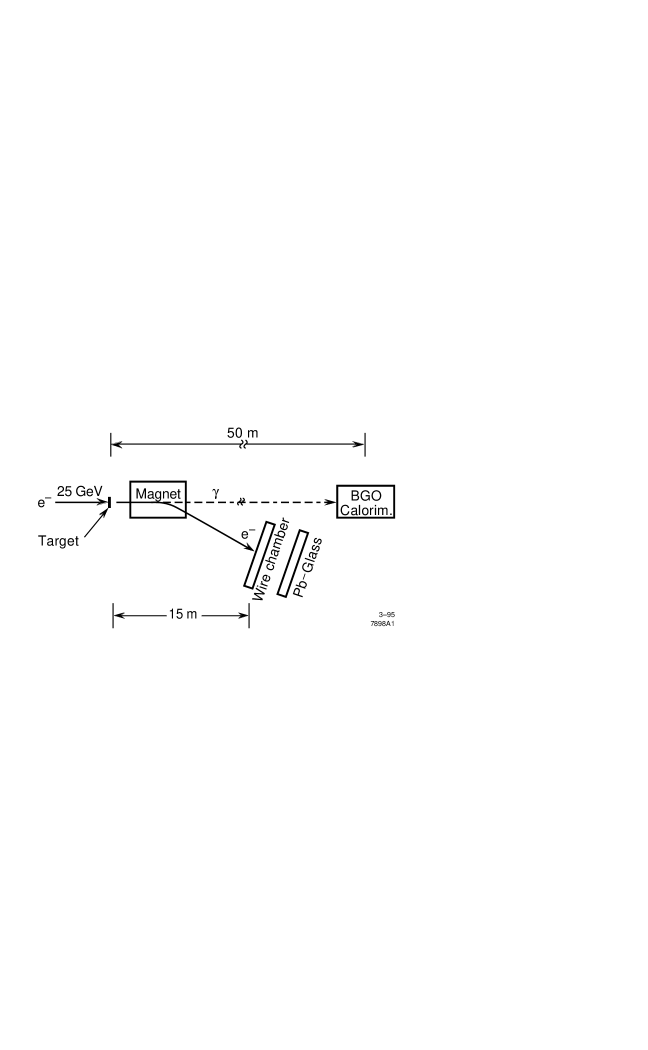
FIG. 2.: A diagram of the experiment. The apparatus is described in detail in the text.

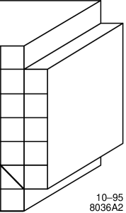
FIG. 3.: Drawing of the front of the calorimeter, showing bremsstrahlung plus transition radiation signal (dots) and synchrotron radiation background (hashes). The region below the diagonal solid lines is where the background rejection cut removes photon clusters from the data.

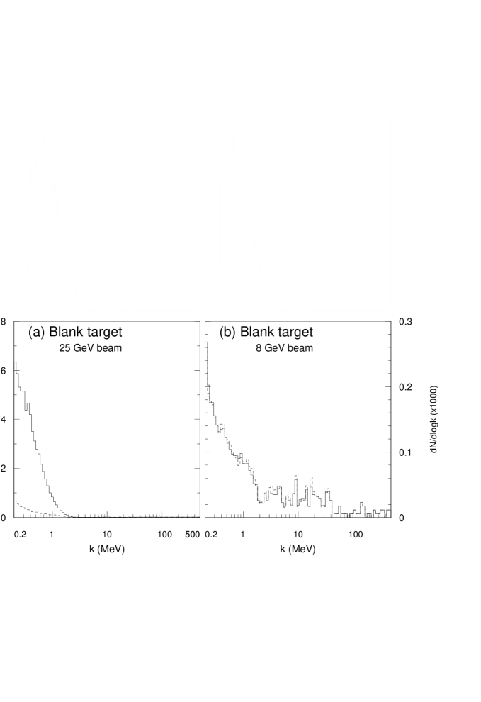
FIG. 4.: Data from the blank target runs at (a) 25 GeV and (b) 8 GeV. The units are photons per log($k$) per 1000 electrons. There are 25 bins per decade of photon energy, so each bin has width $\Delta k/k\sim 0.09$. The raw data are shown in the solid histogram, while the dashed lines show the data after the synchrotron radiation removal cut and efficiency correction. The cut removes about 90% of the data at 25 GeV, while at 8 GeV the efficiency only matches the geometrical expectation.

FIG. 5.: Measurements with statistical errors only of $dN/d(\log k)$ compared with the LPM plus dielectric effect plus transition radiation Monte Carlo curves (solid line), for our (a) 2% X₀ carbon and (b) 6% X₀ carbon targets in 25 GeV electron beams, while (d) shows the 2% X₀ carbon and (e) the 6% X₀ carbon target in the 8 GeV beam. The cross sections are given as $dN/d(\log k)/X_{0}$ where $N$ is the number of events per photon energy bin per incident electron. (c) shows the result of subtracting the data in (b) from that in (a), while (f) is the result of subtracting (e) from (d), as discussed in Section VI of the text. The curves are cut off where they go negative as a result of the procedure. Also shown are the Bethe-Heitler plus transition radiation MC (dashed line), LPM suppression only plus transition radiation (dotted line) and, for comparison, Bethe-Heitler without transition radiation (dot-dashed line). Figures 6 through 12 follow a similar format.

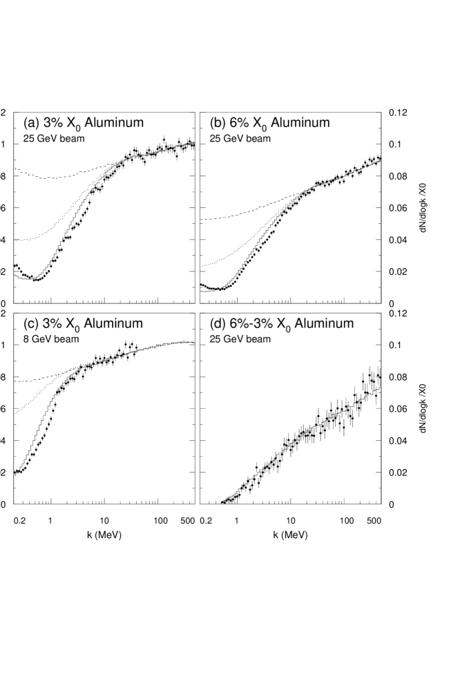
FIG. 6.: Measurements and Monte Carlo for our (a) 3% X₀ and (b) 6% X₀ aluminum targets at 25 GeV and (c) 3% X₀ at 8 GeV. (d) is the result of subtracting (b) from (a). The data and Monte Carlo formats and labels match Fig. 5, except that, for variety, the LPM suppression only simulation does not have transition radiation added.

FIG. 7.: Measurements and Monte Carlo for our (a) 3% X₀ and (b) 6% X₀ iron targets at 25 GeV and (c) 6% X₀ at 8 GeV, while (d) is the result of subtracting (b) from (a). Here, only an LPM plus dielectric suppression curve is shown.

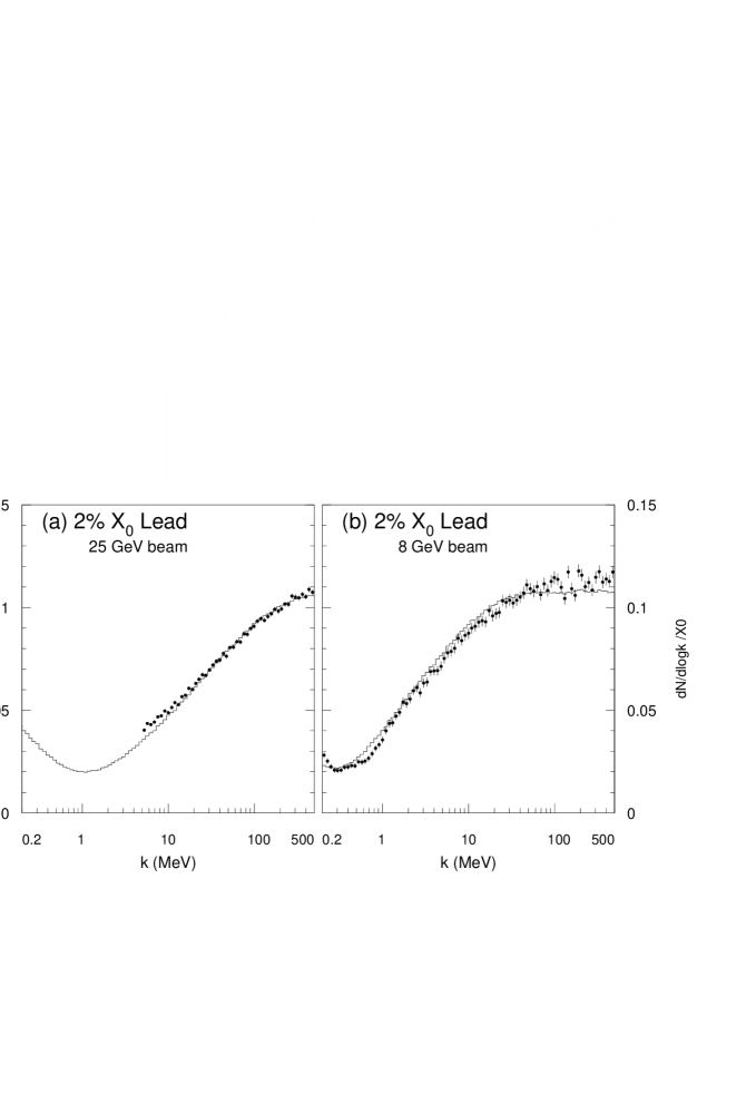
FIG. 8.: Measurements and Monte Carlo for our 2% X₀ lead target at (a) 25 GeV and (b) 8 GeV.

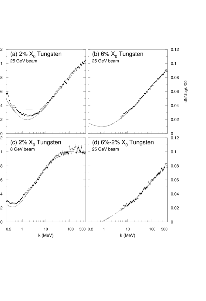
FIG. 9.: Measurements and Monte Carlo for our (a) 2% X₀ and (b) 6% X₀ tungsten targets at 25 GeV and (c) 2% X₀ at 8 GeV, while (d) is the result of subtracting (b) from (a). The flattening below 10 MeV is discussed in the text. The straight solid line in (a) between 1.5 and 2.7 MeV is the ‘single radiator’ calculation.

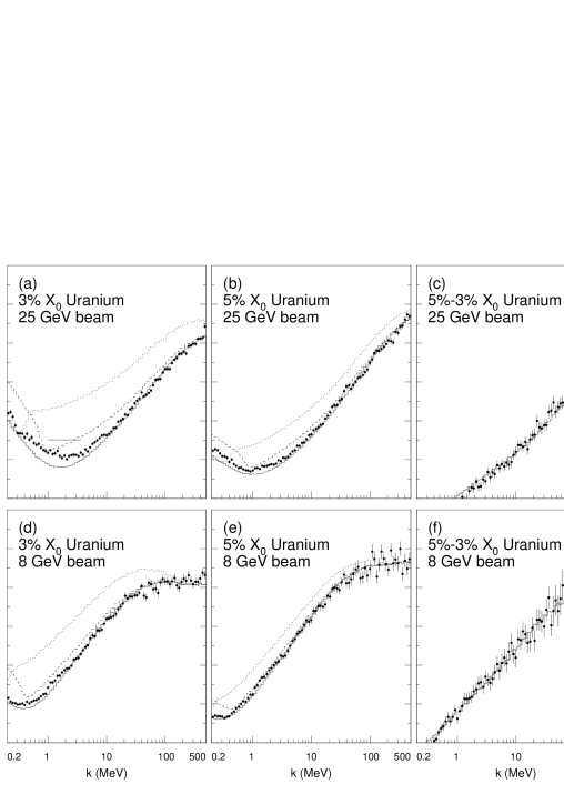
FIG. 10.: Measurements and Monte Carlo for our (a) 3% X₀ and (b) 5% X₀ uranium targets at 25 GeV and (d) 3% X₀ and (e) 5% X₀ uranium at 8 GeV, while (c) and (f) are the subtracted data. The solid line shows the standard Monte Carlo prediction. The horizontal solid line in (a) is from Eqn. 14. The dashed line includes the Pafomov transition radiation in the Monte Carlo, along with LPM and dielectric suppression. The dotted line is for the LPM and dielectric suppression plus the Ternovskii transition radiation with $\chi=1$.

FIG. 11.: Measurements and Monte Carlo for our (a) 0.7% X₀ and (b) 6% X₀ gold targets at 25 GeV and (d) 0.7% X₀ and (e) 6% X₀ gold at 8 GeV, with the subtracted data shown in (c) and (f).

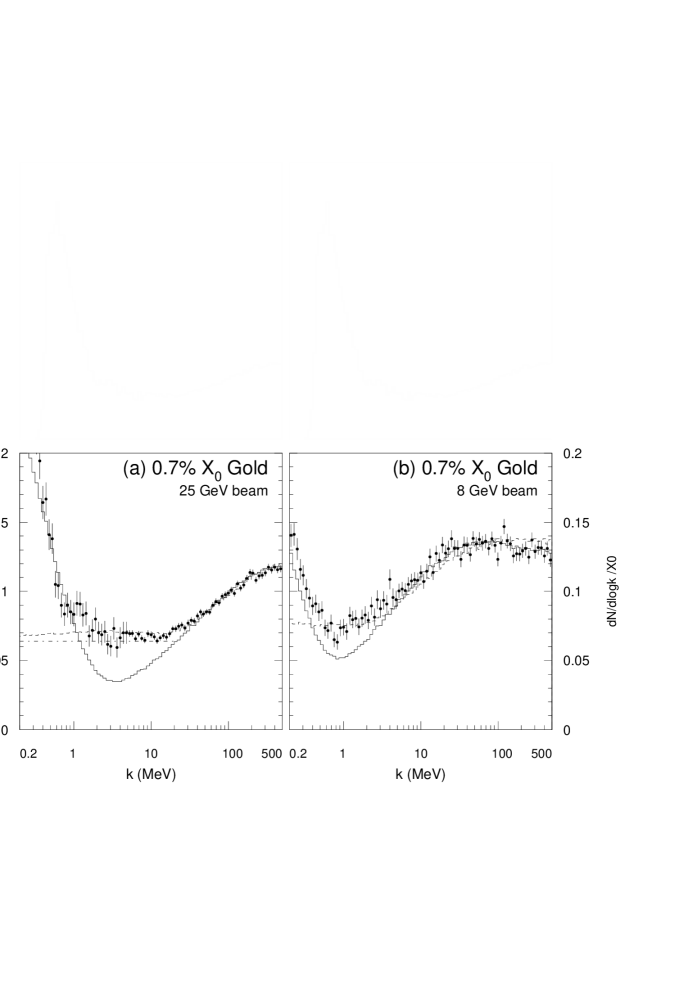
FIG. 12.: Expanded view of the 0.7% $X_{0}$ data at (a) 25 GeV and (b) 8 GeV, compared with the Blankenbecler and Drell prediction (dashed line), Shulga and Fomin prediction (dot-dashed line). For comparison, the standard MC is shown as the usual solid line.

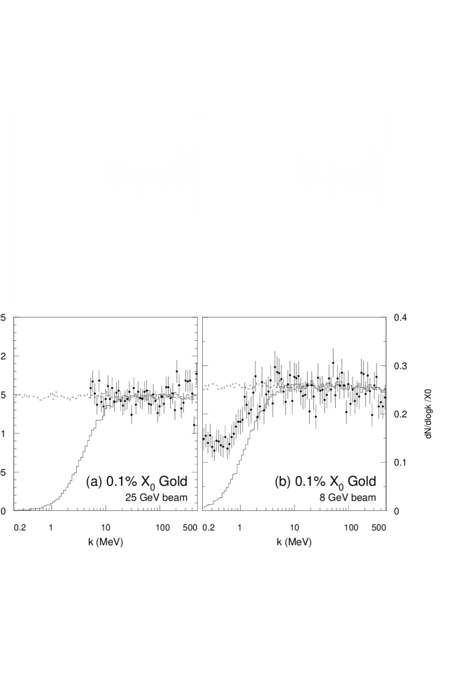
FIG. 13.: Measurements and Monte Carlo for our 0.1% X₀ gold target at (a) 25 GeV and (b) 8 GeV. The dashed line is the Bethe-Heitler prediction (no suppression), while the solid line is a Monte Carlo which includes dielectric suppression, but not LPM suppression. Because the very thin target should exhibit little transition radiation, no transition radiation is included in the Monte Carlo.

TABLE I.: $E_{LPM}$, $k_{LPM25}$, $k_{LPM8}$ and $r$ for the target materials used here.

Target	Z	$X_{0}$ (cm)	$E_{LPM}$ (TeV)	$k_{LPM25}$ (MeV)	$k_{LPM8}$(MeV)	$r$
Carbon	6	19.6	74	8.5	0.87	$5.5\times 10^{-5}$
Aluminum	13	8.9	36	15.7	1.6	$6.0\times 10^{-5}$
Iron	26	1.76	6.6	95	9.7	$1.0\times 10^{-4}$
Lead	82	0.56	2.1	295	30.1	$1.1\times 10^{-4}$
Tungsten	74	0.35	1.32	472	48.3	$1.5\times 10^{-4}$
Uranium	92	0.35	1.32	472	48.3	$1.4\times 10^{-4}$
Gold	79	0.33	1.25	500	51.2	$1.5\times 10^{-4}$

TABLE II.: List of target thicknesses and overall normalization constants. The target thicknesses $t$ are given in mm, gm/cm², and $X_{0}$. The last two columns give the normalization adjustments used to match the simulations with the data (statistical errors only).

Target	$t$		X0	Normalization	Normalization
-	(mm)	(g/cm2)	(%)	(% at 25 GeV)	(% at 8 GeV)
2% C	4.10	0.894	2.1	-3.0$\pm$0.3	-6.0$\pm$0.4
6% C	11.7	2.55	6.0	-2.9$\pm$0.2	-4.6$\pm$0.5
3% Al	3.12	0.842	3.5	-2.7$\pm$0.4	-3.0$\pm$0.4
6% Al	5.3	1.4	6.0	-2.8$\pm$0.3
3% Fe	0.49	0.39	2.8	-5.4$\pm$0.2	-1.4$\pm$0.4
6% Fe	1.08	0.85	6.1	-7.5$\pm$0.2
2% Pb	0.15	0.17	2.7	-4.5$\pm$0.2	-0.7$\pm$0.4
2% W	0.088	0.17	2.7	-8.3$\pm$0.3	-8.6$\pm$0.3
6% W	0.21	0.41	6.4	-4.7$\pm$0.3
3% U	0.079	0.15	2.2	-5.6$\pm$0.3	-6.3$\pm$0.3
5% U	0.147	0.279	4.2	-7.0$\pm$0.3	-7.5$\pm$0.4
0.1% Au	0.0038	0.0073	0.11
0.7% Au	0.023	0.044	0.70	-1.3$\pm$0.4	12.2$\pm$0.7
6% Au	0.20	0.39	6.0	-5.5$\pm$0.2	-5.0$\pm$0.3

TABLE III.: $\chi^{2}$ per degree of freedom of the fits to the subtracted data. The only free parameters were the absolute normalizations of the two individual targets. Typically, there were about 60 degrees of freedom. Statistical errors only were included in the fit.

Material	25 GeV	8 GeV
Carbon	2.74	1.17
Aluminum	0.84
Iron	2.32	1.41
Tungsten	0.99
Uranium	1.56	0.79
Gold	0.85	2.68

TABLE IV.: Table of Systematic Errors. The absolute column refers to the cross section for $k=500$MeV for both 8 and 25 GeV beams. The relative errors for $k<5$ MeV and $k>5$ MeV also apply to both 8 and 25 GeV beams, except for the synchrotron radiation removal cut, which is added in separately. Uncertainties in the theoretical calculation are not included.

Source		$k>5$MeV	$k<5$MeV
	Absolute	Relative	Relative
Energy Calibration	1%	1.5%	3%
Photon Cluster Finding		2%	7%
Calorimeter Nonlinearity	2%	3%	3%
Backgrounds		1%	4%
Target thickness	2%
Target Density		2%	2%
Electron Flux	0.5%	0.5%	0.5%
Monte Carlo	1.5%	1%	1.5%
Normalization Technique	1%
8 GeV Beam Total	3.5%	4.6%	9%
Synchrotron Radiation Removal			15%
25 GeV Beam Total	3.5%	4.6%	17%

REFERENCES

- [1] Present address: Institut de Fisica d’Altes Energies, Universitat Autonima de Barcelona, 08193 Bellaterra (Barcelona), Spain.
- [2] P. L. Anthony et al., Phys. Rev. Lett. 75, 1949 (1995).
- [3] P. L. Anthony et al. Phys. Rev. Lett. 76, 3550 (1996).
- [4] L. D. Landau and I. J. Pomeranchuk, Dokl. Akad. Nauk. SSSR 92, 535 (1953); 92, 735 (1953). These two papers are available in English in L. Landau, The Collected Papers of L. D. Landau, Pergamon Press, 1965.
- [5] A. B. Migdal, Phys. Rev. 103, 1811 (1956).
- [6] A. Misaki, Nucl. Phys B, Proc. Suppl., 33A,B. 192 (1993); Capdevielle and K. Atallah, Nucl. Phys. 28B (Proc. Suppl.), 90 (1992).
- [7] J. Learned, Phil. Trans. R. Soc. Lond. A346, 99 (1994);A. Misaki, Forschr. Phys. 38, 413 (1990).
- [8] X. N. Wang, M. Gyulassy and M. Plumer, Phys. Rev. D51, 3436 (1995); S. Brodsky and P. Hoyer, Phys. Lett. B298, 165 (1993).
- [9] G. Raffelt and D. Seckel, Phys. Rev. Lett. 67, 2605 (1991).
- [10] P. H. Fowler, D. H. Perkins and K. Pinkau, Phil. Mag. 4, 1030 (1959); E. Lohrmann, Phys. Rev. 122, 1908 (1961).
- [11] K. Kasahara, Phys. Rev. D31, 2737 (1985); S. C. Strausz et al., in Proc. 22nd Intl. Cosmic Ray Conf., Dublin, Ireland, Aug 11–23, 1991, 4, pg 233
- [12] A. Varfolomeev et al., Sov. Phys. JETP 42, 218 (1976).
- [13] J. F. Bak et al., Nucl. Phys. B302, 525 (1988).
- [14] J. Dolesji, J. Hüfner and B. Z. Kopeliovich, Phys. Lett. B312, 235 (1993).
- [15] F. R. Arutyunyan, A. A. Nazaryan and A. A. Frangyan, Sov. Phys. JETP 35, 1067 (1972).
- [16] J. D. Jackson, Classical Electrodynamics, 2nd ed. John Wiley & Sons, 1975, pg. 687.
- [17] B. Rossi, High Energy Particles, Prentice Hall, Inc., 1952, pg. 68.
- [18] M. L. Perl, in Proc. 1994 Les Rencontres de Physique de la Vallee D’Aoste, (Editions Frontieres, Gif-sur-Yvette, France, 1994). Ed. M. Grego, p. 567.
- [19] Y.-S. Tsai, Rev. Mod. Phys. 46, 815 (1974).
- [20] R. Blankenbecler and S. D. Drell, Phys. Rev. D53, 6265 (1996).
- [21] B. G. Zakharov, Pis’ma v. ZhETF 64, 737 (1996). B. G. Zakharov, Pis’ma v. ZhETF 63, 906 (1996).
- [22] M. L. Ter-Mikaelian, Dokl. Akad. Nauk. SSR 94, 1033 (1954). For a discussion in English, see M. L. Ter-Mikaelian, High Energy Electromagnetic Processes in Condensed Media, John Wiley & Sons, 1972.
- [23] V. M. Galitsky and I. I. Gurevich, Il Nuovo Cimento 32, 396 (1964).
- [24] Richard Blankenbecler, private communication.
- [25] I. I. Gol’dman, Sov. Phys. JETP 11, 1341 (1960).
- [26] N. F. Shul’ga and S. P. Fomin, JETP Lett. 63, 873 (1996).
- [27] F. F. Ternovskii, Sov. Phys. JETP 12, 123 (1960).
- [28] Particle Data Group, R.M.Barnett et al., Phys. Rev. D54, 1 (1996).
- [29] G. M. Garibyan, Sov. Phys. JETP 12, 237 (1961).
- [30] V. E. Pafomov, Sov. Phys. JETP 20, 253 (1965).
- [31] S. R. Klein et al., in Proc. XVI Int. Symp. Lepton and Photon Interactions at High Energies (Ithaca, 1993), Eds. P. Drell and D. Rubin, p. 172.
- [32] R. Becker-Szendy et al., in Proc. 21st SLAC Summer Institute on Particle Physics (Palo Alto, 1994), pg. 519.
- [33] P. Bosted and A. Rahbar, SLAC-NPAS-TN-85-1, February, 1985 (unpublished).
- [34] I. Kirkbride, in the SLAC Users Bulletin No. 97, Jan–May, 1984, pp 10–11.
- [35] M. Cavalli-Sforza et al., IEEE Trans. Nucl. Sci. 41, 1374 (1994).
- [36] A. Zucchiatti et al., Nucl. Instrum. & Meth. A281, 341 (1989).
- [37] T. Stanev et al., Phys. Rev. D25, 1291 (1982).
- [38] J. Hubbell, H. Gimm and I. Overbo, J. Phys. Chem. Ref. Data 9, 1023 (1980).
- [39] X. Artru, G. B. Yodh and G. Mennessier, Phys. Rev. D12, 1289 (1975).