SPIN STRUCTURE OF THE PROTON FROM POLARIZED INCLUSIVE DEEP–INELASTIC MUON–PROTON SCATTERING

We have measured the spin-dependent structure function $g_{1}^{\rm p}$ in inclusive deep-inelastic scattering of polarized muons off polarized protons, in the kinematic range $0.003<x<0.7$ and $1\,\mbox{GeV}^{2}<Q^{2}<60\,\mbox{GeV}^{2}$. A next-to-leading order QCD analysis is used to evolve the measured $g_{1}^{\rm p}(x,Q^{2})$ to a fixed $Q^{2}_{0}$. The first moment of $g_{1}^{\rm p}$ at $Q^{2}_{0}=10\,\mbox{GeV}^{2}$ is $\Gamma_{1}^{\rm p}=0.136\pm 0.013\,(\mbox{stat.})\pm 0.009\,(\mbox{syst.})\pm 0.005\,(\mbox{evol.})$. This result is below the prediction of the Ellis–Jaffe sum rule by more than two standard deviations. The singlet axial charge $a_{0}$ is found to be $0.28\pm 0.16$. In the Adler–Bardeen factorization scheme, $\Delta g\simeq 2$ is required to bring $\Delta\Sigma$ in agreement with the Quark-Parton Model. A combined analysis of all available proton and deuteron data confirms the Bjorken sum rule.

I INTRODUCTION

Deep-inelastic scattering of leptons from nucleons has revealed much of what is known about quarks and gluons. The scattering of high-energy charged polarized leptons on polarized nucleons provides insight into the spin structure of the nucleon at the parton level. The spin-dependent nucleon structure functions determined from these measurements are fundamental properties of the nucleon as are the spin-independent structure functions, and they provide crucial information for the development and testing of perturbative and non-perturbative Quantum Chromodynamics (QCD). Examples are the QCD spin-dependent sum rules and calculations by lattice gauge theory.

The first experiments on polarized electron–proton scattering were carried out by the E80 and E130 Collaborations at SLAC [1]. They measured significant spin-dependent asymmetries in deep-inelastic electron–proton scattering cross sections, and their results were consistent with the Ellis–Jaffe and Bjorken sum rules with some plausible models of proton spin structure. Subsequently, a similar experiment with a polarized muon beam and polarized proton target was made by the European Muon Collaboration (EMC) at CERN [2]. With a tenfold higher beam energy as compared to that at SLAC, the EMC measurement covered a much larger kinematic range than the electron scattering experiments and found the violation of the Ellis–Jaffe sum rule [3]. This implies, in the framework of the Quark-Parton Model (QPM), that the total contribution of the quark spins to the proton spin is small.

This result was a great surprise and posed a major problem for the QPM, particularly because of the success of the QPM in explaining the magnetic moments of hadrons in terms of three valence quarks. It stimulated a new series of polarized electron and muon nucleon scattering experiments which by now have achieved the following:

1. inclusive scattering measurements of the spin-dependent structure function $g_{1}^{\rm p}$ of the proton with improved accuracy over an enlarged kinematic range;

2. evaluation of the first moment of the proton spin structure function, $\Gamma_{1}^{\rm p}=\int_{0}^{1}g_{1}^{\rm p}(x){\rm d}x$, with reduced statistical and systematic errors;

3. similar measurements with polarized deuteron and ³He targets, in order to measure the neutron spin structure function and test the fundamental Bjorken sum rule for $\Gamma_{1}^{\rm p}-\Gamma_{1}^{\rm n}$ [4];

4. measurements of the spin-dependent structure function $g_{2}$ for the proton and neutron;

5. semi-inclusive measurements of final states which allow determination of the separate valence and sea quark contributions to the nucleon spin.

The recent measurements of polarized muon-nucleon scattering have been done by the Spin Muon Collaboration (SMC) at CERN with polarized muon beams of 100 GeV and 190 GeV obtained from the CERN SPS 450 GeV proton beam and with polarized proton and deuteron targets. Spin-dependent cross section asymmetries are measured over a wide kinematic range with relatively high $Q^{2}$ and extending to low $x$ values. The determination of $g_{1}(x,Q^{2})$ for the proton and deuteron has been the principal result of the SMC experiment, but $g_{2}$ and semi-inclusive measurements have also been made.

The recent measurements of polarized electron-nucleon scattering have been done principally at SLAC in experiment E142 [5] (beam energy $E_{e}\sim 19,23,26~{}{\rm GeV}$, ³He target), E143 [6, 7] (beam energy $E_{e}\sim 9,16,29~{}{\rm GeV}$, H and D targets) and E154 ($E_{e}\sim 48~{}{\rm GeV}$, ³He target). SLAC E155 with $E_{e}\sim 50~{}{\rm GeV}$ and polarized proton and deuteron targets will take data soon. The SLAC experiments provide inclusive measurements of $g_{1}$ and $g_{2}$ over a kinematic range of relatively low $Q^{2}$ and do not extend to very low $x$ values. However, the electron scattering experiments involve very high beam intensities and achieve excellent statistical accuracies. Hence the electron and the muon experiments are complementary. Recently the HERMES experiment at DESY has become operational and has reported preliminary results with a polarized ³He target [8]. This experiment uses a polarized electron beam of $27\,\mbox{GeV}$ in the electron ring at HERA and an internal polarized gas target. Both inclusive and semi-inclusive data were obtained, and polarized H and D targets will be used in the future.

In this paper, we present SMC results on the spin-dependent structure functions $g_{1}^{\rm p}$ and $g_{2}^{\rm p}$ of the proton, obtained from data taken in 1993 with a polarized butanol target. First results from these measurements were published in Refs. [9, 10]. We use here the same data sample but present a more refined analysis; in particular, we allow for a $Q^{2}$-evolution of the $g_{1}^{\rm p}$ structure function as predicted by perturbative QCD. SMC has also published results on the deuteron structure function $g_{1}^{\rm d}$ [11, 12, 13] and on a measurement of semi-inclusive cross section asymmetries [14]. For a test of the Bjorken sum rule we refer to our measurement of $g_{1}^{\rm d}$.

The paper is organized as follows. In Section II, we review the theoretical background. The experimental set-up and the data-taking procedure are described in Section III. In Section IV we discuss the analysis of cross section asymmetries and in Section V we give the evaluation of the spin-dependent structure function $g_{1}^{\rm p}$ and its first moment. The results for $g_{2}^{\rm p}$ are discussed in Section VI. In Section VII we combine proton and deuteron results to determine the structure function $g_{1}^{\rm n}$ of the neutron and to test the Bjorken sum rule. In Section VIII we interpret our results in terms of the spin structure of the proton. Finally, we present our conclusions in Section IX.

II THEORETICAL OVERVIEW

A The cross sections for polarized lepton-nucleon scattering

The polarized deep-inelastic lepton–nucleon inclusive scattering cross section in the one-photon exchange approximation can be written as the sum of a spin-independent term $\bar{\sigma}$ and a spin-dependent term $\Delta\sigma$ and involves the lepton helicity $h_{\ell}=\pm 1$:

$$\sigma=\bar{\sigma}-\frac{1}{2}h_{\ell}\Delta\sigma.$$ (1)

For longitudinally polarized leptons the spin $\bf{S_{\ell}}$ is along the lepton momentum $\bf{k}$. The spin-independent cross section for parity-conserving interactions can be expressed in terms of two unpolarized structure functions $F_{1}$ and $F_{2}$. These functions depend on the four momentum transfer squared $Q^{2}$ and the scaling variable $x=Q^{2}/2M\nu$, where $\nu$ is the energy of the exchanged virtual photon, and $M$ is the nucleon mass. The double differential cross section can be written as a function of $x$ and $Q^{2}$ [15]:

$$\frac{{\rm d^{2}}\bar{\sigma}}{{\rm d}x{\rm d}Q^{2}}=\frac{4{\pi}{\alpha}^{2}}{Q^{4}x}\Biggl{[}xy^{2}(1-\frac{2m_{\ell}^{2}}{Q^{2}})F_{1}(x,Q^{2})+$$ (2)

$$(1-y-\frac{{\gamma}^{2}y^{2}}{4})F_{2}(x,Q^{2})\Biggr{]},$$ (3)

where $m_{\ell}$ is the lepton mass, $y=\nu/E$ in the laboratory system, and

$$\gamma={2Mx\over\sqrt{Q^{2}}}={\sqrt{Q^{2}}\over\nu}.$$ (4)

The spin-dependent part of the cross section can be written in terms of two structure functions $g_{1}$ and $g_{2}$ which describe the interaction of lepton and hadron currents. When the lepton spin and the nucleon spin form an angle $\psi$, it can be expressed as [16]

$$\Delta\sigma=\cos\psi\,\Delta\sigma_{\parallel}+\sin\psi\,\cos\phi\,\Delta\sigma_{\perp},$$ (5)

where $\phi$ is the azimuthal angle between the scattering plane and the spin plane (Fig. 1).

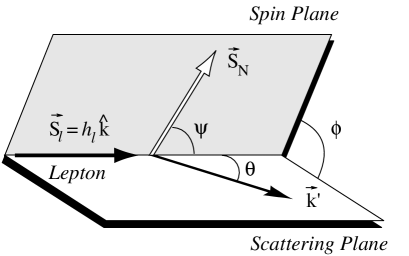
FIG. 1.: Lepton and nucleon kinematic variables in polarized lepton scattering on a fixed polarized nucleon target.

The cross sections $\Delta\sigma_{\parallel}$ and $\Delta\sigma_{\perp}$ refer to the two configurations where the nucleon spin is (anti)parallel or orthogonal to the lepton spin; $\Delta\sigma_{\parallel}$ is the difference between the cross sections for antiparallel and parallel spin orientations and $\Delta\sigma_{\perp}=-h_{\ell}\Delta\sigma_{\rm T}/\cos\phi$, the difference between the cross sections at angles $\phi$ and $\phi+\pi$. The corresponding differential cross sections are given by

$$\frac{{\rm d}^{2}\Delta\sigma_{\parallel}}{{\rm d}x{\rm d}Q^{2}}=\frac{16\pi\alpha^{2}y}{Q^{4}}\Biggl{[}(1-{y\over 2}-{\gamma^{2}y^{2}\over 4})g_{1}-{\gamma^{2}y\over 2}g_{2}\Biggr{]},$$ (6)

and

$$\frac{{\rm d}^{3}\Delta\sigma_{\rm T}}{{\rm d}x{\rm d}Q^{2}{\rm d}\phi}=-\cos\phi\,\frac{8\alpha^{2}y}{Q^{4}}\,\gamma\,\sqrt{1-y-{\gamma^{2}y^{2}\over 4}}\Biggl{(}{y\over 2}g_{1}+g_{2}\Biggr{)}.$$ (7)

For a high beam energy $E$, $\gamma$ is small since either $x$ is small or $Q^{2}$ large. The structure function $g_{1}$ is therefore best measured in the (anti)parallel configuration where it dominates the spin-dependent cross section; $g_{2}$ is best obtained from a measurement in the orthogonal configuration, combined with a measurement of $g_{1}$. In all formulae used in this article we consider only the single virtual-photon exchange. The interference effects between virtual Z⁰ and photon exchange in deep-inelastic muon scattering have been measured [17] and found to be small and compatible with the standard model expectations. They can be neglected in the kinematic range of current experiments.

B The cross section asymmetries

The spin-dependent cross section terms, Eqs. (6) and (7), make only a small contribution to the total deep-inelastic scattering cross section and furthermore their contribution is, in general, reduced by incomplete beam and target polarizations. Therefore they can best be determined from measurements of cross section asymmetries in which the spin-independent contribution cancels. The relevant asymmetries are

$$A_{\parallel}={\Delta\sigma_{\parallel}\over 2\bar{\sigma}},\hskip 28.45274ptA_{\perp}={\Delta\sigma_{\perp}\over 2\bar{\sigma}},$$ (8)

which are related to the virtual photon-proton asymmetries $A_{1}$ and $A_{2}$ by

$$A_{\parallel}=D(A_{1}+\eta A_{2}),\hskip 28.45274ptA_{\perp}=d(A_{2}-\xi A_{1}),$$ (9)

where

$$A_{1} = \frac{\sigma_{1/2}-\sigma_{3/2}}{\sigma_{1/2}+\sigma_{3/2}}=\frac{g_{1}-\gamma^{2}\,g_{2}}{F_{1}},$$ (10)

$$A_{2} = \frac{2\sigma^{\rm TL}}{\sigma_{1/2}+\sigma_{3/2}}=\gamma\frac{g_{1}+g_{2}}{F_{1}}.$$ (11)

In Eqs. (9) and (10), $D$ is the depolarization factor of the virtual photon defined below and $d$, $\eta$ and $\xi$ are the kinematic factors:

$$d = \frac{\sqrt{1-y-\gamma^{2}y^{2}/4}}{1-y/2}\,D,$$ (12)

$$\eta = \frac{\gamma(1-y-\gamma^{2}y^{2}/4)}{(1-y/2)(1+\gamma^{2}y/2)},$$ (13)

$$\xi = \frac{\gamma(1-y/2)}{1+\gamma^{2}y/2}~{}.$$ (14)

The cross sections $\sigma_{1/2}$ and $\sigma_{3/2}$ refer to the absorption of a transversely polarized virtual photon by a polarized proton for total photon–proton angular momentum component along the virtual photon axis of 1/2 and 3/2, respectively; $\sigma^{\rm TL}$ is an interference cross section due to the helicity spin-flip amplitude in forward Compton scattering [18]. The depolarization factor $D$ depends on $y$ and on the ratio $R=\sigma_{\rm L}/\sigma_{\rm T}$ of longitudinal and transverse photoabsorption cross sections:

$$D=\frac{y(2-y)(1+\gamma^{2}y/2)}{y^{2}(1+\gamma^{2})(1\!-\!2m_{\ell}^{2}/Q^{2})\!+\!\!2(1\!-\!y\!-\!\gamma^{2}y^{2}/4)(1\!+\!R)}~{}.$$ (15)

From Eqs. (9) and (10), we can express the virtual photon-proton asymmetry $A_{1}$ in terms of $g_{1}$ and $A_{2}$ and find the following relation for the longitudinal asymmetry:

$$\frac{A_{\parallel}}{D}=(1+\gamma^{2})\frac{g_{1}}{F_{1}}+(\eta-\gamma)A_{2}.$$ (16)

The virtual-photon asymmetries are bounded by positivity relations $|A_{1}|\leq 1$ and $|A_{2}|\leq\sqrt{R}$ [19]. When the term proportional to $A_{2}$ is neglected in Eqs. (9) and (16), the longitudinal asymmetry is related to $A_{1}$ and $g_{1}$ by

$$A_{1}\simeq\frac{A_{\parallel}}{D},\hskip 42.67912pt\frac{g_{1}}{F_{1}}\simeq\frac{1}{1+\gamma^{2}}\,\frac{A_{\parallel}}{D},$$ (17)

respectively, where $F_{1}$ is usually expressed in terms of $F_{2}$ and $R$:

$$F_{1}=\frac{1+\gamma^{2}}{2\,x\,(1+R)}{F_{2}}.$$ (18)

These relations are used in the present analysis for the evaluation of $g_{1}$ in bins of $x$ and $Q^{2}$, starting from the asymmetries measured in the parallel spin configuration and using parametrizations of $F_{2}(x,Q^{2})$ and $R(x,Q^{2})$.

The virtual photon-proton asymmetry $A_{2}$ is evaluated from the measured transverse and longitudinal asymmetries $A_{\parallel}$ and $A_{\perp}$:

$$A_{2}=\frac{1}{1+\eta\xi}\left(\frac{A_{\perp}}{d}+\xi\frac{A_{\parallel}}{D}\right).$$ (19)

From Eqs. (4) and (10), $A_{2}$ has an explicit $1/\sqrt{Q^{2}}$ dependence and is therefore expected to be small at high energies. The structure function $g_{2}$ is obtained from the measured asymmetries using Eqs. (10) and (19).

C The spin-dependent structure function $g_{1}$

The significance of the spin-dependent structure function $g_{1}$ can be understood from the virtual photon asymmetry $A_{1}$. As shown in Eq. (10), $A_{1}\simeq g_{1}/F_{1}$, or $\sigma_{1/2}-\sigma_{3/2}\propto g_{1}$. In order to conserve angular momentum, a virtual photon with helicity $+1$ or $-1$ can only be absorbed by a quark with a spin projection of $-\frac{1}{2}$ or $+\frac{1}{2}$, respectively, if the quarks have no orbital angular momentum. Hence, $g_{1}$ contains information on the quark spin orientations with respect to the proton spin direction.

In the simplest Quark-Parton Model (QPM), the quark densities depend only on the momentum fraction $x$ carried by the quark, and $g_{1}$ is given by

$$g_{1}(x)={\textstyle\frac{1}{2}}\sum_{i=1}^{n_{f}}e_{i}^{2}\Delta q_{i}(x),$$ (20)

where

$$\Delta q_{i}(x)=q_{i}^{+}(x)-q_{i}^{-}(x)+\bar{q}_{i}^{~{}+}(x)-\bar{q}_{i}^{~{}-}(x),$$ (21)

$q_{i}^{+}(\bar{q}_{i}^{~{}+})$ and $q_{i}^{-}(\bar{q}_{i}^{~{}-})$ are the distribution functions of quarks (antiquarks) with spin parallel and antiparallel to the nucleon spin, respectively, $e_{i}$ is the electric charge of the quarks of flavor $i$; and $n_{f}$ is the number of quark flavors involved.

In QCD, quarks interact by gluon exchange which gives rise to a weak $Q^{2}$ dependence of the structure functions. The treatment of $g_{1}$ in perturbative QCD follows closely that of unpolarized parton distributions and structure functions [20]. At a given scale $Q^{2}$, $g_{1}$ is related to the polarized quark and gluon distributions by coefficient functions $C_{q}$ and $C_{g}$ through [20]

$$g_{1}(x,t) = {\textstyle\frac{1}{2}}\sum_{k=1}^{n_{f}}\frac{e_{k}^{2}}{n_{f}}\int_{x}^{1}\frac{{\rm d}y}{y}\Bigl{[}C_{q}^{\rm S}({\textstyle\frac{x}{y}},\alpha_{s}(t))\Delta\Sigma(y,t)$$ (22)

$$+ 2n_{f}C_{g}({\textstyle\frac{x}{y}},\alpha_{s}(t))\Delta g(y,t)$$ (23)

$$+ C_{q}^{\rm NS}({\textstyle\frac{x}{y}},\alpha_{s}(t))\Delta q^{\rm NS}(y,t)\Bigr{]}.$$ (24)

In this equation, $t=\ln(Q^{2}/\Lambda^{2})$, $\alpha_{s}$ is the strong coupling constant, and $\Lambda$ is the scale parameter of QCD. The superscripts S and NS, respectively, indicate flavor-singlet and non-singlet parton distributions and coefficient functions; $\Delta g(x,t)$ is the polarized gluon distribution and $\Delta\Sigma$ and $\Delta q^{\rm NS}$ are the singlet and non-singlet combinations of the polarized quark and antiquark distributions

$$\Delta\Sigma(x,t) = \sum_{i=1}^{n_{f}}\Delta q_{i}(x,t),$$ (25)

$$\Delta q^{\rm NS}(x,t) = {{\displaystyle\sum_{i=1}^{n_{f}}}\left(e_{i}^{2}-{\displaystyle{1\over n_{f}}}{\displaystyle\sum_{k=1}^{n_{f}}}e_{k}^{2}\right)\over{\displaystyle{1\over n_{f}}}{\displaystyle\sum_{k=1}^{n_{f}}}{e_{k}^{2}}}\Delta q_{i}(x,t).$$ (26)

The $t$ dependence of the polarized quark and gluon distributions follows the Gribov–Lipatov–Altarelli–Parisi (GLAP) equations [21, 22]. As for the unpolarized distributions, the polarized singlet and gluon distributions are coupled by

$${{\rm d}\over{\rm d}t}\Delta\Sigma(x,t) = \frac{\alpha_{s}(t)}{2\pi}\int_{x}^{1}\frac{{\rm d}y}{y}\Bigl{[}P_{qq}^{\rm S}({{\textstyle\frac{x}{y}}},\alpha_{s}(t))\Delta\Sigma(y,t)$$ (27)

$$+ 2n_{f}P_{qg}({{\textstyle\frac{x}{y}}},\alpha_{s}(t))\Delta g(y,t)\Bigr{]},$$ (28)

$${{\rm d}\over{\rm d}t}\Delta g(x,t) = \frac{\alpha_{s}(t)}{2\pi}\int_{x}^{1}\frac{{\rm d}y}{y}\Bigl{[}P_{gq}({{\textstyle\frac{x}{y}}},\alpha_{s}(t))\Delta\Sigma(y,t)$$ (29)

$$+ P_{gg}({{\textstyle\frac{x}{y}}},\alpha_{s}(t))\Delta g(y,t)\Bigr{]},$$ (30)

whereas the non-singlet distribution evolves independently of the singlet and gluon distributions:

$${{\rm d}\over{\rm d}t}\Delta q^{\rm NS}(x,t)=\frac{\alpha_{s}(t)}{2\pi}\int_{x}^{1}\frac{{\rm d}y}{y}\,P_{qq}^{\rm NS}({\textstyle\frac{x}{y}},\alpha_{s}(t))\Delta q^{\rm NS}(y,t).$$ (31)

Here, $P_{ij}$ are the QCD splitting functions for polarized parton distributions.

Expressions (24), (27), (30) and (31) are valid in all orders of perturbative QCD. The quark and gluon distributions, coefficient functions, and splitting functions depend on the mass factorization scale and on the renormalization scale; we adopt here the simplest choice, setting both scales equal to $Q^{2}$. At leading order, the coefficient functions are

$$C_{q}^{0,\rm S}(\textstyle\frac{x}{y},\alpha_{s}) = C_{q}^{0,\rm NS}(\textstyle\frac{x}{y},\alpha_{s})=\delta(1-\textstyle\frac{x}{y}),$$ (32)

$$C_{g}^{0}(\textstyle\frac{x}{y},\alpha_{s}) = 0~{}.$$ (33)

Note that $g_{1}$ decouples from $\Delta g$ in this scheme.

Beyond leading order, the coefficient functions and the splitting functions are not uniquely defined; they depend on the renormalization scheme. The complete set of coefficient functions has been computed in the $\overline{\rm MS}$ renormalization scheme up to order $\alpha_{s}^{2}$ [23]. The ${\cal{O}}(\alpha_{s}^{2})$ corrections to the polarized splitting functions $P_{qq}$ and $P_{qg}$ have been computed in Ref. [23] and those to $P_{gq}$ and $P_{gg}$ in [24, 25]. This formalism allows a complete Next-to-Leading Order (NLO) QCD analysis of the scaling violations of spin-dependent structure functions.

In QCD, the ratio $g_{1}/F_{1}$ is $Q^{2}$-dependent because the splitting functions, with the exception of $P_{qq}$, are different for polarized and unpolarized parton distributions. Both $P_{gq}$ and $P_{gg}$ are different in the two cases because of a soft gluon singularity at $x=0$ which is only present in the unpolarized case. However, in kinematic regions dominated by valence quarks, the $Q^{2}$ dependence of $g_{1}/F_{1}$ is expected to be small [26].

D The small-$x$ behavior of $g_{1}$

The most important theoretical predictions for polarized deep-inelastic scattering are the sum rules for the nucleon structure functions $g_{1}$. The evaluation of the first moment of $g_{1}$,

$$\Gamma_{1}(Q^{2})=\int_{0}^{1}g_{1}(x,Q^{2})\/{\rm d}x,$$ (34)

requires knowledge of $g_{1}$ over the entire $x$ region. Since the experimentally accessible $x$ range is limited, extrapolations to $x=0$ and $x=1$ are unavoidable. The latter is not critical because it is constrained by the bound $|A_{1}|\leq 1$ and gives only a small contribution to the integral. However, the small-$x$ behavior of $g_{1}(x)$ is theoretically not well established and evaluation of $\Gamma_{1}$ depends critically on the assumption made for this extrapolation.

From the Regge model it is expected that for $Q^{2}\ll 2M\nu$, i.e. $x\rightarrow 0$, $g_{1}^{\rm p}+g_{1}^{\rm n}$ and $g_{1}^{\rm p}-g_{1}^{\rm n}$ behave like $x^{-\alpha}$ [27], where $\alpha$ is the intercept of the lowest contributing Regge trajectories. These trajectories are those of the pseudovector mesons $f_{1}$ for the isosinglet combination, $g_{1}^{\rm p}+g_{1}^{\rm n}$ and of $a_{1}$ for the isotriplet combination, $g_{1}^{\rm p}-g_{1}^{\rm n}$, respectively. Their intercepts are negative and assumed to be equal, and in the range $-0.5<\alpha<0$. Such behavior has been assumed in most analyses.

A flavor singlet contribution to $g_{1}(x)$ that varies as $(2\ln\frac{1}{x}-1)$ [28] was obtained from a model where an exchange of two nonperturbative gluons is assumed. Even very divergent dependences like $g_{1}(x)\propto(x\ln^{2}x)^{-1}$ were considered  [29]. Such dependences are not necessarily consistent with the QCD evolution equations.

Expectations based on QCD calculations for the behavior at small-$x$ of $g_{1}(x,Q^{2})$ are two-fold:

• resummation of standard Altarelli-Parisi corrections gives [30, 31, 32]

  $$g_{1}(x,Q^{2})\sim\exp\left[A\sqrt{\ln(\alpha_{x}(Q^{2}_{0})/\alpha_{s}(Q^{2}))\ln(1/x)}\right]~{},$$ (35)

  for the non-singlet and singlet parts of $g_{1}$.

• resummation of leading powers of $\ln 1/x$ gives

  $$g_{1}^{\rm NS}(x,Q^{2}) \sim x^{-w_{\rm NS}}\hskip 14.22636ptw_{\rm NS}\sim 0.4~{},$$ (36)

  $$g_{1}^{\rm S}(x,Q^{2}) \sim x^{-w_{\rm S}}\hskip 19.91684ptw_{\rm S}\sim 3w_{\rm NS}~{},$$ (37)

  for the non-singlet [33] and singlet [34] parts, respectively.

E Sum-rule predictions

1 The first moment of $g_{1}$ and the Operator Product Expansion

A powerful tool to study moments of structure functions is provided by the Operator Product Expansion (OPE), where the product of the leptonic and the hadronic tensors describing polarized deep-inelastic lepton–nucleon scattering reduces to the expansion of the product of two electromagnetic currents. At leading twist, the only gauge-invariant contributions are due to the non-singlet and singlet axial currents [35, 36]. If only the contributions from the three lightest quark flavors are considered, the axial current operator $A_{k}$ can be expressed in terms of the $\rm SU(3)$ flavor matrices $\lambda_{k}\,(k=1,\ldots,8)$ and $\lambda_{0}=2I$ as [36]

$$A_{\mu}^{k}=\overline{\psi}\frac{\lambda_{k}}{2}{\gamma_{5}}{\gamma_{\mu}}\psi,$$ (38)

and the first moment of $g_{1}$ is given by

$$s_{\mu}\Gamma_{1}^{\rm p(n)}(Q^{2}) = \frac{C^{\rm S}_{1}(Q^{2})}{9}\Bigl{[}\left\langle ps\right|A_{\mu}^{0}\left|ps\right\rangle\Bigr{]}$$ (39)

$$+ \frac{C^{\rm NS}_{1}(Q^{2})}{6}\Bigl{[}+(-)\left\langle ps\right|A_{\mu}^{3}\left|ps\right\rangle$$ (40)

$$+ \frac{1}{\sqrt{3}}\left\langle ps\right|A_{\mu}^{8}\left|ps\right\rangle\Bigr{]},$$ (41)

where $C^{\rm NS}_{1}$ and $C^{\rm S}_{1}$ are the non-singlet and singlet coefficient functions, respectively. The proton matrix elements for momentum $p$ and spin $s$, $\left\langle ps\right|A_{\mu}^{i}\left|ps\right\rangle$, can be related to those of the neutron by assuming isospin symmetry. In terms of the axial charge matrix element (axial coupling) for flavor $q_{i}$ and the covariant spin vector $s_{\mu}$,

$$s_{\mu}a_{i}(Q^{2})=\left\langle ps\right|\bar{q}_{i}{\gamma_{5}}{\gamma_{\mu}}q_{i}\left|ps\right\rangle,$$ (42)

they can be written as

$$\left\langle ps\right|A_{\mu}^{3}\left|ps\right\rangle = \frac{s_{\mu}}{2}a_{3}=\frac{s_{\mu}}{2}(a_{\mathrm{u}}-a_{\mathrm{d}})=\frac{s_{\mu}}{2}\left|\frac{g_{A}}{g_{V}}\right|,$$ (43)

$$\left\langle ps\right|A_{\mu}^{8}\left|ps\right\rangle = \frac{s_{\mu}}{2\sqrt{3}}a_{8}=\frac{s_{\mu}}{2\sqrt{3}}(a_{\mathrm{u}}+a_{\mathrm{d}}-2a_{\mathrm{s}}),$$ (44)

$$\left\langle ps\right|A_{\mu}^{0}\left|ps\right\rangle = s_{\mu}a_{0}=s_{\mu}(a_{\mathrm{u}}+a_{\mathrm{d}}+a_{\mathrm{s}}),$$ (45)

$$= s_{\mu}a_{0}(Q^{2}),$$ (46)

where the $Q^{2}$ dependence of $a_{u}$, $a_{d}$ and $a_{s}$ is implied from now on and is discussed in Section II F. The matrix element $a_{3}$ in Eq. (43) under isospin symmetry is equal to the neutron $\beta$-decay constant $g_{A}/g_{V}$. If exact $\rm SU(3)$ symmetry is assumed for the axial-flavor octet current, the axial couplings $a_{3}$ and $a_{8}$ in Eqs. (43) and (44) can be expressed in terms of coupling constants $F$ and $D$, obtained from neutron and hyperon $\beta$-decays [3], as

$$a_{3}=F+D\;\;\;\;\;\;\;\;a_{8}=3F-D.$$ (47)

The effects of a possible $\rm SU(3)$ symmetry breaking will be discussed in Section VIII B.

The first moment of the polarized quark distribution for flavor $q_{i}$, that is $\Delta q_{i}=\int\Delta q_{i}(x){\rm d}x$, is the contribution of flavor $q_{i}$ to the spin of the nucleon. In the QPM $a_{i}$ is interpreted as $\Delta q_{i}$ and $a_{0}$ as $\Delta\Sigma=\Delta u+\Delta d+\Delta s$. In this framework, the moments $a_{\mathrm{u}}$, $a_{\mathrm{d}}$, $a_{\mathrm{s}}$ $\ldots$ are bound by a positivity limit given by the corresponding moments of $u,d,s,\ldots$ obtained from unpolarized structure functions. In Section II F we will see that the $\rm U(1)$ anomaly modifies this simple interpretation of the axial couplings.

When $Q^{2}$ is above the charm threshold $(2m_{c})^{2}$, four flavors must be considered and an additional proton matrix element must be defined:

$$\left\langle ps\right|A_{\mu}^{15}\left|ps\right\rangle=\frac{s_{\mu}}{2\sqrt{6}}(a_{\mathrm{u}}+a_{\mathrm{d}}+a_{\mathrm{s}}-3a_{\mathrm{c}})=\frac{s_{\mu}}{2\sqrt{6}}a_{15},$$ (48)

while the singlet matrix element becomes $s_{\mu}(a_{\mathrm{u}}+a_{\mathrm{d}}+a_{\mathrm{s}}+a_{\mathrm{c}})$.

TABLE I.: Higher-order coefficients of the non-singlet and singlet coefficient functions $C_{1}^{\rm NS}$ and $C_{1}^{\rm S}$ in the $\overline{\rm MS}$ scheme. The coefficients $c_{4}^{\rm NS}$ and $c_{3}^{\rm S}$ are estimates; $c_{3}^{\rm S}$ is unknown for $n_{f}=4$ flavors. The quantities $a_{0}^{\infty}$ and $a_{0}(Q^{2})$ are discussed in Section II E 3.

$n_{f}$	non-singlet				singlet ($a_{0}^{\infty}$)			singlet ($a_{0}(Q^{2})$)
	$c_{1}^{\rm NS}$	$c_{2}^{\rm NS}$	$c_{3}^{\rm NS}$	$c_{4}^{\rm NS}$	$c_{1}^{\rm S}$	$c_{2}^{\rm S}$	$c_{3}^{\rm S}$	$c_{1}^{\rm S}$	$c_{2}^{\rm S}$	$c_{3}^{\rm S}$
3	1.0	3.5833	20.2153	130	0.3333	0.5496	2	1	1.0959	3.7
4	1.0	3.2500	13.8503	68	0.0400	$-1.0815$	—	1	$-0.0666$	—

2 The Bjorken sum rule

The Bjorken sum rule [4] is an immediate consequence of Eqs. (41) and (43). In the QPM where $C_{1}^{\rm NS}=1$,

$$\Gamma_{1}^{\rm p}-\Gamma_{1}^{\rm n}=\frac{1}{6}\left|\frac{g_{A}}{g_{V}}\right|.$$ (49)

In this form, the sum rule was first derived by Bjorken from current algebra and isospin symmetry, and has since been recognized as a cornerstone of the QPM.

The Bjorken sum rule is a rigorous prediction of QCD in the limit of infinite momentum transfer. It is subject to QCD radiative corrections at finite values of $Q^{2}$ [35, 37]. These QCD corrections have recently been computed up to ${\cal{O}}(\alpha_{s}^{3})$ [38] and the ${\cal{O}}(\alpha_{s}^{4})$ correction has been estimated [39]. Since the Bjorken sum rule is a pure flavor non-singlet expression, these corrections are given by the non-singlet coefficient function $C_{1}^{\rm NS}$:

$$\Gamma_{1}^{\rm p}-\Gamma_{1}^{\rm n}=\frac{1}{6}\left|\frac{g_{A}}{g_{V}}\right|C_{1}^{\rm NS}.$$ (50)

Beyond leading order, $C_{1}^{\rm NS}$ depends on the number of flavors and on the renormalization scheme. Table I shows the coefficients $c_{i}^{\rm NS}$ of the expansion

$$C_{1}^{\rm NS}=1-c_{1}^{\rm NS}\left(\frac{\alpha_{s}(Q^{2})}{\pi}\right)-c_{2}^{\rm NS}\left(\frac{\alpha_{s}(Q^{2})}{\pi}\right)^{2}$$ (51)

$$-c_{3}^{\rm NS}\left(\frac{\alpha_{s}(Q^{2})}{\pi}\right)^{3}-{\cal O}(c_{4}^{\rm NS})\left(\frac{\alpha_{s}(Q^{2})}{\pi}\right)^{4},$$ (52)

in the $\overline{\rm MS}$ scheme.

3 The Ellis–Jaffe sum rules

In the QPM the coefficient functions are equal to unity and assuming exact $\rm SU(3)$ symmetry (Eq. (47)) the expression (41) can be written:

$$\Gamma_{1}^{\rm p(n)}=+(-)\frac{1}{12}(F+D)+\frac{5}{36}(3F-D)+\frac{1}{3}a_{\mathrm{s}}~{}.$$ (53)

This relation was derived by Ellis and Jaffe [3]. With the additional assumption that $a_{\mathrm{s}}=0$, which in the QPM means $\Delta s=0$, they obtained numerical predictions for $\Gamma_{1}^{\rm p}$ and $\Gamma_{1}^{\rm n}$. The EMC measurement [2] showed that $\Gamma_{1}^{\rm p}$ is smaller than their prediction which in the QPM implied that $\Delta\Sigma$, the contribution of quark spins to the proton spin, is small. This result is at the origin of the current interest in polarized deep-inelastic scattering.

The moments of $g_{1}$ and the Ellis–Jaffe predictions are also subject to QCD radiative corrections. The coefficient function $C^{\rm NS}_{1}$ (Eq. (52)) used for the Bjorken sum rule also applies to the non-singlet part. The additional coefficient function $C_{1}^{\rm S}$ for the singlet contribution in Eq. (41) has been computed up to ${\cal{O}}(\alpha_{s}^{2})$ [36] and the ${\cal{O}}(\alpha_{s}^{3})$ term has also been estimated for $n_{f}=3$ flavors [40]:

$$C_{1}^{\rm S}=1-c_{1}^{\rm S}\left(\frac{\alpha_{s}(Q^{2})}{\pi}\right)-c_{2}^{\rm S}\left(\frac{\alpha_{s}(Q^{2})}{\pi}\right)^{2}$$ (54)

$$-{\cal{O}}(c_{3}^{\rm S})\left(\frac{\alpha_{s}(Q^{2})}{\pi}\right)^{3},$$ (55)

and the coefficients $c_{i}^{\rm S}$ are shown in Table I. The QCD-corrected Ellis–Jaffe predictions for $a_{s}=0$ become

$$\Gamma_{1}^{\rm p(n)}=C_{1}^{\rm NS}\left[+(-)\frac{1}{12}\left|\frac{g_{A}}{g_{V}}\right|+\frac{1}{36}(3F-D)\right]$$ (56)

$$+\frac{1}{9}C_{1}^{\rm S}(3F-D).$$ (57)

Since $a_{0}=a_{8}+3a_{\mathrm{s}}$, the assumption $a_{\mathrm{s}}=0$ is equivalent to $a_{0}=a_{8}=3F-D$. The quantity $3F-D$ is independent of $Q^{2}$, so the assumption $a_{0}=a_{8}$ should be made for $a_{0}^{\infty}=a_{0}(Q^{2}=\infty)$ [36] . The coefficients $c_{i}^{\rm S}$ in the third column of Table I should be used to compute the coefficient function $C_{1}^{\rm S}$ that appears in Eq. (56).

4 Higher twist effects

As for unpolarized structure functions, spin-dependent structure functions measured at small $Q^{2}$ are subject to higher twist (HT) effects due to nonperturbative contributions to the lepton–nucleon cross section. In the analysis of moments and for not too low $Q^{2}$, such effects are expressed as a power series in $1/Q^{2}$:

$$\Gamma_{1} = \frac{1}{2}a^{(0)}+\frac{M^{2}}{9Q^{2}}(a^{(2)}+4d^{(2)}+4f^{(2)})+{\cal{O}}\left({M^{4}\over Q^{4}}\right)$$ (58)

$$= \frac{1}{2}a^{(0)}+{\rm HT}.$$ (59)

Here $a^{(0,2)}$, $d^{(2)}$ and $f^{(2)}$ are the reduced matrix elements of the twist–2, twist–3 and twist–4 components, respectively, and $M$ is the nucleon mass. The values of $a^{(2)}$ and $d^{(2)}$ for proton and deuteron have recently been measured [41] from the second moment of $g_{1}$ and $g_{2}$, and found to be consistent with zero. Several authors have estimated the HT effects for $\Gamma_{1}$ [42, 43, 44] and for the Bjorken sum rule [45, 46]. In the literature, there is a consensus that such effects are probably negligible in the kinematic range of the data used to evaluate $\Gamma_{1}$ in this paper.

F The physical interpretation of $a_{0}$ and the $\rm U(1)$ anomaly

In the simplest approximation, the axial coupling $a_{0}(Q^{2})$ is expected to be equal to $\Delta\Sigma$, the contribution of the quark spin to the nucleon spin. However, in QCD the $\rm U(1)$ anomaly causes a gluon contribution to $a_{0}(Q^{2})$ [47, 48, 49] as well which makes $\Delta\Sigma$ dependent on the factorization scheme, while $a_{0}$ is not. The total fraction of the nucleon spin carried by quarks is the sum of $\Delta\Sigma$ and $L_{q}$, where $L_{q}$ is the contribution of quark orbital angular momentum to the nucleon spin. Recently, it was pointed out [50] that this sum is scheme-independent because of an exact compensation between the anomalous contribution to $\Delta\Sigma$ and to $L_{q}$.

The decomposition of $a_{0}$ into $\Delta\Sigma$ and a gluon contribution is scheme-dependent [51]. In the Adler–Bardeen (AB) [52] factorization scheme [53]

$$a_{0}(Q^{2})=\Delta\Sigma-n_{f}\frac{\alpha_{s}(Q^{2})}{2\pi}\Delta g(Q^{2}),$$ (60)

where the last term was originally identified as the anomalous gluon contribution [47, 48, 49]. In this scheme $\Delta\Sigma$ is independent of $Q^{2}$; however it cannot be obtained from the measured $a_{0}$ without an input value for $\Delta g$. In other schemes $\Delta\Sigma$ is equal to $a_{0}(Q^{2})$ but then it depends on $Q^{2}$ [51]. The differences between these two schemes do not vanish when $Q^{2}\rightarrow\infty$ because $\alpha_{s}(Q^{2})\Delta g$ remains finite when $Q^{2}\rightarrow\infty$ [47].

G The spin-dependent structure function $g_{2}$

Phenomenologically, the structure function $g_{2}$ can be understood from the spin-flip amplitude that gives rise to the interference asymmetry $A_{2}\propto g_{1}+g_{2}$ of Eq. (10), owing to the absorption of a longitudinally polarized photon by the nucleon. There are two mechanisms by which this can occur [54]. In the first, allowed in perturbative QCD, the photon is absorbed by a quark, causing its helicity to flip, but since helicity is conserved for massless fermions, this process is strongly suppressed for small quark masses. In the second, which is of a non-perturbative nature, the photon is absorbed by coherent parton scattering where the final-state quark conserves helicity by absorption of a helicity $-1$ gluon.

Wandzura and Wilczek have shown [55] that $g_{2}$ can be decomposed as

$$g_{2}(x,Q^{2})=g_{2}^{\rm WW}(x,Q^{2})+\bar{g}_{2}(x,Q^{2}).$$ (61)

The term $g_{2}^{\rm WW}$ is a linear function of $g_{1}$,

$$g_{2}^{\rm WW}(x,Q^{2})=-g_{1}(x,Q^{2})+\int_{x}^{1}g_{1}(t,Q^{2})\frac{{\rm d}t}{t}.$$ (62)

The term $\bar{g}_{2}$ is due to a twist-3 contribution in the OPE [16] and is a measure of quark–gluon correlations in the nucleon [56].

In the simplest QPM, $g_{2}$ vanishes because the masses and transverse momenta of quarks are neglected. The predictions of improved quark-parton models which take these aspects into account depend critically on the assumptions made for the quark masses and the nucleon wave function [56].

The Burkhardt–Cottingham sum rule predicts that the first moment of $g_{2}$ vanishes for both the proton and the neutron [57]:

$$\Gamma_{2}\equiv\int_{0}^{1}g_{2}(x){\rm d}x=0~{}.$$ (63)

This sum rule is derived in Regge theory and relies on assumptions that are not well established. Its validity has therefore been the subject of much debate in the recent theoretical literature [16, 58, 59].

III EXPERIMENTAL METHOD

A Overview

The experiment involves principally the measurement of cross section asymmetries for inclusive scattering of longitudinally polarized muons from polarized protons in a solid butanol target (Fig. 2). The energy of the incoming positive muons, $190~{}\,\mbox{GeV}$, is measured with a magnetic spectrometer in the Beam Momentum Station (BMS). The scattered muons are detected in the Forward Spectrometer (FS). They are identified by coincident hits in arrays of hodoscopes located upstream and downstream of a hadron absorber; their momenta are measured with a large-acceptance, high-resolution magnetic spectrometer. The beam polarization is measured with a polarimeter located downstream of the FS. The high energy of the beam provides a kinematic coverage down to $x\sim 0.003$ for $Q^{2}>1~{}{\rm GeV}^{2}$, and a high average $Q^{2}$. A small data sample was collected with a beam energy of 100 GeV and transverse target polarization for the measurement of the asymmetry $A^{\rm p}_{2}$.

The counting-rate asymmetries measured in this experiment vary from $0.001$ to $0.05$ depending on the kinematic region. To assure that the asymmetries measured do not depend on the incident muon flux, the polarized target is subdivided into two cells which are polarized in opposite directions. Frequent reversals of the target spin directions in both cells strongly reduce systematic errors arising from time-dependent variations of the detector efficiencies. Such errors are further reduced by the high redundancy of detectors in the forward spectrometer. The muon beam polarization is not reversed in this experiment.

The statistical errors of the counting-rate asymmetries are proportional to $(P_{\mu}P_{\rm t})^{-1}(N)^{-1/2}$, where $P_{\mu}$ and $P_{\rm t}$ are the beam and target polarizations, respectively, and $N$ is the number of events. Hence high values of $P_{\mu}$ and $P_{\rm t}$ as well as high $N$ are important.

B The muon beam

The SMC experiment (NA47) is installed in the upgraded muon beam M2 of the CERN SPS [60]. A beryllium target is bombarded with 450 GeV protons from the SPS and secondary pions and kaons are momentum-selected and transported through a 600 m long decay channel where for 200 GeV about 5 percent decay into muons and neutrinos. The remaining hadrons are stopped in a 9.9 m long beryllium absorber for the 190 GeV muon beam. Downstream of the absorber, muons are momentum selected and transported into the experimental hall.

The beam intensity was $4\times 10^{7}$ muons per SPS pulse; these pulses are 2.4 s long with a repetition period of 14.4 s. The beam spot on the target was approximately circular with a r.m.s. radius of 1.6 cm and a r.m.s. momentum width of $\approx 2.5\%$. The momentum of the incident muons is measured for each trigger in the BMS located upstream of the experimental hall (Fig. 2). The BMS employs a set of quadrupoles (Q) and a dipole (B6) in the beam line, with a nominal vertical deflection of 33.7 mrad. Four planes of fast scintillator arrays (HB) upstream and downstream of this magnet are used to measure the muon tracks. The resolution of the momentum measurement is better than 0.5%.

The beam is naturally polarized because of parity violation in the weak decays of the parent hadrons. For monochromatic muon and hadron beams, the polarization is a function of the ratio of muon and hadron energies [61]:

$$P_{\mu}=\pm\frac{m_{\pi,{\rm K}}^{2}+(1-\frac{2E_{\pi,{\rm K}}}{E_{\mu}})m_{\mu}^{2}}{m_{\pi,{\rm K}}^{2}-m_{\mu}^{2}},$$ (64)

where the $-$ and + signs refer to positive and negative muons, respectively (Fig. 3). For a given pion energy, the muon intensity depends on the ratio ${E_{\pi,{\rm K}}}/{E_{\mu}}$; this ratio was optimized using Monte Carlo simulations of the beam transport [62, 63] to obtain the best combination of beam polarization and intensity.

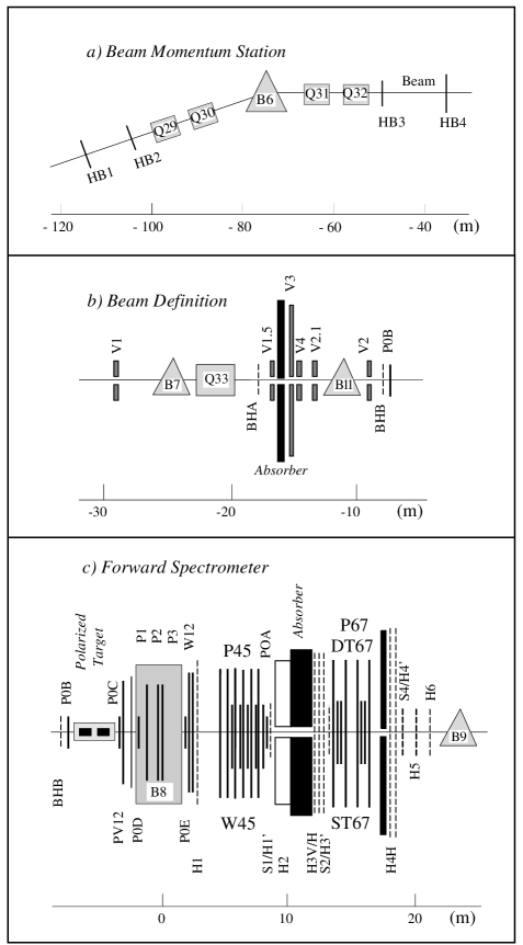
FIG. 2.: Schematic layout of the muon beam and forward spectrometer. The individual detectors are discussed in the text (see Table III). In (b), B11 is a compensating dipole that is used only when taking data with transverse target polarization. In (c), B8 is the forward spectrometer magnet and referred to as the FSM in the text. A right-handed coordinate system is used with its origin at the center of B8. The $x$-axis points along the beam direction, and the $z$-axis points upwards (out of the page in (b) and (c)).

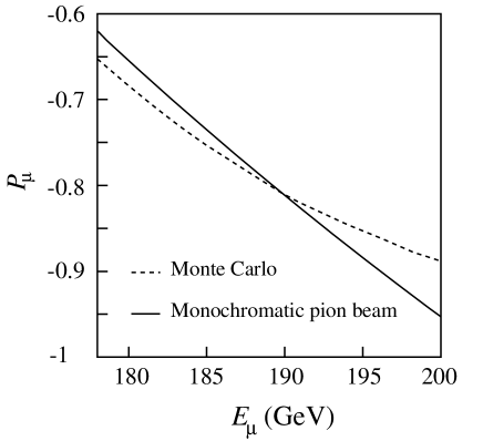
FIG. 3.: Muon polarization $P_{\mu}$ as a function of muon beam energy $E_{\mu}$ [60] for a monochromatic pion beam of 205 GeV (solid line)(Eq. (64)), and mean $P_{\mu}$ vs. $E_{\mu}$ as calculated by beam transport simulations [60] (dashed line).

C Measurement of the beam polarization

A polarimeter downstream of the muon spectrometer allows us to determine the beam polarization by two different methods. The first involves measuring the energy spectrum of positrons from muon decay in flight, $\mu^{+}\rightarrow\rm e^{+}\bar{\nu}_{\mu}\nu_{\rm e}$, which depends on the parent-muon polarization [64]. The second method involves measuring the spin-dependent cross section asymmetry for elastic scattering of polarized muons on polarized electrons [65]. The two methods require different layouts for the polarimeter, and thus cannot be run simultaneously.

1 Polarized-muon decay

The energy spectrum of positrons from the decay $\mu^{+}\rightarrow{\rm e}^{+}\nu_{{\rm e}}\bar{\nu}_{\mu}$ [66] can be expressed in terms of the ratio of positron and muon energies $y_{{\rm e}}=E_{{\rm e}}/E_{\mu}$ and of the muon polarization $P_{\mu}$ [67, 68]:

$$\frac{{\rm d}N}{{\rm d}y_{\rm e}}=N_{0}\left[\frac{5}{3}-3y_{\rm e}^{2}+\frac{4}{3}y_{\rm e}^{3}-P_{\mu}\left(\frac{1}{3}-3y_{\rm e}^{2}+\frac{8}{3}y_{\rm e}^{3}\right)\right],$$ (65)

where $N_{0}$ is the number of muon decays.

The polarimeter configuration for this measurement is shown in Fig. 4 (a). It consists of a 30 m long evacuated decay volume, followed by a magnetic spectrometer and an electromagnetic calorimeter to measure and identify the decay positrons. The beginning of the decay path is defined by the shower veto detector (SVD) which consists of a lead foil followed by two scintillator hodoscopes. Along the decay path, tracks are measured with multiwire proportional chambers (MWPC). The decay positrons are momentum analyzed in a magnetic spectrometer consisting of a 6 meter long small-aperture dipole magnet followed by another set of MWPC. This spectrometer and the BMS, which measures the parent muon momentum, were intercalibrated in dedicated runs to 0.2%. A lead glass calorimeter (LGC) is used to identify the decay positrons.

The trigger requires a hit in each SVD plane, in coincidence with a signal from the LGC above a threshold of about $15$ GeV. Events with two or more hits in both planes within a 50 ns time window are rejected. This suppresses background from incident positrons originating upstream of the polarimeter and rejects events with more than one muon.

In the off-line analysis, events whose energy $E_{\mu}$ was measured in the BMS and experienced a large energy loss in the SVD are rejected. A single track is required, both upstream and downstream of the magnet. To reject muon decays inside the magnetic field volume, the upstream and downstream tracks are required to intersect in the center of the magnet. Decay positrons are identified by requiring that the momentum measured by the polarimeter spectrometer matches the energy deposition in the LGC.

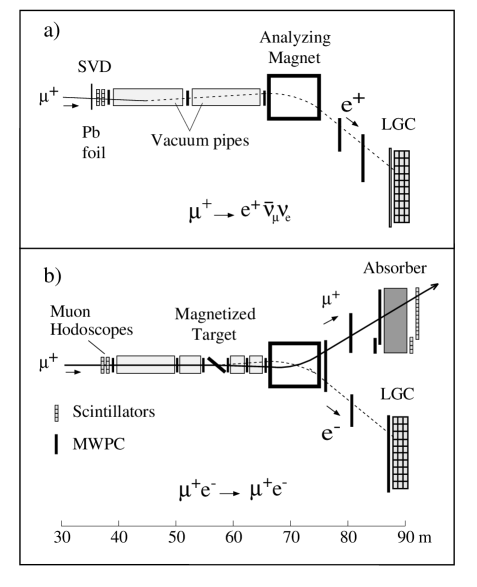
FIG. 4.: Schematic layout of the beam polarimeter for the muon decay measurement (a) and for the muon–electron scattering measurement (b). The different components of the apparatus are discussed in the text. The lead glass electromagnetic calorimeter and the shower veto detector are labeled as LGC and SVD, respectively.

The measured positron spectrum is corrected for the overall detector response. The response function is obtained from a Monte Carlo simulation that generates muons according to the measured beam phase space. The simulation accounts for radiative effects at the vertex and external bremsstrahlung, the geometry of the set-up, and chamber efficiencies. The Monte Carlo events were processed using the same procedure applied to the real data. The response function is obtained by dividing the Monte Carlo spectrum by the Michel spectrum of Eq. (65).

The polarization $P_{\mu}$ can be determined by fitting Eq. (65) to the measured decay spectrum corrected for the detector response. Figure 5 shows the sensitivity of the Michel spectrum to the muon polarization. The systematic error in the $P_{\mu}$ determination is mainly due to uncertainties in the response function, the main contributions to which are uncertainties in the MWPC efficiencies and in the background rejection. Background due to external $\gamma$-conversion, $\mu^{+}\rightarrow\mu^{+}\gamma\rightarrow\mu^{+}{\rm e}^{+}{\rm e}^{-}$, is measured using the charge-conjugate process with a $\mu^{-}$ beam and was found to be negligible. Other contributions to the systematic error arise from uncertainties in $y_{\rm e}$, in radiative effects at the vertex and in the alignment of the wire chambers.

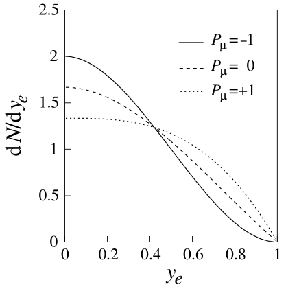
FIG. 5.: The Michel spectrum predictions for $P_{\mu}=-1,\,0,$ and $+1$ are shown by the solid, dashed and dotted lines, respectively.

           

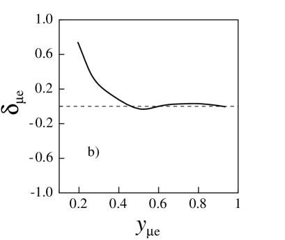
FIG. 6.: The QED radiative corrections to the asymmetry $A_{\mu\mathrm{e}}$ (a) without experimental cuts. (b) The asymmetry if the following experimental cuts are included in the calculation: (i) recoil electron energy greater than 35 GeV, (ii) energy difference between initial and final states less than 40 GeV, (iii) angular cuts on both outgoing muon and electron. The corrections $\delta_{\rm\mu e}$ are given in percent.

2 Polarized muon–electron scattering

In QED at first order, the differential cross section for elastic scattering of longitudinally polarized muons off longitudinally polarized electrons is [69]

$$\frac{{\rm d}\sigma}{{\rm d}y_{\rm\mu e}}=\frac{2{\pi}r^{2}_{\rm e}m_{\rm e}}{E_{\mu}}\left(\frac{1}{y_{\rm\mu e}^{2}}-\frac{1}{y_{\rm\mu e}Y}+\frac{1}{2}\right)(1+P_{\rm e}P_{\mu}A_{\mu{\rm e}}),$$ (66)

where $m_{\rm e}$ is the electron mass, $r_{\rm e}$ the classical electron radius, $y_{\rm\mu e}=1-E^{\prime}_{\mu}/E_{\mu}$, and $Y=(1+m_{\mu}^{2}/2m_{e}E_{\mu})^{-1}$ is the kinematic upper limit of $y_{\rm\mu e}$. The cross section asymmetry $A_{\mu{\rm e}}$ for antiparallel ($\uparrow\downarrow$) and parallel ($\uparrow\uparrow$) orientations of the incoming muon and target electron spins is

$$A_{\mu{\rm e}}=\frac{{\rm d}\sigma^{\uparrow\downarrow}-{\rm d}\sigma^{\uparrow\uparrow}}{{\rm d}\sigma^{\uparrow\downarrow}+{\rm d}\sigma^{\uparrow\uparrow}}=y_{\rm\mu e}\,\frac{1-y_{\rm\mu e}/Y+y_{\rm\mu e}/2}{1-y_{\rm\mu e}/Y+y_{\rm\mu e}^{2}/2}.$$ (67)

The measured asymmetry $A_{\rm exp}$ is related to $A_{\mu{\rm e}}$ by

$$A_{\rm exp}(y_{\rm\mu e})=P_{\rm e}P_{\mu}A_{\mu{\rm e}}(y_{\rm\mu e}),$$ (68)

where $P_{\rm e}$ and $P_{\mu}$ are the electron and muon polarizations, respectively. The measured asymmetries range from about $0.01$ at low $y_{\rm\mu e}$ to $0.05$ at high $y_{\rm\mu e}$.

The experimental set-up for the $\mu$–$\rm e$ scattering measurement is shown schematically in Fig. 4 (b). The lead foil is removed from the SVD and only the hodoscopes of the SVD are used to tag the incident muon which is tracked in three MWPC installed upstream of the magnetized target. Between the target and the spectrometer magnet, three additional chambers measure the tracks of the scattered muon and of the knock-on electron. Downstream of the magnet, the muon and the electron are tracked in two wire-chamber telescopes sharing a large MWPC. The electron is identified in the LGC and the muon is detected in a scintillation-counter hodoscope located behind a 2 m thick iron absorber.

The polarized electron target is a 2.7 mm thick foil made of a ferromagnetic alloy consisting of 49% Fe, 49% Co and 2% V. It is installed in the gap of a soft-iron flat-magnet circuit with two magnetizing solenoidal coils [70]. The magnet circuit creates a saturated homogeneous field of 2.3 T along the plane of the target foil. In order to obtain a component of electron polarization parallel to the beam, the target foil was positioned at an angle of 25^∘ to the beam axis.

To determine the target polarization, the magnetic flux in the foil under reversal of the target-field orientation is measured with a pick-up coil wound around the target. The magnetization of the target was found to be constant along the foil to within 0.3%. The electron polarization is determined from the magneto-mechanical ratio $g^{\prime}$ of the foil material. A measurement of $g^{\prime}$ for the alloy used does not exist; a value of $g^{\prime}=1.916~{}\pm~{}0.002$ has been reported for an alloy of 50% Fe and 50% Co [71]. We assume that the addition of 2% V does not affect $g^{\prime}$ but we enlarge the uncertainty to $\pm 0.02$. The resulting polarization along the beam axis is $|P_{e}|=0.0756\pm 0.0008$. The loss of $\mu$–$\rm e$ events because of the internal motion of K-shell electrons [72] affects the asymmetry $A_{\rm exp}$ by less than –0.001 and was therefore neglected.

To measure the cross section asymmetry, the target-field orientation was changed between SPS pulses by reversing the current in the coil. The vertical component of the magnetizing field provides a bending power of 0.05 Tm which gives rise to a false asymmetry. This effect was compensated for by alternating the target angle every hour between $25^{\circ}$ and $-25^{\circ}$ and averaging the asymmetries obtained with the two orientations.

The trigger requires a coincidence between the two SVD hodoscope planes, an energy deposition of 15 GeV or more in the LGC, and a signal in the muon hodoscope (MH). The scattering vertex is reconstructed from the track upstream and the two tracks downstream of the magnetized target. The three tracks were required to be in the same plane to within 20^∘ and the reconstructed vertex to be within $\pm 50$ cm of the target position. The two outgoing tracks were required to have an opening angle larger than 2 mrad and to satisfy the two-body kinematics of elastic scattering to within 1 mrad. Since the electron radiates in the target, we use the scattered muon energy to calculate $y_{\rm\mu e}$.

Background originates from bremsstrahlung ($\mu^{+}\rightarrow\mu^{+}\gamma$) followed by conversion, and pair production ($\mu^{+}\rightarrow\mu^{+}{\rm e}^{+}{\rm e}^{-}$). It was determined experimentally by using a $\mu^{-}$ beam with a similar set-up and triggering on $\mu^{-}{\rm{e}}^{+}$ coincidences. Most of the background was eliminated by requiring that the energy conservation between the initial and final states be satisfied within 40 GeV. This requirement rejects very few good events. The background correction to the beam polarization is $-0.012\pm 0.004$.

The experimental asymmetry was obtained from data samples taken with the two different target field orientations. The data samples were normalized to the incident muon fluxes using a random trigger technique. A possible false asymmetry due to the target magnetic field was studied using both a Monte Carlo simulation of the apparatus and data taken with an unpolarized polystyrene target under the same experimental conditions. In both cases the resulting asymmetry was found to be consistent with zero. The radiative corrections $\delta_{\rm\mu e}=(A_{\rm\mu e}^{\rm QED}/A_{\rm\mu e}-1)$ to the first order cross section of Eq. (66) are evaluated using the program $\mu\rm ela$ [73]. The corrections are calculated up to ${\cal{O}}(\alpha_{\rm QED}^{3})$ with finite muon mass and found to be negligible once the experimental cuts are applied (Fig. 6).

The polarization $P_{\mu}=A_{\rm exp}(y_{\rm\mu e})/A_{\mu{\rm e}}(y_{\rm\mu e})\,P_{\rm e}$ in bins of $y_{\rm\mu e}$ is shown in Fig. 7. The main contributions to the systematic error are the uncertainty of the flux normalization, the false asymmetry, the uncertainty of the target polarization, and the background subtraction.

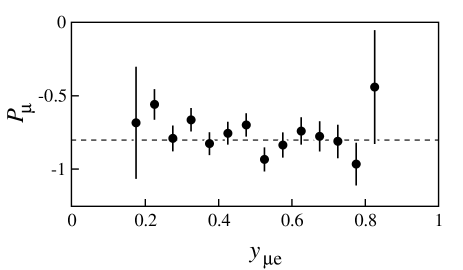
FIG. 7.: Beam polarization vs. the ratio of electron and muon energies from polarized $\mu$–e scattering. The dashed line represents the average value.

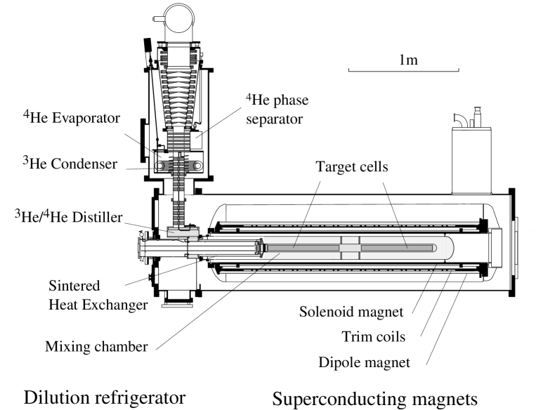
FIG. 8.: Cross section of the SMC polarized target.

3 The beam polarization

The beam polarization obtained from the $\mu$–e scattering experiment in 1993 is [74, 75]:

$$P_{\mu}=-0.779\pm 0.026\,(\mbox{stat.})\pm 0.017\,(\mbox{syst.})$$ (69)

for $E_{\mu}=187.9~{}\rm GeV$. The polarization measured by the muon decay method in 1993, $P_{\mu}=-0.803\pm 0.029\,(\mbox{stat.})\pm 0.020\,(\mbox{syst.})$, has been published earlier [9]. Both results are compatible. An alternative analysis with a larger data sample for the muon decay method is in progress and the systematic uncertainties of our previous analysis are being re-evaluated. The result of the $\mu$–e scattering Eq. (69) is used in this paper. For $E_{\mu}=100\,\rm GeV$ a value of $P_{\mu}=-0.82\pm 0.06$ was used for the analysis of the $A_{2}$ measurement. This is based on the measurement reported in Ref. [64]. Monte Carlo simulations of the muon beam [60] are consistent with these measurements of $P_{\mu}$ for both beam energies. We have evaluated the average polarization of our accepted event sample taking into account the energy dependence of the muon polarization. The polarization was calculated on an event-by-event basis using Eq. (64) and assuming a monoenergetic pion beam (Fig. 5).

D The polarized target

The polarized proton target uses the method of dynamic nuclear polarization (DNP) [76] and contains two oppositely polarized target cells exposed to the same muon beam (Fig. 8) [2]. The solid target material is butanol (CH₃(CH₂)₃OH) plus 5% water doped with paramagnetic EHBA-Cr(V) molecules. A superconducting magnet system [77] and a ³He –⁴He dilution refrigerator (DR) [78] provide the strong magnetic field and the low temperature required for high polarization, and allow for frequent inversion of the field and thus of the polarization vectors. Additional subsystems include a double microwave set-up needed for the DNP and a 10-channel NMR system to measure the spin polarization [79]. During data-taking, the nuclear spin axis is aligned either along or perpendicular to the beam direction in order to measure $A_{\parallel}$ or $A_{\perp}$, respectively.

The two target cells were each 60 cm long, cylindrical, polyester–epoxy mesh cartridges of 5 cm diameter, separated by a 30 cm gap. The target consisted of 1.8 mm butanol glass beads. The total amount of target material was 1.42 kg, with a packing fraction of 0.62 and a density of 0.985 g/cm³ at 77 K. The concentration of paramagnetic electron spins in the target material was $6.2\times 10^{19}$ spins/ml. In addition to butanol, the target cells contained other material, mostly the ³He –⁴He cooling liquid and the NMR coils for the polarization measurement (Table II).

In the 2.5 T field and at a temperature below 1 K, the electron spins are nearly 100% polarized. When their resonance line is saturated at a frequency just above or below the absorption spectrum centered around the frequency of $\nu_{e}\approx 69.3$ GHz at 2.5 T, negative and positive proton polarizations are obtained. This technique was applied to polarize the material in the two target cells in opposite directions. Modulation of the microwave frequencies with a 30 MHz amplitude and a 1 kHz rate increased the polarization build-up rate by 20% and resulted in a gain in maximum polarization of 6%. This method was originally developed to improve the polarization of a deuterated butanol target [80].

The DR [81] cools the target material to a temperature below 0.5 K while absorbing the microwave power applied for DNP. Once a high polarization is reached, the microwaves are turned off and the target material is cooled to 50 mK. At this temperature the proton spin-lattice relaxation time exceeds 1000 hours at 0.5 T. Under these ‘frozen spin’ conditions, the polarization is preserved during field rotation and during measurements with transverse spin. To avoid possible systematic errors, the proton polarizations were reversed by DNP once a week.

The superconducting magnet system [77, 78] consists of a solenoid with a longitudinal field of 2.5 T aligned with the beam axis, and a dipole providing a perpendicular ‘holding’ field of 0.5 T. The solenoid has a bore of 26.5 cm into which the DR with the target cells is inserted; this diameter corresponds to an opening angle of $\pm 65$ mrad with respect to the upstream end of the target. Sixteen correction coils allow the field to be adjusted to a relative homogeneity of $\pm 3.5\times 10^{-5}$ over the target volume. In addition, the trim coils were used to suppress the super-radiance effect [82], which can cause losses of the negative proton polarization while the field is being changed. The spin directions were reversed every five hours with relative polarization losses of less than $0.2\%$. This was accomplished by rotating the magnetic field vector of the superimposed solenoid and dipole fields, with a loss of data-taking time of only 10 minutes per rotation [83]. The dipole field was also used to hold the spin direction transverse to the beam for the measurement of $A_{\perp}$.

The proton polarization was measured with ten series-tuned Q-meter circuits with five NMR coils in each target cell [84, 85]. The polarization is proportional to the integrated NMR absorption signal which was determined from consecutively measured response functions of the circuit with and without the NMR signal. The latter was obtained by increasing the magnetic field, and thus shifting the proton NMR spectrum outside the integration window. The calibration constant was obtained from a measurement of the thermal equilibrium (TE) signals at 1 K, where the polarization is known from the Curie law $P_{\rm TE}={\rm tanh}\left({h\,\nu_{\rm p}}/{2\,k\,T}\right)\simeq 0.002553$; $T$ is the lattice temperature, $k$ the Boltzmann constant, and $\nu_{\rm p}$ is the proton Larmor frequency. The accuracy of the TE calibration signal contributed to the polarization error by $\Delta P/P=1.1\%$ [79]. The NMR signals were measured every minute during data-taking. The polarizations measured with the individual coils were averaged for each target cell and over the duration of one data taking run of typically 30 minutes. All measurements inside the same cell agreed to better than 3%. To detect a possible radial inhomogeneity, two of the five coils in the upstream target cell were at the same longitudinal position, but one was in the center and the other at a radius of 1 cm. No significant difference was found between the polarizations measured by these two coils.

TABLE II.: Quantities (in moles) of the various chemical elements in the target volume.

Element	Quantity	Element	Quantity	Element	Quantity
1H	185.70	F	0.24	Cu	00.36
3He	6.00	Na	0.17	O	22.70
4He	23.00	Cr	0.17	C	71.80
Ni	0.14

The characteristic polarization build-up time was two to three hours. However, the highest polarizations of $+0.93$ and $-0.94$ were achieved only after several days of DNP. The average polarization during the data-taking was 0.86, and the relative error in the average polarization of the target was estimated to be 3%.

TABLE III.: Detectors of the muon spectrometer.

Hodo-	Modules	Pitch	Size	Wire-	Modules	Pitch	Size	Dead
scope	$\times$Planes	(cm)	(cm)	chamber	$\times$Planes	(cm)	(cm)	zone(cm)
BHA-B	2$\times$8	0.4	8$\times$8	P0A-E	5$\times$8	0.1	$\oslash$ 14	—
V123	5$\times$1	—	various	PV1	1$\times$4	0.2	150$\times$94	—
H1	2	7.0	250$\times$130	PV2	1$\times$6	0.2	154$\times$100	$\oslash$ 8
H2 cal	4	28.0	560$\times$280	P123	3$\times$3	0.2	180$\times$80	$\oslash$ 13
H3	2	15.0	750$\times$340	W12	2$\times$8	2.0	220$\times$120	$\oslash$ 12
H4	1	15.0	996$\times$435	W45	6$\times$4	4.0	530$\times$260	$\oslash$ 13–25
H1’,3’,4’	1	1.4	50$\times$50	P45	5$\times$2	0.2	$\oslash$ 90	$\oslash$ 12
S1,2,4	1	—	various	ST67	4$\times$8	1.0	410$\times$410	$\oslash$ 16
H5	1$\times$2	various	19$\times$20	P67	4$\times$2	0.2	$\oslash$ 90	$\oslash$ 12
H6	1$\times$2	various	$\oslash$ 14	DT67	3$\times$4	5.2	500$\times$420	83$\times$83

E Muon spectrometer and event reconstruction

The spectrometer is similar to the set-ups used by the EMC [86] and the NMC (Fig. 2). Aging chambers were replaced and new ones added to improve the redundancy of the muon tracking and to extend the kinematic coverage to smaller $x$. A major new streamer tube detector ST67 was constructed to identify and measure scattered muon positions downstream of the absorber. Triggers were optimized for improved kinematic coverage, in particular in the region of small $x$.

1 Spectrometer layout

Three stages of the spectrometer can be distinguished: tracking of the incident muon, tracking and momentum measurement of the scattered muon, and muon identification. The beam tracking section upstream of the target is composed of two scintillator hodoscopes (BHA/BHB) and the P0B MWPC. A set of veto counters (V1.5, V3, V2.1 and V2) defines the beam spot size. Beam tracks are reconstructed with an angular resolution of 0.1 mrad and an efficiency better than 90% for intensities up to $5\times 10^{7}\,\mu/$spill.

The momentum of the scattered muon is measured with a conventional large-aperture dipole magnet (FSM) and a system of more than 100 planes of MWPC (Table III). The FSM is operated with bending powers of 2.3 and 4.4 Tm at 100 GeV and 190 GeV beam energies, respectively, corresponding to a horizontal beam deflection of 7 mrad. The angular resolution for scattered muons is 0.4 mrad. The large MWPC are complemented by smaller MWPC with a smaller wire pitch, to increase the redundancy and the resolution of the spectrometer in the high-rate environment at small scattering angles.

Scattered muons are identified by the observation of a track behind a 2 m thick iron absorber. The muon identification system consists of streamer tubes, MWPC and drift tubes. To cope with the high beam intensity, the streamer tubes were operated with voltages at which their pulse heights were close to the electronic threshold. Their efficiencies were thus very sensitive to the ambient pressure and temperature, and a high-voltage feedback system was developed to stabilize the average streamer pulse height within 1%.

2 Triggers

The read-out of the detectors was triggered by predefined coincidence patterns of hits in different planes of scintillation-counter hodoscopes. Three physics triggers provide a coverage of different $x$ and $Q^{2}$ ranges (Fig. 9). All triggers require that there is no hit in any of the beam-defining veto counters.

The large-angle trigger T1 requires a coincidence pattern of the hodoscopes H1, H3 and H4. This trigger has a good acceptance for scattering angles $\theta$ larger than 20 mrad. Target pointing of the scattered muon is also required. The acceptance decreases for smaller angles, but extends to $\theta\approx 3$ mrad. The small-angle trigger T2 uses the smaller hodoscopes H1’, H3’ and H4’. This trigger covers the range $5\,{\rm mrad}\leq\theta\leq 15$ mrad. It has a more limited $x$-range than T1. However, at a given $x$, T2 selects events with lower $Q^{2}$ than T1. A small-$x$ trigger T14 is provided by the S1, S2 and S4 counters which are placed close to the beam to cover scattering angles down to 3 mrad with good efficiency. The counters for T2 and T14 were located on the bending side of the spectrometer magnet. The acceptance of the triggers T1 and T14 extends down to $x\simeq 0.5\times 10^{-3}$ and thus is sensitive to elastic scattering of muons from atomic electrons, $x=m_{\rm e}/m_{\rm p}$ (Fig. 9). The trigger rate per SPS spill was about $200$ for T1, $50$ for T2 and $100$ for T14.

Other triggers include normalization and beam-halo triggers which were used for calibration, alignment, and efficiency calculations.

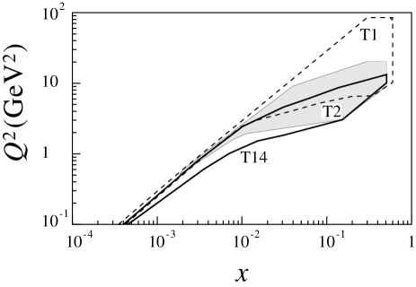
FIG. 9.: Kinematic ranges for triggers T1, T2 and T14 at 190 GeV.

TABLE IV.: Kinematic cuts applied for the $A_{\parallel}$ and $A_{\perp}$ analysis.

Kinematic	$A_{\parallel}$ analysis		$A_{\perp}$ analysis
variable	$E_{\mu}$ = 190 GeV		$E_{\mu}$ = 100 GeV
$\nu$	$\geq 15~{}\rm GeV$		$\geq 10~{}\rm GeV$
$y$	$\leq$ 0.9		$\leq$ 0.9
$p^{\prime}_{\mu}$	$\geq 19~{}\rm GeV$		$\geq 15~{}\rm GeV$
$\theta$	$\geq$ 9 mrad		$\geq$ 13 mrad
	Final Data Sample for $A_{\parallel}$ analysis		Final Data Sample for $A_{\perp}$ analysis
$x$ range	$0.003\leq x\leq 0.7$	$0.0008\leq x\leq 0.7$	$0.006\leq x\leq 0.6$	$0.0035\leq x\leq 0.6$
$Q^{2}$ range	$1\leq Q^{2}\leq 90$	$0.2\leq Q^{2}\leq 90$	$1\leq Q^{2}\leq 30$	$0.5\leq Q^{2}\leq 30$
Events	$4.5\times 10^{6}$	$6.0\times 10^{6}$	$8.8\times 10^{5}$	$9.6\times 10^{5}$

3 Event reconstruction

The track finding starts with the beam-track reconstruction. The momentum of the incident muons is computed from the hit pattern in the BMS hodoscopes. The beam track upstream of the target is found from the hits in the BHA and BHB hodoscopes and the P0B wire chamber. A coincidence is required between the hits in the BMS and those in the beam hodoscopes.

The reconstruction of the scattered muon tracks starts in the muon identification system behind the hadron absorber (ST67, DT67, P67). Tracks found in this system are extrapolated upstream and reconstructed in the MWPC and drift chambers between the absorber and the FSM (W45, P45, W12, P0E). The next step in the reconstruction is the track finding in the FSM chambers (P123, P0D), starting with the vertical coordinates which are fitted by straight lines. Horizontal coordinates matching the downstream tracks are searched for on circular trajectories inside the FSM. Because of the high track multiplicity in the FSM aperture, each extrapolation of a downstream track through the magnetic field is tested with a spline fit and the best track is retained. In the vertex chambers (PV12, P0C), hits are selected using the extrapolated track reconstructed in the magnet, and are fitted by a straight line. It is verified that the reconstructed muon track satisfies the trigger conditions.

The vertex position in the target is computed as the point of closest distance of approach between the beam and the scattered-muon tracks. Tracks are propagated through the magnetic field in the target using a Runge–Kutta method, taking into account energy loss and multiple scattering. In case of multiple beam tracks, the vertex with the best space-time correlation between the beam and the scattered-muon track is chosen. The vertex is reconstructed with resolutions of better than 30 mm and 0.3 mm along and perpendicular to the beam direction, respectively.

F Data-taking

The data presented in this paper were taken during 134 days of the 1993 CERN SPS fixed-target run. Most data were taken with longitudinal target polarization, at a beam energy of 190 GeV. For 22 days, data were taken with the target polarized transversely to the beam, at a beam energy of 100 GeV.

A total of 1.6$\times 10^{7}$ deep-inelastic-scattering events were reconstructed from the data with a longitudinally polarized target, using the three physics triggers T1, T2 and T14. The integrated muon flux was $1.7\times 10^{13}$.

With transverse target polarization, only T1 was used and 1.6 million events were reconstructed. The transverse target field was always in the same vertical direction and the spin direction was inverted by microwave reversal a total of 10 times. The integrated muon flux at 100 GeV was $0.2\times 10^{13}$.

G Event selection

Since the $A_{\parallel}$ and $A_{\perp}$ data were recorded at different beam energies, they cover different kinematic ranges and are subject to different kinematic cuts (Table IV). A cut at small $\nu$ rejects events with poor kinematic resolution, whereas a cut at high $y$ removes events with large radiative corrections. A cut on the momentum of the outgoing muon reduces the contamination by muons from $\pi$ and K production in the target and subsequent decay to a few $10^{-3}$. The cut on $\theta$ was only applied for the analysis with $Q^{2}\geq$1 GeV². It rejects events with poor vertex resolution.

Cuts were also applied to the beam phase space to ensure that the beam flux was the same for both target cells. Fiducial cuts on the target volume reject events from material outside the target cells (Fig. 10). Less than 10% of the raw data were discarded because of instabilities in the beam intensity, detector efficiencies, and target polarization. The size of the final data samples after all cuts is shown in Table IV.

IV DATA ANALYSIS

A Evaluation of cross section asymmetries

The two cross section asymmetries $A_{\parallel}$ and $A_{\perp}$ (Eq. (8)) are evaluated from counting rate asymmetries. To determine $A_{\parallel}$ the four measured counting rates from the upstream and downstream target cells with the two possible antiparallel target spin configurations are used. The quantity $A_{\rm T}=A_{\perp}\cos\phi$ is determined separately for the upstream and downstream target cells from the four counting rates into the upper and lower vertical halves of the spectrometer for the two transverse spin directions.

1 The $A_{\parallel}$ analysis

The number of muons $N_{\rm u}$ and $N_{\rm d}$ scattered in the upstream and downstream target cells, respectively, is given by

$$N_{\rm u}=n_{\rm u}\Phi\,a_{\rm u}\overline{\sigma}(1-fP_{\mu}P_{\rm u}A_{\parallel}),$$ (70)

$$N_{\rm d}=n_{\rm d}\Phi\,a_{\rm d}\overline{\sigma}(1-fP_{\mu}P_{\rm d}A_{\parallel}),$$ (71)

where $\Phi$ is the integrated beam flux, $P_{\rm u}$ and $P_{\rm d}$ are the polarizations in the two target cells, $n_{\rm u}$ and $n_{\rm d}$ the area densities of the target nucleons, and $a_{\rm u}$ and $a_{\rm d}$ are the corresponding spectrometer acceptances. The dilution factor $f$ accounts for the fact that only a fraction of the target nucleons is polarized (Section IV C). The flux $\Phi$ and the spin-independent cross section $\overline{\sigma}$ cancel in the evaluation of the raw counting-rate asymmetries, $A_{\rm RAW}$ and $A_{\rm RAW}^{\prime}$, obtained before and after target polarization reversal:

$$A_{\rm RAW}=\frac{N_{\rm u}-N_{\rm d}}{N_{\rm u}+N_{\rm d}},\hskip 42.67912ptA_{\rm RAW}^{\prime}=\frac{N_{\rm d}^{\prime}-N_{\rm u}^{\prime}}{N_{\rm d}^{\prime}+N_{\rm u}^{\prime}}.$$ (72)

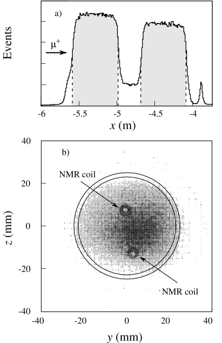
FIG. 10.: Vertex distributions of scattered muons after kinematic cuts: (a) along the beam direction and (b) in the plane perpendicular to the target axis, at the location of one of the NMR coils. In (a), the dashed lines indicate the fiducial cuts on the target volume which coincide with the entry and exit windows of the target cells; most events outside the shaded region originate from interactions with the ³He –⁴He cooling liquid. The small peak at $x\approx-3.9$ m arises from scattering in the exit window of the target cryostat. In (b), the outer circle indicates the wall of the target cells, and the inner circle shows the radial cut applied. Scattering from the tubular NMR coils is clearly visible.

Provided that the ratio of acceptances is the same before and after polarization reversal, i.e. $a_{\rm u}/a_{\rm d}=a^{\prime}_{\rm u}/a^{\prime}_{\rm d}$, and since $n_{\rm u}/n_{\rm d}$ is constant, the acceptances $a$ and the densities $n$ cancel in the average of the raw asymmetries, so that

$$A_{\parallel}=-\frac{1}{fP_{\mu}P_{\rm t}}\left[\frac{A_{\rm RAW}+A_{\rm RAW}^{\prime}}{2}\right].$$ (73)

If $a_{\rm u}/a_{\rm d}\neq a_{\rm u}^{\prime}/a_{\rm d}^{\prime}$ a ‘false’ asymmetry ensues,

$$A_{\rm false}=-\frac{1}{2fDP_{\mu}P_{\rm t}}\left[\,\frac{r-1}{r+1}-\frac{r^{\prime}-1}{r^{\prime}+1}\right].$$ (74)

The virtual photon-proton asymmetry $A_{1}\simeq A_{\parallel}/D$ (Eq. (17)) is thus given by:

$$A_{1}=-\frac{1}{fDP_{\mu}P_{\rm t}}\left[\frac{A_{\rm RAW}+A_{\rm RAW}^{\prime}}{2}\right]-A_{\rm false}.$$ (75)

In these expressions, $D$ is the depolarization factor (Eq. (15)), $r=n_{\rm u}a_{\rm u}/n_{\rm d}a_{\rm d}$, $r^{\prime}=n_{\rm u}a_{\rm u}^{\prime}/n_{\rm d}a_{\rm d}^{\prime}$ and $P_{\rm t}$ is the weighted average of the target cell polarizations,

$$2P_{\rm t}=\frac{\sum|P_{\rm u}|N_{\rm u}+\sum|P_{\rm d}|N_{\rm d}}{\sum N_{\rm u}+\sum N_{\rm d}}+\frac{\sum|P_{\rm u}^{\prime}|N_{\rm u}^{\prime}+\sum|P_{\rm d}^{\prime}|N_{\rm d}^{\prime}}{\sum N_{\rm u}^{\prime}+\sum N_{\rm d}^{\prime}}.$$ (76)

Equation (75) provides an unbiased estimate of the cross section asymmetry for large numbers of events. To avoid possible biases for the number of events involved, a maximum likelihood technique was developed which allows a common analysis of all events in each $x$-bin. In this method, $A_{\parallel}/D$ is computed from the event weights $w=fDP_{\mu}$ using the expression

$$A_{1}= - \frac{1}{2P_{\rm t}}\left[{\left(\frac{\sum w_{\rm u}-\sum w_{\rm d}}{\sum w_{\rm u}^{2}+\sum w_{\rm d}^{2}}\right)+\left(\frac{\sum w_{\rm d}-\sum w_{\rm u}}{\sum w_{\rm d}^{2}+\sum w_{\rm u}^{2}}\right)^{\prime}}~{}\right]$$ (77)

$$- A_{\rm false}.$$ (78)

As explained in Section IV C, in the actual analysis we use a weight $w=f^{\prime}DP_{\mu}$. A Monte Carlo simulation confirmed that this method does not introduce any biases.

2 The $A_{\perp}$ analysis

A similar formalism applies to the measurement of the transverse asymmetry $A_{\perp}$, where the event yields are given by $N(\phi)=n\Phi a\overline{\sigma}(1-fP_{\mu}P_{\rm T}\cos\phi A_{\perp})$. Here, $A_{\perp}$ is obtained for each target cell separately from $[N(\phi)-N(\phi-\pi)]/[N(\phi)+N(\phi-\pi)]$ and $A_{\perp}/d$ becomes

$$\frac{A_{\perp}}{d} = \frac{-1}{2P_{\mu}\langle P_{\rm t}\rangle}\left[\left(\frac{\sum fd~{}{\cos\phi}}{\sum(fd~{}\cos\phi)^{2}}\right)+\left(\frac{\sum fd{\cos\phi}}{\sum(fd\cos\phi)^{2}}\right)^{\prime}\right]$$ (79)

$$- A_{\rm false},$$ (80)

where $\langle P_{\rm t}\rangle$ is the average target polarization before and after reversal in absolute value. To obtain the same statistical accuracy for $A_{\perp}/d$ and for $A_{\parallel}/D$ more data are required for $A_{\perp}/d$ due to its dependence on $\cos\phi$, and also to a lesser extent to the fact that $d<D$.

B Radiative corrections

QED radiative corrections are applied to convert the measured asymmetries (78) and (80) to one-photon exchange asymmetries. These corrections are calculated using:

$$\overline{\sigma}^{\rm T} = v\overline{\sigma}^{1\gamma}+\overline{\sigma}_{\rm tail},$$ (81)

$$\Delta\sigma^{\rm T} = v\Delta\sigma^{1\gamma}+\Delta\sigma_{\rm tail},$$ (82)

where $\overline{\sigma}^{\rm T}$ is the total, i.e. measured, spin-independent cross-section, $\overline{\sigma}^{1\gamma}$ is the corresponding one-photon exchange cross section, and $\overline{\sigma}_{\rm tail}$ is the contribution to $\overline{\sigma}^{\rm T}$ from the elastic tail and the inelastic continuum. The corresponding differences of the cross sections for antiparallel and parallel orientations of lepton and target spins are denoted by $\Delta\sigma$. The factor $v$ accounts for vacuum polarization and also includes contributions from the inelastic tail close in $x$. The decomposition in Eq. 81 depends on the fraction of the inelastic tail included in $v$ and is therefore to some extend ambiguous. Due to a cancelation of the different contributions, $v$ is close to unity. Using the program TERAD [88] we find $0.98<v<1.03$ in the kinematic range of our data. For simplicity we set $v$ to unity in our analysis and attribute all corrections to $\sigma_{\rm tail}$ [87].

Neglecting $A_{2}$ and thus implying $A_{1}=\Delta\sigma/(2D\sigma)$, the radiative corrections to the one-photon asymmetry, $A_{1}^{1\gamma}$, can be written as

$$A_{1}^{\rm T}=\rho(A_{1}^{1\gamma}+A_{1}^{\rm rc}),$$ (83)

with $\rho=v\,\overline{\sigma}^{1\gamma}/\overline{\sigma}^{\rm T}$ and $A_{1}^{\rm rc}=\Delta{\sigma}_{\rm tail}/2vD\overline{\sigma}^{1\gamma}$.

The ratio $\overline{\sigma}^{1\gamma}/\overline{\sigma}^{\rm T}$ and the correction $A_{1}^{\rm rc}$ are evaluated using the program POLRAD [89, 90]. The asymmetry $A_{1}^{\rm p}(x)$ required as input is taken from Refs. [2, 9, 6] and the contribution from $A_{2}^{\rm p}$ is neglected. The uncertainty in $A_{1}^{\rm rc}$ is estimated by varying the input values of $A_{1}^{\rm p}$ within the errors. The factor $\rho$ and the additive correction $A_{1}^{\rm rc}$ are shown in Table V at the average $Q^{2}$ of each $x$-bin.

We have incorporated $\rho$ into the evaluation of the dilution factor, $f^{\prime}=\rho f$, on an event-by-event basis. Using the weight $w=f^{\prime}DP_{\mu}$ we directly obtain $A_{1}^{\rm T}/\rho$ on the left-hand side of Eq. 78 and thus $A_{1}^{1\gamma}$ (Eq. (83)).

The radiative corrections to the transverse asymmetry $A_{\perp}^{\rm T}$ are evaluated as above, however assuming that $g_{2}=g_{2}^{\rm WW}$ [55]. The additive correction is much smaller than the statistical error and has been neglected.

TABLE V.: The virtual photon-proton asymmetry $A_{1}^{\rm p}$ for $Q^{2}>1~{}{\rm GeV}^{2}$ (top) and $Q^{2}>0.2~{}{\rm GeV}^{2}$ (bottom). In the last column, the first error is statistical and the second is systematic. $\langle A_{\rm RAW}\rangle$ is the straight average of $A_{\rm RAW}$ and $A_{\rm RAW}^{\prime}$ in Eq. (73). The values for $A_{1}^{\rm p}$ have been corrected for radiative effects as described in Section IV B.

$x$ range	$\langle x\rangle$	$\langle Q^{2}\rangle$	$\langle{P_{\mu}}\rangle$	$\langle y\rangle$	$\langle D\rangle$	$\langle f\rangle$	$\langle\rho\rangle$	$\langle A_{\rm RAW}\rangle$	$A_{1}^{\rm rc}$	$A_{1}^{\rm p}$
		$({\rm GeV^{2}})$
.003–.006	.005	1.320	-.79	.791	.80	.070	1.50	.004	$.007$	$.083$$\pm$$.041$$\pm$$.006$
.006–.010	.008	2.068	-.78	.748	.76	.081	1.39	.003	$.008$	$.044$$\pm$$.037$$\pm$$.004$
.010–.020	.014	3.562	-.78	.704	.72	.090	1.30	.003	$.010$	$.061$$\pm$$.032$$\pm$$.004$
.020–.030	.025	5.733	-.78	.660	.68	.096	1.24	.003	$.012$	$.068$$\pm$$.044$$\pm$$.005$
.030–.040	.035	7.797	-.78	.634	.66	.099	1.21	.002	$.015$	$.041$$\pm$$.052$$\pm$$.003$
.040–.060	.049	10.445	-.78	.603	.64	.102	1.18	.006	$.017$	$.104$$\pm$$.045$$\pm$$.007$
.060–.100	.077	15.011	-.78	.551	.60	.106	1.14	.009	$.020$	$.180$$\pm$$.045$$\pm$$.013$
.100–.150	.122	21.411	-.78	.498	.55	.112	1.10	.013	$.022$	$.289$$\pm$$.058$$\pm$$.019$
.150–.200	.173	27.799	-.79	.456	.51	.118	1.08	.012	$.022$	$.276$$\pm$$.080$$\pm$$.019$
.200–.300	.242	35.542	-.79	.417	.47	.127	1.05	.010	$.019$	$.246$$\pm$$.082$$\pm$$.017$
.300–.400	.342	45.453	-.78	.377	.43	.139	1.02	.021	$.010$	$.499$$\pm$$.132$$\pm$$.036$
.400–.700	.482	57.089	-.78	.337	.39	.156	0.99	.022	$\!\!\!\!-.006$	$.527$$\pm$$.174$$\pm$$.041$
.0008–.0012	.001	0.285	-.78	.808	.85	.044	1.74	$\!\!\!\!-.001$	$.002$	$\!\!\!\!-.032$$\pm$.077$\pm$.004
.0012–.002	.002	0.445	-.78	.794	.83	.054	1.65	.002	$.003$	.085 $\pm$.055$\pm$.007
.002–.003	.003	0.686	-.78	.781	.80	.062	1.56	.001	$.004$	.031 $\pm$.054$\pm$.004
.003–.006	.004	1.193	-.78	.763	.77	.073	1.46	.003	$.006$	.059 $\pm$.034$\pm$.005
.006–.010	.008	2.038	-.78	.738	.75	.082	1.38	.003	$.008$	.050 $\pm$.036$\pm$.004

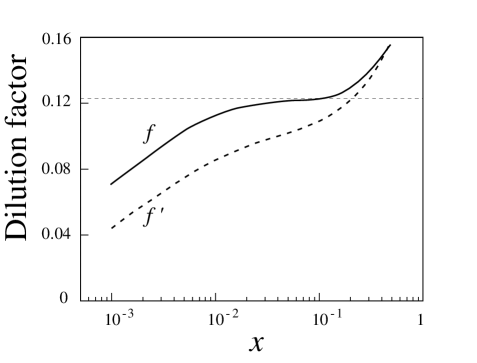
FIG. 11.: The dilution factor $f$ (solid line) and the effective dilution factor $f{{}^{\prime}}=\rho f$ (dashed line) as a function of $x$.

C Dilution factor

In addition to butanol, the target cells contain the NMR coils and the ³He –⁴He coolant mixture. The composition in terms of chemical elements is summarized in Table II. The dilution factor $f$ can be expressed in terms of the number $n_{A}$ of nuclei with mass number $A$ and the corresponding total spin-independent cross sections $\overline{\sigma}^{\rm T}_{A}$ per nucleon for all the elements involved:

$$f=\frac{n_{\rm H}\cdot\overline{\sigma}^{\rm T}_{\rm H}}{\sum_{A}n_{A}\cdot\overline{\sigma}^{\rm T}_{A}}.$$ (84)

The total cross section ratios $\overline{\sigma}_{A}^{\rm T}/\overline{\sigma}_{\rm H}^{\rm T}$ for D, He, C and Ca are obtained from the structure function ratios $F_{2}^{\rm n}/F_{2}^{\rm p}$ [91] and $F_{2}^{A}/F_{2}^{\rm d}$ [92]. The original procedure leading from the measured cross section rations $\overline{\sigma}^{\rm T}_{A}/\overline{\sigma}^{\rm T}_{H}$ to the published structure function ratios was inverted step by step involving the isoscalarity corrections and radiative corrections (TERAD). For unmeasured nuclei the cross section ratios are obtained in the same way from a parameterization of $F_{2}^{A}(x)/F_{2}^{\rm d}(x)$ as a function of $A$ [93, 94, 95].

The dilution factor also accounts for the contamination from material outside the finite target cells due to vertex resolution. This correction is applied as a function of the scattering angle, and the largest contamination occurs for the angles between 2 and 9 mrad, which results in a reduction of the dilution factor by about 6%. The correction needed because of the NMR coils (Fig. 10) is convoluted with the distribution of the beam intensity profile.

In the actual evaluation of Eqs. (78) and (80) we use an effective dilution factor $f^{\prime}$ (Fig. 11):

$$f^{\prime}=\rho f,$$ (85)

as discussed in Section IV B. The present procedure guarantees a proper calculation of the statistical error in the asymmetry, in contrast to our previous analysis [9, 10, 11, 12] where all radiative effects were included as an additive radiative correction. We find an increase in the statistical error by a factor $1/\rho$ which reaches 5 at small-$x$ (Table V). However, the central values of the asymmetries remain unaffected by the change in the radiative correction procedure [87].

The dilution factor is shown in Fig. 11 where it is compared to the ‘naive’ expectation for a mixture of 62% butanol, ($\rm CH_{3}(CH_{2})_{3}OH$), and 38% helium by volume, $f\simeq 0.123$. The rise of $f$ at $x>0.3$ is due to the decrease of the ratio $F_{2}^{\rm n}/F_{2}^{\rm p}$, whereas the drop in the low $x$-range is due to the larger contribution of radiative processes from elements with mass number much larger than hydrogen.

D The longitudinal cross section asymmetry

1 Results for $A_{1}^{\rm p}$

The virtual photon asymmetry $A_{1}^{\rm p}$ is calculated from Eqs. (78), (83) and (85) under the assumption that $A_{\rm false}=0$. The uncertainty introduced by this assumption is estimated using Eq. (74).

The results for $A_{1}^{\rm p}$ for $Q^{2}\geq 1\,{\rm GeV}^{2}$ are shown in Table V and in Fig. 12. The kinematic quantities in Table V are mean values within the bins calculated with the weighting factor $(f^{\prime}DP_{\mu})^{2}$. In addition to the results given in Ref. [9], we include here data obtained with the T14 trigger (Section III E 2). In Table V and in Fig. 12, we also show data in the kinematic range $0.2~{}\,\rm GeV^{2}\leq Q^{2}\leq 1~{}\,\rm GeV^{2}$, $0.0008\leq x\leq 0.003$. These data are not used to evaluate $g_{1}^{\rm p}$ or its first moment.

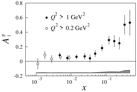
FIG. 12.: The virtual photon asymmetry $A_{1}^{\rm p}$ as a function of $x$. The error bars show statistical errors only; the systematic errors are indicated by the shaded area.

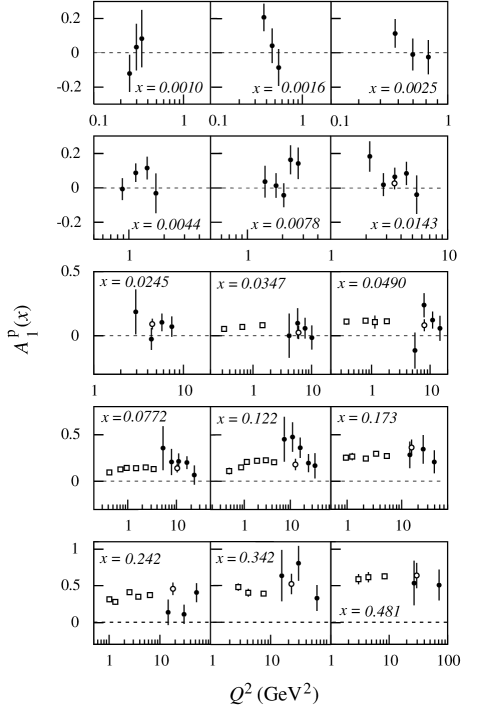
FIG. 13.: The virtual photon-proton asymmetry $A_{1}^{\rm p}$ as a function of $Q^{2}$, for constant values of $x$. The closed circles are data from this experiment. The data of the EMC and E143 experiments are also shown as open circles and squares, respectively.

The sources of systematic errors in $A_{1}^{\rm p}$ are time-dependence instabilities of the acceptance ratios $r$ and $r^{\prime}$, uncertainties in the beam and target polarizations, in the effective dilution factor $f^{\prime}$, the radiative corrections, and in $R=\sigma_{L}/\sigma_{T}$, and the neglect of $A_{2}$. The individual errors (Table VI) are combined in quadrature to obtain the total systematic error (Table V).

TABLE VI.: Contributions to the systematic errors at the average $Q^{2}$ of the $x$-bin.

$\langle x\rangle$	$\Delta A_{\rm false}$	$\Delta P_{\rm t}$	$\Delta P_{\mu}$	${\Delta f^{\prime}}$	$\Delta\rm rc$	$\Delta A_{2}$	$\Delta R$
0.005	0.0021	0.0025	0.0033	0.0016	0.0012	0.0006	0.0027
0.008	0.0019	0.0013	0.0017	0.0008	0.0012	0.0007	0.0012
0.014	0.0019	0.0018	0.0024	0.0011	0.0011	0.0009	0.0021
0.025	0.0018	0.0020	0.0027	0.0013	0.0010	0.0002	0.0031
0.035	0.0018	0.0012	0.0016	0.0008	0.0010	0.0003	0.0016
0.049	0.0018	0.0031	0.0041	0.0020	0.0009	0.0003	0.0040
0.077	0.0019	0.0054	0.0071	0.0035	0.0009	0.0004	0.0080
0.122	0.0019	0.0087	0.0114	0.0058	0.0010	0.0005	0.0112
0.173	0.0020	0.0083	0.0109	0.0056	0.0010	0.0005	0.0110
0.242	0.0020	0.0074	0.0097	0.0051	0.0009	0.0022	0.0105
0.342	0.0020	0.0150	0.0197	0.0107	0.0007	0.0025	0.0236
0.482	0.0020	0.0158	0.0208	0.0117	0.0008	0.0030	0.0293
0.0011	0.0032	0.0010	0.0013	0.0011	0.0009	0.0005	0.0017
0.0016	0.0027	0.0025	0.0034	0.0026	0.0010	0.0008	0.0035
0.0025	0.0024	0.0009	0.0012	0.0009	0.0011	0.0011	0.0012
0.0044	0.0021	0.0018	0.0024	0.0014	0.0012	0.0007	0.0023
0.0078	0.0020	0.0015	0.0020	0.0010	0.0012	0.0008	0.0015

TABLE VII.: The virtual photon-proton asymmetry $A_{1}^{\rm p}$ as a function of $x$ and $Q^{2}$. Only statistical errors are shown.

$\langle x\rangle$	$\langle Q^{2}\rangle$	$A_{1}^{\rm p}$	$\langle x\rangle$	$\langle Q^{2}\rangle$	$A_{1}^{\rm p}$
	$({\rm GeV^{2}})$			$({\rm GeV^{2}})$
0.0009	0.25	$\!\!-0.122\pm$ 0.110	0.0345	7.77	0.058 $\pm$ 0.082
0.0010	0.30	0.033 $\pm$ 0.137	0.0359	10.15	$\!\!-0.012\pm$ 0.095
0.0011	0.34	0.082 $\pm$ 0.169	0.0474	2.94	$\!\!-1.114\pm$ 0.589
0.0014	0.38	0.209 $\pm$ 0.081	0.0473	5.49	$\!\!-0.117\pm$ 0.142
0.0017	0.46	0.042 $\pm$ 0.102	0.0478	7.83	0.241 $\pm$ 0.094
0.0018	0.55	$\!\!-0.086\pm$ 0.109	0.0484	10.96	0.123 $\pm$ 0.068
0.0023	0.58	0.114 $\pm$ 0.085	0.0527	14.73	0.058 $\pm$ 0.098
0.0025	0.70	$\!\!-0.009\pm$ 0.094	0.0738	5.33	0.359 $\pm$ 0.239
0.0028	0.82	$\!\!-0.025\pm$ 0.102	0.0744	7.88	0.212 $\pm$ 0.142
0.0036	0.88	$\!\!-0.006\pm$ 0.065	0.0751	11.09	0.214 $\pm$ 0.088
0.0043	1.14	0.089 $\pm$ 0.054	0.0762	16.32	0.203 $\pm$ 0.068
0.0051	1.43	0.119 $\pm$ 0.067	0.0855	23.04	0.066 $\pm$ 0.105
0.0057	1.70	$\!\!-0.033\pm$ 0.118	0.1193	7.36	0.456 $\pm$ 0.242
0.0070	1.42	0.037 $\pm$ 0.094	0.1199	11.16	0.480 $\pm$ 0.159
0.0072	1.76	0.014 $\pm$ 0.073	0.1204	16.47	0.364 $\pm$ 0.110
0.0077	2.04	$\!\!-0.045\pm$ 0.071	0.1208	24.84	0.199 $\pm$ 0.098
0.0085	2.34	0.166 $\pm$ 0.085	0.1293	34.28	0.172 $\pm$ 0.137
0.0092	2.72	0.145 $\pm$ 0.093	0.1713	14.15	0.288 $\pm$ 0.143
0.0122	2.15	0.184 $\pm$ 0.090	0.1717	24.92	0.349 $\pm$ 0.156
0.0125	2.82	0.020 $\pm$ 0.067	0.1742	39.54	0.212 $\pm$ 0.123
0.0141	3.52	0.066 $\pm$ 0.053	0.2384	14.53	0.139 $\pm$ 0.176
0.0165	4.43	0.085 $\pm$ 0.069	0.2396	29.71	0.110 $\pm$ 0.132
0.0184	5.43	$\!\!-0.042\pm$ 0.113	0.2462	52.76	0.413 $\pm$ 0.131
0.0235	2.95	0.189 $\pm$ 0.176	0.3392	15.29	0.644 $\pm$ 0.354
0.0236	4.38	$\!\!-0.026\pm$ 0.086	0.3408	29.82	0.814 $\pm$ 0.241
0.0242	5.75	0.107 $\pm$ 0.070	0.3432	61.49	0.333 $\pm$ 0.179
0.0263	7.42	0.072 $\pm$ 0.080	0.4747	26.74	0.541 $\pm$ 0.306
0.0339	4.14	0.003 $\pm$ 0.174	0.4858	71.58	0.518 $\pm$ 0.213
0.0341	5.81	0.097 $\pm$ 0.119

Table VII and Fig. 13 show $A_{1}^{\rm p}$ as a function of $Q^{2}$ and $x$, including the data with $Q^{2}\leq 1~{}\,\rm GeV^{2}$. In Figure 13, a small correction is applied to the data to display them at the same average $x$ in each bin. A study of the $Q^{2}$ dependence which includes the SMC data [9, 12] was first made by the E143 collaboration for $0.03\leq x\leq 0.6$ and $Q^{2}>0.3$ $\rm GeV^{2}$, and showed no significant $Q^{2}$ dependence for $Q^{2}>1~{}\,\rm GeV^{2}$ [96]. We study here the $Q^{2}$ dependence for $0.003\leq x\leq 0.03$. A parametrization $A_{1}=a+b\log Q^{2}$ is fitted to the data and $b$ is found to be consistent with zero for all $x$ in this range. When fitting a parametrization $a^{\prime}+c/Q^{2}$ to account for possible higher twist effects, we again find no significant $Q^{2}$ dependence.

2 Comparison with earlier experiments

In Figure 14, we compare our results for $A_{1}^{\rm p}$ with data from earlier experiments [1, 2, 6, 96]. Good agreement is observed in the kinematic region of overlap. A consistency test between the SLAC E80/E130, EMC, SLAC E143 and SMC data yields a $\chi^{2}=11.4$ for 16 degrees of freedom. Since the average $Q^{2}$ of SMC and E143 differ by a factor of seven, the good agreement confirms the earlier conclusion that no $Q^{2}$ dependence is observed within the present accuracy of the data.

TABLE VIII.: Results on the asymmetry $A_{2}^{\rm p}$. Only statistical errors are given. The $A_{2}^{\rm p}$ values are the average values from the two target cells.

$x$ range	$\langle x\rangle$	$\langle Q^{2}\rangle$ (GeV2)	$A_{2}^{\rm p}$
0.006 – 0.015	0.010	1.4	$~{}~{}0.002\pm 0.109$
0.015 – 0.050	0.026	2.7	$~{}~{}0.041\pm 0.076$
0.050 – 0.150	0.080	5.8	$~{}~{}0.017\pm 0.099$
0.150 – 0.600	0.226	11.8	$~{}~{}0.149\pm 0.161$
0.0035 – 0.006	0.005	0.7	$-0.066\pm 0.167$
0.006 – 0.015	0.01	1.3	$~{}~{}0.086\pm 0.097$

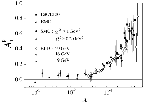
FIG. 14.: The virtual photon-proton asymmetry $A_{1}^{\rm p}$ as a function of $x$ from this experiment, compared with data from the EMC and the SLAC E80, E130, and E143 experiments. For E143, the structure function ratio $g_{1}^{\rm p}/F_{1}^{\rm p}$ is shown instead of $A_{1}^{\rm p}$. The errors are statistical only.

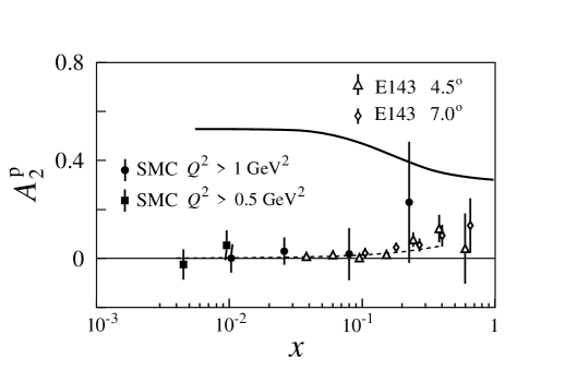
FIG. 15.: Results for the asymmetry $A_{2}^{\rm p}(x)$ extrapolated to $Q^{2}_{0}=5\,\rm GeV^{2}$ assuming $\sqrt{Q^{2}}A_{2}^{\rm p}$ scales [10]. The solid and dashed curves show the limit $|A_{2}|<\sqrt{R}$ and the prediction corresponding to $\bar{g}_{2}=0$, respectively. Also shown are data from the E143 experiment [41] extrapolated to the same $Q^{2}_{0}$ assuming that ${\sqrt{Q^{2}}A_{2}}$ scales. The errors are statistical only.

E The transverse cross section asymmetry

1 Results for $A_{2}^{\rm p}$

The asymmetry $A_{2}^{\rm p}$ is obtained from our measurements of $A_{\perp}^{\rm p}$ [10] and of $A_{\parallel}^{\rm p}$ [1, 2, 9], using Eq. (19). It is seen from Eq. (10), that $A_{2}$ has an explicit $1/\sqrt{Q^{2}}$ dependence and hence it is convenient to evaluate $\sqrt{Q^{2}}A_{2}^{\rm p}$ assuming that it is independent of $Q^{2}$ in Eq. (80). Our results do not depend on this assumption [97].

The results for the asymmetry $A_{2}^{\rm p}$ are shown in Table VIII and in Fig. 15. They are significantly smaller than the positivity limit $|A_{2}|\leq\sqrt{R}$ and are consistent with $A_{2}^{\rm p}=0$ and with the assumption that $g_{2}=g_{2}^{\rm WW}$, i.e. $\bar{g}_{2}=0$. Also shown in Fig. 15 are the E143 data [41]. They confirm our results, with better statistical accuracy, for $x>0.03$.

The main systematic uncertainties are due to the parametrizations of $A_{\parallel}^{\rm p}/D$ and $R$. The effects due to time variations of the acceptance are negligible as expected, since the results depend on the ratio of acceptances for muons scattered into the top and the bottom halves of the spectrometer, which should be affected in the same way by typical variations of chamber efficiencies. The errors from the dilution factor and the beam and target polarizations are also very small. The total systematic error on $A_{2}^{\rm p}$ is at least one order of magnitude smaller than the statistical error at all values of $x$.

TABLE IX.: Results for the spin-dependent structure function $g_{1}^{\rm p}$. The first error is statistical and the second is systematic. The third error in the last column is the uncertainty associated with the QCD evolution.

$x$-range	$\langle x\rangle$	$\langle Q^{2}({\rm GeV^{2}})\rangle$	$g_{1}^{\rm p}(x,Q^{2})$	$g_{1}^{\rm p}(x,Q^{2}_{0}=10\,{\rm GeV^{2}})$
$0.003$–$0.006$	$0.005$	$1.3$	$1.97$$\pm$$0.97$$\pm$$0.15$	$2.37$$\pm$$0.97$$\pm$$0.15$$\pm$$0.66$
$0.006$–$0.010$	$0.008$	$2.1$	$0.73$$\pm$$0.61$$\pm$$0.06$	$1.03$$\pm$$0.61$$\pm$$0.06$$\pm$$0.17$
$0.010$–$0.020$	$0.014$	$3.6$	$0.63$$\pm$$0.33$$\pm$$0.05$	$0.79$$\pm$$0.33$$\pm$$0.05$$\pm$$0.04$
$0.020$–$0.030$	$0.025$	$5.7$	$0.45$$\pm$$0.29$$\pm$$0.03$	$0.51$$\pm$$0.29$$\pm$$0.03$$\pm$$0.02$
$0.030$–$0.040$	$0.035$	$7.8$	$0.20$$\pm$$0.26$$\pm$$0.02$	$0.22$$\pm$$0.26$$\pm$$0.02$$\pm$$0.01$
$0.040$–$0.060$	$0.049$	$10.4$	$0.38$$\pm$$0.17$$\pm$$0.02$	$0.37$$\pm$$0.17$$\pm$$0.02$$\pm$$0.00$
$0.060$–$0.100$	$0.077$	$15.0$	$0.42$$\pm$$0.10$$\pm$$0.02$	$0.40$$\pm$$0.10$$\pm$$0.02$$\pm$$0.01$
$0.100$–$0.150$	$0.122$	$21.4$	$0.41$$\pm$$0.08$$\pm$$0.03$	$0.39$$\pm$$0.08$$\pm$$0.02$$\pm$$0.01$
$0.150$–$0.200$	$0.173$	$27.8$	$0.26$$\pm$$0.08$$\pm$$0.02$	$0.25$$\pm$$0.08$$\pm$$0.02$$\pm$$0.01$
$0.200$–$0.300$	$0.242$	$35.5$	$0.15$$\pm$$0.05$$\pm$$0.01$	$0.15$$\pm$$0.05$$\pm$$0.01$$\pm$$0.01$
$0.300$–$0.400$	$0.342$	$45.5$	$0.15$$\pm$$0.04$$\pm$$0.01$	$0.17$$\pm$$0.04$$\pm$$0.01$$\pm$$0.00$
$0.400$–$0.700$	$0.482$	$57.1$	$0.06$$\pm$$0.02$$\pm$$0.00$	$0.08$$\pm$$0.02$$\pm$$0.00$$\pm$$0.00$

V RESULTS FOR $g_{1}^{\rm p}$ AND ITS FIRST MOMENT

A Evaluation of $g_{1}^{\rm p}(x,Q^{2})$

The spin-dependent structure function $g_{1}^{\rm p}$ is evaluated from the virtual photon-proton asymmetry $A_{1}^{\rm p}$ using Eqs.(17) and (18). This analysis is restricted to $Q^{2}>1\,\rm GeV^{2}$. For $F_{2}$, we use the parametrization of Ref. [98] and for $R$ the parametrization of Ref. [99]. The parametrization of $R$ is based on data for $x>0.01$ only and therefore must be extrapolated to cover smaller values of $x$. However, the structure function $g_{1}$ at the average $Q^{2}$ of the measurement is nearly independent of $R$ due to a partial cancelation between the $R$ dependence of $D$, of $F_{2}$, and of the explicit term $(1+R(x,Q^{2}))$. The results for $g_{1}^{\rm p}$ are shown in Table IX and, together with our deuteron data [13], in Fig. 16.

TABLE X.: Parameters of the polarized parton distributions at $Q^{2}_{\mathrm{ref}}=1$ GeV², obtained from the QCD fit discussed in the text.

	$a$	$\alpha$	$\beta$	$\eta$
$\Delta q^{\rm NS}$	$~{}~{}25.4\pm 39.1$	$-0.67\pm 0.25$	$2.12\pm 0.28$	proton: $1.087\pm 0.006$ (fixed)
				deuteron: $0.145\pm 0.002$ (fixed)
$\Delta\Sigma$	$-1.30\pm 0.16$	$0.71\pm 0.33$	$1.56\pm 1.00$	$0.40\pm 0.04$
$\Delta g$	$a_{\Delta\Sigma}$	$-0.70\pm 0.27$	$4$ (fixed)	$0.98\pm 0.61$

B Evolution of $g_{1}^{\rm p}$ to a fixed $Q^{2}_{0}$

To evaluate the first moment $\Gamma_{1}^{\rm p}=\int_{0}^{1}g_{1}^{\rm p}{\rm d}x$, the measured $g_{1}(x,Q^{2})$ must be evolved to a common $Q^{2}_{0}$ for all $x$. In previous analyses, $g_{1}(x,Q_{0}^{2})$ was obtained assuming $A_{1}\simeq g_{1}/F_{1}$ to be independent of $Q^{2}$. This assumption is consistent with the data. However, perturbative QCD predicts the $Q^{2}$ dependences of $g_{1}$ and $F_{1}$ to differ by a considerable amount at small-$x$. The evolution of $g_{1}/F_{1}$ is poorly constrained by the data in this region, where the data cover a very narrow $Q^{2}$ range. Recent experimental and theoretical progress allows us to perform a QCD analysis of polarized structure functions in next–to–leading order NLO, and therefore a realistic evolution of $g_{1}$ can be obtained. Three groups have published such analyses [31, 100, 101]. They all use the splitting and coefficient functions calculated to NLO in the $\overline{\rm MS}$ scheme [23, 24, 25], but the choices made for the reference scales $Q_{\rm ref}^{2}$ at which the polarized parton distributions are parametrized and the forms of the parametrization are different. Also the selections of data sets used for the fits differ. In Ref. [31] the splitting and coefficient functions are transformed from the $\overline{\rm MS}$ scheme to different factorization schemes before the fits are performed. We shall refer to the results obtained in the Adler–Bardeen scheme.

FIG. 16.: The structure functions $g_{1}^{\rm p}$ and $g_{1}^{\rm d}$ at the measured $Q^{2}$ and the corresponding $g_{1}^{\rm n}$. The upper and lower shaded areas represent the systematic error for $g_{1}^{\rm p}$ and $g_{1}^{\rm d}$, respectively.

We used the method of Ref. [31] to fit the present data and those of Refs. [2, 11, 12, 13, 6, 96, 7]. The quark singlet, non-singlet and gluon polarized distributions are parametrized as

$$\Delta f(x,Q^{2}_{\rm ref})=N_{f}\eta_{f}x^{\alpha_{f}}(1-x)^{\beta_{f}}(1+a_{f}x)~{},$$ (86)

where the normalization factors $N_{f}$ are chosen such that $\int\Delta f{\rm d}x=\eta_{f}$. We have assumed that $a_{g}=a_{\Delta\Sigma}$. The normalizations of the non-singlet quark densities are fixed using neutron and hyperon $\beta$ decay constants and assuming $\rm SU(3)$ flavor symmetry. We use $g_{A}/g_{V}=F+D=-1.2601\pm 0.0025$ [102] and $F/D=0.575\pm 0.016$ [103]. The parameters of the polarized parton distributions obtained from this fit are given in Table X and the fit is shown in Fig. 17. We have fixed the exponent $\beta$ of the gluon distribution to $\beta=4$ as expected from QCD counting rules [104, 105], while the fitted values of $\beta$ for the quark singlet and non-singlet components are found to be close to the expectation $\beta=3$. The $\chi^{2}$ for the fit is 284 for 295 degrees of freedom. It is important to note, however, that the fit does not converge without our data points for $x<0.03$, where the $Q^{2}$ range is narrow. Results of E142 on $g_{1}^{\rm n}$ were not included in the fit, but used as a cross check. In Figure 17 their data and $g_{1}^{\rm n(\rm fit)}$ calculated from the fit to $g_{1}^{\rm p}$ and $g_{1}^{\rm d}$ are presented, and found to be in very good agreement.

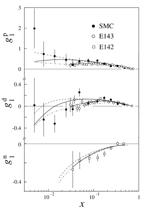
FIG. 17.: The structure functions $g_{1}^{\rm p}$, $g_{1}^{\rm d}$, and $g_{1}^{\rm n}$ at the measured $Q^{2}$ for the SMC [13], E143 [6, 7] and E142 [107] data. The solid curves correspond to our NLO fits at the $Q^{2}$ of the data points, the dashed curve at $Q^{2}_{0}$=10 GeV², and the dot-dashed curve at $Q^{2}_{0}$=1 GeV².

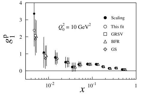
FIG. 18.: The structure function $g_{1}^{\rm p}$ evolved to $Q^{2}_{0}=10~{}$ GeV² using the scaling assumption that $g_{1}/F_{1}$ is independent of $Q^{2}$, and using NLO evolution according to our analysis and those of BFR [31], GRSV [100] and GS [101].

The measured $g_{1}(x,Q^{2})$ are then evolved from $Q^{2}$ to $Q^{2}_{0}$ by adding the correction

$$\delta g_{1}(x,Q^{2},Q^{2}_{0})=g_{1}^{\rm fit}(x,Q^{2}_{0})-g_{1}^{\rm fit}(x,Q^{2})~{},$$ (87)

where $g_{1}^{\rm fit}$ is calculated by evolving the fitted parton distributions. The resulting $g_{1}^{\rm p}(x,Q^{2}_{0})$ is shown in Table IX and Fig. 18. Also shown is the $g_{1}^{\rm p}(x,Q^{2}_{0})$ obtained by using the fits of Refs. [31, 100, 101], and by assuming scaling for $g_{1}/F_{1}$. For the lowest $x$ bin, the latter results in a considerably larger value of $g_{1}$.

C The first moment of $g_{1}^{\rm p}$

From the evolved structure function $g_{1}^{\rm p}(x,Q^{2}_{0})$, its first moment $\Gamma_{1}^{\rm p}$ is evaluated at $Q^{2}_{0}=10$ GeV², which is close to the average $Q^{2}$ of our data. The integral over the measured $x$-range is

$$\int_{0.003}^{0.7}\!\!\!\!g_{1}^{\rm p}(x,Q_{0}^{2}){\rm d}x = 0.130\pm 0.013\pm 0.008\pm 0.005~{},$$ (88)

where the first error is statistical, the second systematic and the third is the uncertainty due to the $Q^{2}$ evolution. The individual contributions to the systematic error are summarized in Table XI. The error from the evolution is mainly due to the uncertainties in the factorization and renormalization scales, in the parametrizations chosen for the parton distributions, the error in $\alpha_{s}(M_{\rm Z})$ and mass threshold effects. In addition we varied the values of $F$ and $D$ used as inputs to the fit, and of the $A_{2}$, $A_{\rm false}$, $f$, $P_{\mu}$, $P_{t}$, $F_{2}$ and of the radiative corrections used to calculate $g_{1}$. The uncertainty in the fitted parameters of the parton distributions is also included, but is found to be relatively small. These errors on $\delta g_{1}(x,Q^{2}_{0})$ are treated as correlated from bin to bin, but uncorrelated amongst each other.

The resulting $g_{1}$ using the different phenomenological analyses of the $Q^{2}$ evolution [31, 100, 101] are shown in Fig. 18. Despite their different procedures, the differences in their results are small and are covered by the error that we quote for the evolution uncertainty.

To estimate the integral for $0.7<x<1.0$ we assume that $A_{1}^{\rm p}=0.7\pm 0.3$ in this region. This is consistent with the high-$x$ data and with the expectation from perturbative QCD that $g_{1}/F_{1}\rightarrow 1$ as $x\rightarrow 1$ [104]. We obtain

$$\int_{0.7}^{1.0}g_{1}^{\rm p}(x,Q_{0}^{2}=10\,{\mathrm{GeV}^{2}}){\rm d}x = 0.0015\pm 0.0007~{}.$$ (89)

The results from our fit shown in Fig. 17 are used to evaluate $\int_{0.003}^{1.0}g_{1}^{\rm p}(x,Q_{0}^{2}){\rm d}x$ and found to be consistent with the sum of Eqs. (88) and (89).

TABLE XI.: Contributions to the error of $\Gamma_{1}^{\rm p}$

Source of the error	$\Delta\Gamma_{1}$
Beam polarization	$0.0048$
Extrapolation at low $x$	$0.0042$
Target polarization	$0.0036$
Uncertainty on $F_{2}$	$0.0030$
Dilution factor	$0.0025$
Acceptance variation $\Delta r$	$0.0014$
Momentum measurement	$0.0014$
Kinematic resolution	$0.0010$
Radiative corrections	$0.0008$
Extrapolation at high $x$	$0.0007$
Neglect of $A_{2}$	$0.0004$
Uncertainty on $R$	$0.0000$
Total systematic error	$0.0087$
Evolution error	$0.0045$
Statistical error	$0.0125$

The contribution to the first moment from the unmeasured region $0<x<0.003$ is evaluated assuming a constant $g_{1}^{\rm p}$ at $Q^{2}=10$ GeV², in agreement with a Regge-type behavior [27]. Using the average of the two lowest $x$ data points in Table IX we obtain

$$\int_{0}^{0.003}g_{1}^{\rm p}(x,Q_{0}^{2}=10\,{\mathrm{GeV}^{2}}){\rm d}x = 0.0042\pm 0.0016~{}.$$ (90)

However, to evaluate the systematic error on $\Gamma_{1}^{\rm p}$ we have assumed an error of 100% in this integral (Table XI). It should be noted that we have assumed constant Regge-type behavior at $Q^{2}=10$ GeV². If we apply the same procedure at $Q^{2}=1$ GeV² and then evolve the resulting extrapolation to $Q^{2}=10$ GeV² using the NLO fits, we obtain a value which is within $1.5\sigma$ of the assumed error. Other models describing the small-$x$ behavior of $g_{1}$ (Section II D) are also considered to check the sensitivity of our result to the small-$x$ extrapolation. A $g_{1}(x)\approx\ln x$ dependence is compatible with the error given in Eq. (90), while the $x$ behavior in the diffractive model, $g_{1}(x)\approx(x\ln^{2}x)^{-1}$, gives $\int_{0.0}^{0.003}g_{1}^{\rm p}(x,Q_{0}^{2}){\rm d}x=0.036\pm 0.016$. This model results in a larger $\Gamma_{1}^{\rm p}$, but cannot simultaneously accommodate the negative values of $g_{1}^{\rm n}$ found from our combined deuteron [13] and proton data (Fig. 16). In principle the low-$x$ contribution to the integral can be obtained from the fit to $g_{1}$, i.e. $g_{1}^{\mathrm{fit}}$. However, as known from unpolarized parton distribution functions, the behavior of the fitted distribution below the measured region is unreliable since it depends strongly on the choice of the function, renormalization, and factorization scales.

The result for the first moment of $g_{1}^{\rm p}(x,Q^{2}_{0})$ is

$$\Gamma_{1}^{\rm p}(Q^{2}_{0}=10\,{\rm GeV}^{2})\!=\!0.136\!\pm\!0.013\!\pm\!0.009\!\pm\!0.005~{}.$$ (91)

Using the results of the NLO evolutions of Refs. [31], [100] and [101] we find $\Gamma_{1}^{\rm p}(Q^{2}_{0})$ between 0.133 to 0.136 (Fig. 18). If we evaluate $g_{1}^{\rm p}(x,Q^{2}_{0})$ assuming that $g_{1}/F_{1}$ is independent of $Q^{2}$ we obtain $\Gamma_{1}^{\rm p}(Q^{2}_{0})=0.139\pm 0.014\pm 0.010$. We conclude that within the experimental accuracy of our data the different NLO QCD analyses yield consistent results for the evolution of $g_{1}$, and that $g_{1}/F_{1}$ deviates significantly from scaling at small $x$.

TABLE XII.: $\Gamma_{1}^{\rm p}$ and the contributions from different $x$ regions at $Q_{0}^{2}=$5 GeV². The results of our analysis of the SMC and the E143 data, as well as the combined analysis of the SLAC-E80/130 [1], EMC [2], SMC and SLAC-E143 [6] data are given with the statistical and systematic errors added in quadrature. Results of extrapolations are marked with an (^∗).

$x$ range	0–0.003	0.003–0.03	0.03–0.7	0.7–0.8	0.8–1	0–1
SMC	$0.004(2)^{*}$	$0.022(7)~{}$	$0.104(13)$	$0.0018(4)^{*}$	$0.0006(2)^{*}$	$0.132(17)$
E143	$0.0012(1)^{*}$	$0.010(1)^{*}$	$0.115(7)$	$0.0020(6)~{}$	$0.0006(2)^{*}$	$0.129(8)$
ALL	$0.004(2)^{*}$	$0.021(6)~{}$	$0.114(6)$	$0.0020(6)~{}$	$0.0006(2)^{*}$	$0.141(11)$

TABLE XIII.: The Ellis–Jaffe sum rule calculated with NLO QCD corrections compared to our result for $\Gamma_{1}^{\rm p}$ at $Q^{2}_{0}=$10 ${\rm GeV^{2}}$ and 5 ${\rm GeV^{2}}$ and to the combined analysis of fit the E80/E130 [1], EMC [2], SMC and E143 [6] data at $Q^{2}_{0}=$5 ${\rm GeV^{2}}$. The Bjorken sum rule calculated with NNLO QCD corrections and compared to our results on $\Gamma_{1}^{\rm p}-\Gamma_{1}^{\rm n}$ from the SMC, the combined analysis of $\Gamma_{1}^{\rm p}$ and $\Gamma_{1}^{\rm d}$ (SMC [13] and E143 [7]) and the combined analysis of $\Gamma_{1}^{\rm p}$,$\Gamma_{1}^{\rm d}$ and $\Gamma_{1}^{\rm n}$ (E142 [107]).

Experiment/Theory	$\Gamma_{1}^{\rm p}$	$\Gamma_{1}^{\rm n}$	$\Gamma_{1}^{\rm d}$	$\Gamma_{1}^{\rm p}-\Gamma_{1}^{\rm n}$
$Q^{2}_{0}=10\,\rm GeV^{2}$
SMC	$0.136\pm 0.016$	$-0.046\pm 0.021$	$0.041\pm 0.007$	$0.183\pm 0.034$
Ellis–Jaffe/Bjorken	$0.170\pm 0.004$	$-0.016\pm 0.004$	$0.071\pm 0.004$	$0.187\pm 0.002$
$Q^{2}_{0}=5\,\rm GeV^{2}$
SMC	$0.132\pm 0.017$	$-0.048\pm 0.022$	$0.039\pm 0.008$	$0.181\pm 0.035$
COMBINED(p,d)	$0.141\pm 0.011$	$-0.065\pm 0.017$	$0.039\pm 0.006$	$0.199\pm 0.025$
COMBINED(p,d,n)	$0.142\pm 0.011$	$-0.061\pm 0.016$	$0.038\pm 0.006$	$0.202\pm 0.022$
Ellis–Jaffe/Bjorken	$0.167\pm 0.005$	$-0.015\pm 0.004$	$0.070\pm 0.004$	$0.181\pm 0.003$

D Combined analysis of $\Gamma_{1}^{\rm p}$

The combined analysis of $\Gamma_{1}^{\rm p}$ includes the proton spin asymmetries for $Q^{2}>1~{}$GeV² from our data and those of Refs. [1, 2, 6] shown in Fig. 14. The EMC and SMC data were taken at an average $Q^{2}$ of 10 GeV², while for the SLAC data the average $Q^{2}$ is 3 GeV². The combined result is evaluated at an intermediate $Q^{2}$ of 5 GeV² to avoid a large $Q^{2}$ evolutions. Corrections to $g_{1}/F_{1}$ calculated at NLO are found to be up to 20–25%. The evolution of $g_{1}^{\rm p}$ to $Q^{2}_{0}=5\,\rm GeV^{2}$ (Fig. 19) is performed using the procedure of Section V B.

The data are combined on a bin-by-bin basis. The integrals $\Delta\Gamma_{1}^{i}=\int_{\Delta x_{i}}g_{1}^{\rm p}(x,Q^{2}_{0})\,{\rm d}x$ are computed for the $x$-bins of each experiment individually, starting from the published asymmetries. The $\Delta\Gamma_{1}^{i}$ which fall into the same SMC $x$-bin are first summed for each experiment and then the integral for this bin is obtained as weighted average of these sums. The weights are calculated by adding the statistical errors and systematic errors uncorrelated between the experiments in quadrature. The error and the central value of the integral in the measured region is computed using a Monte Carlo method, which takes into account the bin-to-bin correlation of the systematic errors within each experiment as well as correlations between the experiments. These correlated contributions are due to the polarizations of the beam and the target, the dilution factor, the neglect of $A_{2}$, the time dependence of the acceptance ratio, the radiative corrections, and the parametrizations of $F_{2}$ [98], of $R$ [99], and of the parton distribution functions used to evolve $g_{1}$. Correlations between the experiments arise mainly from the latter three sources. The error distributions in the Monte Carlo sampling are assumed to be Gaussian.

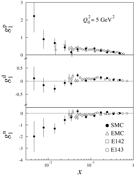
FIG. 19.: Measurements of $g_{1}^{\rm p}$, $g_{1}^{\rm d}$ and $g_{1}^{\rm n}$ evolved to $Q^{2}_{0}=$5 GeV². The SMC and E143 $g_{1}^{\rm n}$ data are obtained from $g_{1}^{\rm p}$ and $g_{1}^{\rm d}$.

The $x$ range of the combined data is $0.003<x<0.8$. The extrapolations at large and small $x$ are performed using the procedures described in Section V C. The contributions to the integral from the measured and extrapolated regions of $x$ are shown in Table XII.

The combined result for the first moment of $g_{1}^{\rm p}$ is

$$\Gamma_{1}^{\rm p}(Q^{2}_{0}=5\,\rm GeV^{2})=0.141\pm 0.011~{}~{}~{}(\mbox{\it All proton data})~{}.$$ (92)

If $A_{1}$ is assumed to be independent of $Q^{2}$, we obtain $\Gamma_{1}^{\rm p}=0.140\pm 0.012$.

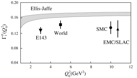
FIG. 20.: Comparison of the experimental results for $\Gamma_{1}^{\rm p}$ to the prediction of the Ellis–Jaffe sum rule.

It should be noted that the error quoted by the E143 collaboration [6] from their data alone and the error obtained from our combined analysis are comparable. The statistical uncertainties of the SMC data for $0.003<x<0.03$ introduce a larger error to $\Gamma_{1}^{\rm p}$ than the uncertainty assumed by the E143 collaboration for their extrapolation from $x=0.03$ to $x=0$. We also calculated the extrapolations from the evolved E143 and SMC data separately. The results are compared in Table XII.

The results for $\Gamma_{1}^{\rm p}$ from SMC and from the combined analysis are compared with the Ellis–Jaffe sum rule in Table XIII. The Ellis–Jaffe prediction is calculated from Eq. (56). The higher-order QCD corrections are applied assuming three active quark flavors, and using $\alpha_{s}(5~{}{\rm GeV}^{2})=0.287\pm 0.020$ and $\alpha_{s}(10~{}{\rm GeV}^{2})=0.249\pm 0.015$ corresponding to $\alpha_{s}(M_{\rm Z}^{2})=0.118\pm 0.003$ [102]. As $Q^{2}_{0}=10\,\rm GeV^{2}$ is close to the charm threshold, a small uncertainty has been included to account for the difference between the perturbative QCD corrections for three and four flavors. This uncertainty is also included in the error estimate for the Bjorken sum rule prediction presented in the next section.

We re-evaluated the first moments for all experiments at their average $Q^{2}$ using the $g_{1}$ evolution described in Section V B. In Figure 20 the results are shown as a function of $Q^{2}$. All experimental results are smaller than the Ellis–Jaffe sum rule prediction. From the combined analysis of $\Gamma_{1}^{\rm p}$ the Ellis–Jaffe sum rule is violated by more than two standard deviations. The implications of this result on the spin content of the proton will be discussed in Section VIII.

TABLE XIV.: Results for the spin-dependent structure function $g_{2}^{\rm p}$. The predicted twist-2 term for $g_{2}^{\rm WW}$ [Eq. (62)] and the upper limit obtained from $|A_{2}|<\sqrt{R}$ are also given. Only statistical errors are shown.

$x$ range	$\langle x\rangle$	$\langle Q^{2}\rangle$ (GeV2)	$\langle y\rangle$	$g_{2}$	$g_{2}^{\rm WW}$	$g_{2}^{\rm upper}$
0.006–0.015	0.010	1.36	0.72	$~{}~{}0.79\pm 75.84$	$~{}~{}0.716\pm 0.221$	$429\pm 61~{}~{}$
0.015–0.050	0.026	2.66	0.57	$~{}~{}7.14\pm 13.92$	$~{}~{}0.447\pm 0.069$	$101\pm 12~{}~{}$
0.050–0.100	0.069	5.27	0.42	$~{}~{}1.06\pm~{}4.77$	$~{}~{}0.187\pm 0.019$	$17.4\pm 4.6~{}~{}$
0.100–0.150	0.121	7.65	0.34	$-0.95\pm~{}2.92$	$~{}~{}0.037\pm 0.015$	$6.1\pm 2.8$
0.150–0.300	0.199	10.86	0.30	$~{}~{}0.20\pm~{}1.66$	$-0.073\pm 0.007$	$1.9\pm 1.2$
0.20 –0.600	0.378	17.07	0.25	$~{}~{}0.65\pm~{}0.64$	$-0.096\pm 0.005$	$0.2\pm 0.5$

VI RESULTS FOR $g_{2}^{\rm p}$ AND ITS FIRST MOMENT

A Evaluation of $g_{2}^{\rm p}(x,Q^{2})$

The spin-dependent structure function $g_{2}^{\rm p}$ is evaluated from the $A_{2}^{\rm p}$ data (Table VIII) using

$$g_{2}=\frac{F_{1}}{2Mx}\left[{\sqrt{Q^{2}}}A_{2}\left(1-\frac{\gamma(\gamma-\eta)}{1+\gamma^{2}}\right)-\frac{A_{\parallel}}{D}\left(\frac{2Mx}{1+\gamma^{2}}\right)\right],$$ (93)

from Eqs. (8) and (10) and a parametrization of $A_{\parallel}/D$ from Refs. [2, 9, 6]. We assume that $\sqrt{Q^{2}}A_{2}^{\rm p}$ and $A_{\parallel}^{\rm p}/D$ are independent of $Q^{2}$ which is consistent with the data. The new analyses of $g_{1}^{\rm p}$ or $F_{2}$ do not affect the $g_{2}^{\rm p}$ results that we published in Ref. [10] due to the limited accuracy of the data. The $g_{2}^{\rm p}$ values are given in Table XIV. The expected values of ${g_{2}}^{\rm WW}$ and the upper bound of $g_{2}$, based on the positivity limit of $A_{2}$ are also included. The statistical accuracy on $g_{2}$ is poor since the error is proportional to $1/x^{2}$ and $\sqrt{Q^{2}}$, and the data are characterized by small-$x$ and large $Q^{2}$. All values are consistent with zero.

B The first moment of $g_{2}^{\rm p}$

The Burkhardt–Cottingham sum rule predicts that the first moment of $g_{2}^{\rm p}$ vanishes (Section II G). This integral is evaluated over the measured $x$ range at the mean $Q^{2}$ of the data ($Q^{2}_{0}=5$ GeV${}^{2})$ by assuming a constant value of $\sqrt{Q^{2}}A_{2}(x)$ within each $x$ bin. We obtain

$$-1.0<\int_{0.006}^{0.6}g_{2}^{\rm p}(x,Q^{2}_{0})\,{\rm d}x<2.1~{},$$ (94)

at 90% confidence level. Our measurement of $g_{2}$ is not accurate enough to perform a meaningful extrapolation to $x=0$ using the expected $g_{2}$ Regge behavior, $g_{2}(x\rightarrow 0){\sim}x^{-1+\alpha}$ [56] and to test the sum rule. The first moment $\Gamma_{2}(Q^{2}_{0})$ can be divided into $\Gamma_{2}(Q^{2}_{0})=\Gamma_{2}(Q^{2}_{0})^{\rm WW}+\overline{\Gamma_{2}}(Q^{2}_{0})$, where $\Gamma_{2}^{\rm WW}$ is obtained from $g_{2}^{\rm WW}$ (Eq. (62)) and $\overline{\Gamma_{2}}$ from the $\overline{g_{2}}$ component. Using a parametrization of all $g_{1}^{\rm p}/F_{1}^{\rm p}$ data  [2, 9, 6] we find that the twist-2 part is, as expected, compatible with zero ($\Gamma_{2}(Q^{2}_{0})^{\rm WW}\simeq 0.001\pm 0.008.$) A violation of the sum rule caused by the $\overline{g_{2}}$ term cannot be excluded by the present data.

VII EVALUATION OF $\Gamma_{1}^{\rm p}-\Gamma_{1}^{\rm n}$ AND TEST OF THE BJORKEN SUM RULE

We first test the Bjorken sum rule at $Q^{2}_{0}=$ 10 $\rm GeV^{2}$ assuming

$$g_{1}^{\rm p}-g_{1}^{\rm n}=2\,\left(g_{1}^{\rm p}-\frac{g_{1}^{\rm d}}{1-\frac{3}{2}\omega_{D}}\right).$$ (95)

For this test we employ our present proton data and our previously published deuteron data [11, 12, 13]. For the probability of the deuteron to be in a D-state we have taken $\omega_{D}=0.05\pm 0.01$ which covers most of the published values [106]. Using the method described in Section V D to account for the correlations between errors we obtain

$$\Gamma_{1}^{\rm p}-\Gamma_{1}^{\rm n}=0.183\pm 0.034\hskip 28.45274pt(\mbox{\it$Q^{2}_{0}$~{}=~{}\rm 10\, GeV${}^{2}$\,})~{},$$ (96)

where statistical and systematic errors are combined in quadrature. The theoretical prediction at the same $Q^{2}$, including perturbative QCD corrections up to ${\cal{O}}(\alpha_{s}^{3})$ and assuming three quark flavors (Section II E 1), is $\Gamma_{1}^{\rm p}-\Gamma_{1}^{\rm n}=0.186\pm 0.002$.

We have also performed a combined analysis of all proton and deuteron data at $Q^{2}_{0}=5\,\rm GeV^{2}$ (Fig. 19). The combined $\Gamma_{1}^{\rm d}$ is obtained using the same method as described in Section V D for $\Gamma_{1}^{\rm p}$. We find

$$\Gamma_{1}^{\rm p}-\Gamma_{1}^{\rm n}=0.199\pm 0.025~{}~{}~{}~{}~{}(\mbox{$Q^{2}_{0}$=\rm 5\,GeV${}^{2}$,}$$ (97)

$$\mbox{\it All proton and deuteron data})~{}.$$ (98)

The corresponding theoretical expectation is $\Gamma_{1}^{\rm p}-\Gamma_{1}^{\rm n}=0.181\pm 0.003$, which agrees with the experimental result as shown in Fig. 21.

The structure function $g_{1}^{\rm n}$ of the neutron has also been measured by scattering polarized electrons on a polarized ³He target [5]. The re-analyzed neutron data on $g_{1}^{\rm n}$ from E142 [107] are included in the combined analysis. This requires the combination of $\Gamma_{1}^{\rm p}$, $\Gamma_{1}^{\rm n}$ and $\Gamma_{1}^{\rm d}$ via a fit constrained by the integral of Eq. (95) and the use of a Monte Carlo method to compute the $3\times 3$ correlation matrix between $\Gamma_{1}^{\rm p}$, $\Gamma_{1}^{\rm n}$ and $\Gamma_{1}^{\rm d}$. The $\Gamma_{1}^{\rm p}$ and $\Gamma_{1}^{\rm d}$ are obtained as before; $\Gamma_{1}^{\rm n}$ is obtained from the E142 data in their measured region, but the small-$x$ extrapolation is determined from the $g_{1}^{\rm n}$ values obtained from the SMC proton and deuteron data. The result is

$$\Gamma_{1}^{\rm p}-\Gamma_{1}^{\rm n}=0.202\pm 0.022~{}~{}~{}~{}~{}~{}(\mbox{$Q^{2}_{0}$=\rm 5\, GeV${}^{2}$,}$$ (99)

$$\mbox{\it All proton, deuteron and neutron data})~{}.$$ (100)

As discussed in Ref. [108], the central value and the error of $\Gamma_{1}^{\rm n}$ is very sensitive to the SMC proton and deuteron data.

The relation between $\Gamma_{1}^{\rm p}$, $\Gamma_{1}^{\rm d}$, $\Gamma_{1}^{\rm n}$ and the Bjorken sum rule is illustrated in Fig. 21 and the results are given in Table XIII. Proton, deuteron and neutron results confirm the Bjorken sum but disagree with the Ellis–Jaffe sum rule.

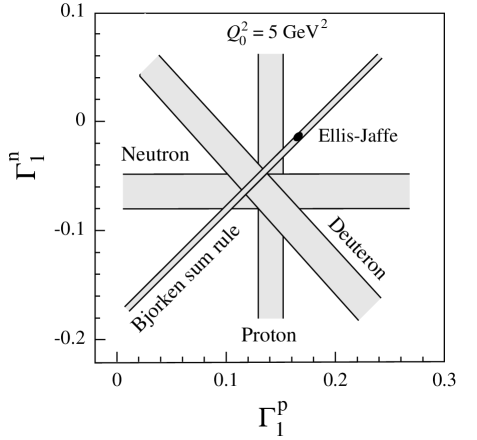
FIG. 21.: Comparison of the combined experimental results for $\Gamma_{1}^{\rm p}$, $\Gamma_{1}^{\rm n}$ and $\Gamma_{1}^{\rm d}$ with the predictions for the Bjorken and the Ellis–Jaffe sum rules. The Ellis–Jaffe prediction is shown by the black ellipse inside the Bjorken sum rule band.

VIII SPIN STRUCTURE OF THE PROTON

A The $x$ dependence of $g_{1}^{\rm n}$ and $g_{1}^{\rm p}$

In Figure 16 we show our results for $g_{1}^{\rm p}$ and $g_{1}^{\rm d}$, together with $g_{1}^{\rm n}$ obtained from $g_{1}^{\rm p}$ and $g_{1}^{\rm d}$ using Eq. (95). We find that the ratio $g_{1}^{\rm n}/g_{1}^{\rm p}$ is close to –1 at small-$x$, in contrast to the ratio $F_{2}^{\rm n}/F_{2}^{\rm p}$ which is close to +1 for $x<0.01$ [91, 109, 110]. In the QPM the difference between $g_{1}^{\rm p}$ and $g_{1}^{\rm n}$ can be written as

$$g_{1}^{\rm p}-g_{1}^{\rm n}=\frac{1}{6}[\Delta u_{\rm v}(x)-\Delta d_{\rm v}(x)+2\Delta\overline{u}(x)-2\Delta\overline{d}(x)]~{}.$$ (101)

Under the assumption of flavor symmetry in the polarized sea $(\Delta\overline{u}=\Delta\overline{d})$ [111, 112], the small-$x$ behavior of $g_{1}^{\rm n}/g_{1}^{\rm p}$ indicates a dominant contribution from the valence quarks. This is consistent with our results from semi-inclusive spin asymmetries [14] which show that $[\Delta u_{\rm v}(x)-\Delta d_{\rm v}(x)]$ is positive and that $\Delta u_{\rm v}(x)$ and $\Delta d_{\rm v}(x)$ have opposite signs. Fits of polarized parton distributions in the NLO analysis lead to the same conclusion [100, 101].

B The axial quark charges

When only three flavors contribute to the nucleon spin, the first moment of $g_{1}^{\rm p}$ can be expressed in terms of the proton matrix elements of the axial vector currents (Section II E 1)

$$\Gamma_{1}^{\rm p}(Q^{2})=\frac{C^{\rm NS}_{1}(Q^{2})}{12}\left[a_{3}+\frac{1}{3}a_{8}\right]+\frac{C^{\rm S}_{1}(Q^{2})}{9}a_{0}(Q^{2})~{}.$$ (102)

We obtain $a_{0}(Q^{2})$ from $\Gamma_{1}^{\rm p}(Q^{2})$ and the experimental non-singlet matrix elements $a_{3}$ and $a_{8}$, which are calculated from $g_{\rm A}/g_{\rm V}$ and $F/D$, as presented in Section V B. The singlet (non-singlet) coefficient function $C^{\rm S}_{1}~{}(C^{\rm NS}_{1})$ is the same as presented in Section II E 1, and $C^{\rm S}_{1}$ is computed with the coefficients $c_{i}^{\rm S}$ in the last column of Table I. If instead the coefficient from the third column were used, we would get $a_{0}^{\infty}$. Numerically, $a_{0}^{\infty}$ is smaller than $a_{0}(Q^{2})$ by 10% at $Q^{2}=10\,\rm GeV^{2}$.

From the combined analysis of all proton data we find

$$a_{0}(Q^{2}_{0})=0.37\pm 0.11~{}~{}~{}~{}~{}~{}~{}(\mbox{$Q^{2}_{0}$~{}=~{}\rm 5\, GeV${}^{2}$,}$$ (103)

$$\mbox{ \it All proton data })~{}.$$ (104)

In Table XV we compare the results with those based on SMC data only. Calculations in lattice QCD [113] agree with the measured values of both $a_{0}$ and $g_{\rm A}/g_{\rm V}$. Using $a_{3}=a_{\mathrm{u}}-a_{\mathrm{d}}$, $a_{8}=a_{\mathrm{u}}+a_{\mathrm{d}}-2a_{\mathrm{s}}$ and $a_{0}(Q^{2})=a_{\mathrm{u}}+a_{\mathrm{d}}+a_{\mathrm{s}}$, the individual contributions from quark flavors are evaluated from

$$a_{\mathrm{u}} = \frac{1}{6}\,\left[\,2a_{0}(Q^{2})+a_{8}+3a_{3}\right],$$ (105)

$$a_{\mathrm{d}} = \frac{1}{6}\,\left[2a_{0}(Q^{2})+a_{8}-3a_{3}\right],$$ (106)

$$a_{\mathrm{s}} = \frac{1}{3}\,\left[a_{0}(Q^{2})-a_{8}\right].$$ (107)

The results are given in Table XV. They indicate that $a_{\mathrm{s}}$ is negative, in agreement with the measurement of elastic $\nu$–p scattering [114, 115].

In the QPM, $a_{i}=\Delta q_{i}$. However, as discussed in Section II F, due to the $\rm U(1)$ anomaly of the singlet axial vector current the axial charges receive a gluon contribution. In the AB scheme [31] used in our QCD fit for three flavors we have

$$a_{i}=\Delta{q}_{i}-\frac{\alpha_{s}(Q^{2})}{2\pi}\Delta g(Q^{2})\;\;\;\;(i=u,d,s)~{}.$$ (108)

In this scheme $\Delta q_{i}$ is independent of $Q^{2}$. For this reason some authors consider this to be the correct scheme when assuming $\Delta s=0$ [47, 48, 49].

TABLE XV.: Results for $a_{0}$ and individual quark contributions from proton data. The results based on SMC data only are given at the average $Q^{2}$ of the data, $Q^{2}_{0}=$ 10  GeV², and at $Q^{2}_{0}=$ 5 GeV² for a direct comparison with the combined analysis of all proton data.

Data used	$a_{0}$	$a_{\mathrm{u}}$	$a_{\mathrm{d}}$	$a_{\mathrm{s}}$
SMC $\Gamma_{1}^{\rm p}(10~{}{\rm GeV}^{2})$	$0.28\pm 0.16$	$0.82\pm 0.05$	$-0.44\pm 0.05$	$-0.10\pm 0.05$
SMC $\Gamma_{1}^{\rm p}(5~{}{\rm GeV}^{2})$	$0.28\pm 0.17$	$0.82\pm 0.06$	$-0.44\pm 0.06$	$-0.10\pm 0.06$
All    $\Gamma_{1}^{\rm p}(5~{}{\rm GeV}^{2})$	$0.37\pm 0.11$	$0.85\pm 0.04$	$-0.41\pm 0.04$	$-0.07\pm 0.04$

The relation between the matrix element $a_{3}$ and the neutron $\beta$-decay constant $g_{\rm A}/g_{\rm V}$ relies only on the assumption of isospin invariance. However, in order to relate $a_{8}$ to the semileptonic hyperon decay constants $F$ and $D$, we assume $\rm SU(3)$ flavor symmetry and hence conclusions on $a_{0}$ depend on its validity. $\rm SU(3)$ symmetry breaking effects do not vanish at first order for axial vector matrix elements [116], as they do for vector matrix elements [117]. It has been suggested that in order to reproduce the experimental values of $F$ and $D$, the QPM requires large relativistic corrections which depend on the quark masses; since the s quark mass is much larger than that of u and d quarks, these corrections should break $\rm SU(3)$ symmetry. Similarly, the relations between the baryon magnetic moments predicted by $\rm SU(3)$ are badly broken [118].

The uncertainty on $a_{8}$ propagates into $a_{0}$ and $a_{\mathrm{s}}$ according to

$$\frac{\partial a_{0}}{\partial a_{8}} = -\frac{C_{1}^{\rm NS}}{4C_{1}^{\rm S}}\simeq-0.23~{},$$ (109)

$$\frac{\partial a_{\mathrm{s}}}{\partial a_{8}} = -\frac{C_{1}^{\rm NS}+4C_{1}^{\rm S}}{12C_{1}^{\rm S}}\simeq-0.44~{}.$$ (110)

The smaller magnitude of $a_{s}$ and its larger derivative with respect to $a_{8}$ make it much more sensitive to uncertainties in $a_{8}$ than $a_{0}$ [119]. For instance, the experimental test of $\rm SU(3)$ from the compatibility of different hyperon $\beta$ decays allows for a 15% modification of $a_{8}$; this would change $a_{\mathrm{s}}$ by as much as 50%, while $a_{0}$ changes by less than 10%.

A result for $a_{8}$ has been obtained from a leading-order $1/N_{c}$ expansion [120] which is much smaller than the value based on the $\rm SU(3)$ analysis. The use of this smaller value of $a_{8}$ causes $a_{0}$ to become larger, while $a_{\mathrm{s}}$ becomes positive.

In principle another source of uncertainty arises from the possible contributions of heavier quarks. The heavy quark axial current has a non-zero matrix element because it can mix with light quark operators [121]. This mixing is closely related to the $\rm U(1)$ anomaly and is directly calculable in QCD [122, 123], where the heavy quark contributions can be expressed in terms of light quark contributions. Following the analysis of Ref. [121] and using the result for $a_{0}$ of Eq. (103), the expected values for $a_{\mathrm{b}}$ and $a_{\mathrm{c}}$ for $Q^{2}\ll m_{b}^{2}$ are $-0.003\pm 0.001$ and $-0.006\pm 0.002$, respectively. In view of the current accuracy for $a_{0}$ and of the $Q^{2}$ range covered by the data, the contribution from heavier quarks can be neglected.

C The spin content of the proton

The nucleon spin can be written:

$$S_{z}=\frac{1}{2}\Delta\Sigma+L_{q}+\Delta g+L_{g}=\frac{1}{2}~{},$$ (111)

in which $\Delta\Sigma=\Delta u+\Delta d+\Delta s$ and $\Delta g$ are the contributions of the quark and gluon spins to the nucleon spin, and $L_{q}$ and $L_{g}$ are the components of the orbital angular momentum of the quarks and the gluons along the quantization axis [124]. The $Q^{2}$ dependence of the angular momentum terms analyzed in LO was studied in Ref. [125]. It is observed that the asymptotic limit ($Q^{2}\rightarrow\infty$) of the terms ($\frac{1}{2}\Delta\Sigma+L_{q}$) and ($\Delta g+L_{g}$) are about the same and equal to $\sim 1/4$.

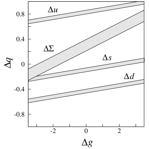
FIG. 22.: Quark spin contributions to the proton spin as a function of the gluon contribution at $Q^{2}$ = 5 GeV² in the Adler–Bardeen scheme.

In the naive QPM, $\Delta g=L_{g}=0$ and $\Delta{\Sigma}=a_{0}$. In this framework earlier experiments concluded that only a small fraction of the nucleon spin is carried by the quark spins and that the strange quark spin contribution is negative. This conclusion is in disagreement with the Ellis–Jaffe assumption of $\Delta s=a_{\mathrm{s}}=0$, which corresponds to $\Delta{\Sigma}=a_{8}\simeq 0.57$ with $L_{q}$ carrying about half of the total angular momentum. The Skyrme Model also assumes $\Delta{g}=L_{g}=0$. In a recent version of this model, where $g_{\rm A}/g_{\rm V}$ is calculated to within 4% of the experimental value, $\Delta{\Sigma}$ is found to be between 0.18 and 0.32 [126].

In QCD $a_{0}$ differs from $\Delta\Sigma$ in a scheme dependent way. In the AB scheme the determination of $\Delta\Sigma$ and the various $\Delta q_{i}$ from the measured $a_{0}$ and $a_{i}$ requires an input value for $\Delta g$. The allowed values for $\Delta{\Sigma}$ and for the $\Delta q_{i}$ are shown in Fig. 22 as a function of $\Delta g$ (Eq. (108)). We see that a value of $\Delta s=0$ and $\Delta{\Sigma}\sim 0.57$ corresponds to $\Delta g(Q^{2})\approx 2$ at $Q^{2}_{0}=5\,\rm GeV^{2}$. However, the gluon contribution $\Delta g$ could be smaller than indicated in Eq. (108) due to finite quark masses and a possibly non-negligible contribution from charm, according to the authors of Ref. [127]. In the absence of direct measurements of $\Delta g$ our results can only be compared with the estimate of $\Delta g(Q^{2})$ obtained from NLO GLAP fits to the $g_{1}$ data as in Section V B. Different estimates of $\Delta g(Q^{2})$ have been obtained. The factorization scheme used in the fit of Ref. [31] and Section V B provides $\Delta\Sigma$ and $\Delta g(Q^{2})$, while $a_{0}(Q^{2})$ and $\Delta g(Q^{2})$ are obtained in the scheme used for the fits of Refs. [100] and [101]. While the singlet distribution depends on the factorization scheme, the gluon distribution is the same in both [51]. For $Q_{0}^{2}=5\,\mathrm{GeV}^{2}$ we find $\Delta g(Q^{2}_{0})=1.7\pm 1.1$ and Refs. [128] and [100] find $\Delta g(Q^{2}_{0})=2.6$ and $0.76$, respectively. The results of Ref. [128] are based on the method of Ref. [31]. Similarly, at $Q_{0}^{2}=10\,\mathrm{GeV}^{2}$ it is found that $\Delta g(Q^{2}_{0})$ is equal to $2.0\pm 1.3$, $3.1$, and $0.89$, respectively.

D Combined analysis of $a_{0}$ from all proton, neutron and deuteron data

The analysis used to test the Bjorken sum rule can be extended to evaluate $a_{0}$, giving
( Proton, deuteron and neutron data, $Q^{2}_{0}$ = 5  GeV²) ,

$$a_{0}=~{}~{}0.29\pm 0.06~{} \hskip 14.22636pta_{\mathrm{u}}=~{}~{}0.82\pm 0.02~{},$$ , (112)

$$a_{\mathrm{d}}=-0.43\pm 0.02~{} \hskip 14.22636pta_{\mathrm{s}}=-0.10\pm 0.02~{}.$$ , (113)

An analysis of $a_{0}$ based on a different selection and treatment of experimental data has been presented in Ref. [129], with similar results.

IX CONCLUSION

A Summary

We have presented a complete analysis of our measurement of the spin-dependent structure function $g_{1}$ of the proton from deep-inelastic scattering of high-energy polarized muons on a polarized target. The data cover the kinematic range $0.003<x<0.7$ for $Q^{2}>1\>{\rm GeV}^{2}$, with an average $Q^{2}=10\>{\rm GeV}^{2}$. In addition to these data we have also shown for the first time virtual photon-proton asymmetries in the kinematic range $0.0008<x<0.003$ and $Q^{2}>0.2$ GeV². In the kinematic range $x<0.03$ our data are the only available measurements of the spin-dependent asymmetries.

The virtual photon asymmetry $A_{1}^{\rm p}\simeq g_{1}^{\rm p}/F_{1}^{\rm p}$ shows no $Q^{2}$ dependence over the $x$ range of our data within the experimental uncertainty. This observation holds when we combine our results with those from electron scattering experiments performed at smaller $Q^{2}$. However, $g_{1}$ and $F_{1}$ are predicted to evolve differently and the difference should be observable at small-$x$ in future precise measurements.

From our data on $g_{1}^{\rm p}$ together with our deuteron data we find that the ratio $g_{1}^{\rm n}/g_{1}^{\rm p}$ is close to –1 at small-$x$ ($\sim 0.005$), in contrast to $F_{2}^{\rm n}/F_{2}^{\rm p}$ which approaches +1. This suggests that either the valence quarks give a significant contribution to the net quark polarization in this region, or that the spin distribution functions of the $u$ and $d$ sea quarks are different, i.e. $\Delta\overline{u}(x)\neq\Delta\overline{d}(x)$. The data suggest a rise in $g_{1}^{\rm p}(x)$ as $x$ decreases from $0.03$ to $0.0008$. A low-$x$ extrapolation of $g_{1}$ beyond the measured region is necessary to compute its first moment $\Gamma_{1}$ and test sum rule predictions. Precise data at low $x$ are crucial for constraining this extrapolation.

The new data have initiated much theoretical activity in recent years, resulting in an extensive discussion of the NLO QCD analyses of the $x$ and $Q^{2}$ dependence of $g_{1}$ and of the interpretation of $a_{0}$ in terms of the spin content of the nucleon. As a result, we have used new methods for the evaluation of the structure function $g_{1}$ at fixed $Q^{2}$. From this evolved structure function we determined the first moment of $g_{1}$ and confirmed the violation of the Ellis–Jaffe sum rule for the proton by more than $2\sigma$. We obtain for the singlet axial charge of the proton $a_{0}(Q^{2}_{0})=0.28\pm 0.16$ at $Q^{2}_{0}=10\>{\rm GeV}^{2}$. From the fit to all currently available data, we obtain $\Delta g(Q^{2}_{0})=2.0\pm 1.3$ which in the Adler-Bardeen renormalization scheme implies the value $\Delta\Sigma\simeq 0.5$. The new data and theoretical developments now afford a first glimpse of the polarized gluon distribution and its first moment.

The Bjorken sum rule is fundamental and must hold in perturbative QCD. When corrections up to ${\cal O}(\alpha_{s}^{3})$ are included, it predicts $\Gamma_{1}^{\rm p}-\Gamma_{1}^{\rm n}=0.186\pm 0.002$ at $Q^{2}_{0}=10\>{\rm GeV}^{2}$. Using the first moments of the structure functions $g_{1}$ evaluated from our proton and deuteron data, we find $\Gamma_{1}^{\rm p}-\Gamma_{1}^{\rm n}=0.183\pm 0.034$ at $Q^{2}_{0}=10\>{\rm GeV}^{2}$ in excellent agreement with the theoretical prediction. Combining our data with all available data results in a somewhat more precise confirmation of the Bjorken sum rule.

B Outlook

New data on the spin-dependent structure functions $g_{1}$ and $g_{2}$ of the nucleon are expected in the next two years from the SMC, the E154 and E155 collaborations at SLAC, and from the HERMES collaboration at HERA. However, further knowledge is needed of the low $x$ behavior of $g_{1}$ and of the polarized gluon distribution $\Delta g(x)$ due to the limited coverage in $x$ and $Q^{2}$ of these experiments.

Future experiments are planned at various experimental facilities, including semi-inclusive polarized proton–proton scattering by RHIC SPIN [130] at BNL, semi-inclusive polarized muon–nucleon scattering by COMPASS [131] at CERN, and a similar semi-inclusive polarized electron–nucleon experiment at SLAC [132]. Furthermore, a polarized electron–proton collider experiment at HERA to study the inclusive and semi-inclusive scattering is also under consideration [133]. The non-Regge behavior of the unpolarized structure function $F_{2}$ has been observed at HERA in agreement with perturbative QCD predictions [134, 135]. The corresponding behavior predicted for the polarized spin structure function $g_{1}$ is particularly interesting due to the fact that the higher-order corrections in the polarized case are expected to be stronger [128, 136]. Also, unlike the unpolarized case where only the gluon distribution is important at low $x$, in the polarized case the singlet quark, the non-singlet quark, and the gluon distributions all play a role.

In conclusion, the study of the spin structure of the nucleon appears certain to remain active well into the next century.

X ACKNOWLEDGMENT

We wish to thank our host laboratory CERN for providing major and efficient support for our experiment and an exciting and pleasant environment in which to do it. In particular, we thank J.V. Allaby, P. Darriulat, F. Dydak, L. Foa, G. Goggi, H.J. Hilke and H. Wenninger for substantial support and constant advice. We also wish to thank L. Gatignon and the SPS Division for providing us with an excellent beam, the LHC-ECR group for efficient cryogenics support, and J.M. Demolis for all his technical support.

We also thank all those people in our home institutions who have contributed to the construction and maintenance of our equipment, especially A. Daël, J. C. Languillat and C. Curé from DAPNIA/Saclay for providing us with the high performance target superconducting magnet, Y. Lefévre and J. Homma from NIKHEF for their contributions to the construction of the dilution refrigerator, and E. Kok for his contributions to the electronics and the data taking.

It is a pleasure to thank G. Altarelli, R.D. Ball, J. Ellis, S. Forte and G. Ridolfi, for valuable discussions.

REFERENCES

- [1] SLAC E80, M.J. Alguard et al., Phys. Rev. Lett. 37, 1261 (1976); ibid. 41, 70 (1978); SLAC E130, G. Baum et al., ibid. 51, 1135 (1983).
- [2] EMC, J. Ashman et al., Phys. Lett. B206, 364 (1988); Nucl. Phys. B328, 1 (1989).
- [3] J. Ellis and R.L. Jaffe, Phys. Rev. D9, 1444 (1974); ibid. D10, 1669 (1974).
- [4] J.D. Bjorken, Phys. Rev. 148, 1467 (1966); ibid. D1 1376 (1970).
- [5] SLAC E142, D.L. Anthony et al., Phys. Rev. Lett. 71, 959 (1993).
- [6] SLAC E143, K. Abe et al., Phys. Rev. Lett. 74, 346 (1995).
- [7] SLAC E143, K. Abe et al., Phys. Rev. Lett. 75, 25 (1995).
- [8] A. Simon, “Results from the HERMES Experiment on Inclusive Polarized Deep–Inelastic Scattering”, Proceedings of SPIN96, Amsterdam; E.E.W. Bruins, “Semi-inclusive spin asymmetries in polarized deep inelastic electron scattering”, Proceedings of SPIN96, Amsterdam.
- [9] SMC, D. Adams et al., Phys. Lett. B329, 399 (1994), erratum Phys. Lett. B339, 332 (1994).
- [10] SMC, D. Adams et al., Phys. Lett. B336, 125 (1994).
- [11] SMC, B. Adeva et al., Phys. Lett. B302, 533 (1993).
- [12] SMC, D. Adams et al., Phys. Lett. B357, 248 (1995).
- [13] SMC, D. Adams et al., submitted to Phys. Lett. B, CERN-PPE/97-08, January 20, 1997.
- [14] SMC, D. Adams et al., Phys. Lett. B369, 93 (1996).
- [15] T. Pussieux and R. Windmolders, Proc. of the Symposium on the Internal Spin Structure of the Nucleon, Yale Univ., Jan. 5-6, 1994, (World Scientific, Singapore, 1995, p. 212).
- [16] R.L. Jaffe, Comments Nucl. Phys. 19, 239 (1990).
- [17] BCDMS, A. Argento et al., Phys. Lett. B120, 245 (1983); Phys. Lett. B140, 142 (1984).
- [18] B.L. Ioffe, V.A. Khoze, and L.N. Lipatov, ‘Hard Processes’, (North-Holland, Amsterdam, 1984, p. 59).
- [19] M.G. Doncel and E. de Rafael, Nuovo Cimento 4A, 363 (1971); P. Gnädig and F. Niedermayer, Nucl. Phys. B55, 612 (1973).
- [20] G. Altarelli, Phys. Rep. 81, 1 (1982).
- [21] G. Altarelli and G. Parisi, Nucl. Phys. B126, 298 (1977).
- [22] V.N. Gribov and L.N. Lipatov, Sov. J. Nucl. Phys. 15, 438 and 675 (1972).
- [23] E.B. Zijlstra and W.L. van Neerven, Nucl. Phys. B417, 61 (1994).
- [24] R. Mertig and W.L. van Neerven, Z. Phys. C70, 637 (1996).
- [25] W. Vogelsang, Phys. Rev. D54, 2023 (1996).
- [26] T. Gehrmann and W.J. Stirling, Z. Phys. C65, 461 (1995).
- [27] R.L. Heimann, Nucl. Phys. B64, 429 (1973); J. Ellis and M. Karliner, Phys. Lett. B213, 73 (1988).
- [28] S.D. Bass and P.V. Landshoff, Phys. Lett. B336, 537 (1994).
- [29] F.E. Close and R.G. Roberts, Phys. Lett. B336, 257 (1994).
- [30] M.A. Ahmed and G.G. Ross, Phys. Lett. B56, 385 (1975).
- [31] R.D. Ball, S. Forte, and G. Ridolfi, Phys. Lett. B378, 255 (1996).
- [32] J.Ellis, SPIN96 Proceedings, hep-ph/9611208.
- [33] J. Bartels, B.I. Ermoleav, and M.G. Ryskin, Z. Phys. C70, 273 (1996).
- [34] J. Bartels, B.I. Ermoleav, and M.G. Ryskin, DESY–96–025, hep–ph/9603204.
- [35] J. Kodaira et al., Phys. Rev. D20, 627 (1979); J. Kodaira et al., Nucl. Phys. B159, 99 (1979).
- [36] S.A. Larin, Phys. Lett. B334, 192 (1994).
- [37] J. Kodaira, Nucl. Phys. B165, 129 (1980).
- [38] S.A. Larin, F.V. Tkachev, and J.A.M. Vermaseren, Phys. Rev. Lett. 66, 862 (1991); S.A. Larin and J.A.M. Vermaseren, Phys. Lett. B259, 345 (1991).
- [39] A.L. Kataev and V. Starshenko, Modern. Phys. Lett. A10, 235 (1995), hep–ph/9502348; Preprint CERN/TH 94–7198 (Geneva, May 1994), hep–ph/9405294.
- [40] A.L. Kataev, Phys. Rev. D50, R5469 (1994).
- [41] SLAC E143, K. Abe et al., Phys. Rev. Lett. 76, 587 (1996).
- [42] I.I. Balitsky, V.M. Braun, and A.V. Kolesnichenko, Phys. Lett. B242, 245 (1990); erratum Phys. Lett. B318, 648 (1993).
- [43] X. Ji and P. Unrau, Phys. Lett. B333, 228 (1994).
- [44] M. Meyer–Hermann, M. Maul, L. Mankiewicz, E. Stein, and A. Schäfer, hep–ph/9605229 (8 May 1996).
- [45] J. Ellis, E. Gardi, M. Karliner, and M.A. Samuel, Phys. Lett. B366, 268 (1996).
- [46] L. Mankiewicz, E. Stein, and A. Schäfer, hep–ph/9510418 (26 Oct. 1995).
- [47] G. Altarelli and G.G. Ross, Phys. Lett. B212, 391 (1988).
- [48] A.V. Efremov and O.V. Teryaev, J.I.N.R. Preprint E2–88–287, Dubna (1988).
- [49] R.D. Carlitz, J.C. Collins, and A.H. Mueller, Phys. Lett. B214, 229 (1988).
- [50] X. Ji, J. Tang, and P. Hoodbhoy, Phys. Rev. Lett. 76, 740 (1996).
- [51] H.Y. Cheng, Preprint IP–ASTP–25–95, Academia Sinica (Taipei, Taiwan, Dec. 1995), hep–ph/9512267; Int. J. Mod. Phys. A11, 5109 (1996).
- [52] S. Adler and W. Bardeen, Phys. Rev. 182, 1517 (1969).
- [53] R.D. Ball, S. Forte, and G. Ridolfi Nucl. Phys. B444, 287 (1995).
- [54] X. Ji, Workshop in DIS Proceedings (1995) Paris.
- [55] S. Wandzura and F. Wilczek, Phys.Lett. B72, 195 (1977).
- [56] M. Anselmino, A. Efremov, and E. Leader, Phys. Rep. 261 (1995).
- [57] H. Burkhardt and W.N. Cottingham, Ann. Phys. 56, 453 (1970).
- [58] R. Mertig and W.L. van Neerven, Z. Phys. C60, 489 (1993), erratum–ibid. C65, (1995).
- [59] G. Altarelli et al., Phys. Lett. B334, 187 (1994).
- [60] N. Doble, et al., Nucl. Instr. and Meth. A343, 351 (1994).
- [61] R.L. Garwin et al., Phys. Rev. 105, 1415 (1957), M.J. Tannenbaum, Adv. in Part. Phys. I, 11 (1968).
- [62] K.L. Brown et al., TRANSPORT: CERN Yellow Report 80–04 (Geneva 1980).
- [63] C. Iselin, HALO: CERN Yellow Report 74–17 (Geneva 1974).
- [64] SMC, B. Adeva et al., Nucl. Instr. and Meth. A343, 363 (1994).
- [65] P. Schüler, Proc. of the 8th International Symposium on High Energy Spin Physics, Mineapolis, Sept. 12–17, 1988, American Institute of Physics, 1401 (1989).
- [66] C. Bouchiat and L. Michel, Phys Rev 106, 170 (1957).
- [67] F. Combley and E. Picasso, Phys. Rep. C14, 20 (1974).
- [68] R. Clifft and J.H. Field, ‘Muon Polarization Measurements in the M2 Beam at the CERN SPS’, Report EMC internal note 78/29.
- [69] A.M. Bincer, Phys. Rev. 107, 1434 (1957).
- [70] N. de Botton, et al., IEEE Transactions on Magnetics 30, 2447 (1994).
- [71] G. Scott and H. Sturner, Phys. Rev. 184, 490 (1969).
- [72] L.G. Levchuk, Nucl. Instr. and Meth. A345, 496 (1994).
- [73] D. Bardin and L. Kalinovskaya, , Version 1.00. The source code is available from http://www.ifh.de.bardin.
- [74] J. Cranshaw, Ph. D. thesis Rice Univ. (1994).
- [75] E. Burtin, Ph. D. thesis SACLAY (1996).
- [76] A. Abragam,‘The Principles of Nuclear Magnetism’, (Oxford, Clarendon Press 1961).
- [77] A. Daël et al., IEEE Trans. on Magnetics 28, 560 (1992).
- [78] J. Kyynäräinen, Nucl. Instr. and Meth. A356, 47 (1995).
- [79] D. Krämer, Nucl. Instr. and Meth. A356, 79 (1995).
- [80] SMC, B. Adeva et al., Nucl. Instr. and Meth. A372, 339 (1996).
- [81] J. Kyynäräinen, AIP Conf. Proc. 343, 555 (1995).
- [82] Y. Kisselev et al., Zh. Eksp. Teor. Fiz. 94 (2), 344 (1988); Sov. Phys. JETP 67, 413 (1988).
- [83] J.M. Le Goff et al., Nucl. Instr. and Meth. A356, 96 (1995).
- [84] SMC, B. Adeva et al., Nucl. Instr. and Meth. A349, 334 (1994).
- [85] N. Hayashi et al., Nucl. Instr. and Meth. A356, 91 (1995).
- [86] O.C. Allkofer et al., Nucl. Instr. and Meth. A179, 445 (1981).
- [87] J.M. Le Goff, A. Steinmetz, and R. Windmolders, SMC internal note, SMC/96/09.
- [88] A.A. Akhundov et al., Fortsch. Phys. 44, 373 (1996); A.A. Akhundov et al., Sov. J. Nucl. Phys. 26, 660 (1977); 44, 988 (1986); JINR-Dubna Preprints E2–10147 (1976), E2–10205 (1976), E2–86–104 (1986); D. Bardin and N. Shumeiko, Sov. J .Nucl. Phys. 29, 499 (1979).
- [89] T.V. Kukhto and N.M. Shumeiko, Nucl. Phys. B219, 412 (1983).
- [90] I.V. Akushevich and N.M. Shumeiko, J. Phys. G20, 513 (1994).
- [91] NMC, P. Amaudruz et al., Nucl. Phys. B371, 3 (1992).
- [92] NMC, P. Amaudruz et al., Z. Phys. C51, 387 (1991).
- [93] EMC, J. Ashman et al., Z. Phys. C57, 211 (1993).
- [94] SLAC E139, R.G. Arnold et al., Phys. Rev. Lett. 52, 727 (1984).
- [95] SLAC E139, J. Gomez et al., Phys. Rev. D49, 4348 (1994).
- [96] SLAC E143, K. Abe et al., Phys. Lett. B364, 61 (1995).
- [97] M. Velasco, Ph.D. thesis Northwestern Univ. (1995).
- [98] NMC, M. Arneodo et al., Phys. Lett. B364, 107 (1995).
- [99] SLAC, L. Whitlow et al., Phys. Lett. B250, 193 (1990).
- [100] M. Glück, E. Reya, M. Stratmann, W. Vogelsang, Phys Rev. D53, 4775 (1996).
- [101] T. Gehrmann and W.S. Stirling, Phys. Rev. D53, 6100 (1996).
- [102] ‘Review of Particle Properties’, Phys. Rev. D52 (1996) and off-year partial update for the 1996 edition (URL: http://pdg.lbl.gov/).
- [103] F.E. Close and R.G. Roberts, Phys. Lett. B316, 165 (1993).
- [104] S.J. Brodsky, M. Burkardt, and I. Schmidt, Nucl. Phys. B441, 197 (1995).
- [105] R.G. Roberts, ‘The Structure of the Proton’, (Cambridge University Press 1990).
- [106] W. Buck and F. Gross, Phys Rev. D20, 2361 (1979); M.Z. Zuilhof and J.A. Tjon, Phys. Rev. C22, 2369 (1980); M. Lacombe et al., Phys. Rev. C21, 861 (1980); R. Machleidt et al., Phys. Rep. 149, 1 (1987); A. Yu. Umnikov et al., University of Alberta Preprint Alberta–Thy–29–94 (1994).
- [107] SLAC E142, D.L. Anthony et al., Phys. Rev. D54, 6620 (1996).
- [108] SMC, B. Adeva et al., Phys. Lett. B320, 400 (1994).
- [109] E665, M.R. Adams et al., Phys. Rev. Lett. 75, 1466 (1995).
- [110] NMC, M. Arneodo et al., accepted in Nucl. Phys. B, hep-ex/9611022.
- [111] S. Kumano and J.T. Londergan, Phys. Rev. D44, 717 (1991).
- [112] P.J. Mulders, R.D. Tangerman, Nucl. Phys. B461, 197 (1996).
- [113] S.J. Dong and K.F. Liu, Phys. Rev. Lett. 75, 2096 (1995).
- [114] G.T. Garvey, Phys. Rev. C48, 761 (1993).
- [115] L.A. Ahrens et al., Phys. Rev. D35, 785 (1987).
- [116] J.M. Gaillard and G. Sauvage, Ann. Rev. Nucl. Part. Sci. 34, 351 (1984).
- [117] M. Ademollo and R. Gatto, Phys. Rev. Lett. 13, 264 (1964).
- [118] Z. Dziembowski and J. Franklin, Nucl. Part. Phys. 17, 213 (1991).
- [119] J. Lichtenstadt and. H. Lipkin, Phys. Lett. B353, 119 (1995).
- [120] J. Dai, R. Dashen, E. Jenkins and A.V. Manohar, Phys. Rev. D53, 273 (1996).
- [121] A.V. Manohar, Phys. Lett. B242, 94 (1990).
- [122] E. Witten, Nucl. Phys. B104, 445 (1976).
- [123] L.F. Abbott and M.B. Wise, Nucl. Phys. B176, 373 (1980).
- [124] R.L. Jaffe and A. Manohar, Nucl. Phys. B337, 509 (1990).
- [125] X. Ji, MIT Preprint MIT–CTP–2517, hep-ph/9603249 (1996).
- [126] G. Kälbermann, J.M. Eisenberg, and A. Schäfer, Phys. Lett. B339, 211 (1994).
- [127] F.M. Steffens and A. Thomas, Phys. Rev. D53, 1191 (1996).
- [128] S. Forte,‘Polarized structure functions: A theoretical update’, Invited talk at VI Blois Workshop on ‘Frontiers in Strong Interactions’, hep–ph/9511345.
- [129] J. Ellis and M. Karliner, Phys. Lett. B341, 397 (1995).
- [130] Y. Makdisi, “Polarization in hadron-induced processes at RHIC”, Proceedings of SPIN96, Amsterdam; H. En’yo, “Spin Physics at RHIC”, Proceedings of SPIN96, Amsterdam.
- [131] COMPASS Proposal, CERN/SPSLC 96-14; COMPASS Proposal Addendum 1 CERN/SPSLC 96-30.
- [132] R. Arnold in the “Round Table on Future Measurements of the Polarized Gluon Distribution in the Nucleon”, Proceedings of SPIN96, Amsterdam.
- [133] Proceedings of the ‘HERA 95–96 Workshop on Future of HERA’.
- [134] H1, S. Aid et al., Nucl. Phys. B470, 3 (1996).
- [135] ZEUS, M. Derrick et al., Z. Phys. C69, 607 (1996).
- [136] R. Kirschner and L. Lipatov, Nucl. Phys. B213, 122 (1983).