EXPERIMENTAL ASPECTS OF THE STANDARD MODEL: A SHORT COURSE FOR THEORISTS

Abstract

This is a series of lectures intended to introduce high energy theorists to the marvels of the Standard Model from an experimentalist’s point of view.

1 Introduction

The subject of the 1996 TASI summer school was “Fields, Strings, and Duality” so it is surprising, perhaps, to see a series of lectures by an experimentalist included as part of the school. I wrote these lectures because I believe with deep conviction that physics is an experimental science. It is the goal of physics to describe how the world works at its most basic and fundamental level. The students at TASI 1996 were all, for the most part, embarking on careers in theoretical physics, and I felt that I could not pass up the opportunity to teach them a little about how experimentalists view the world. The test of all scientific knowledge is experiment and the most beautiful and elegant theoretical model has no lasting value if it cannot be used to describe the results of experiments.

It is quite possible that the theories discussed at TASI 96 will not be tested experimentally for decades. On the other hand, perhaps they will be able to address anomalies in current data sets or in data that will be collected in the first half of the twenty-first century. Without an accurate crystal ball, I personally believe that it is extraordinarily important that theorists and experimentalists at least be able to talk to each other. We need to have some common language, and some understanding of each other’s techniques and the scope of the problems we are each trying to address.

As theories become more formal and mathematical and experiments become more complex and difficult, theory and experiment grow apart. It will take effort on the part of both theorists and experimentalists to stay in touch with each other. With these lectures, I hope to provide theory students with some tools to make that task easier and to motivate them to put in the effort required to forge the communication links with their experimental colleagues.

The subjects covered in these lectures are organized as follows:

• In Section 2, I will briefly discuss the Standard Model. I will list the free parameters of the Standard Model in the language of an experimentalist, and I will then describe two of the experiments that were done in the 1970’s that convinced us that the Standard Model provides an accurate description of the world.

• In Section 3, I will discuss the anatomy of an experimental result. This section is meant to introduce a student of theory to the main tools of the experimentalist; how a measurement is made, and what kinds of questions should be asked when trying to decide whether to believe a result or not. Contrary to what you may have heard, experimentalists are occasionally wrong. I’ll end this section with a discussion of the pitfalls that occasionally snare experimentalists and theorists alike.

• In Section 4, I will discuss experiments that define the Standard Model by measuring some of the free parameters of the theory. I will discuss how to measure a coupling constant, a gauge boson mass, a Yukawa coupling, and a quark mixing angle.

• The final section will concentrate on experiments that are testing the validity of the Standard Model. I will talk about searches for the Higgs and precision measurements made at the $Z$ pole. I will try to summarize the status of our current understanding of the Standard Model and what are the rogue results awaiting confirmation that could be our first hints of new physics beyond the Standard Model. I will end the lectures with a discussion of experiments of the future. Where will the data be coming from over the next few decades and what physics will they hope to address?

2 Standard Model Basics

2.1 Overview of the Standard Model

These lectures assume familiarity with the Standard Model of electroweak interactions (hereafter referred to as SM). The SM is a gauge theory where the requirement of local gauge invariance under chiral isospin transformations results in the minimal couplings to the matter fields. The gauge bosons of the theory acquire a mass via the Higgs mechanism which leads to the prediction of a massive scalar boson in the model which is yet to be discovered experimentally. The fermions in the model acquire mass via a Yukawa coupling to this Higgs field. It is worth keeping in mind that the process by which the gauge bosons acquire a mass derives from the very elegant procedure of spontaneous symmetry breaking and the existence of a finite vacuum expectation value for the Higgs field, so we at least think we understand the origins of the gauge boson masses. The fermion masses are introduced in a totally ad hoc fashion into the model.

The correct gauge group to describe nature is not predicted by the model. The simplest choice consistent with existing phenomenology was suggested in 1968 by Weinberg to be $SU(2)_{L}\times U(1)$ and reflected the known $V-A$ nature of the charged weak interactions. This choice is consistent with all experimental data to date but keep in mind that with this choice, the most striking feature of the weak interactions is simply inserted by hand. Once the gauge group is known, there are many free parameters in the model that must be determined. These are listed in Table 1.

Table 1: Free parameters in the Standard Model of electroweak interactions.

	Theorists	Experimentalists
Gauge Couplings and	$g,g^{\prime},g_{3}$	$\alpha_{EM},G_{F},\alpha_{3}$
Parameters of Higgs Field	$v,\mu$	$M_{Z},M_{H}$
Fermion	$m_{e},m_{\mu},m_{\tau},m_{\nu_{e}},m_{\nu_{\mu}},m_{\nu_{\tau}}$
Masses	$m_{u},m_{c},m_{t},m_{d},m_{s},m_{b}$
Quark	$V_{ud},V_{us},V_{ub}$
Mixing	$V_{cd},V_{cs},V_{cb}$
Angles	$V_{td},V_{ts},V_{tb}$
Lepton Mixing Angles	No conventions

For each commuting set of generators of the group, we have an independent coupling, so there are three gauge couplings $g,g^{\prime}$, and $g_{3}$ to be determined experimentally. (I’ve included $\alpha_{s}$ because the Yang-Mills Lagrangian can be extended to include an $SU(3)$ color symmetry to describe QCD). There are two parameters needed to characterize the Higgs field: the vacuum expectation value $v$, and the Higgs mass, $M_{H}=\sqrt{2}\mu^{2}$.

The experimentally accessible quantities are the coupling constants $G_{F},\alpha_{s},$ and $\alpha_{\rm EM}$, and the gauge boson masses $M_{W}$ and $M_{Z}$. The model parameters and the experimental measurables are easily related by the following set of equations:

$$M_{W}^{2} = \frac{g^{2}v^{2}}{4}$$ (1)

$$M_{Z}^{2} = \frac{g^{2}v^{2}}{2\cos^{2}\theta_{W}}$$

$$e = g\sin\theta_{W}$$

$$G_{F} = \frac{g^{2}}{8M_{W}^{2}}=\frac{1}{2v^{2}}$$

$$\tan\theta_{W} = \frac{g}{g^{\prime}}$$

$$\sin^{2}\theta_{W} = 1-\frac{M_{W}^{2}}{M_{Z}^{2}}$$

$$M_{H} = \sqrt{2}\mu^{2}$$

Very often experimental results are characterized in terms of $\sin^{2}\theta_{W}$, which determines the mixing between the neutral $SU(2)$ and $U(1)$ gauge fields that result in the physical photon and the $Z$ boson.

When the matter fields of quarks and leptons are introduced the number of free parameters proliferates appallingly. The fermion-gauge couplings are totally determined by $\alpha_{\rm EM},\alpha_{s},G_{F}$ and $M_{Z}$; however, the fermion masses coming from the Yukawa coupling of the fermions to the Higgs are all free parameters.

We have another set of parameters to introduce in the form of a rotation matrix. It appears that quark flavor eigenstates of strong interactions are not eigenstates of the weak interactions and we need to experimentally determine the $3\times 3$ mixing matrix that rotates one basis into the other. This rotation matrix is called the Cabibbo-Kobayashi-Maskawa (CKM) matrix $\!{}^{{\bf?}}$ and it is thought to contain the origins of CP violation. Finally, if neutrinos have mass (and we have no good reason to think they don’t) we have to be prepared for the neutrinos to mix as well and there is an equivalent $3\times 3$ CKM matrix for lepton sector.

In order for the SM to be completely defined, all these parameters must be measured. Once the model is defined, we can test it and in fact a major part of every high energy physics experiment now and for the past 20 years has involved testing the predictive power of the SM. The depressing but true fact is that so far, in every case, either experiment has confirmed SM predictions or experiment has been wrong!

2.2 A Little History

In 1967, Steven Weinberg published a paper $\!{}^{{\bf?}}$where he stated: “Leptons interact only with photons, and with the intermediate bosons that presumably mediate weak interactions. What could be more natural than to unite these spin-one bosons into a multiplet of gauge fields?” Most of the ingredients of what would become the SM were in place in the early 1970’s $\!{}^{{\bf?}}$, and in 1971–72 t’Hooft and Veltman showed that the theory was renormalizable. $\!{}^{{\bf?}}$

A stunning feature of the SM was that it predicted a new interaction: the weak neutral current (NC). This was the first time a fundamental interaction was predicted before it was observed. It was clearly a triumph in 1981 to see $W$’s and $Z$’s directly, but I personally believe it was the observation of the NC that convinced us the SM was right.

The easiest way to look for evidence of neutral currents is to make $Z$’s directly ($e^{+}e^{-}\to Z^{0})$ or ($q\bar{q}\to Z^{0}$). However, there was no machine capable of doing that in the early 1970’s. The mass of the $Z^{0}$ is approximately 92 GeV. None of the machines available in the 1970’s could produce 92 GeV in the center of mass!

Some of the experimental facilities operating in the early 1970’s were:

• SLAC: A linear accelerator that could produce a 22 GeV $e^{-}$ beam. They were also just turning on an $e^{+}e^{-}$ storage ring SPEAR with a maximum energy of $2.6\times 2.6$ GeV (5.2 GeV in the center of mass (CM)).

• FNAL: Just turning on with 200 GeV $p$ beam (increased to 400 GeV by end of the decade). 200 GeV $p$ on a fixed target gives approximately 20 GeV in the CM ($E_{\rm CM}=\sqrt{2E_{lab}m}$) so again they were not able to produce $Z$ bosons directly.

• CERN: A proton synchrotron produced a 28 GeV $p$ beam which could be used to make a $28\times 28$ GeV $pp$ collider (ISR). In the late 1970’s, CERN upgraded the ISR to a $270\times 270$ GeV $p\bar{p}$ storage ring which is where the $Z$ was directly produced and detected for the first time.

• BNL A 33 GeV $p$ beam on fixed target.

2.3 The Discovery of Neutral Currents

Because no machine could produce $Z$ bosons directly in the early 1970’s, the first observation of NC had to be indirect, and the most sensitive technique was neutrino scattering, where a $\nu_{\mu}$ scattered off the quarks in a nuclear target as shown in Figure  1. The hadrons in the final state could be detected (the incoming and outgoing $\nu$ were invisible to the detector), and the absence of a muon meant it was a NC event. The rate for the NC process could be compared to the rate for the corresponding charged current (CC) process where in addition to the hadrons from the breakup of the nucleon, an accompanying muon could be seen.

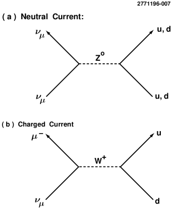
Figure 1: Diagrams for (a) neutral current and (b) charged current neutrino scattering.

It is straightforward to work out the cross sections for $\nu$ and $\bar{\nu}$ scattering off nucleons. They are discussed in detail in Quigg $\!{}^{{\bf?}}$ if you are interested. The ratios of cross sections are what can be experimentally measured most precisely and the experimentally accessible quantities are:

$$R_{\nu}\equiv\frac{\sigma(\nu N\to\nu X)}{\sigma(\nu N\to\mu^{-}X)} = \frac{1}{2}-\sin^{2}\theta_{W}+\frac{20}{27}\sin^{4}\theta_{W}$$ (2)

$$R_{\bar{\nu}}\equiv\frac{\sigma(\bar{\nu}N\to\bar{\nu}X)}{\sigma(\bar{\nu}N\to\mu^{+}X)} = \frac{1}{2}-\sin^{2}\theta_{W}+\frac{20}{9}\sin^{4}\theta_{W}$$ (3)

Measuring absolute cross sections involves a detailed knowledge of the flux of the incident $\nu$ beam and that is hard to know; however, in the ratio, both the flux and the poorly known energy spectrum of the $\nu$ beam cancel.

By just seeing $\nu N\to\nu X$ reactions, one observes NC for the first time which is a great achievement; however, one can also use the cross section ratio to extract $\sin^{2}\theta_{W}$ (or whatever your favorite third $SU(2)\times U(1)$ parameter is; the convention was to use $\sin^{2}\theta_{W}$ until LEP came on line and now $M_{Z}$ is standard). Once $\sin^{2}\theta_{W}$ is known, all the SM couplings are determined and by measuring $R_{\nu}$ and $R_{\bar{\nu}}$ one gets a wonderful consistency check. If both give the same value of $\sin^{2}\theta_{W}$, it is an indication one has chosen the right gauge structure (for example, $SU(2)_{L}\times SU(2)_{R}\times U(1)$ would predict different relations between $R_{\nu}$ and $R_{\bar{\nu}}$) and one is starting to test the predictive power of the theory.

To make neutrinos, one starts with a proton beam on a target that produces lots of secondary particles; in particular, lots of kaons and pions will be produced. The kaons and pions are selected for sign and then allowed to decay, ($\pi\to\mu\nu_{\mu},K\to\mu\nu_{\mu},K\to\pi\mu\nu_{\mu}$,) and neutrinos are produced. Muon neutrinos are strongly favored by helicity, and neutrinos or antineutrinos are selected by the charge of the meson. The experiments are hard. The major obstacle is just rate. The $\nu N$ scattering cross section is proportional to $G^{2}_{F}M_{p}E_{\nu}$ and $G_{F}$ is a small number so the cross section is small.

$$\sigma^{\nu N}_{CC} \sim 6\times 10^{-6}{\rm nb}(E_{\nu}/{\rm GeV)}/{\rm nucleon}$$ (4)

Working at the highest possible $\nu$ beam energy is clearly an advantage. FNAL with its 200 GeV $p$ beam had a great advantage for making high energy neutrinos over CERN with 30 GeV $p$, but CERN got there first.

The detector that made the discovery was the 12’ Gargamelle bubble chamber $\!{}^{{\bf?}}$. The central part of the detector was a big tank of supersaturated freon. When a charged particle passed through the supersaturated gas, it left an ionization trail. The gas was expanded suddenly after the beam pulse and bubbles formed along the ionization trail. The bubble tracks were then photographed, scanned, and measured by hand for evidence of interesting physics processes. An important feature of the detector was the ability to identify NC events by having good solid angle coverage for muons so a muon could not escape undetected. Figure  2 illustrates what CC, NC and background events would look like in the detector. The most worrisome background was a $\nu$ interacting in the material of the chamber wall, producing a neutral hadron and an escaping muon. The neutral hadron could then interact in the chamber and look like NC event.

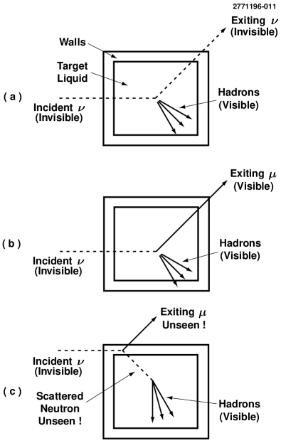
Figure 2: The signature of a NC event is illustrated in (a) where the incoming and escaping neutrinos are invisible and the signal is the observation of a hadronic cluster. A CC event is shown in (b) where the exiting muon is observed. A background event is shown in (c) where an incoming neutrino interacts in the material of the chamber wall, producing a neutral hadron which cannot be detected and a muon that escapes. The neutral hadron can then interact in the chamber and look like a NC event.

The experiment took some 300,000 pictures, 83,000 with the $\nu$ beam and 207,000 with the $\bar{\nu}$ beam. They collected twice as many events for the $\bar{\nu}$ beam since the scattering cross section was approximately one third the $\nu$ cross section due to helicity effects.

The experimenters spent a great deal of effort studying possible backgrounds to the NC sample from neutral hadrons. One particularly convincing check was that background from neutral hadrons was expected to show attenuation along the length of the chamber and they were able to show that their NC candidates had a uniform distribution along the chamber length as shown in Figure  3.

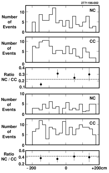
Figure 3: The number of NC and CC candidate events from the Gargamelle neutrino scattering experiment as a function of length along the chamber. The top three plots show the data for the $\nu$ beam and the bottom three plots show the $\bar{\nu}$ beam data.

From the ratio of the number of NC to CC events, they were able to conclude “$\sin^{2}\theta_{W}$ is in the range 0.3–0.4.” They conservatively claimed “if the events are due to NC, then $R_{\nu}$ and $R_{\bar{\nu}}$ are compatible with the same value of $\sin^{2}\theta_{W}$.”

This experiment has been repeated many times since 1973. The best experiment to date was done using a 450 GeV proton beam and the CDHS detector and was published in 1990 $\!{}^{{\bf?}}$. It gives, using similar techniques:

$$\sin^{2}\theta_{W}=0.228\pm 0.013(m_{c}-1.5)\pm 0.005({\rm experimental})\pm 0.003({\rm theoretical})$$ (5)

where $m_{c}$ is the charm quark mass.

2.4 The Discovery of Neutrinoless Neutral Currents

Neutral currents were discovered by neutrino scattering experiments. The coupling that was observed was consistent with the SM predictions; however, there are many other terms in the SM Lagrangian involving NC apart from neutrino-quark interactions. In particular, there are NC terms in the Lagrangian that do not involve neutrinos (e.g., electron-quark scattering through $Z$ exchange). These terms are particularly interesting because electron-quark scattering can take place via $Z$ or $\gamma$ exchange as shown in Figure 4 and the two processes can interfere. As I’ll show, this interference allows one to explore the parity violating nature of the NC interaction.

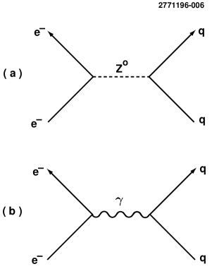
Figure 4: The two processes, (a) $Z$ exchange and (b) $\gamma$ exchange, which can contribute to electron-quark neutral current scattering.

There were two approaches that experimentalists used to probe the electron-quark coupling. The first approach was to scatter high-energy polarized electrons off of a nuclear target. This was first done at SLAC and I’ll talk about it in some detail. The other was to use atoms. The $e^{-}$ in an atom interacts with the nucleus both via the usual EM interaction and by $Z$ exchange. The immediate consequence is that the atomic Hamiltonian does not conserve parity. Everything you learned about stationary states of atomic systems being eigenstates of the parity operator was incorrect (although a good approximation)!

In the late 1970’s, experiments in atomic bismuth failed to detect parity violation, in contradiction with the SM expectation  $\!{}^{{\bf?}}$. The early atomic physics results were wrong. Later experiments in the early 1980’s agreed with the SM predictions $\!{}^{{\bf?}}$ but by that time the SLAC experiment had already confirmed the SM predictions for electron-quark couplings in 1978–79.

The basic idea of the electron-quark scattering experiments is that the scattering cross section is the square of the sum of the weak and EM amplitudes, $A_{WK}$ and $A_{EM}$, which can interfere:

$$\sigma\sim|A_{EM}+A_{WK}|^{2}=A_{EM}^{2}\left(1+\frac{2A_{EM}A_{WK}}{A_{EM}^{2}}+\frac{A_{WK}^{2}}{A_{EM}^{2}}\right)$$ (6)

At low $Q^{2}$ ($Q^{2}<10$ GeV²), $A_{EM}\gg A_{WK}$ and the last term can be dropped. The interference term, however, can be detected.

If we treat the NC as current-current interaction with vector ($V$) and axial vector ($A$) parts (recall the CC is $V-A$ but the NC is much more complicated) then

$$A_{WK}=J_{e}J_{q}=(V_{e}V_{q}+A_{e}A_{q})+(V_{e}A_{q}+A_{e}V_{q})$$ (7)

where the subscripts $e$ and $q$ refer to the electron and quark currents. The first term is a scalar ( $(V_{e}V_{q}+A_{e}A_{q})=A_{WK,{\rm scalar}}$) and is extraordinarily difficult to detect. The second term, ($(V_{e}A_{q}+A_{e}V_{q})=A_{WK,{\rm pseudoscalar}}$) however, is a pseudoscalar and has a very nice signature because it changes sign under parity transformation. It is straightforward to show that if we define the asymmetry, $\delta$, as the difference in the scattering cross section for left and right handed scattering divided by the sum, then:

$$\delta = {\sigma_{R}-\sigma_{L}\over\sigma_{R}+\sigma_{L}}$$ (8)

$$= {2(A_{WK,{\rm pseudoscalar}}A_{\rm EM})\over A_{EM}^{2}}$$ (9)

where $\sigma_{R},\sigma_{L}$ are the cross sections for right and left handed coordinate systems and the handedness of the coordinate system is determined by, for example, the longitudinal polarization of the incoming $e^{-}$ beam.

The asymmetry is small! At $Q^{2}\sim 10$ GeV², the ratio of the weak and electromagnetic amplitudes can be estimated:

$$A_{EM} \sim {4\pi\alpha_{EM}\over q^{2}}$$ (10)

$$A_{\rm WK} \sim G_{F}$$ (11)

$$\delta \sim {G_{F}q^{2}\over 4\pi\alpha_{EM}}$$ (12)

$$\sim 10^{-4}$$ (13)

In the SLAC experiment that discovered neutrinoless NC, high-energy polarized electrons were scattered off of an unpolarized deuterium target $\!{}^{{\bf?}}$. The scattered electrons were detected at a fixed scattering angle in the lab which corresponds to a fixed energy of the scattered electron. It is straightforward (but tedious) to start from the SM Lagrangian and calculate the expression for the asymmetry in scattering left versus right handed electrons $\!{}^{{\bf?}}$.

To measure an asymmetry of $10^{-4}$ to 10% precision, one needs $10^{10}$ events. Clearly one cannot count scattered electrons one by one. The experiment used a slightly different philosophy from the usual single particle counting techniques common in high energy physics. Instead of counting the scattered electrons individually, the detector integrated the signal and measured a current of scattered electrons on each beam pulse.

Figure  5 shows an overview of the experiment. At the gun end of the linac, they started with a polarized $e^{-}$ source. The polarized $e^{-}$ source was really very cute. Usually in a linear accelerator, one uses a thermionic cathode which is heated up and electrons are boiled off, collected, and used to produce an unpolarized beam. To make polarized electrons, they replaced the thermionic cathode with a gallium arsenide crystal. The electrons were polarized by optically pumping electrons from the $j=3/2$ valance band to $j=1/2$ conduction band of the crystal with a circularly polarized laser beam (710 nm light). Starting from the valance band a circularly polarized photon has $\Delta j_{Z}=+1~{}{\rm or}-1$. The Clebsch-Gordon coefficients are favorable and one gets $3$ times as many electrons in one $m_{j}$ level as the other in the upper state conduction band, which polarizes the upper state. This is illustrated schematically in Figure  6.

Figure 5: Overview of the SLAC polarized electron scattering experiment that discovered neutrinoless NC.

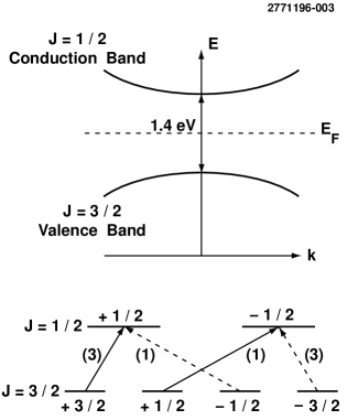
Figure 6: The energy levels of the conduction band and valence band of GaAs. A circularly polarized laser which induces transitions can polarize the upper state as shown.

To get the electrons out of the crystal conduction band, they coated the surface with cesium and oxygen which produced a negative work function. The electrons could escape and their polarization was preserved. The circular polarization of the laser controlled the polarization of the $e^{-}$ beam and it could be changed on a pulse by pulse basis in a random way. This technique theoretically could produce an electron beam with 50% polarization. In practice, the average electron beam polarization was 37%.

The beam was then accelerated down the linac with very little loss of polarization. At the end of the linac, the beam was deflected into the beam switchyard onto the deuterium target.

The scattered $e^{-}$ flux was measured with 2 independent detectors, both measuring the total charge passing through them. The polarization of the spent beam was determined with a Möller polarimeter, taking advantage of the asymmetry in the cross section for a longitudinally polarized electron scattering on polarized target electrons. The parity violating asymmetry that was the signature for NC was computed by counting electrons scattered into the detector when the electron beam was left handed versus right handed.

The challenge of this type of experiment is not just to measure an asymmetry of one part in $10^{4}$, but to convince yourself you are measuring the correct asymmetry! A great deal of attention was paid to ensure that all possible instrumental asymmetries were at the $10^{-5}$ level or smaller. The final result was

$$\sin^{2}\theta_{W} = 0.222\pm 0.018.$$ (14)

It was a demonstration of the power of the SM that with a single value of the parameter $\sin^{2}\theta_{W}$, it could account in detail for the strengths of very disparate processes: both the SLAC polarized electron scattering experiment and the neutrino scattering experiments. And that is why, with the SLAC result, the high energy community was convinced, even before the $Z$ was found, that the SM was correct and that $SU(2)_{L}\times U(1)$ was the correct gauge group to describe the world around us.

3 Anatomy of an Experiment

3.1 Overview

Having talked about the experiments done in the 1970’s that discovered NC, I now want to fast forward to present day. I will start by describing the landscape of experimental high energy physics today. What are the current machines and detectors? Where is the physics happening?

There are 3 basic types of machines currently operating: $e^{+}e^{-}$ colliders, a $p\bar{p}$ collider, and fixed target experiments. The $e^{+}e^{-}$ colliders are machines where bunches of $e^{+}$ and $e^{-}$ with equal energy and opposite momenta collide. All of the beam energy is available in the center of mass(CM) as illustrated in Figure 7(a), and the CM is the lab frame. The dominant process is annihilation. Rates at these machines tend to be low because the annihilation cross section is small and falls with increasing energy.

At the Fermilab (FNAL) $p\bar{p}$ collider, often called the Tevatron, bunches of $p$ and $\bar{p}$ collide with equal and opposite momenta as shown in Figure 7(b). The partons in the protons that interact carry only about 1/6 of the energy of the incident proton, although the distribution of the fraction of energy carried by the partons has a long tail. The CM energy of the parton-parton interaction is not known event by event, and, in fact, the CM frame of the interaction and the lab frame may not be the same. The CM may have appreciable boost along the beam direction in the lab. The total inelastic cross section is very large, which results in large backgrounds to the signals one wants to see. There are lots of events and sorting between interesting and uninteresting events is a challenge.

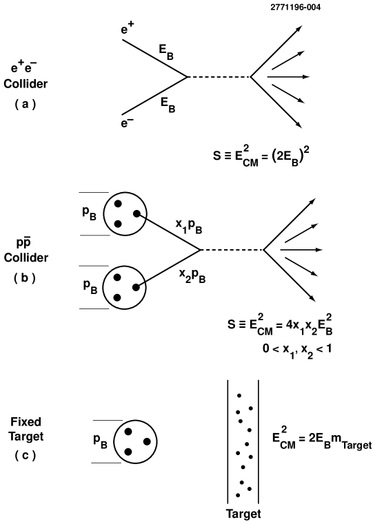
Figure 7: The basic types of collisions are illustrated.

Fixed target experiments usually involve production of a secondary beam of particles to be studied by slamming protons into a target. Examples are production of kaon beams to study rare $K$ decays or CP violation in the $K$ system, or production of $\nu$ beams to study $\nu$ oscillations or for deep inelastic scattering experiments. Here, the CM energy available is only a fraction of the beam energy as illustrated in Figure 7(c).

Table  2 shows the kind of physics accessible with the major high energy physics facilities in the world by type of collision and CM energy. I have not tried to be exhaustive and only listed the main players at each machine, excluding a host of smaller experiments, especially in the fixed target program. I will mostly talk about the CDF, ALEPH, and CLEO experiments.

Table 2: The major experiments currently operating.

Machine	Lab	Detector	Type of	$\sqrt{s}$	Physics
			Collision	(GeV)
Tevatron	FNAL	CDF	$p\bar{p}$	1800	$t,W,Z$
		D0
HERA	DESY	H1	$ep$	$300\times 820$	QCD, exotics
		ZEUS
LEPI(II)	CERN	ALEPH	$e^{+}e^{-}$	92(195)	$Z(W$,Higgs)
		L3
		OPAL
		DELPHI
SLC	SLAC	SLD	$e^{+}e^{-}$	92	$Z$
CESR	CORNELL	CLEO	$e^{+}e^{-}$	10.58	$B$
BEPC	CHINA	BES	$e^{+}e^{-}$	4	$\tau,\psi$
AGS	BNL	30 GeV $p$ $\to K$ beams
LAMPF	LANL	$\bar{\nu}_{\mu}$ beams
Tevatron	FNAL	1TeV $p$ $\to\nu,K$ beams
SPS	CERN	450GeV $p$ $\to\nu,K$ beams

3.2 Detectors

When the beams collide at an accelerator, physics happens: particles that we want to study emerge. The interaction region is instrumented with a detector that is designed to record as much information as possible about what is emerging from the beam collision.

The form of the detector depends in its gross geometry on the accelerator type. At storage rings where the lab frame is also the CM frame for the interaction, outgoing particles from the interaction are nearly isotropically distributed about the collision point and detectors reflect that fact. The detectors try to surround as much of the solid angle around the interaction point as possible, given practical and financial constraints. Typically such detectors are forward$-$backward and azimuthally symmetric to reflect the production symmetry and cover over $90\%\times 4\pi$ of the solid angle. A typical collider detector is shown in Figure 8

Picture converted to gif file

Figure 8: A schematic view of the ALEPH detector which operates at the LEP collider. (http://alephwww.cern.ch/alephgif/alephpict.html)

In a fixed target experiment, the interactions are very boosted. The experiments can cover most of the solid angle in the CM frame by being very long and narrow in the lab frame as shown in Figure 9.

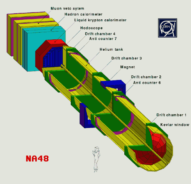
Figure 9: A schematic view of the NA48 detector which is a fixed target experiment operating the the kaon beam at CERN. (http://www1.cern.ch/NA48/Welcome/images/detector.html)

It is not possible to describe a generic detector. Each detector is individually designed to match the machine at which it runs; however, all detectors are composed from a fairly consistent set of building blocks which can be easily described, although the execution or techniques used on different experiments will vary widely.

The basic components of all detectors are:

• charged particle tracking which determines the momentum and charge of charged tracks

• electromagnetic (EM) calorimetry which identifies photons and electrons and measures their energy and direction.

• hadron calorimetry which is used to measure the energy of jets of hadrons

• muon detection which is used to identify muons

• particle identification of various sorts to distinguish different types of hadrons, particularly pions and kaons.

I will briefly discuss the various detector elements and how they are most commonly used. $\!{}^{{\bf?}}$

Charged Particle Tracker

A charged particle tracker, usually a drift chamber, is at the heart of most experiments. A basic drift chamber is made of cathode wires at negative high voltage (-HV), and anode wires at positive high voltage (+HV), enclosed in a gas volume. Incoming charged particles passing through the gas ionize the atoms in the gas. In the ionizing encounter, electrons are liberated and drift in the applied electric field towards the anode as shown in Figure 10. To measure the position of a track, a clock is started when the particle is produced (at the beam crossing) and stopped when the pulse height on a wire exceeds a preset value. Associated with each wire there will then be a time $t_{i}$. Using $d_{i}=v_{D}t_{i}$ where $v_{D}$ is the drift velocity of electrons in the gas, one can infer the distance from the wire to where the track ionization segment came from. By joining hits, one defines the track of the incident charged particle.

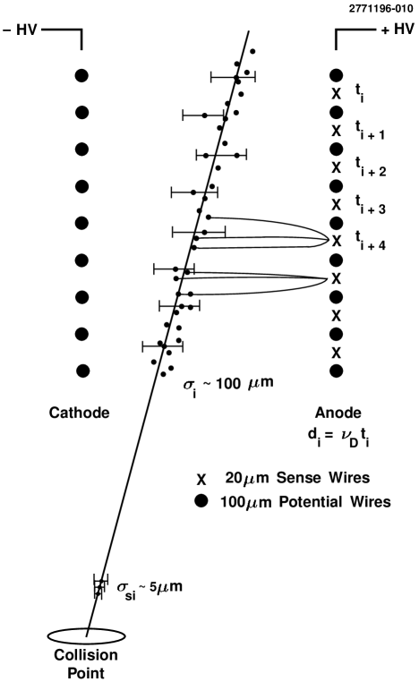
Figure 10: A schematic view of how a drift chamber operates. An incoming charged particle ionizes the gas. The liberated electrons drift in the applied electric field to the anode wire where a signal is recorded.

Precision silicon tracking devices work on the same physics principle, although the anode and cathode in a silicon detector are no longer wires but electrodes etched on a thin silicon wafer. Silicon detectors are usually placed right around the beam pipe and provide high resolution position measurements on tracks close to the interaction point.

The entire tracking volume is usually enclosed in a uniform magnetic field and from the curvature of tracks one measures the particle’s momentum.

Drift chambers are the most versatile of all detector elements. In addition to measuring momentum and charge, tracks left by charged particles can be extrapolated back to the interaction point. Tracks with significant impact parameters to the beam crossing point, or that can be combined to form a displaced vertex as illustrated in Figure 11, may come from the decays of long-lived particles. For example, the silicon vertex resolution for the LEP experiments is $\sim 200\mu$m while the typical decay lengths of heavy flavor $(\tau,D,B)$ particles are $\sim 2$ mm.

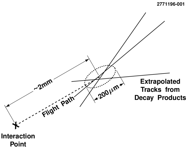
Figure 11: A sketch of a typical $B$ meson decay as seen by the LEP collider experiments. The mean flight path of a $B$ meson at LEP is approximately 2mm, and the vertex resolution of the silicon detectors is about 200 $\mu$m.

Figure 12 shows tracks in a typical collider detector. The dots are hits on anode wires. The pattern recognition software is responsible for joining the dots into tracks.

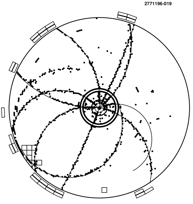
Figure 12: A typical event in the CLEO tracking chambers. The dots are hits on anode wires and the lines are drawn by the pattern recognition software which is responsible for joining the dots into tracks.

Electromagnetic Calorimeter

Most experiments have some form of electromagnetic (EM) calorimeter. EM calorimeters are devices where electrons and photons will shower in an alternating sequence of bremsstrahlung and pair production, giving up all their energy. This is the primary form of photon detection. Photons deposit all their energy in the EM calorimeter, and they are identified as photons (as opposed to electrons which will also shower) because there is no charged track pointing at the cluster of energy. The photons can then be combined with other photons to reconstruct $\pi^{0}$’s from their decay $\pi^{0}\to\gamma\gamma$.

EM calorimeters are also very powerful as $e^{-}$ detectors. An electron is identified by matching the energy of a shower in the calorimeter to the momentum measured on a charged track pointing to the cluster. Electrons are easily separated from hadrons and muons, which deposit much less energy as shown in Figure 13.

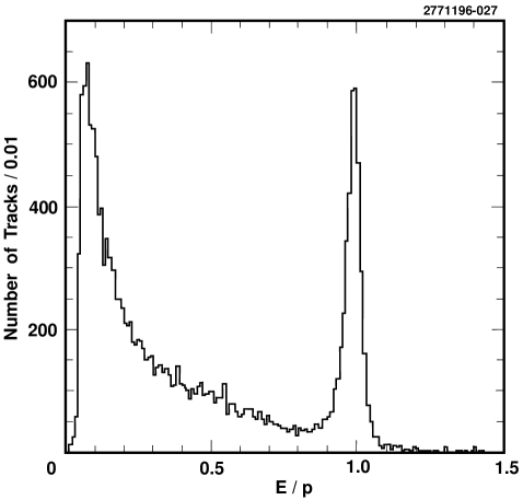
Figure 13: A plot of the ratio of energy (E) in a cluster in the CLEO EM calorimeter to the momentum (p) of a track pointing to that cluster. The peak at 1 is due to electrons. The clusters with E/p less than 1 are mostly hadrons.

EM calorimeters are built using a variety of techniques. The most precise are the crystal calorimeters which are constructed of blocks of CsI, NaI, or BGO. The entire EM shower is contained in the uniform crystal blocks with dimensions typically 5 cm $\times$ 5 cm $\times$ 30 cm deep. Adjacent blocks are summed to reconstruct the shower.

An alternate technique is a sampling shower detector typically made of a lead-scintillator sandwich. Thin lead plates are alternated with a scintillator such as liquid argon. The shower forms in the lead and is then sampled in the scintillator. EM calorimeters can be small. The CLEO CsI calorimeter with a depth of 30 cm can fully contain a 5 GeV photon with little light leakage. The ALEPH Pb-liquid argon EM calorimeter identifies electrons with tens of GeV of energy and is only 40 cm in radial depth.

Hadron Calorimeters

Hadron calorimeters, in contrast to EM calorimeters, are big. When a strongly interacting particle goes through material, there are elastic and inelastic interactions with nuclei in the material, producing secondary hadrons. Hadron calorimeters typically use a sampling technique with plates of a dense high $Z$ material such as uranium or iron sandwiching a scintillating material or ionization detector where the shower is sampled. Again, the idea is to get a particle to give up all its energy in the calorimeter. Typical hadronic interaction lengths of materials such as iron are 15-20cm, and many interaction lengths are needed for an efficient detector. Since the hadron calorimeter in a colliding beam detector has to go outside the drift chamber and EM calorimeter, this can be a lot of iron! The ALEPH hadron calorimeter is 1.2m thick, starting at a radius of 3m from the beam line.

The most important use of a hadron calorimeter is to measure the energy of dense jets of particles. In CDF, the energy of the jet is used to infer the energy of the underlying parton that produced the jet, and we will come back to this when I talk about the measurement of the top quark mass.

An important use of both EM and hadron calorimeters is to detect neutrinos in an event. Neutrinos will leave no measurable signal in the detector, so the only hope is to detect them indirectly. This is particularly important for the $W$ and top quark discoveries and mass measurements at a hadron machine. The experiments use a missing momentum technique. I mentioned that at a hadron machine, the CM of the parton-parton collision is not necessarily the lab frame. Since fragments of the parent proton and antiproton escape down the beam pipe in the very forward direction, there is no way to use conservation of total momentum in the event to infer the momentum of the unobserved neutrino. However, the components of the momentum in the plane transverse to the beam line ($p_{T}$) can be measured for all the observed decay products by using the vector sum over the energy deposited in the calorimeters, and that should be zero before and after the collision. Therefore, the neutrino transverse momentum can be inferred as the negative of the vector sum of all the transverse momenta detected in the event.

Muon Detectors

Muons are very penetrating and so muon detectors are typically planar drift chambers outside of the calorimeters and the magnet flux return. Any charged particle that makes it through that many interaction lengths of material is identified as a muon.

Particle Identification

I have already talked about how to identify electrons, muons and photons. Many experiments find it useful to also distinguish protons, pions and kaons. There are currently experiments with very sophisticated particle identification systems based on differences in the pattern of Cerenkov radiation emitted by the various particle species. Low energy experiments can get some information from time of flight or ionization losses in their drift chambers, but the information is limited.

Examples

Figure 8 shows the ALEPH detector which operates at the LEP $e^{+}e^{-}$ storage ring with $E_{CM}=92$GeV. The CLEO detector, which operates at 10.58 GeV in the CM, is shown in Figure 14 and CDF, which runs at the 1.8 TeV $p\bar{p}$ collider at FNAL, is shown in Figure 15. As you can see, the three detectors are very similar in many ways, but each is individually optimized to the physics opportunities at its particular machine.

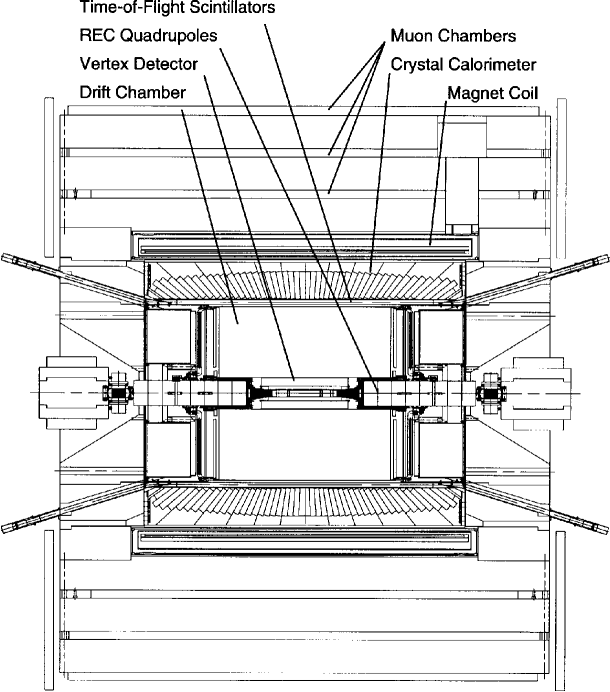
Figure 14: A schematic of the CLEO detector.

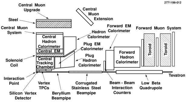
Figure 15: A schematic quarter view of the CDF detector showing the major detector elements. (http://www-cdf.fnal.gov/experiment/drawings/bw quadrant runi.ps)

3.3 Detector Operation

When the beams at the accelerator collide (or a kaon decays or a $\nu$ interacts in a fixed target experiment), physics, as I said, happens. The first thing that the experiment has to decide is whether or not an interaction of interest has occurred at a particular beam crossing or beam spill. This decision is crucial. If something interesting happens, then the event will be read out, which takes time (meaning subsequent events will be missed). In the trade, the process by which the experiment decides whether or not an event is interesting is called the trigger. Too loose or indiscriminate of a trigger will result in lots of dead time for the experiment so good data will be lost. Too tight or selective of a trigger means interesting physics may be thrown away.

For $e^{+}e^{-}$ machines, triggering for most types of events is quite straight forward. Cross sections are low. Fairly simple requirements requiring evidence of a minimum number of charged tracks in the detector or a minimum threshold for energy deposited in the calorimeter will yield a trigger that is essentially without deadtime but still preserves 99% efficiency for $e^{+}e^{-}$ annihilation events.

For $p\bar{p}$ machines and fixed target experiments, the trigger is difficult and must be carefully thought through. Interactions occur at FNAL almost every beam crossing. Great care must be taken to suppress unwanted background but still preserve the $W,Z,$ and $t$ events one wants to study. Kinematics helps because heavy objects will not have significant boost in the lab frame. When a heavy object ($Z,W,t$) is produced, its decay products can have a lot of energy transverse to the beam direction, while the uninteresting events send most of the beam energy down the beam pipe.

To give a quantitative comparison, the total annihilation cross section at LEP is $\sigma(e^{+}e^{-})\sim 32$nb. At FNAL, $\sigma(p\bar{p})\sim 50$ mb (6 orders of magnitude greater).

Once the detector is triggered, we read out events. In Figures 16, 17, and  18, I show a $B$ meson decay from CLEO, a $Z$ decay from ALEPH and a $Z$ decay from CDF. The underlying physics process in these events could not have been identified by looking at the event pictures alone. It is only by a careful selection process that these events can be identified. However, it is an amusing exercise to speculate what is going on in individual events. Looking at event pictures is fun, instructive, and keeps us attached to the real world, but it is not how we do physics!

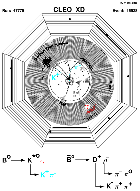
Figure 16: An event picture from CLEO showing two reconstructed $B$ meson decays.

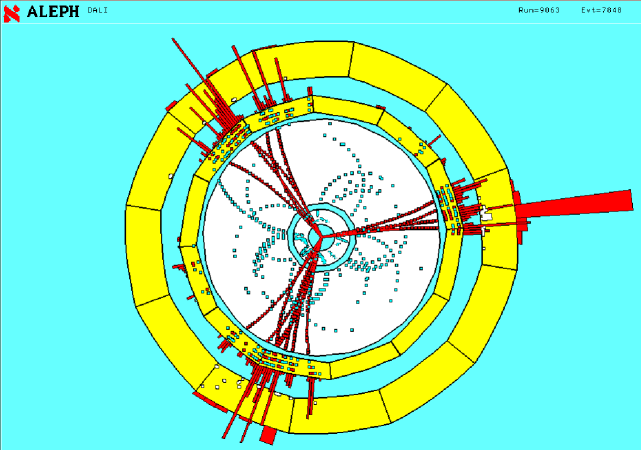
Figure 17: An event picture from Aleph showing a $Z$ decay to two quarks making two jets and with hard gluon radiation making a third jet. (http://alephwww.cern.ch/WWW/daligif/dc009063 067848 cal yel 2 w.gif)

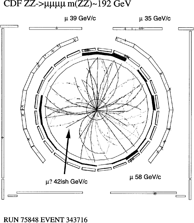
Figure 18: An event picture from CDF showing a $ZZ\to\mu\mu\mu\mu$ decay. Three of the muons are identified and momenta of the tracks are given. (http://www-cdf.fnal.gov/physics/ewk/mmmm.ps)

3.4 Data Analysis

A typical experiment may have millions of events recorded. A typical physics analysis may end up with a few hundred events. An analysis searching for a rare process may end up with a sample of only 10 or 20 events. One has to develop a procedure to select events characteristic of the physics process one wants to study but without unnecessary bias. This is an extraordinary challenge, especially when one considers the magnitude of the winnowing that must occur.

The primary tool that experimenters have to help them develop a selection procedure is called “the Monte Carlo” (MC). The Monte Carlo has two parts: the physics simulation and the detector simulation.

Monte Carlo

Starting from a differential cross section that describes our best understanding of the physics happening at a given CM energy, an event generator will generate momentum 4 vectors for a properly distributed sample of events. For example, if we were interested in studying $Z$ decays at 92 GeV, the physics MC would generate $Z$ bosons and then decay them to the correct proportions of leptons and quarks according to whatever model (such as the Standard Model) we specified.

The Standard Model tells us how to distribute the 4 vectors of quarks and leptons. We then need some model of hadronization to give us the physical mesons produced, and then the mesons are decayed according to whatever we know about their branching ratios and lifetimes. This procedure keeps going until one has a set of 4 vectors for long-lived particles that will actually end up in the detector, and is schematically illustrated in Figure 19.

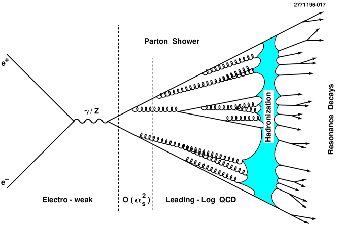
Figure 19: The fragmentation process is illustrated where partons evolve into the particles we detect in our detector. (http://alephwww.cern.ch/ALEPHGENERAL/reports/figures/qcd/partsh.gif)

A word of warning: the physics MC is only as good as the physics we put into it! If we have neglected some physics in the MC that is present in the data, we will get discrepancies between what the MC thinks we should be seeing in our data, and the data we collect. It is always important to understand what the limitations in the physics inputs to simulations are.

The second part of the MC is used to simulate how events will appear in the detector and it is called the detector simulation. Here one takes the 4 vectors of the stable (long lived) particles produced by the physics simulation and propagates them through the detector. The detector simulation, for example, simulates the multiple Coulomb scattering and energy losses as the particle passes through the beam pipe. It propagates the particle through the drift chamber and generates MC data as simulated signals on drift chamber sense wires. It simulates the EM shower in the calorimeter and so on. The detector simulation is hugely expensive in terms of computer time.

The great value of the MC is that one can generate a sample of “fake data” or “MC data” to test an analysis procedure on. One can determine the effect that analysis selection criteria will have on efficiency, one can study potential backgrounds, and far and away the most important function of MC is that one can, in an unbiased way, come up with criteria to select a signal.

It is appallingly easy when one is looking for rare processes with small numbers of signal events and with large backgrounds to end up enhancing a statistical fluctuation. I will show you some published examples in a few pages. The only way to avoid that is to use MC data to determine event selection and background suppression techniques before ever looking at the data.

Sample Analysis

I am going to illustrate for you how an analysis proceeds. I am going to choose an example of an analysis to measure the rate for a $B$ meson to decay to the final state $D^{*}\ell\nu$. I choose this particular example because I will use this decay rate in the next section as an example of how to measure CKM mixing angles. For experimental reasons, we use the decay chain: $D^{*+}\to D^{0}\pi^{+},D^{0}\to K^{-}\pi^{+}$. The experimental quantity that is measured is the branching ratio which can be related to the decay rate by the measured $B$ lifetime:

$${\rm Br}(B\to D^{*}\ell\nu)=\frac{\Gamma(B\to D^{*}\ell\nu)}{\Gamma(B\to{\rm all})}=\tau_{B}\Gamma(B\to D^{*}\ell\nu)$$ (15)

• Event Selection: During this stage of the analysis, we come up with criteria for selecting specific events to study. In the case of $B\to D^{*}\ell\nu$, we look for events with a $D^{*}$ and a lepton in them, with kinematics consistent with coming from $B\to D^{*}\ell\nu$ decay. We use the MC to study both signal events (for which we want a high efficiency) and background events (which we want to suppress) and optimize our selection criteria accordingly.

• Determination of Backgrounds: For this analysis, we may have $D^{*}\ell$ pairs that are not from $B\to D^{*}\ell\nu$ decays. We can use the MC to help evaluate the backgrounds, but unless the MC is a perfect description of $B$ decay, we cannot trust it to absolutely predict the background rates. Therefore we try to evaluate as many backgrounds as possible using the data.

• Efficiency: To evaluate the efficiency of our selection criteria, we generate $B\to D^{*}\ell\nu$ events using MC and pass them through our detector simulation. We then analyze these MC events the same way as we analyze data. It is reasonable to ask: why trust the event generator? We don’t. We need to vary the physics generator over the acceptable parameter space and see how the efficiency of the analysis is affected. Similarly, why trust the detector simulation? We don’t. We tune it and test it on data.

• Result: When we do the analysis, we find a number of events N${}_{\rm S+B}=457\pm 23\pm 9$, where $\pm 23$ is the statistical error and $\pm 9$ is the systematic error on different ways of extracting the yield. Of those events, when we subtract backgrounds we find a number of signal events: N${}_{\rm S}=376\pm 27\pm 16$. Note that the statistical error $\pm 27$ has increased due to the statistical uncertainties in the background subtraction, and the $\pm 16$ systematic error has increased due to modeling uncertainties in the background.

  The final result for the branching fraction is the number of signal events we observe divided by the number of parent $B$ mesons in our data and divided by the efficiency of the selection procedure. We find:

  $${\cal B}(B\to D^{*}\ell\nu) = \frac{N_{S}}{N_{B}\epsilon}$$ (16)

  $$= [4.49\pm 0.32\pm 0.39]\%$$ (17)

  where $N_{B}$ is the total number of $B$ mesons produced in our data and $\epsilon$ is the efficiency for selecting the $N_{S}$ signal events.

  The first error in the result is the statistical error and it depends on the number of events in the sample and tells the significance of the result. Most experiments require a result be at least 3 statistical error bars from a null result before claiming discovery. The second error is the systematic error and it is a measure of the stability of the result with changes in the analysis selection criteria. Evaluating the systematic error is always the most difficult and time consuming part of any analysis. My personal rule of thumb is that for a result that claims better than 15% statistical precision, I am suspicious that the systematic error has not been properly evaluated if the systematic error is quoted to be smaller than the statistical error.

3.5 What Can Go Wrong

In Figure 20 I show plots of four experimental results. Two were published, one is on its way to being published, and one was retracted before being published. Three of the four are wrong and the signal that they are supposedly demonstrating evidence for does not exist at a level consistent with the claims of the analysis. Can you tell which are wrong and which is right? (To protect the guilty, I am deliberately not going to provide references for the four plots. Each was a measurement of a branching ratio, and I have quoted the numerical value measured on each plot so that the reader can see the central value and the errors.)

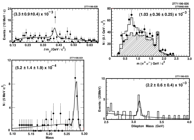
Figure 20: Plots of three wrong and one correct result. The results and the errors are quoted on each plot. References are deliberately not provided. The correct plot that is showing a real signal is listed in the text.

The point of showing this figure is that it is not at all obvious by looking at the plots which is right or wrong. One needs to examine the individual analyses in more detail. It is important to ask: What are the pitfalls? Where do experimenters make mistakes? How can you tell?

In two of the flawed results of Figure 20, my personal opinion is that the selection cuts for a signal were tuned on the data instead of on MC. In a third result, the mistake was, I believe, a large background that the experimenters assumed the MC modeled properly and it didn’t.

The correct result is the top left plot of Figure 20 and I have deliberately shown the worst looking plot from the analysis. The result can be made to look much better with different binning. That is considered cheating if it affects the signal yield extracted by the analysis. In this particular analysis, the yields were computed with very fine binning and it was tested that they were independent of bin size. The evaluation of the background was done many different ways (from data and MC ) and the result was stable when the cuts were changed. These are all checks you should expect to see experimenters do.

So what are the questions you should ask when deciding whether to believe a marginal (3–4 $\sigma$) result or in deciding whether you believe the level of precision on a more significant result?

1. How were event selection criteria determined?

2. How was the background evaluated?

3. What happens when the event selection cuts are varied?

4. What is the error on the efficiency and how was it determined?

There are some other pitfalls you should be aware of:

• Sometimes experimenters do not understand their detectors as well as they think they do. This is evident if one looks at the high resolution measurments of the $B$ meson lifetime as a function of time $\!{}^{{\bf?}}$ starting in 1986 as shown in Figure 21. The $B$ lifetime has increased by almost 50% of its value as increasingly precise detectors have been used and larger data sets have been analyzed. Some of the early results were optimistic about their error bars and the systematic shift has presumably resulted from improvements in the analysis procedures and a better understanding of the detectors.

  

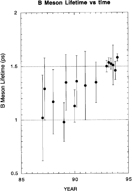
  Figure 21: The measured $B$ meson lifetime as a function of time.

• Experimentalists and theorists alike are prone to over-averaging, where many measurements are averaged, weighted by their combined statistical and systematic error. The Particle Data Group, a wonderful institution in every respect, contributes to this problem in some ways by making the data so easily available.

  A famous example of over averaging was the “$\tau$ 1-prong problem.” The $\tau$ lepton can decay just like the muon ($\tau\to e\nu\bar{\nu}$, $\tau\to\mu\nu\bar{\nu}$), but it can also decay to hadrons. In 1984, it was noticed that if one took the world averages for the measured $\tau$ branching ratios and used theoretical predictions to constrain poorly measured modes, then the measured inclusive 1-prong branching ratio was significantly larger than the sum of the exclusive modes. $\!{}^{{\bf?}}$ As late as 1992, one saw that, taking world averages, one found a significant discrepancy in the inclusive rate and the sum of the exclusive rates. $\!{}^{{\bf?}}$

  For years there were speculations about new physics and unseen decay modes. The problem, however, was caused by averaging many experiments with large errors and extracting an average with rather small errors. It is very dangerous to take results from 10 different measurements with roughly equal precision and then average them to get a factor of three smaller error. If errors were statistical only, there would not be a difficulty. The problem comes from systematic errors which may be correlated experiment to experiment. Systematic errors are hard to evaluate to begin with, and correlations are hard to spot. For example, there may be unknown correlated errors due to incorrect inputs to the MC or overlooked backgrounds. The moral is that global averages need to be done with great care and even then, I believe that one needs to use a higher threshold for claiming a significant discrepancy when averaged data is being used.

• A third pitfall that affects experimenters more than theorists, but you should be aware of it, is the enormous temptation to stop at the “right answer”. Certainly anyone who has ever done a freshman physics lab knows that feeling. We very often have a preconceived prejudice on what a result should be. A good experimenter does many of the systematic studies and checks before looking at the actual number he or she is getting.

• Finally, theorists tend to fall into the “single event” pit. What does it mean to find a single event? In 1964, the $\Omega^{-}$ was discovered with the observation of one event. $\!{}^{{\bf?}}$ However, there was an enormous amount of information in the bubble chamber photograph that captured that one event. The decay was fully reconstructed $K^{-}p\to\Omega^{-}K^{+}K^{0},\Omega^{-}\to\Xi^{0}\pi^{-},\Xi^{0}\to\Lambda^{0}\pi^{0},\Lambda^{0}\to\pi^{-}p,\pi^{0}\to\gamma_{1}\gamma_{2},\gamma_{1}\to e^{+}e^{-},\gamma_{2}\to e^{+}e^{-},$ except for the $K^{0}$. They were able to claim discovery because there was so much information in the event that the probability for the background to produce such an event was vanishingly small. However, for modern collider experiments, it is impossible to have the same level of information, especially in $p\bar{p}$ collisions where much of the event goes down the beam pipe. The crucial issue is not how many events one finds, but how well the background can be evaluated and understood, and what is the probability that a background process could imitate the event one is looking for.

4 Measuring Parameters of the Standard Model

In Section 2, I listed the parameters of the Standard Model that must be determined experimentally. I will spend this section discussing some of those experiments. I like to think of them as the measurements that define the Standard Model.

4.1 Measurements of Coupling Constants

I will start with a description of how to measure a coupling constant. The coupling constants in the SM are $\alpha_{\rm EM},\alpha_{s}$ and $G_{F}$. The most precise determination of $\alpha_{\rm EM}$ comes from the electron $g-2$ experiments using single trapped electrons $\!{}^{{\bf?}}$:

$$\alpha_{EM}^{-1}=137.035\ 992\ 35\ \left(73\right)$$ (18)

$G_{F}$ is determined from the muon mass and lifetime using the relation:

$$\frac{1}{\tau_{\mu}}=\frac{G_{F}^{2}M_{\mu}^{5}}{192\pi^{3}}$$ (19)

and the dominant uncertainty on $G_{F}$ comes from the second order radiative corrections to this expression $\!{}^{{\bf?}}$, and the result is:

$$\frac{G_{F}}{\left(hc\right)^{3}}=1.16639\left(2\right)\times 10^{-5}{\rm GeV}^{-2}$$ (20)

$\alpha_{s}$ is the most poorly measured quantity in the entire physical constants list of the Particle Data Group $\!{}^{{\bf?}}$:

$$\alpha_{s}(M_{Z})=0.116(5)$$ (21)

There is some theoretical uncertainty over how best to determine $\alpha_{s}$; I expect lots of progress here in the next few years.

I want to talk briefly about how $\alpha_{s}$ is measured. There are many different techniques that are employed at different $Q^{2}$ as shown in Figure 22, and the remarkable agreement between them is considered one of the great successes of QCD $\!{}^{{\bf?}}$.

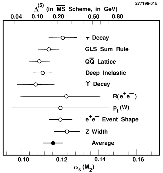
Figure 22: A plot of the value of $\alpha_{s}$ as measured in a variety of experiments at different $Q^{2}$. All measurements have been evolved to $\alpha_{s}(M_{Z})$ for comparison purposes.

The most obvious way to measure a coupling constant of a particular interaction is to measure the energy spectrum of the system bound by that interaction. For example, in the early days of quantum mechanics, the Rydberg was measured from the spectrum of atomic hydrogen. Similarly, one uses the spectroscopy of a system bound by the strong interaction to measure $\alpha_{s}$. This procedure has a slight difficulty. For QED, the interaction that binds the $e^{-}$ in the hydrogen atom, we can write down the Schrodinger equation and solve it to get the relation between the measured energy levels and the coupling constant of the interaction. For QCD it is not so easy; there is no equivalent to the Schrodinger equation for the strong interaction. However, QCD is being solved with lattice techniques, allowing us to relate $\alpha_{s}$ to the measured energy splittings $\!{}^{{\bf?}}$.

One of the bound state systems used for the $\alpha_{s}$ extraction is the $\Upsilon$ system (a bound state of a $b$ and a $\bar{b}$ quark). The mass of the $b$ quark is around 5 GeV. Between the energies of 9.46 and 11 GeV, the spectrum of $b\bar{b}$ quark bound states is rich. In an $e^{+}e^{-}$ machine such as CESR, the bound states with the same quantum numbers as the photon are copiously produced and show up as dramatic features in a scan of hadronic cross section versus CM energy as shown in Figure 23.

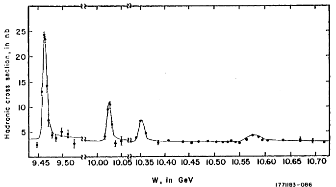
Figure 23: A scan of the hadronic cross section versus energy in the $\Upsilon$ energy region from CLEO showing the $b\bar{b}$ bound states.

The experiment is easy to do. One scans the energy of the $e^{+}e^{-}$ beams and looks at the number of events in the detector, where an event is loosely defined as three or more tracks.

There is an underlying continuum of $e^{+}e^{-}\to\gamma^{*}\to q\bar{q}$ events. Then there is a dramatic increase in the number of events observed when producing the ${}^{3}S_{1}$ states of the $b\bar{b}$ bound state system. The observed resonances are the $n=1,n=2,n=3$, and $n=4$ radial excitations. The low-lying resonances are narrow because their decays, which are dominantly three gluon exchange, are suppressed. The ${}^{3}S_{1}$, $n=4$ radial excitation is wide because it is massive enough to be fully allowed to strongly decay to a pair of $B$ mesons.

From the energy of the $e^{+}e^{-}$ beams, we get the energies of the $\Upsilon$ states. Other bound states of the $b\bar{b}$ system are observed by seeing pion or photon transitions from the ${}^{3}S_{1}$ states. Similar studies are performed on the $c\bar{c}$ bound states such as the $J/\Psi$. By fitting the energy levels, one gets $\!{}^{{\bf?}}$

$$\alpha_{s}\left(M_{Z}\right)=0.110\left(6\right)$$ (22)

where it is convention to evolve $\alpha_{s}$ from the $Q^{2}$ where it is measured up to $M_{Z}$ using the renormalization group equations. The errors are dominated by the systematics of the lattice calculation: a finite lattice spacing is used and the quenched approximation is made, where no light quarks are allowed to propagate.

Other ways exist to measure $\alpha_{s}$. In almost all other methods, the measurement is sensitive to $\alpha_{s}$ as a radiative correction. As an example,

$$R=\frac{\sigma\left(e^{+}e^{-}\to{\rm hadrons}\right)}{\sigma\left(e^{+}e^{-}\to\mu^{+}\mu^{-}\right)}$$ (23)

can be used to measure $\alpha_{s}$. You have all calculated the cross section for $e^{+}e^{-}\to\mu^{+}\mu^{-}$

$$\sigma_{\mu^{+}\mu^{-}}=\frac{4\pi\alpha_{EM}^{2}}{3s},\qquad s=E_{CM}^{2}$$ (24)

For $e^{+}e^{-}\to q\bar{q}$ the $\mu$ charge ($e$) is replaced by $Q|e|$ and you get an extra factor of 3 for 3 quark colors.

$$\sigma_{q\bar{q}}=\frac{4\pi\alpha_{EM}^{2}}{3s}Q_{i}^{2}\times 3$$ (25)

Naively, then, $R=3\cdot\sum Q_{i}^{2}$ since the quarks will make hadrons 100% of the time. However, the expression for $R$ is modified by higher order QCD corrections to be

$$R=R^{\left(0\right)}\left[1+\frac{\alpha_{s}}{\pi}+....\right]$$ (26)

and so by careful experimental measurements of $R$ one can extract $\alpha_{s}$.

At the moment theoretical errors dominate in virtually all measurements of $\alpha_{s}$.

4.2 Measurements of a Gauge Boson Mass

Once $G_{F}$ and $\alpha_{EM}$ are measured, we need one more experimental quantity to define the SM, and then all other measurements of fermion couplings, $W$ mass, and so on, will constitute checks of the model. We need to determine either a gauge boson mass ($M_{Z},M_{W}$) or a weak mixing angle ($\sin^{2}\theta_{W}$) from deep inelastic scattering or atomic physics. We want to use the most precise quantities available to define the model. Ever since the precision LEP measurements of the $Z$ mass, $M_{Z}$ has become the third parameter of choice.

In principle and in practice, you can measure $M_{Z}$ in either $e^{+}e^{-}$ or $p\bar{p}$ collisions. In $p\bar{p}$ collisions, there is a broad spectrum of incoming parton energies and the initial state energy is not known. However, one can use the clean leptonic decays $Z\to e^{+}e^{-},\mu^{+}\mu^{-}$ to select background-free samples of events, and from a measurement of the momentum vectors of the final state particles (typically with few percent resolutions), one can reconstruct the invariant mass of the parent boson and determine $M_{Z}$.

In $e^{+}e^{-}$ collisions, the CM annihilation energy is well known. The machine energy spread (the energy spread of the electron and positron beams) is much less than the width of the resonance. One can study the resonance shape directly. There is very little background and these experiments have the highest precision.

The cross section to produce $Z$’s at the pole is large (30 nb). A machine like LEP can produce thousands of $Z$’s per day and the very large data samples have made detailed studies of all the decays of the $Z$ possible. It is again straightforward to calculate $\sigma\left(e^{+}e^{-}\to Z^{0}\to f\bar{f}\right)$ in the SM $\!{}^{{\bf?}}$. At the $Z$ pole, the contribution to $\sigma\left(e^{+}e^{-}\to f\bar{f}\right)$ from QED is negligible.

$$\sigma_{\rm pole}\left(e^{+}e^{-}\to Z^{0}\to f\bar{f}\right)=\frac{G_{F}^{2}M_{Z}^{4}s\left(R_{e}^{2}+L_{e}^{2}\right)}{24\pi\left[\left(s-M_{Z}^{2}\right)^{2}+M_{Z}^{2}\Gamma_{Z}^{2}\right]}\left(R_{f}^{2}+L_{f}^{2}\right)$$ (27)

Here, $R_{e}$ and $L_{e}$ are the right and left handed electron couplings to the $Z$, $R_{f}$ and $L_{f}$ are the right and left handed fermion couplings to the $Z$, and $\Gamma_{Z}$ is the total width of the resonance. This is often expressed using

$$\sigma_{0}^{f\bar{f}}=\sigma\left(\sqrt{s}=M_{Z}\right)=\frac{G_{F}^{2}M_{Z}^{4}}{24\pi\Gamma_{Z}^{2}}\left(R_{e}^{2}+L_{e}^{2}\right)\left(R_{f}^{2}+L_{f}^{2}\right)$$ (28)

which then gives:

$$\sigma_{\rm pole}\left(e^{+}e^{-}\to Z^{0}\to f\bar{f}\right)=\sigma_{0}^{f\bar{f}}\frac{s\Gamma_{Z}^{2}}{\left[\left(s-M_{Z}^{2}\right)^{2}+M_{Z}^{2}\Gamma_{Z}^{2}\right]}$$ (29)

$M_{Z}$ determines the location of the Breit-Wigner resonance, $\Gamma_{Z}$ determines the width, and $\sigma_{0}$ determines the normalization. In fact, only one free parameter is needed to fit the $Z$ line shape: $M_{Z}$. The SM predicts the values of $\Gamma_{Z}$ and $\sigma_{0}$ in terms of $M_{Z}$. Initially, however, one fit the resonance to three independent parameters, $\sigma_{0},\Gamma_{Z},$ and $M_{Z}$ to check the model for consistency.

It is impossible to go further in our discussion of $M_{Z}$ without a discussion of radiative corrections. In the study of the $Z$ resonance, there are two types of radiative corrections.

• QED radiative corrections: here real photon emission from an initial state $e^{+}$ or $e^{-}$ occurs. It is a dramatic effect, and does not contain any particularly new or interesting physics.

• EW radiative corrections: these come in as vacuum polarization and vertex corrections to the tree level process $e^{+}e^{-}\to Z^{0}\to f\bar{f}$. These corrections affect the tree level relations between $\alpha_{EM},G_{F},M_{Z}$ and $M_{W},\sin^{2}\theta_{W}$ derived from other experiments.

QED Radiative Corrections

When you tune $e^{+}e^{-}$ beams to a particular CM energy, you want to measure the cross section at that energy. In fact, however, you may be sampling the cross section at some other lower energy because bremsstrahlung from the incoming $e^{+}$ or $e^{-}$ has removed energy from the CM. In an experiment, one actually samples the entire cross section below the nominal CM energy with a sampling spectrum $f\left(k\right)$ that is determined by the physics of bremsstrahlung.

$$\sigma_{\rm obs}\left(E\right)=\int dkf\left(k\right)\sigma_{\rm BW}\left[E\left(E-k\right)\right]$$ (30)

There are two reasons that this becomes a large effect at the $Z$ resonance.

1. The amplitude for single photon emission from the electron or positron can be written in terms of the annihilation amplitude with no photon emission as:

   $$a_{1\gamma}=e\left(\frac{p^{+}\cdot\epsilon}{k\cdot p^{+}}-\frac{p^{-}\cdot\epsilon}{k\cdot p^{-}}\right)a_{0\gamma}$$ (31)

   where $k$ is the photon 4-vector, $p^{\pm}$ refers to the electron and positron 4-vector, and $\epsilon$ is the photon polarization. Summing over photon polarization and integrating over photon angles we get the change in the cross section due to initial state radiation:

   $$d\sigma=\sigma_{0}\left(s\right)\left[\frac{2\alpha_{EM}}{\pi}\left(\ln\frac{s}{m_{e}^{2}}-1\right)\right]\frac{dk}{k}$$ (32)

   where the term in the square brackets is often call $\beta$, the “effective coupling” for bremsstrahlung. $\beta$ is large ($\ln\frac{s}{m_{e}^{2}}=24.2$ at the $Z$ resonance and $\beta=10\%$) due to the large phase space for an $e^{-}$ to shake off a nearly collinear photon.

2. To get the cross section, we integrate $d\sigma$ (to do this right we need to include vertex corrections to remove infrared divergences as $k\to 0$.)

   $$\int_{0}^{k_{\rm max}}d\sigma=\sigma_{0}\left(s\right)\left[1+\delta_{1}+\beta\ln\frac{k_{\rm max}}{E}\right]$$ (33)

   where $\delta_{1}$ is often called the first order $e^{-}$ form factor.

   To evaluate this expression, we need $k_{\rm max}$. In general bremsstrahlung energies can extend up to the kinematic limit which is the beam energy, but when one is sitting on a narrow resonance, if the initial state radiation is much more than the width of the resonance, one is moved into a region of very low cross section. Therefore, the resonance cuts off contributions from hard photons which in effect puts an upper limit $k_{\rm max}\sim\Gamma/2$.

   $$\sigma\left(M_{Z}^{2}\right)=\sigma_{0}\left(M_{Z}^{2}\right)\left(1+\delta_{1}+\beta\ln\frac{\Gamma}{M}\right)$$ (34)

   The narrow resonance cuts off contributions from all but the softest radiative events, depressing the cross section significantly ($\beta\ln\frac{\Gamma}{M}\sim-39\%$ at the $Z$), and the resonance shape is skewed by a high energy tail.

The stunning fact is that it was only in 1987 that the second order calculations of these QED radiative corrections were completed; just in time for LEP and SLC. $\!{}^{{\bf?}}$

EW Radiative Corrections

At tree level in the Standard Model, we measure $\alpha_{EM},G_{F},M_{Z}$ and from them we can calculate $M_{W}$ and $\sin^{2}\theta_{W}$. We can then check the Standard Model by measuring $M_{W}$ or $\sin^{2}\theta_{W}$ directly. Unfortunately, life is not lived at tree level, and when we measure the $Z$ mass, we really measure the sum of the tree level process and all the radiative corrections to it. Nature has summed the perturbation series for us. One effect of these higher order corrections is that coupling constants run and their values change with $Q^{2}$. For example, in QED:

$$\alpha_{\rm EM}\left(q^{2}\right)=\frac{\alpha_{EM}}{1-\frac{\alpha_{EM}}{3\pi}\ln\frac{q^{2}}{m^{2}}}$$ (35)

One way to think of this renormalization of the electron charge is that it comes from the static polarizability of the vacuum. At higher values of $q^{2}$, one is probing shorter distances, getting closer to the bare charge which is infinite. As experimentalists, we are lucky that nature (correctly) has computed all the radiative corrections for us to all orders. The problem is that the radiative corrections will modify the simple tree level relations between, for example, $G_{F}$ and $\sin^{2}\theta_{W}$ or $\sin^{2}\theta_{W}$ and $M_{W}$.

Consider the following two definitions of $\sin^{2}\theta_{W}$. They are equivalent at tree level:

$$\sin^{2}\theta_{W} = 1-\frac{M_{W}^{2}}{M_{Z}^{2}}$$ (36)

$$\sin^{2}\theta_{W} = \sqrt{\frac{4\pi\alpha_{EM}}{\sqrt{2}G_{F}M_{Z}^{2}}}$$ (37)

where in both expressions, the physical boson masses are used, and in the second expression, $\alpha_{EM}$ and $G_{F}$ are determined from low energy experiments. These two relations, while equivalent at tree level, will give different results when experimental data are used.

We can parameterize the effect of the radiative corrections by a correction to our relations. We can define $\sin^{2}\theta_{W}$ from the physical boson masses as:

$$\sin^{2}\theta_{W}\equiv 1-\frac{M_{W}^{2}}{M_{Z}^{2}}$$ (38)

Then equation  37 is modified:

$$\sin^{2}\theta_{W}=\sqrt{\frac{4\pi\alpha_{EM}}{\sqrt{2}G_{F}M_{Z}^{2}\left(1-\delta r\right)}}$$ (39)

where $\delta r$ incorporates the effects of the radiative corrections. The largest contribution to $\delta r$ is just from the running of $\alpha_{EM}$ to the $Z$ mass.

$$\alpha_{EM}\left(M_{Z}^{2}\right)=\left[128.8\pm 0.12\right]^{-1}$$ (40)

and the next largest contribution to $\delta r$ comes from the top quark which gives a contribution:

$$\delta r_{t}=-\frac{3G_{F}m_{t}^{2}}{8\sqrt{2}\pi^{2}}\frac{1}{\tan^{2}\theta_{W}}\simeq-0.0102\left[\frac{m_{t}}{100{\rm GeV}/{\rm c}^{2}}\right]^{2}$$ (41)

which gives a 3% correction for $m_{t}\simeq 175$ GeV/c².

The fact that the radiative corrections to the electroweak observables are sensitive to the top quark mass means that precision measurements of the radiative corrections can be used to determine the top mass. If one assumes that the SM is correct and there is no new physics, then a combination of a measurement of $\alpha_{EM},G_{F}$, and $M_{Z}$ with one other precise measurement (i.e., $\sin^{2}\theta_{W}$ extracted from a measurement of quark or lepton couplings to the $Z$) gives a “measurement” of $m_{t}$! Before the top quark was discovered, LEP provided a tight ($\pm 15\%$) constraint on its mass in just this fashion $\!{}^{{\bf?}}$.

Experimental measurement of the $Z$ mass

The precision measurement of the $Z$ mass comes from LEP. LEP is an electron positron collider, 26.66 km in circumference, capable, ultimately, of almost 100 GeV/beam. To measure the $Z$ mass, one scans the energy of the machine through the $Z$ resonance. The number of events of the types $Z^{0}\to$ hadrons, $e^{+}e^{-},\mu^{+}\mu^{-},\tau^{+}\tau^{-}$ in the detector are counted. A plot of the number of events versus energy, such as is shown in Figure 24, is fit to extract $M_{Z}$.

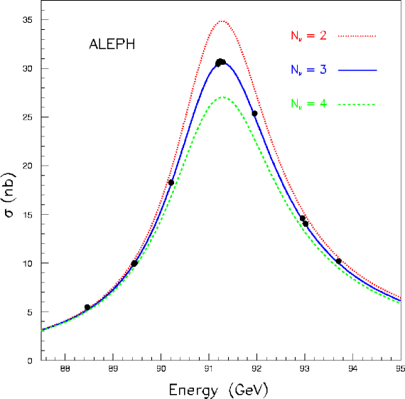
Figure 24: A scan of the $Z$ resonance taken by ALEPH. The three curves indicate the expected lineshape for 2, 3 and 4 flavors of light neutrinos. (http://www.cern.ch/ALEPHGENERAL/reports/figures/ew/zline aleph.gif)

The precision of the measurement depends crucially on the absolute energy calibration of the machine. LEP uses a resonant spin depolarization technique with an intrinsic accuracy of $\sim 1$ MeV to determine the absolute energy scale of the machine during special experimental runs. This calibration then must be transferred from 2 GeV above the $Z$ resonance where the calibration experiment is done to the energies of the scan points for the mass measurement. In practice, LEP achieves a systematic error of $\pm 3.7$ MeV for the absolute beam energy. In attempting to improve the systematic error, studies have shown that the energy of the LEP machine is sensitive to the tides, the lake levels, the magnet temperature, and, most recently, they have found a correlation between the voltage on the TGV and the energy of the LEP beam at the MeV level! For the $Z$ mass measurement, LEP quotes an uncertainty on the absolute beam energy calibration $\!{}^{{\bf?}}$ of $\sigma_{E}/E=5.3\times 10^{-5}$, and from the scan to the $Z$ resonance they find: $M_{Z}=91.179\pm 0.007$GeV/c². $\!{}^{{\bf?}}$

4.3 Measurements of a Yukawa Coupling

Next on the list of Standard Model parameters to measure is a fermion mass, or if you prefer, a Yukawa coupling. The masses of all the fermions have been measured (or in the case of the neutrinos, upper limits have been set on their masses with a possible lower limit coming from LANL observation of $\nu$ oscillations $\!{}^{{\bf?}}$). The masses of charged leptons are determined quite precisely but the masses of quarks are less well known due to the complications of the strong interactions. The masses are listed in Table 3 $\!{}^{{\bf?}}$.

Table 3: Masses of the known fermions in MeV/c².

$m_{e}$ = 0.51099906(15)	$m_{\nu_{e}}$ $<7\times 10^{-6}$
$m_{\mu}$ = 105.658389(34)	$m_{\nu_{\mu}}$ $<0.27$
$m_{\tau}$ = $1771.1^{+0.4}_{-0.5}$	$m_{\nu_{\tau}}$ $<31$
$2<m_{u}<8$	$5<m_{d}<15$
$10^{3}<m_{c}<1.6\times 10^{3}$	$10^{2}<m_{s}<3\times 10^{2}$
$m_{t}=(1.76\pm 0.16)\times 10^{5}$	$4.1\times 10^{3}<m_{b}<4.5\times 10^{3}$

I will discuss the recent measurement of the top quark mass as an example of how to measure a Yukawa coupling. Note that this is quite unique among the fermion mass measurements: the top quark is the highest rest mass particle ever observed!

To measure the top quark mass, you must first discover the top quark! Actually, this is not true. The constraints on the top mass from the electroweak radiative corrections measured at the $Z$ pole were quite impressive. Before the top quark was discovered, Langacker and Erler $\!{}^{{\bf?}}$ found $m_{t}=169\pm 24$ GeV/c²; however, lots of assumptions go into that “measurement.” The basic assumption is that there is nothing else new in the Standard Model beyond what we already know. However, I want to talk about the measurement of the top quark mass from the reconstruction of its decay products.

With the mass of the top quark so high, the only machine capable of producing $t$ is the Tevatron. Top quarks are produced in $p\bar{p}$ collisions by three main mechanisms illustrated in Figure 25:

• $t\bar{t}$ pair production

• single $t$ production via Drell-Yan

• single $t$ production in $W$-gluon fusion.

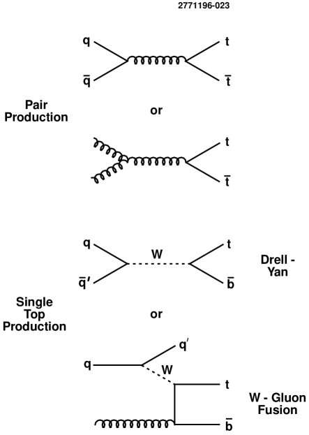
Figure 25: The dominant top quark production mechanisms at FNAL: $t\bar{t}$ pair production, single $t$ production via Drell-Yan, and single $t$ production in $W$-gluon fusion.

At FNAL, for a high top quark mass, production is dominated by $t\bar{t}$ pair production.

The dominant decay of top is to $Wb$ followed by $W\to\ell\nu,u\bar{d},$ or $c\bar{s}$. There will be two $b$ quarks and 2 $W$’s in each event. There are two classes of $t\bar{t}$ events that can be reconstructed: the first class is where both $W$’s decay leptonically to electrons or muons (5% of all decays), and the second class is where one $W$ decays leptonically to an electron or a muon and the other $W$ decays to two jets (30% of all decays). For the initial discovery of top, both channels were used. However, for the mass measurement, only a subset of the events was used. The reason is that in the case where both $W$’s decay leptonically, the system is underconstrained for the mass measurement since there are two missing neutrinos in the event. I will concentrate on describing the selection of $t\bar{t}$ events in the lepton and jets channel, which is illustrated in Figure 26, since these are the events used for the mass measurement $\!{}^{{\bf?}}$.

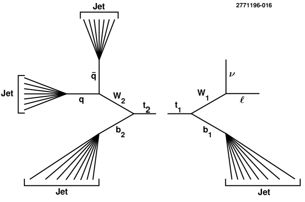
Figure 26: A schematic view of the lepton plus jets decay mode of the two top quarks produced at FNAL energies. This is the channel used in determining the top quark mass at CDF.

A standard way to measure a particle mass is to measure the momenta of all of the decay products and then reconstruct the invariant mass of the parent particle. For the top search, the implementation of this procedure is not obvious. For events in which

$$t_{1}\to W_{1}b_{1},\qquad W_{1}\to\ell\nu\qquad t_{2}\to W_{2}b_{2},\qquad W_{2}\to q\bar{q}$$ (42)

the momentum and energy of the lepton can be measured in a straightforward fashion. The measurement of the momenta and energies of the quarks is hard. This would all be much simpler if we could detect quarks, but we cannot. Quarks hadronize, making clusters of particles in the detector called jets. The jet energy resolution is poor, there can be gluon radiation giving extra jets in the event, and the combinatorics are not favorable as there are 24 ways of assigning the four jets detected to the four final state quarks. Fortunately one can require one of the jets to be a $b$ jet in order to reduce combinatorics. The field of jet spectroscopy is in its infancy. As we go to higher energy machines, we will have to get better at it!

With the jet and lepton 4-vectors in hand there are three constraints to calculate the remaining unknown neutrino 4-vector:

• $M\left(q\bar{q}\right)=M_{W}$

• $M\left(\nu\ell\right)=M_{W}$

• $m\left(t_{1}\right)=m\left(t_{2}\right)$

Events for the $t$ mass measurement in CDF are selected by requiring one hard lepton and four or more jets. CDF requires that one jet in the event have a $b$-tag: either there is a separated vertex consistent with the finite $b$ lifetime, or a soft lepton consistent with coming from a $B$ meson decay. After the $b$-tag, CDF has a sample of 19 events,where approximately 6 are estimated to come from background.

The top quark mass is calculated using the information from the constrained fit. If the jets are correctly assigned, the resolution on the mass is $\approx 12$GeV/c². Because of gluon radiation and incorrect assignments, the resolution is in practice $\approx 24$GeV/c². The CDF distribution of invariant mass formed from decay products is shown in Figure 27 and gives $m_{t}=176\pm 8\pm 10$, where the systematic error is determined by the uncertainty in the response of the calorimeter to hadrons giving an uncertainty in the jet energy scale, and the uncertainty in the underlying QCD processes that form the jets $\!{}^{{\bf?}}$.

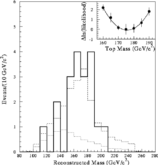
Figure 27: The reconstructed mass distribution of the top quark from CDF. The solid line is the data. The dotted line is the background shape, and the sum of the background and $t\bar{t}$ Monte Carlo is the dashed line.

The top mass measurement is among the first examples of using jet spectroscopy to determine the mass of a particle. We can expect to see this technique improved and exploited at future machines.

4.4 Measuring a Mixing Angle

The final experiment I want to discuss is how to measure a quark mixing angle. Recall that the quark eigenstates of the strong interactions, which are the states of definite flavor, are not eigenstates of the weak interactions. In quantum mechanical terms, flavor is a symmetry of the strong interactions, so the strong interaction is diagonal on the quark flavor basis ($u,c,t,d,s,b$). However, the weak interaction is diagonal on a different basis ($u,c,t,d^{\prime},s^{\prime},b^{\prime}$) and there is some unknown and undetermined rotation matrix that relates the two bases. It is up to experiment to determine the elements of the $3\times 3$ rotation matrix. The effect of the flavor mixing is that the strength of the weak interaction between two quark states of definite flavor will be modified by a coefficient from this rotation matrix to account for the flavor mixing. For example, the strength (and hence the rate) of $b$ to $c$ decay will be modified by an unknown factor we will call $V_{cb}$. By measuring the decay rate, we can extract $V_{cb}$.

Figure 28 gives a summary of the CKM matrix and how the elements are measured $\!{}^{{\bf?}}$. The values quoted are what are actually measured. The requirement that the matrix be unitary provides a powerful constraint on the poorly measured elements.

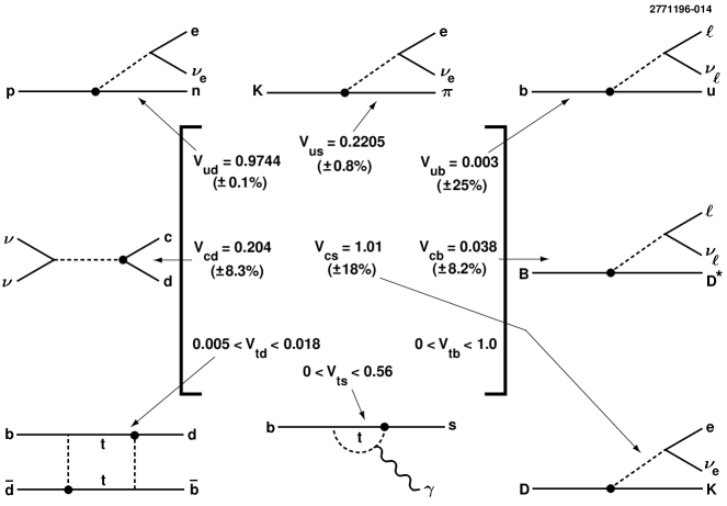
Figure 28: The measured values of the CKM matrix elements and a schematic indication of the processes used to measure them.

As an example, I will discuss a measurement of $V_{cb}$ by the CLEO detector using $B$ mesons produced by CESR. Let me remind you that CESR is an electron-positron storage ring with a center of mass energy $E_{CM}=10.58$GeV. At that energy, one is just above threshold to produce a pair of $B$ mesons and nothing else.

The strategy for the measurement is to use the decay $B\to D^{*}\ell\nu$. In Section 3.4, I discussed briefly how to select the event sample, evaluate backgrounds and efficiencies, and measure the rate for the decay. Recall that experimentally, we measure a branching ratio which is related to the decay rate by the relation:

$$\Gamma\left(B\to D^{*}\ell\nu\right)=\frac{{\rm BR}\left(B\to D^{*}\ell\nu\right)}{\tau_{B}}$$ (43)

We use Fermi’s golden rule to relate the measured decay rate to the underlying physics:

$$\Gamma_{B\to D^{*}\ell\nu}=\frac{2\pi}{\hbar}|<D^{*}\ell\nu|V_{cb}{\cal H}|B>|^{2}\rho\left(E\right)=\kappa V_{cb}^{2}$$ (44)

We need to evaluate the matrix element (overlap integral) in order to get the constant of proportionality between $\Gamma$ and $V_{cb}$ and here we run into trouble because we cannot solve the Schrodinger equation for the $B$ meson. We do not know what wave functions to put in for the mesons in order to calculate the matrix element. For years, theorists have made educated guesses for meson wave functions and generated calculations for $\kappa$. For educated guess read systematic error on $V_{cb}$! Now, however, there is a better way. This is an example of an area where the developments in theory and experiment go hand in hand.

A new theoretical approach to calculating the form factors or overlap integrals for exclusive semileptonic decays has attracted a lot of attention in recent years. The basic idea is to notice that a $B$ meson or a charm meson (in both cases a light quark bound to a very heavy quark) looks a lot like the hydrogen atom, which is a light $e^{-}$ bound to a heavy proton. This approach is called heavy quark effective theory (HQET) $\!{}^{{\bf?}}$. What can it buy in the extraction of CKM matrix elements? Recall that the $e^{-}$ wave function in the hydrogen atom is independent of the mass and spin of the proton, up to hyperfine corrections. We might guess that the light quark part of the meson wave function should be independent of the mass of the heavy quark up to hyperfine corrections of order $\Lambda_{QCD}/m_{Q}$, where $m_{Q}$ is the mass of the heavy quark, and, like the proton in the H atom, the heavy quark should behave like a free particle.

The implication of the two previous statements is that the meson wave function should factorize and therefore so does the matrix element. When one calculates the amplitude for this decay, there is a heavy quark part describing the decay of a free $b$ quark to a free $c$ quark, which is calculable, and there is a light quark overlap integral describing the probability for the light quark cloud in the initial state to turn into the light quark cloud in the final state. This overlap integral depends on the velocities of incoming and outgoing mesons, and is not calculable from first principles.

However, the light quark overlap integral is universal. It should be the same for all heavy pseudoscalar or vector meson to heavy pseudoscalar or vector meson decays. It is called the Isgur-Wise function: $\xi(v\cdot v^{\prime})$. All of the form factors for $B\to D,D^{*}\ell\nu$ decays can be written in terms of $\xi$. It is a help that now there is only one unknown in the problem that needs to be modeled, but this is still an experimentally unsatisfactory situation since we know nothing about $\xi$.

What makes HQET attractive is that at zero recoil, when the initial and final state mesons are at rest, $\xi\left(v\cdot v^{\prime}=1\right)=1$, the form factors describing the overlap of the initial and final light quark wave functions are absolutely normalized. This absolute normalization is the result of the fact that at zero recoil, since the light quark wave function is independent of the mass of the heavy quark, the light quark does not know a $c$ quark has replaced a $b$ quark. There is no velocity mismatch and the overlap is perfect. At this magic kinematic point, you can measure $V_{cb}$ independent of any unknown form factor. Perhaps a simpler way of saying it is one can trade statistics in data to measure the decay rate in a corner of phase space where the form factor is well known.

HQET is only an approximation. There are corrections to it. By a stroke of good fortune, the point of zero recoil is protected from first order corrections in $\Lambda_{QCD}/m_{Q}$ and we need only worry about second order effects. We can extract $V_{cb}$ from $B\to D^{*}\ell\nu$ taking advantage of HQET by plotting the differential branching ratio as a function of $y=v\cdot v^{\prime}$. HQET says that at zero recoil ($q_{\rm max}^{2}$ or $y=1$) the form factor is 1, up to hyperfine corrections. Therefore, when properly normalized, the intercept of the differential decay rate at $y=1$ yields $V_{cb}$. To determine the intercept, the data are extrapolated from $q^{2}<q_{\rm max}$, using a linear expansion of the Isgur Wise function as shown in Figure 29. From this analysis, we find $\!{}^{{\bf?}}$ $|V_{cb}|=0.0362\pm 0.0019\pm 0.0024$.

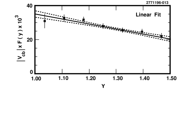
Figure 29: The differential decay distribution for $B\to D^{*}\ell\nu$ decays from CLEO. The left intercept yields $V_{cb}$.

I would like to point out that to many people, form factor calculations may seem to simply be grubby phenomenology, but in the extraction of the CKM matrix elements, we are in most cases limited by our understanding of the hadronic matrix elements in our determination of these fundamental parameters of the Standard Model!

5 Testing the Standard Model

5.1 The Search for the Higgs

There is one final element that we need in order to define the SM and it will also provide us with a profound test of the model. In its simplest versions, the SM predicts – in fact requires – the existence of a neutral scalar particle: the Higgs boson. The observation of the Higgs is the most important prediction of the SM that has not yet been verified by experiment. It is a challenge to search for the Higgs because while the coupling of the Higgs to the fermions and gauge bosons is now completely determined by the experiments we have discussed so far, we have no prediction of the Higgs mass from the theory. It is hard to design experiments to search for the Higgs, since they must be sensitive to all masses!

In practice, the search is not so difficult as it might at first seem. The pre-LEP experiments were able to rule out different chunks of the mass range. The LEP I experiments $\!{}^{{\bf?}}$ were able to eliminate a Higgs with $0\leq M_{H}\leq 58.4$ GeV/c² and LEP II will extend that limit (assuming they don’t find the Higgs) to almost 100 GeV/c².

There is another aspect of the Higgs search that needs discussing. There are very few in the high energy community who believe that the minimal Standard Model is a fully satisfactory and complete description of nature. The model contains many arbitrary parameters and the mechanism for giving mass to the fermions is totally ad hoc. There is a sense that there must be something more. As a result, most high energy physicists view the search for the Higgs not as a final nail in the coffin (once the Higgs is found and its mass measured, then we have a complete theory) but rather the search for the Higgs is the most likely gateway to really new physics.

There is an excellent discussion in the text of Peskin and Schroeder $\!{}^{{\bf?}}$ that asks whether the $W$ and $Z$ might have acquired their mass by some different, more complicated mechanism than spontaneous symmetry breaking, since there is no experimental evidence for the Higgs. Peskin and Schroeder argue that there is compelling experimental evidence that the underlying theory of the weak interactions is a spontaneously broken gauge theory. There is no other principle except for a spontaneously broken gauge theory that could explain the experimental observation of universal, flavor-independent coupling constants that describe the entire range of neutral current phenomena. However, they point out that the mechanism of spontaneous breaking of $SU(2)_{L}\times U(1)$ could be much more complicated than the simple model of a single scalar field. The breaking might be the result of the dynamics of a complicated new set of particles and interactions: a Higgs sector instead of a single Higgs particle. This new sector would have to generate the masses of the $W$ and $Z$ bosons in the relation: $M_{W}=M_{Z}\cos\theta_{W}$, and must also generate the masses of the quarks and leptons. The experimental implications are that we not only need to find the Higgs, we must be alert to the possibility of an entire spectrum of Higgs particles. First however, we must find some evidence that at least one neutral Higgs particle exists.

Rates and Strategies

It is easy to write down the SM couplings for the Higgs. $\!{}^{{\bf?}}$ The Higgs couples to all fermions, $W$ and $Z$ bosons, and to itself, and all the couplings are predicted as shown in Figure 30. Because the Higgs coupling to fermions is proportional to the fermion mass divided by $M_{W}$, the production and detection of the Higgs is difficult. The Higgs just does not couple very strongly to stable matter. If the Higgs mass is less than twice the $W$ or $Z$ mass, one will search for the Higgs in final states involving the heaviest mass fermion available. It is straightforward to calculate the decay rate:

$$\Gamma(H\to f\bar{f}) = \frac{G_{F}M_{H}m_{f}^{2}}{4\pi\sqrt{2}};M_{H}\gg m_{f}$$ (45)

where $m_{f}$ is the mass of the fermion in the final state.

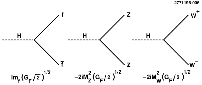
Figure 30: Couplings of the Higgs to fermions and gauge bosons in the Standard Model.

The highly suppressed coupling of the Higgs to fermions makes it difficult to produce the Higgs. A first thought on how to search for a Higgs might be to produce it in $e^{+}e^{-}$ collisions: $e^{+}e^{-}\to H\to f\bar{f}$ and look for the resonance peak. However, the cross section for that process is tiny:

$$\sigma(s=M_{H}^{2}) \sim 0.0005{\rm nb}$$ (46)

for a 10 GeV Higgs and this is to be compared with the cross section for producing quarks at the energy which is 3.65 nb. The resonance bump would not be experimentally observable.

A much more promising way to search for the Higgs is to take advantage of the large coupling of the Higgs to the gauge bosons in order to produce the Higgs. If the Higgs is heavy enough ($M_{H}\geq 2M_{W}$) one can also use gauge bosons in the final state to search for the Higgs.

Higgs Searches at LEP

There were experiments that gave somewhat model dependent limits on the neutral Higgs mass before LEP, but the LEP searches are the most comprehensive. The way that the LEP experiments search for the Higgs is the bremsstrahlung process illustrated in Figure 31. The search is optimized as a function of the mass of the Higgs and since all the LEP searches are only sensitive to Higgs masses where $M_{H}\leq M_{Z}$, they look for decays to fermions in the final state. The searches all take advantage of the fairly unique topology of the events illustrated in Figure 31: a Higgs decaying to a fermion pair or hadrons recoiling against a $Z$ that decays to leptons or neutrinos. No events have been observed in any of the searches at the $Z$ pole where the LEP I collider was operating at $E_{CM}=92$ GeV leading to a lower limit on the Higgs mass $\!{}^{{\bf?}}$:

$$m_{H} \geq 58.4{\rm GeV/c}^{2}$$ (47)

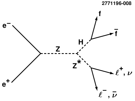
Figure 31: Higgs production in $e^{+}e^{-}$ collisions at the $Z$ pole.

What are our prospects for extending the mass reach in our search for the Higgs? The LEP center of mass energy is currently being extended (LEP II) with the addition of more RF cavities in the machine. Currently LEP is operating at 161 GeV and the ultimate goal is 192 GeV. By looking for $e^{+}e^{-}\to ZH$, a neutral Higgs can be discovered up to a mass of $M_{H}\sim 0.97(E_{CM}-M_{Z})\sim 95$ GeV/c². If the neutral Higgs is not found at LEP II, we will probably need to wait until LHC.

High Mass Higgs Searches at LHC

If we speculate that LEP II does not discover a neutral Higgs and puts a lower limit on its mass of 95 GeV/c², what is next? The next machine on the high energy frontier (as it is often poetically called) is the Large Hadron Collider: LHC. The LHC will collide 7 TeV protons on 7 TeV protons in the LEP tunnel. The design luminosity of the machine is $1\times 10^{34}$ cm^-2s^-1, higher than any storage ring ever built, and searching for the Higgs is one of the design goals of the experiment. There will be two detectors operating at LHC: CMS and ATLAS. The detectors are being optimized to be sensitive to the existence of a Higgs to the full kinematic range of the machine (a mass reach of about 1TeV/c²). Let’s speculate a bit on how to search for the Higgs at LHC, if the Higgs has not been discovered before LHC turns on (around 2005).

The production mechanisms for the Higgs at a proton-proton collider are direct production, gluon-gluon fusion or intermediate boson fusion, as illustrated in Figure 32.

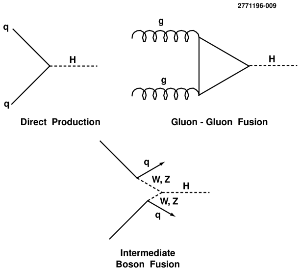
Figure 32: Higgs production in $pp$ collisions at the LHC.

The search strategy for finding the Higgs at LHC depends on the Higgs mass. At high mass ($M_{H}\geq 130$GeV/c²) the search is straightforward. One looks for $pp\to H\to ZZ^{*}~{}{\rm or}~{}ZZ$ with the $Z$’s decaying to leptons. The final state is clean and backgrounds seem manageable. The main issue is luminosity, particularly as one goes to higher mass and the natural width of the Higgs becomes large. One needs 10 fb^-1 of data (one year at 1/10 design luminosity) to discover a 500 GeV/c² Higgs in this channel, and 100 fb^-1 of data (one year at full design luminosity) to discover an 800 GeV/c² Higgs $\!{}^{{\bf?}}$.

The most challenging problem facing LHC experiments is to detect a Higgs in the intermediate mass range: 95 GeV/c${}^{2}\leq M_{H}\leq 130$GeV/c². The dominant decay mode of the Higgs in this mass range will be to two $b$ quarks; a final state for which there will be an enormous QCD background. The rare decay $H\to\gamma\gamma$ is the only hope in this region and even that will be tough. One needs good electromagnetic calorimetry and a lot of data.

I want to stress that it is extremely important that we cover the entire range of possible Higgs mass completely and convincingly. Any hole of 10 or 20 GeV/c² could be fatal since that is where the Higgs might be hiding!

I have discussed the search for Higgs at some length because the existence of the Higgs is, as stated earlier, the most important prediction of the SM that has not been verified. It is also where, if there are to be answers to our questioning of whether the minimal SM is really it, we hope to have the first hints of answers. Most extensions of the SM have a Higgs sector. For example, the minimal supersymmetric SM has two Higgs doublets, with one charged Higgs, two neutral scalars and one pseudoscalar, all waiting to be discovered. However, searching for the Higgs is not the only way to look for new physics.

5.2 Precision Tests of the Standard Model at the $Z$ Pole

The most stringent tests of the SM are the elegant series of analyses being done at LEP and SLC to make precision measurements of SM observables at the $Z$ pole. These experiments offer less hope to discover new physics than Higgs searches, since if discrepancies with the SM turn up, we may have to wait for the higher energy machines to resolve the discrepancies and uncover the new physics that causes them. In a crude sense, precision experiments can tell us if something is wrong with a theory, but they can’t necessarily tell us the cause.

In Section 4.2, I discussed the measurement of the $Z$ mass. However, the LEP experiments can do a great deal more with the approximately 6 million $Z$ decays they have accumulated. They can do precision studies of how the $Z$ decays, and make detailed measurements of the coupling of the $Z$ to the matter fields of quarks and leptons.

For the lepton and $b$ and $c$ quark flavor final states, one can count the number of decays to an exclusive lepton or quark pair which, for each species, is proportional to the squares of the axial and vector coupling of the fermion or quark to the $Z$. One can form forward-backward asymmetries, where one keeps track of the direction of the fermion or quark with respect to the incident electron direction, and at SLC, where the incoming electron beam can be polarized, one can also form right-left asymmetries from the cross section measured with right or left handed incoming electrons. The asymmetries are proportional to the product of the vector and axial coupling of the fermion or quark to the $Z$. At tree level, all the asymmetries and partial widths are completely determined from $G_{F},\alpha_{EM},\alpha_{s}$ and $M_{Z}$, all of which are now well measured. The one loop electroweak radiative corrections depend on $m_{t}$ and $M_{H}$, as well as any possible new physics. What can we do with the wealth of precision measurements available?

The most straightforward thing to do with all the LEP/SLC precision measurements is to input the best experimental values for $G_{F},\alpha_{EM},\alpha_{s},M_{Z}$, $m_{t}$, and some reasonable range of values for $M_{H}$ (such as 60 GeV/c${}^{2}\leq M_{H}\leq 1$TeV/c²) and then see if the predictions of the SM can be verified on a case by case basis with the precision measurements of asymmetries and partial widths. The results of this approach are shown in Figure 33, where I have plotted the ratio of the SM value for the experimental quantities to the SM prediction $\!{}^{{\bf?}}$. The points include LEP data, the $W$ mass measured at FNAL, and the deep inelastic neutrino scattering results. We see in Figure 33 that the SM is doing amazingly well!

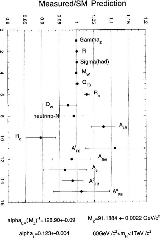
Figure 33: Comparison of experimental measurements with Standard Model predictions for the precision electroweak observables. The input values for the Standard Model parameters are shown.

There is only one result that was causing concern at the time I gave these lectures and that was the measurement of $R_{b}$, the partial width for the $Z$ to decay to $b$ quarks, which was almost four sigma above its predicted value.

We can now think of doing the exercise with the Higgs that we did with the top quark, and use these precision results to “measure” the Higgs mass through the effect that $M_{H}$ exerts on the radiative corrections to these observables. In order to do this, we will have to assume that there is no new physics beyond the SM. The exercise is more difficult than in Section 4.2 where we used the precision measurements to determine the top quark mass. In that case, $\delta r$ depended quadratically on $m_{t}$, but it depends only logarithmically on $M_{H}$. Using the data in Figure 33 one finds $M_{H}\leq 320(430)$ GeV/c² at 90(95)% confidence level but the constraint of a low Higgs mass is driven largely by the measurements of $R_{b}$ and $A_{LR}$ which show, in this data, slight discrepancies with the SM predictions $\!{}^{{\bf?}}$. I personally don’t take the limits on the Higgs mass from this kind of global fit very seriously. I would need to be convinced that the discrepancies in $R_{b}$ and $A_{LR}$ are real before buying stock in a low mass Higgs.

A preferable way to test the SM with the precision electroweak measurements is to try to see if one can limit possible deviations from the SM in some model independent way. There are several schemes that are popular for doing this. Their authors usually consider the general effects on the neutral current and the $Z$ and $W$ pole observables of new heavy physics which contributes to the $Z$ and $W$ self energies but doesn’t have direct coupling to ordinary fermions.

One such scheme that is popular with experimentalists is the $STU$ scheme of Peskin and Takeuchi $\!{}^{{\bf?}}$, where the effects of new physics are parameterized in terms of changes of the boson self energies:

• T is proportional to the difference between the $W$ and $Z$ self energies at $Q^{2}=0$.

• S is the difference between the $Z$ self energy at $Q^{2}=M_{Z}^{2}$ and $Q^{2}=0$.

• S+U is the difference between the $W$ self energy at $Q^{2}=M_{Z}^{2}$ and $Q^{2}=0$.

The interested reader can find this scheme described in more detail in the references $\!{}^{{\bf?}}$. Most of the electroweak observables depend on $S$ and $T$ only, and in the SM, $S=T=U=0$. Figure 34 $\!{}^{{\bf?}}$ shows all the data on the $S-T$ plane and we see that all of the measurements are consistent with no new physics. The contours drawn assume $M_{H}=300$ GeV/c², with the exception of the two contours for all data which are displaced slightly upward (downward) corresponding to $M_{H}=1000(60)$ GeV/c². We see that while the lightest mass allowed for the Higgs is favored, the data are not yet very sensitive to $M_{H}$ and the full range on the Higgs mass from $60$ GeV/$c^{2}$ to 1 TeV/$c^{2}$ is still allowed.

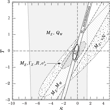
Figure 34: Constraints on extensions of the Standard Model from the precision electroweak data.

5.3 Other Tests of the Standard Model and Searches for New Physics

I have certainly not exhausted all of the tests of the SM that are going on. The two I have discussed so far are the most focused, but there are a slew of other experiments that are looking for processes forbidden in the SM or very highly suppressed, and whose appearance at an unexpectedly high level might be a hint of something new!

Examples of such experiments are:

• the search for flavor changing neutral currents

• searches for lepton number violation

• tests of CPT invariance

• limits on proton decay

and many others. These tests of the SM have proved extremely useful in constraining new physics proposed by theorists. Recently, however, they have not produced any surprises. Nevertheless, it is important to keep looking.

5.4 The Status of the Standard Model

As we have seen, the SM has proved very robust, and it has proved frustratingly successful in predicting experimental results. When I gave these lectures at TASI in June of 1996, I was able to point to a few experimental results that were slightly out of line with theoretical predictions. Keeping in mind the warning that, to date, every experiment has either confirmed the SM predictions or the experiment has been wrong, I discussed the “rogue” results. By the end of the summer, however, all of the discrepancies we were seeing in June had gone away.

R_b

As can be seen in Figure 33, the measured value of $R_{b}$, the fraction of time the $Z$ decays to a pair of $b$ quarks, was almost four standard deviations above its predicted value. The value used in the figure comes from taking the results published by the four LEP experiments and averaging them $\!{}^{{\bf?}}$. However, at the 1996 summer conferences, two new measurements of $R_{b}$ were announced by the ALEPH and SLC collaborations $\!{}^{{\bf?}}$ which were both more in line with the SM expectation, and the problem seems to be going away.

Quark Substructure

Last year the CDF collaboration published a result that could be interpreted as evidence for quark substructure $\!{}^{{\bf?}}$. They saw an excess of jets at high transverse energy in their jet differential cross section distribution when compared with the expectations of next to leading order QCD. However, the other detector operating at the Tevatron, D0, did not see a similar excess, and the theoretical errors associated with the parton distribution functions are probably larger than originally thought, and so this problem also seems to be going away $\!{}^{{\bf?}}$.

ALEPH Four Jet Excess

Another interesting result reported in 1996 that was hard to explain within the context of the SM was an excess of four jet events reported by the ALEPH collaboration from a supersymmetry search looking for $e^{+}e^{-}\to hA$ in their high energy (130-136 GeV center of mass) data $\!{}^{{\bf?}}$. They found an excess of events (16 events on a background of 8.6) at a dijet mass of 105 GeV/c². However, none of the other LEP experiments could reproduce the result and the peak in the ALEPH data appears to have been a statistical fluctuation $\!{}^{{\bf?}}$.

Neutrino Oscillations

An experiment that is worth keeping an eye on is the recent report of evidence for neutrino oscillations from Los Alamos $\!{}^{{\bf?}}$. The SM has no problem with a neutrino mass (in fact it seems unnatural for the neutrino to be exactly massless). If neutrinos do have a mass then it is expected that the lepton numbers won’t be separately conserved and there will be lepton mixing analogous to the quark flavor mixing already observed.

The Los Alamos experiment takes a beam of $\bar{\nu}_{\mu}$ produced by positive muons that are made by protons on a water target making pions and kaons which are then charge selected. The positive muons decay via $\mu^{+}\to e^{+}\nu_{e}\bar{\nu}_{\mu}$. The experiment searches for $\bar{\nu}_{e}$ downstream of the $\bar{\nu}_{\mu}$ beam (the result of a $\bar{\nu}_{\mu}$ to $\bar{\nu}_{e}$ oscillation) via the reaction $\bar{\nu}_{e}+p\to e^{+}+n$. They see 22 $\bar{\nu}_{e}$ events with an expected background of $4.6\pm 0.6$ events. If confirmed, this fills out the SM in a rather attractive way, but any future explanation for quark mixing will have to explain lepton mixing as well.

5.5 The Future

I want to end with a peek into the future. What will our reach be in terms of probing the SM in the next decades? Where will the action be? What will we hope to learn?

The Near Term Future

In the very near term we will be hearing from FNAL and LEP II. LEP II is pushing to the highest energy $e^{+}e^{-}$ center of mass energy ever achieved. They are currently running at 161 GeV and have an eventual goal of about 195 GeV. They will put the best limits on the SM Higgs mass until well into the next decade.

FNAL will be upgrading its luminosity by a factor of 10 by the end of the decade. This will allow them to have a much larger top sample and they will be the only machine looking at top until well into the next decade. FNAL will also have the highest energy reach of any machine, and the upgrade deepens that reach as the increased luminosity helps populate the high energy tails of the parton energy distributions. They will have the best chance of discovering supersymmetric particles such as squarks and gluinos.

The other area of intense experimental activity in the next decade is at the B-factories. These are $e^{+}e^{-}$ machines operating at a center of mass energy of 10.58 GeV that will explore CP violation in $B$ mesons and hopefully nail down the parameters of quark mixing.

On the Horizon: The LHC

The next big machine will be the Large Hadron Collider: LHC. This is a proton-proton collider that will run at CERN starting around 2005. The machine and detectors are being designed to have sensitivity to the largest possible Higgs mass range, since probing the origins of mass at the electroweak scale is a major focus of interest. They will also be able to probe supersymmetry since gluinos and squarks will be copiously produced (if they exist). With a mass reach of about 1.5 TeV in the supersymmetric particle searches, it is very likely that LHC will be able to confirm or exclude the existence of supersymmetry. The LHC has been approved and is under construction. There are two big detector collaborations formed (CMS and ATLAS) and detector designs are well along.

Over the Horizon: What is Next After LHC?

A serious question confronting the experimental community is: what is next? What is the next machine after the LHC that we will want to build? I don’t know the answer to that question. I will present some of the ideas and proposals being discussed. I want to alert you to this debate because the outcome will profoundly affect your future! This is the beginning of the process that will decide what data will be coming in during your career lifetime. The LHC and this next machine will dominate the first 20 or more years of the next century. It is a crucial decision.

The most serious option for a next machine after the LHC is an $e^{+}e^{-}$ linear collider $\!{}^{{\bf?}}$. This is a machine that would start with a center of mass energy of 500 GeV and might eventually be upgraded to 1.5 TeV. If the minimal supersymmetric Standard Model is right, this machine could be a gold mine since most of the Higgses and superpartners would be accessible even at 500 GeV center of mass energy. While the discovery of SUSY might still take place at LHC, the $e^{+}e^{-}$ linear collider offers a much cleaner experimental environment to fully study the SUSY particle spectrum. If, however, the minimal supersymmetric model is wrong, then this machine needs to push to the highest center of mass energies of over 1 TeV in order to extend our physics reach past what already will be learned from the LHC.

Another option that is being discussed as a future machine is an even higher energy proton-proton collider, with 100 TeV of energy in the center of mass. This would be a frontier machine that would push to the highest possible energy just to see what is there $\!{}^{{\bf?}}$.

A final option being discussed is a $\mu^{+}\mu^{-}$ collider. One wins with muons over electrons since electron colliders are limited by radiation which is much suppressed for muons because of their larger mass. The talk is of a muon collider with 4 TeV in the center of mass. $\!{}^{{\bf?}}$

At this point, I don’t know what direction the field will go and I don’t know when a decision will be made about what machine will be built after the LHC. My message that I want to leave the reader with is that you should care which of these machines is built because the choice will determine the experimental results that will be available during your career.

I would also like to remind the reader that it is important to keep an open mind. I suspect that we know less about the way the world works than we think we do. I don’t know if the critical data is already in our hands, whether it will come from a high energy machine, or whether it will come from an unexpected direction such as proton decay, neutrino oscillations, or high energy cosmic rays, but I do believe that we are still in for some surprises!

References

References

- [1] M.Kobayashi and T. Maskawa, Prog. Theor. Phys. 49, 652 (1973).
- [2] S. Weinberg, Phys. Rev. Lett. 19, 1264 (1967).
- [3] S. Glashow, NPB 22, 579 (1061); A. Salam Nobel Symposium, 367, 1968.
- [4] G. t’Hooft, NPB 33, 173 (1971);G. t’Hooft, NPB 35, 167 (1971).
- [5] Chris Quigg, Gauge Theories of the Strong, Weak, and Electromagnetic Interactions, The Benjamin/Cummings Publishing Company, Menlo Park, CA, 1983.
- [6] F. J. Hasert et al., PLB 46, 138 (1973).
- [7] A. Blondel et al., ZPC 45, 361 (1990).
- [8] L. L. Lewis et al., PRL 39, 795 (1977); P. E. G. Baird et al., PRL 39, 798 (1977).
- [9] P. Bucksbaum, E. Commins, and L. Hunter, PRL 46, 540 (1981); P. Bucksbaum, E. Commins, and L. Hunter, PRD 24, 1134 (1981); P. S. Drell and E. D. Commins, PRL 53, 968 (1984); P. S. Drell and E. D. Commins, PRA 32, 2196 (1985).
- [10] C. Prescott et al., PLB 77, 347 (1978); C. Prescott et al., PLB 84, 524 (1979)
- [11] Konrad Kleinknecht, Detectors for Particle Radiation, Cambridge University Press, Cambridge,1987.
- [12] Particle Data Group, PRD 54, (1996)
- [13] Tran N. Truong, PRD 30, 1509 (1984); F. J. Gilman and S. H. Rhie, PRD 31, 1066 (1985).
- [14] Persis S. Drell and J. Ritchie Patterson, “Weak Decays, Rare Decays, Mixing and CP Violation” In Proceedings of the XXVI International Conference on High Energy Physics, Dallas, 1992 edited by J. R. Sanford,(AIP, 1993).
- [15] V. E. Barnes et al., PRL 12, 204 (1964).
- [16] R. Barbieri et al., PLB 95, 93 (1980); B. P. Mackenzie and G. P. Lepage, PRL 47, 1244 (1981).
- [17] E. A. Kuraev and V. S. Fadin, Sov. J. Nucl. Phys 41, 466 (1985); F. A. Berends, G. J. H. Burgers and W. L. Van Neerven, PLB 185, 395 (1987).
- [18] J. Erler and P. Langacker, PRD 52, 441 (1995).
- [19] M. L. Swartz, “Tests of the Electroweak Standard Model at High Energies ( GeV)”, In Proceedings of the XVI International Lepton Photon Conference, Ithaca, 1993 edited by Persis Drell and David Rubin, (AIP, 1994).
- [20] C. Athanassopoulos et al., “Evidence for Oscillations from the LSND Experiment at LAMPF”, LA-UR-96-1582.
- [21] C. Campagnari and M. Franklin, “The Discovery of the Top Quark”, UCSB-HEP-96-01, HUTP-96/A023.
- [22] F. Abe et al. PRL 74, 2662 (1995).
- [23] N. Isgur and M. Wise, PLB 232, 113 (1989); N. Isgur and M. Wise, PLB 237, 527 (1990)
- [24] B. Barish et al. PRD 51, 1014 (1995).
- [25] M. E. Peskin and D. V. Schroeder, An Introduction to Quantum Field Theory, Addison-Wesley Publishing Company, Menlo Park, CA, 1995.
- [26] I. Hinchliffe and J. Womersley, “High Transverse Momentum Physics at the Large Hadron Collider”, LBNL-38997.
- [27] M. Peskin and T. Takeuchi, PRL 65, 964 (1990) and PRD 46, 381 (1992).
- [28] The ALEPH Collaboration, “A Measurement of using Mutually Exclusive Tags”, Contribution to the XXVII International Conference on High Energy Physics, ICHEP, Warsaw, Poland, 25-31 July, 1996, The SLD Collaboration, “Measurement of at SLD”, SLAC-PUB-96-7170.
- [29] F. Abe et al. PRL 77, 438 (1996)
- [30] S Abachi et al., “Inclusive Jet Cross Section at D0”, FERMILAB-CONF-96/280-E.
- [31] D. Buskulic et al., “Four-jet final state production in collisions at centre-of-mass energies of 130 and 136 GeV”, CERN PPE/96-052.
- [32] The DELPHI Collaboration, “Search for Pair Production of Heavy Objects in 4-jet Events with the DELPHI Detector at GeV”, Contribution to the XXVII International Conference on High Energy Physics, ICHEP, Warsaw, Poland, 25-31 July, 1996.
- [33] The NLC Design Group, “Zeroth-Order Design Report for the Next Linear Collider”, SLAC-474.
- [34] Gerry Dugan, “Really Large Hadron Colliders”, Cornell Preprint CBN96-12.
- [35] A. N. Skrinsky and V. V. Parkhomchuk, Sov. J. Nucl. Physics, 12, 3 (1981); D. Neuffer, Part. Accel., 14, 75 (1983).