Accurate Measurement of $F_{2}^{\rm d}/F_{2}^{\rm p}$ and $R^{\rm d}-R^{\rm p}$

Abstract

Results are presented for $F_{2}^{\rm d}/F_{2}^{\rm p}$ and $R^{\rm d}-R^{\rm p}$ from simultaneous measurements of deep inelastic muon scattering on hydrogen and deuterium targets, at 90, 120, 200 and 280 GeV. The difference $R^{\rm d}-R^{\rm p}$, determined in the range $0.002<x<0.4$ at an average $Q^{2}$ of 5 GeV², is compatible with zero. The $x$ and $Q^{2}$ dependence of $F_{2}^{\rm d}/F_{2}^{\rm p}$ was measured in the kinematic range $0.001<x<0.8$ and $0.1<Q^{2}<145$ GeV² with small statistical and systematic errors. For $x>0.1$ the ratio decreases with $Q^{2}$.

(to be submitted to Nuclear Physics)

———————————–

For footnotes see next page.

+	Supported by Bundesministerium für Bildung und Forschung.
++	Supported in part by FOM, Vrije Universiteit Amsterdam and NWO.
*	Supported by KBN SPUB Nr 621/E - 78/SPUB/P3/209/94.
**	Laboratory of CEA, Direction des Sciences de la Matière.
a)	Now at CERN, 1211 Genève 23, Switzerland.
b)	Now at NIKHEF, 1009 DB Amsterdam, The Netherlands.
c)	Now at University of Padova, 35131 Padova, Italy.
d)	Now at MPI für Kernphysik, 69029 Heidelberg, Germany.
e)	Now at Université de Genève, 1211 Genève 4, Switzerland.
f)	Now at DPTA, CEA, Bruyères-le-Chatel, France.
g)	Now at Yale University, New Haven, 06511 CT, U.S.A.
h)	Now at University of Mainz, 55099 Mainz, Germany.
i)	Now at University of Bonn, 53115 Bonn, Germany.
j)	Now at INFN-Istituto Superiore di Sanità, 00161 Roma, Italy.
k)	Now at Osaka University, 567 Osaka, Japan.
l)	Now at University of Michigan, Michigan, U.S.A.
m)	Now at Stockholm University, 113 85 Stockholm, Sweden.
n)	Now at University of Erlangen-Nürnberg, 91058 Erlangen, Germany.
o)	Now at IKP2-KFA, 52428 Jülich, Germany.
p)	Now at University of Houston, 77204 TX, U.S.A.
q)	Now at Dresden University, 01062 Dresden, Germany.
r)	Now at ESRF, 38043 Grenoble, France.
s)	Now at Tokyo Institute of Technology, Tokyo, Japan.
t)	Now at University of Freiburg, 79104 Freiburg, Germany.
u)	Now at Warsaw University of Technology, Warsaw, Poland.
v)	Now at University of Hamburg, 22761 Hamburg, Germany.

1 Introduction

In this paper we present an accurate, high statistics measurement of the ratio of the structure functions of the deuteron and the proton, $F_{2}^{\rm d}/F_{2}^{\rm p}$, and of the difference, $R^{\rm d}-R^{\rm p}$, obtained in deep inelastic muon scattering at incident energies of 90, 120, 200 and 280 GeV. Here, $R$ is the ratio of longitudinally to transversely polarised virtual photon absorption cross sections. The main motivations for this measurement are as follows:

• From the measured ratio $F_{2}^{\rm d}/F_{2}^{\rm p}$, the ratio of the neutron and proton structure functions can be extracted. In the parton picture of the nucleon $F_{2}^{\rm n}/F_{2}^{\rm p}$ is related to the ratio of the down and up quark momentum distributions. Thus, a precise measurement of $F_{2}^{\rm d}/F_{2}^{\rm p}$ puts strong constraints on the flavour composition of the nucleon as a function of the quark momentum.

• Although the proton and neutron have different flavour compositions, the $Q^{2}$ dependences of $F_{2}^{\rm p}$ and $F_{2}^{\rm d}$ are similar, resulting in a slight $Q^{2}$ dependence of $F_{2}^{\rm d}/F_{2}^{\rm p}$ which can be calculated in perturbative QCD.

• Perturbative QCD also predicts that $\Delta R=R^{\rm d}-R^{\rm p}$ is sensitive to differences in the gluon distributions of the proton and the neutron. Thus, through a measurement of $\Delta R$ one can estimate such differences.

The differential cross section for one photon exchange can be written in terms of the nucleon structure function $F_{2}(x,Q^{2})$ and the ratio $R(x,Q^{2})$ as

$$\frac{{\rm d}^{2}\sigma(x,Q^{2},E)}{{\rm d}x{\rm d}Q^{2}} = \frac{4\pi\alpha^{2}}{Q^{4}}\cdot\frac{F_{2}(x,Q^{2})}{x}\cdot$$ (1)

$$\left\{1-y-\frac{Q^{2}}{4E^{2}}+(1-\frac{2m^{2}}{Q^{2}})\cdot\frac{y^{2}+Q^{2}/E^{2}}{2\left(1+R(x,Q^{2})\right)}\right\}\,\,,$$

where $\alpha$ is the fine structure constant, $-Q^{2}$ the four-momentum transfer squared, $E$ the energy of the incident muon and $m$ the muon mass. The Bjorken scaling variable, $x$, and $y$ are defined as $x=Q^{2}/2M\nu$ and $y=\nu/E$, where $\nu$ is the energy of the virtual photon in the target rest frame and $M$ the proton mass. Throughout this paper, cross sections and structure functions are always given per nucleon.

To extract the structure function ratio, $F_{2}^{\rm d}/F_{2}^{\rm p}$, and the difference, $R^{\rm d}-R^{\rm p}$, from the cross section ratio, $\sigma_{\rm d}/\sigma_{\rm p}$, measurements at different incident energies with a large overlap in $x$ and $Q^{2}$ are needed. If $R^{\rm d}=R^{\rm p}$, the ratios $\sigma_{\rm d}/\sigma_{\rm p}$ and $F_{2}^{\rm d}/F_{2}^{\rm p}$ are equal, as is apparent from eq.(1).

In the present experiment the ratio $\sigma_{\rm d}/\sigma_{\rm p}$ was obtained from a simultaneous measurement on hydrogen and deuterium in a symmetric target arrangement. This results in a cancellation of systematic errors due to spectrometer acceptance and normalisation and allows measurements in kinematic regions where the detector acceptance is small.

The results presented here use the full NMC proton and deuteron data; they supersede those already published in refs. [1, 2, 3] that were based on part of the data. They cover a broad kinematic range $0.001<x<0.8$ and $0.1<Q^{2}<145$ GeV² and have total systematic errors typically below 1%.

2 The experiment

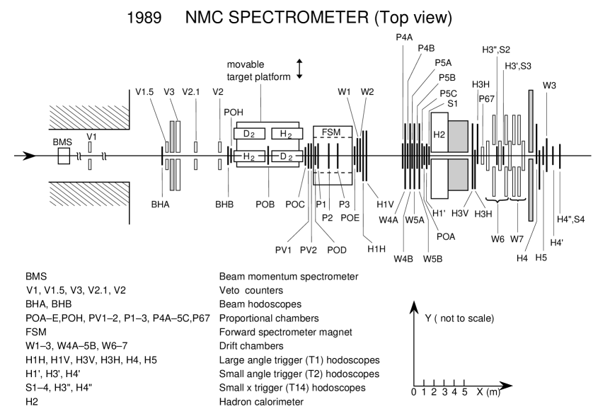
Figure 1: The NMC spectrometer for the 1989 data taking. The beam calibration spectrometer is located downstream and not shown.

The NA37 experiment was performed at the M2 muon beam line of the CERN SPS. The data were taken in 1986 and 1987 at nominal incident energies of 90 and 280 GeV, and in 1989 at 120, 200 and 280 GeV. The spectrometer is described in detail in refs. [2, 4] and the layout for the 1989 run is shown in fig. 1.

The momenta of the incoming muons were determined with a beam momentum spectrometer (BMS) and their positions in two hodoscopes (BHA, BHB) upstream of the targets. Scattered muons and produced hadrons were measured in a forward spectrometer consisting of a dipole magnet (FSM), proportional chambers (P), drift chambers (W) and trigger hodoscopes (H, S). Particles passing through a 2 m thick iron absorber were identified as muons.

The measurements were performed simultaneously on hydrogen and deuterium. The target system contained two sets of target pairs which were alternately exposed to the beam. In one pair the upstream target was liquid hydrogen and the downstream one liquid deuterium, while in the other pair the order was reversed. Frequent exchange of the two target sets (typically twice per hour) minimised the effect of any time dependent detector response. The targets were contained in 3 m long mylar cells. Their thicknesses were 21.06(1) g/cm² for H₂ and 48.58(1) g/cm² for D₂ with a 3.0(2)% HD admixture in the D₂. The total amount of mylar in the beam was 0.12 g/cm² per target, including target superinsulation.

For the 1989 data taking, upgrades were made to extend the accessible kinematic range towards smaller scattering angles, $\theta$, thus allowing smaller values of $x$ to be reached. The longitudinal vertex resolution was improved by adding an extra tracking chamber with 1 mm wire spacing (P0H) in front of the upstream target. To detect muons scattered at small angles, an additional trigger system (T14) was set up in addition to the two triggers (T1,T2) described in ref. [2], by using small scintillators (S1, S2, S4) placed just above and below the muon beam [5]. In this trigger only the central part of the beam was used to avoid triggering on divergent beam tracks. Additional tracking chambers (P67, W3) were installed behind the iron absorber to improve the reconstruction of small angle tracks. Also, the performance of the small angle trigger (T2) was improved considerably so that a large increase in the yield at small $x$ values was obtained in 1989.

The calibration of the scattered and incident muon momenta was done using various methods. The forward spectrometer magnet was calibrated to an accuracy of 0.2% by comparing the observed J/$\psi$ and K⁰ masses with their known values. The beam momentum spectrometer was calibrated in dedicated runs by remeasuring the incident muon momentum in a purpose built spectrometer [6]. An independent calibration of the BMS relative to the FSM was obtained using silicon microstrip detectors [7]. The two BMS calibrations were averaged, leading to an accuracy in the incident muon momentum of 0.2%.

3 Data analysis

3.1 Extraction of $\sigma_{\rm d}/\sigma_{\rm p}$

The ratio of cross sections for the deuteron and the proton was obtained from the measured numbers of events in the four targets. The description of the event reconstruction can be found in refs. [2, 4, 5]. In any ($x$,$Q^{2}$) bin the number of scattered muons detected in the spectrometer and originating e.g. in the upstream hydrogen target is given by

$$N_{\rm p}^{\rm up}=\phi_{1}\rho_{\rm p}\sigma_{\rm p}^{\rm incl}A_{\rm p}^{\rm up}.$$ (2)

Here $\phi_{1}$ is the integrated beam flux illuminating the targets of the first set, $\rho_{\rm p}$ the number of target nucleons per unit area, $\sigma_{\rm p}^{\rm incl}$ the inclusive cross section per nucleon and $A_{\rm p}^{\rm up}$ the acceptance. With equivalent expressions for the other three targets one obtains

$$\frac{\sigma_{\rm d}^{\rm incl}}{\sigma_{\rm p}^{\rm incl}}=\frac{\rho_{\rm p}}{\rho_{\rm d}}\sqrt{\frac{N_{\rm d}^{\rm up}N_{\rm d}^{\rm down}}{N_{\rm p}^{\rm up}N_{\rm p}^{\rm down}}}\,\,,$$ (3)

under the assumption that $A_{\rm d}^{\rm up}=A_{\rm p}^{\rm up}$ and $A_{\rm d}^{\rm down}=A_{\rm p}^{\rm down}$. Thus the measured cross section ratio does not depend on the incident muon flux or the detector acceptance.

To obtain the ratio of one photon exchange cross sections, $\sigma_{\rm d}/\sigma_{\rm p}$, the numbers of events in eq.(3) were replaced by the accumulated weights, $\sigma/\sigma^{\rm incl}$, to correct for higher order electroweak processes. These radiative corrections were calculated using the method of ref. [8] as described in ref. [9]. This procedure includes corrections for the radiative tails of elastic and quasi-elastic scattering as well as for the inelastic radiative tails. For the calculation of the latter the structure function $F_{2}$ and the ratio $R$ are needed. Therefore the extraction of $\sigma_{\rm d}/\sigma_{\rm p}$ was performed in an iterative procedure. The structure function $F_{2}^{\rm p}$ was fixed to the parametrisation of NMC, SLAC and BCDMS data from ref. [10] and for $R$ the parametrisation of ref. [11] was used. The structure function $F_{2}^{\rm d}$ was taken as the product of $F_{2}^{\rm p}$ and $\sigma_{\rm d}/\sigma_{\rm p}$, which was determined from a fit in $x$ and $Q^{2}$ to the presently measured ratio, assuming $R^{\rm d}=R^{\rm p}$. For the extrapolation of $F_{2}^{\rm p}$ to $Q^{2}=0$, the model of Donnachie and Landshoff [12] was used, while $R$ was assumed to be constant below $Q^{2}=0.35$ GeV². For the form factor of the nucleon the parametrisation of Gari and Krümpelmann [13] was used and for the deuteron the parametrisation of  Švarc and Locher [14]. The suppression of quasi-elastic scattering in the deuteron was evaluated using the results of a calculation of Bernabeu and Pascual [15]. The iteration was stopped when the change in $\sigma_{\rm d}/\sigma_{\rm p}$ was less than 0.1% in every $x$ and $Q^{2}$ bin.

To estimate the error due to radiative corrections the prescription given in ref. [2] was followed. For this estimate the upper and lower bounds of $F_{2}^{\rm p}$ from ref. [10] were used and the uncertainty on $R$ for $Q^{2}>0.35$ GeV² was taken to be that of the parametrisation of ref. [11] enlarged by 50%; for $Q^{2}$ below 0.35 GeV² an error on $R$ of +150% and –100% was assumed. For the form factors and the suppression factor alternative parametrisations were used to estimate the associated systematic uncertainties. To estimate the influence of the functional form chosen to parametrise $\sigma_{\rm d}/\sigma_{\rm p}$, the procedure was repeated with a parametrisation of $\sigma_{\rm d}/\sigma_{\rm p}$ that was a function of $x$ only. The total error due to the radiative corrections was at most 2% at the smallest $x$.

3.2 Data selection

To check the assumption of equal acceptances for the two upstream and the two downstream targets the beam flux ratio

$$\frac{\phi_{2}}{\phi_{1}}=\sqrt{\frac{N_{\rm d}^{\rm up}N_{\rm p}^{\rm down}}{N_{\rm p}^{\rm up}N_{\rm d}^{\rm down}}}$$ (4)

was used. It should not depend on any variable characterising the event. Thus, cuts were applied in order to remove events from kinematic regions where the flux ratio was not constant, e.g. at the edges of the distributions of the scattering angle, $\theta$, and the energy transfer, $\nu$.

The time dependence of the detector acceptance was investigated using the acceptance ratio calculated from

$$\frac{A^{\rm up}}{A^{\rm down}}=\sqrt{\frac{N_{\rm d}^{\rm up}N_{\rm p}^{\rm up}}{N_{\rm d}^{\rm down}N_{\rm p}^{\rm down}}}$$ (5)

for consecutive exposures of the two target sets. No significant time dependence of the ratio was observed except for brief periods where experimental problems could be identified, and whose data were discarded.

In this analysis we have included the information from the large drift chambers (W45) as described in ref. [2] contrary to what was done in the $F_{2}$ analysis [9]. Thus the measurement of cross section ratios could be extended to larger scattering angles and hence to larger $Q^{2}$. Cuts were applied to the incoming muon distributions such that the incident flux was identical for the upstream and downstream targets. Cuts on the interaction vertex position were used to associate the events to one of the targets.

For events selected by the small $x$ trigger, T14, a cut of $x_{\rm min}=0.001$ removed the data around $x=m_{\rm e}/m_{\rm p}=0.544\cdot 10^{-3}$, dominated by elastic scattering from atomic electrons [5, 16]. The contamination from these events in the region with $x>0.001$ was estimated from a Monte Carlo simulation to be less than 0.5% for $x<0.002$ and negligible elsewhere.

The final data samples were obtained from the reconstructed events by applying the kinematic cuts listed in table 1. The cuts exclude kinematic regions where higher order electroweak processes dominate, which are contaminated with muons from hadron decays or have poor kinematic or vertex resolution. In addition, certain ($x,Q^{2}$) bins at the edge of the acceptance were removed; in particular, bins were discarded which had only a few events from one of the targets or if their area $\Delta x\Delta Q^{2}$ was reduced by more than half by the kinematic cuts.

$E$	Trigger	$y_{\rm max}$	$p^{\prime}_{\rm min}$	$\nu_{\rm min}$	$\nu_{\rm max}$	$\theta_{\rm min}$	$\theta_{\rm max}$	No. of events
(GeV)			(GeV)	(GeV)	(GeV)	(mrad)	(mrad)	after cuts
280	T1	0.9	40	10	–	10	–	$1.41\cdot 10^{6}$
	T2	0.9	40	15	–	5	17	$1.75\cdot 10^{6}$
	T14	0.9	40	20	–	3.75	14.4	$0.34\cdot 10^{6}$
200	T1	0.9	30	15	–	10	–	$0.71\cdot 10^{6}$
	T2	0.9	30	20	160	6	17	$0.36\cdot 10^{6}$
	T14	0.9	30	20	–	3.75	14.4	$0.25\cdot 10^{6}$
120	T1	0.9	20	7	–	14.3	–	$1.12\cdot 10^{6}$
	T2	0.9	20	10	90	6	17	$0.31\cdot 10^{6}$
	T14	0.9	20	10	–	3.75	14.4	$0.18\cdot 10^{6}$
90	T1	0.9	15	5	–	13	–	$1.80\cdot 10^{6}$
	T2	0.9	15	5	–	3	17	$0.18\cdot 10^{6}$

Table 1: Kinematic cuts applied to the eleven data sets classified by energy and trigger. The scattered muon momentum is indicated by $p^{\prime}$.

The total number of events in the analysis after cuts is $2.7\cdot 10^{6}$ for hydrogen and $5.7\cdot 10^{6}$ for deuterium. This is more than double the number of events in the analysis of ref. [2], with the increase largest at small $x$. About a quarter of the events were used in the determination of $F_{2}^{\rm d}$, $F_{2}^{\rm p}$ and $R$ of ref. [17].

3.3 Further corrections to $\sigma_{\rm d}/\sigma_{\rm p}$ and systematic errors

Several corrections were applied to the data in addition to the radiative corrections discussed earlier. The finite resolution of the spectrometer caused some vertices to be reconstructed outside the targets or even to be associated to the wrong target. To estimate the number of such events, the longitudinal vertex distributions were fitted in several intervals of the scattering angle. These fits were used to determine the optimal vertex cuts and the corrections due to the tails of the distributions. These corrections varied between 0.1% and 1% and the error was taken as half the value with a minimum of 0.1%.

The correction due to the finite kinematic resolution of the spectrometer was taken from a Monte Carlo simulation of the experiment. This correction was usually much below 1% except for $x>0.4$ where it reached several percent for the lowest $Q^{2}$ bins. The error was taken to be 30% of the correction.

In addition, the effects of the HD admixture in the deuterium and of the mylar in the beam were taken into account, yielding changes in the ratio of about 1% and 0.3%, respectively. The errors on the ratio due to the uncertainties on these corrections were less than 0.1%.

The corrections were taken into account separately for each of the eleven sets of data listed in table 1. For the further analysis the ratios were interpolated to the centre of each $x$ bin and the results for each incident energy obtained by taking the geometrical average [18] of the corresponding data sets.

The total systematic error on $\sigma_{\rm d}/\sigma_{\rm p}$ was determined by adding in quadrature the contributions from the uncertainties on the muon momenta, on the radiative, vertex and smearing corrections and on those due to the functional form used to describe the ratio during the iterations. The latter four were assumed to be fully correlated between the data sets. The uncertainties in the hydrogen and deuterium densities and target lengths led to an additional normalisation error which is smaller than 0.1% (relative normalisation uncertainties are discussed in section 5).

4 Results for $R^{\rm d}-R^{\rm p}$

The difference $\Delta R=R^{\rm d}-R^{\rm p}$ was determined following the method described in ref. [3]. From eq.(1) the cross section ratio, $\sigma_{\rm d}/\sigma_{\rm p}$, can be related to the structure function ratio, $F_{2}^{\rm d}/F_{2}^{\rm p}$, and $R^{\rm d}$ and $R^{\rm p}$ through

$$\frac{\sigma_{\rm d}}{\sigma_{\rm p}}(x,Q^{2},E)=\frac{F_{2}^{\rm d}}{F_{2}^{\rm p}}(x,Q^{2})\cdot\frac{1+R^{\rm p}(x,Q^{2})}{1+R^{\rm d}(x,Q^{2})}\cdot\frac{1+\varepsilon\cdot R^{\rm d}(x,Q^{2})}{1+\varepsilon\cdot R^{\rm p}(x,Q^{2})}\ .$$ (6)

The dependence of the cross section ratio on the incident energy $E$ appears only through the polarisation parameter $\varepsilon$

$$\varepsilon=\left(1+\frac{1}{2}(1-\frac{2m^{2}}{Q^{2}})\cdot\frac{y^{2}+\frac{Q^{2}}{E^{2}}}{1-y-\frac{Q^{2}}{4E^{2}}}\right)^{-1}.$$ (7)

This coefficient is always smaller than unity and mainly dependent on $y=\nu/E$. Expanding eq.(6) one obtains to first order in $\Delta R$

$$\frac{\sigma_{\rm d}}{\sigma_{\rm p}}\simeq\frac{F_{2}^{\rm d}}{F_{2}^{\rm p}}\left(1-\frac{1-\varepsilon}{(1+\overline{R})(1+\varepsilon\overline{R})}\Delta R\right),$$ (8)

where $\overline{R}=(R^{\rm d}+R^{\rm p})/2$. Because $\Delta R$ is small, $\sigma_{\rm d}/\sigma_{\rm p}$ is insensitive to $\overline{R}$. The sensitivity to $\Delta R$ is largest for those ($x,Q^{2}$) bins where the range in $\varepsilon$ is widest. Fig. 2 shows schematically the behaviour of the cross section ratio as a function of $Q^{2}$ for different energies: the small $Q^{2}$ (large $\varepsilon$) data at each energy are insensitive to $\Delta R$, but at large $Q^{2}$ (small $\varepsilon$) the sensitivity becomes significant. Thus the data at large $\varepsilon$ are mainly sensitive to $F_{2}^{\rm d}/F_{2}^{\rm p}$ while $\Delta R$ is determined by the small $\varepsilon$ data.

We chose to determine a $Q^{2}$-averaged value of $\Delta R$ for each $x$ bin separately, fitting a parametrisation of $\sigma_{\rm d}/\sigma_{\rm p}$ to the data using eq.(6). Four parameters were used: $\Delta R$, $\overline{R}$ and the two parameters of the function $F_{2}^{\rm d}/F_{2}^{\rm p}=a_{1}+a_{2}\ln Q^{2}$. Previous measurements of $R$ [17, 19, 20] were included in the fits to loosely constrain the value of $\overline{R}$. By fitting eq.(6) to all data in each $x$ bin, the $Q^{2}$-averaged value of $\Delta R$ was determined with higher accuracy than would have been achieved if the analysis had been restricted to the regions of overlap in $Q^{2}$. The lowest $x$ bin was excluded because the range in $\varepsilon$ is too small. Data at large $x$ were not included because of their low sensitivity to $\Delta R$. The fits describe the data well in all $x$ bins with a total $\chi^{2}$ of 472 for 515 degrees of freedom.

The systematic errors on $\Delta R$ were calculated by shifting the measured cross section ratios by the error due to each source separately and repeating the fits. All contributions to the error on $\Delta R$ were then added in quadrature. The dominant contributions were due to the uncertainties on the radiative corrections at small $x$, on the normalisation at medium $x$ and on the muon momenta at large $x$.

The results for $\Delta R$ are shown in fig. 3 and listed in table 2; they cover the range $0.003<x<0.35$. The $\langle Q^{2}\rangle$ given in table 2 were evaluated using weights derived from the sensitivity of each of the data points to $\Delta R$. The values of $\Delta R$ are small; this is most significant at small $x$, i.e. small $Q^{2}$, where $R$ is large ($R\approx 0.3$ for $x\approx 0.01$, $Q^{2}\approx 2$ GeV² [17, 19]). No significant $x$ dependence of $\Delta R$ is observed. Averaging the measurements over $x$ one obtains

$$\Delta R=0.004\,\pm\,0.012(\rm{stat})\,\pm\,0.011(\rm{syst.}),$$ (9)

compatible with zero, at $\langle Q^{2}\rangle=$ 5 GeV².

$x$	$\langle Q^{2}\rangle$		$y$ Range		$\varepsilon$ Range		$R^{\rm d}-R^{\rm p}$		Stat.	Syst.
	(GeV2)								error	error
0.0030	0.	68	0.31 –	0.76	0.944 –	0.461		0.045	0.088	0.047
0.0050	0.	99	0.20 –	0.72	0.989 –	0.523		0.103	0.073	0.044
0.0080	1.	8	0.13 –	0.80	0.992 –	0.389		0.002	0.037	0.024
0.0125	2.	9	0.08 –	0.78	0.997 –	0.420	–	0.046	0.038	0.014
0.0175	4.	0	0.09 –	0.79	0.996 –	0.389	–	0.022	0.039	0.011
0.025	5.	0	0.07 –	0.74	0.998 –	0.494		0.023	0.030	0.009
0.035	8.	1	0.06 –	0.77	0.998 –	0.444		0.029	0.038	0.009
0.050	11.	1	0.06 –	0.74	0.998 –	0.492		0.025	0.033	0.007
0.070	15.	3	0.06 –	0.73	0.998 –	0.509	–	0.082	0.046	0.007
0.090	20.	1	0.06 –	0.75	0.998 –	0.468	–	0.025	0.056	0.007
0.110	25.	0	0.06 –	0.77	0.998 –	0.431		0.100	0.062	0.008
0.140	27.	8	0.06 –	0.73	0.998 –	0.506		0.032	0.067	0.012
0.180	37.	1	0.06 –	0.69	0.998 –	0.558	–	0.124	0.084	0.014
0.225	38.	8	0.06 –	0.73	0.998 –	0.507		0.043	0.115	0.022
0.275	57.	2	0.05 –	0.64	0.998 –	0.642		0.082	0.125	0.022
0.350	62.	7	0.04 –	0.60	0.999 –	0.693	–	0.003	0.159	0.039

Table 2: Values of $\Delta R=R^{\rm d}-R^{\rm p}$ determined at $x$ and $\langle Q^{2}\rangle$. The calculation of $\langle Q^{2}\rangle$ takes into account the sensitivity of the data points to $\Delta R$. In addition the $y$ and $\varepsilon$ range of the data for each $x$ bin are given.

In fig. 3 we also show the results on $\Delta R$ at higher $x$ obtained from the SLAC experiment E140X [23] and from a reanalysis of earlier SLAC data [11], which agree very well with the present values. The SLAC results were determined using only kinematic regions where measurements at different energies overlap in $x$ and $Q^{2}$. We have re-evaluated $\Delta R$ from the SLAC data in ref. [11] with the method described above and find almost identical results but with smaller errors [24]. Differences of $R$ have also been measured for several combinations of nuclei (see refs. [3, 21, 22, 23]) and were found to be compatible with zero.

In next to leading order perturbative QCD, the $x$ and $Q^{2}$ dependence of $R$ is related [25] to that of the singlet structure function $F_{2}^{\rm{SI}}$ and the gluon distribution $xG$ through the longitudinal structure function

$$F_{\rm L}(x,Q^{2})=\frac{\alpha_{s}(Q^{2})x^{2}}{2\pi}\int\limits_{x}^{1}\left(\frac{8}{3}F_{2}^{\rm{SI}}(w,Q^{2})+\frac{40}{9}wG(w,Q^{2})(1-\frac{x}{w})\right)\frac{\mbox{d}w}{w^{3}}$$ (10)

and

$$R(x,Q^{2})=\frac{F_{\rm L}(x,Q^{2})+\frac{4M^{2}x^{2}}{Q^{2}}F_{2}(x,Q^{2})}{F_{2}(x,Q^{2})-F_{\rm L}(x,Q^{2})}.$$ (11)

For $x<0.10$, the gluon distribution dominates the integral of eq.(10). Thus, at small $x$, $\Delta R$ is sensitive to the difference between the deuteron and proton gluon distributions. The solid line in fig. 4 shows a QCD prediction for $\Delta R$ assuming equal gluon distributions; the values of $F_{2}$ were taken from ref. [10] and the approximation was made that $F_{2}^{\rm{SI}}\approx F_{2}^{\rm d}$, whereas $xG$ was taken from the QCD analysis in ref. [26]. The dashed and dotted lines in fig. 4 were calculated using a gluon distribution for the deuteron scaled by 1.1 and 1.2, respectively. Within perturbative QCD this sets a limit on a possible difference between the proton and the deuteron gluon distributions of about 10%. We have not investigated the sensitivity of $\Delta R$ to possible higher twist effects.

5 Internal consistency of the data

We have looked for possible normalisation shifts of the data at 90, 120, 200 and 280 GeV by repeating the calculation of $\Delta R$ with four additional normalisation parameters in the fit. The $\chi^{2}$ improvement is not significant and the normalisation shifts suggested by the fit were -0.11%, -0.01%, +0.18% and +0.06%, respectively, with typical errors of 0.16%. This shows that the internal consistency of the data taken over the course of four years is very good. The compatibility of these shifts with zero indicates that there is no additional normalisation uncertainty on $\sigma_{\rm d}/\sigma_{\rm p}$ at the level of 0.15%. The change in $\Delta R$ was everywhere much smaller than the statistical error.

6 Results for $F_{2}^{\rm d}/F_{2}^{\rm p}$

Structure function ratios can be determined from the measured cross section ratios once $\Delta R$ and $\overline{R}$ are known. As $\Delta R$ is compatible with zero we have taken the structure function ratio, $F_{2}^{\rm d}/F_{2}^{\rm p}$, to be equal to the cross section ratio, $\sigma_{\rm d}/\sigma_{\rm p}$.

The geometrical average of the data at the four energies was taken, and the resulting values for $F_{2}^{\rm d}/F_{2}^{\rm p}$ in bins of $x$ and $Q^{2}$ are given in table 3. Fig. 5 shows the ratio as a function of $Q^{2}$ in each $x$ bin. The average systematic error is about 0.4% and almost all the data have a systematic error smaller than 1%. A comparison to results from SLAC [29] and BCDMS [30] for $F_{2}^{\rm d}/F_{2}^{\rm p}$ is shown in fig. 6 for three $x$ bins and demonstrates good agreement.

In most of the $x$ bins the present data cover nearly two decades in $Q^{2}$, with little dependence on $Q^{2}$. To investigate possible $Q^{2}$ dependences, the data were fitted in each $x$ bin with a linear function of $\ln Q^{2}$

$$F_{2}^{\rm d}/F_{2}^{\rm p}=b_{1}+b_{2}\ln Q^{2}.$$ (12)

Fig. 7 shows the fitted slope parameter $b_{2}$ as a function of $x$. The systematic uncertainties on $b_{2}$ were calculated by shifting the ratio by each of its systematic uncertainties and repeating the fits. The resulting contributions were added in quadrature. The results of the fits are given in table 4. The total $\chi^{2}$ of these fits is 202 for 220 degrees of freedom.

Also shown in fig. 7 are two next to leading order QCD calculations, including target mass corrections, based on analyses of the NMC structure function data [27] and of the SLAC and BCDMS data [28]. The measured slopes are consistent with these perturbative QCD calculations although there may be deviations at $x>0.1$ as was suggested in ref. [2]. However, in order to investigate the possible interpretation of the large $x$ data in terms of significant higher twist effects, as was done in ref. [2], a common analysis of the present data and the SLAC and BCDMS results is required.

The results for $F_{2}^{\rm d}/F_{2}^{\rm p}$ averaged over $Q^{2}$ are listed in table 4. The statistical and systematic errors are below 0.5% for most of the $x$ range. The main contributions to the systematic errors stem from the uncertainty of the radiative corrections at small $x$ and the uncertainty in the kinematic resolution and the momentum calibrations at large $x$. The ratio is consistent with unity at the lowest measured $x$.

Neglecting nuclear effects in the deuteron, the neutron structure function is given by $F_{2}^{\rm n}=2F_{2}^{\rm d}-F_{2}^{\rm p}$, and the ratio of the neutron and proton structure functions by

$$\frac{F_{2}^{\rm n}}{F_{2}^{\rm p}}=2\frac{F_{2}^{\rm d}}{F_{2}^{\rm p}}-1=2\frac{\sigma_{\rm d}}{\sigma_{\rm p}}-1.$$ (13)

The results for $F_{2}^{\rm n}/F_{2}^{\rm p}$ averaged over $Q^{2}$ calculated according to eq.(13) are shown in fig. 8(a).

The ratio $F_{2}^{\rm n}/F_{2}^{\rm p}$ determined using eq.(13) may deviate significantly from the free nucleon ratio, $(F_{2}^{\rm n}/F_{2}^{\rm p})_{\rm free}$, due to nuclear effects in the deuteron such as those observed in heavier nuclei (see e.g. ref. [31]). At small $x$, $F_{2}^{\rm d}$ may be reduced due to shadowing effects, which are also observed in the real photon cross section on the deuteron [32]. The ratio in fig. 8(a) shows no clear indication of shadowing, but a few percent effect is not excluded. Near $x=1$ the effect of the extension of the kinematic range to $x=2$ in the deuteron must become apparent, although our data do not extend to large enough $x$ for this to become visible. Finally, at $x\simeq 0.5$ there may be some depletion of $F_{2}^{\rm d}$ as observed in heavier nuclei (the EMC effect).

Fig. 8(b) illustrates the size of the shadowing correction according to various models [33, 34, 35] expressed as a correction to the ratio, $\delta/F_{2}^{\rm p}=(F_{2}^{\rm n}/F_{2}^{\rm p})_{\rm free}-F_{2}^{\rm n}/F_{2}^{\rm p}$, and calculated at the $x$ and $Q^{2}$ of the present data. All three models use QCD inspired approaches in the perturbative (high $Q^{2}$) region. In addition, the models of refs. [33, 34] introduce a vector meson dominance contribution to shadowing, an important dynamical mechanism in the nonperturbative (low $Q^{2}$) regime. Meson exchange currents included in the models of refs. [34, 35] reduce somewhat the size of the shadowing correction. In the kinematic range covered by the present data the predicted shadowing corrections from these models are up to 0.02 – 0.05.

A large number of calculations is available to determine the effects of Fermi motion and the extension of the kinematic range in the deuteron beyond $x=1$ (see e.g. ref. [36]). They predict only small corrections in the $x$ range of the NMC results. Many models have included effects which have been suggested as the source of the EMC effect at $x\simeq 0.5$; for example refs. [37, 38] suggest that nuclear binding effects could cause corrections as large as 0.05 at the largest $x$ of the present data.

In fig. 9(a) results for the $x$ dependence of $F_{2}^{\rm n}/F_{2}^{\rm p}$ from the Fermilab E665 collaboration [39] are compared to the present results. There is fair agreement between the two experiments while the accuracy of the NMC results is much higher. As can be seen in fig. 9(b) the average $Q^{2}$ is quite similar in the region of overlap. The E665 results indicate a sizable shadowing effect at very small $x$; note that these data are at very small $Q^{2}$.

About half of the present data had been used [40, 41] to determine the Gottfried sum $S_{\rm G}=\int\limits_{0}^{1}(F_{2}^{\rm p}-F_{2}^{\rm n})\mbox{d}x/x$ where the difference in the integrand was calculated from

$$F_{2}^{\rm p}-F_{2}^{\rm n}=2F_{2}^{\rm d}\cdot\frac{1-F_{2}^{\rm d}/F_{2}^{\rm p}}{F_{2}^{\rm d}/F_{2}^{\rm p}}\,\,.$$ (14)

Using the present values for $F_{2}^{\rm d}/F_{2}^{\rm p}$ and the parametrisation of $F_{2}^{\rm d}$ of ref. [10], one obtains a contribution to the Gottfried sum in the interval $0.004<x<0.8$ of $0.2281\pm 0.0065$ (stat), at $Q^{2}=4$ GeV². This agrees within statistical errors with our previously published value [41].

7 Summary

The $x$ and $Q^{2}$ dependence of the cross section ratio, $\sigma_{\rm d}/\sigma_{\rm p}$, was measured in deep inelastic muon scattering at four incident energies with high statistics and a typical systematic accuracy of 0.5%. The results cover the large kinematic range $0.001<x<0.8$ and $0.1<Q^{2}<145$ GeV² and were obtained from all the NMC proton and deuteron data.

From the measured cross section ratios, the difference $R^{\rm d}-R^{\rm p}$ was determined in the $x$ range from 0.003 to 0.35. It is compatible with zero, as expected from perturbative QCD if the proton and deuteron gluon distributions are equal.

The structure function ratio $F_{2}^{\rm d}/F_{2}^{\rm p}$ shows no $Q^{2}$ dependence at small $x$ and a small $Q^{2}$ dependence compatible with that expected from perturbative QCD at large $x$, although higher twist effects are not excluded. The ratio $F_{2}^{\rm d}/F_{2}^{\rm p}$ indicates no sizeable shadowing in the $x$ range covered by our measurements.

Table 3: The structure function ratio $F_{2}^{\rm d}/F_{2}^{\rm p}$ in bins of $x$ and $Q^{2}$ with its statistical and systematic errors. The systematic error is the quadratic sum of the contributions given in columns 6–10. The contributions are: the error on the correction due to vertex resolution (VX); the error due to kinematic resolution (SM); the quadratic sum of errors from radiative corrections and the functional form of the ratio parametrisation (RC); the error due to the uncertainty of the incident muon momentum (E); the error due to the uncertainty of the scattered muon momentum (E’). The signs of E and E’ correspond to an increase in the respective muon energy.

$x$	$Q^{2}$	$F_{2}^{\rm d}/F_{2}^{\rm p}$	Stat.	Syst.	VX	SM	RC	E	E’
	(GeV2)		error	error	in %	in %	in %	in %	in %
0.0015	0.16	0.9815	0.0203	0.0109	0.1	0.0	1.1	0.0	0.0
0.0015	0.25	1.0030	0.0212	0.0134	0.1	0.0	1.3	0.1	0.1
0.0015	0.35	0.9675	0.0205	0.0112	0.2	0.0	1.1	0.0	0.0
0.0015	0.45	1.0330	0.0258	0.0195	0.1	0.0	1.9	0.0	0.0
0.0015	0.60	0.9912	0.0176	0.0121	0.1	0.0	1.2	0.0	0.0
0.0030	0.17	1.0080	0.0277	0.0070	0.1	0.0	0.7	0.1	0.1
0.0030	0.25	0.9824	0.0171	0.0047	0.1	0.0	0.5	0.0	0.0
0.0030	0.35	0.9825	0.0137	0.0113	0.2	0.0	1.1	0.0	0.0
0.0030	0.45	0.9736	0.0129	0.0099	0.2	0.0	1.0	0.0	0.0
0.0030	0.63	0.9704	0.0118	0.0057	0.2	0.0	0.6	0.0	0.0
0.0030	0.88	0.9921	0.0108	0.0073	0.1	0.0	0.7	0.0	0.0
0.0030	1.12	0.9959	0.0116	0.0078	0.1	0.0	0.8	0.0	0.0
0.0050	0.16	1.0050	0.0615	0.0030	0.2	0.0	0.2	0.0	0.0
0.0050	0.25	1.0000	0.0250	0.0037	0.1	0.0	0.3	–0.1	–0.1
0.0050	0.35	1.0140	0.0208	0.0043	0.2	0.0	0.4	–0.1	–0.1
0.0050	0.45	0.9945	0.0172	0.0046	0.2	0.0	0.4	0.0	0.0
0.0050	0.61	0.9795	0.0092	0.0094	0.2	0.0	0.9	0.0	0.0
0.0050	0.88	0.9966	0.0157	0.0032	0.2	0.0	0.2	0.0	0.0
0.0050	1.13	0.9893	0.0137	0.0033	0.2	0.0	0.3	0.0	0.0
0.0050	1.38	0.9959	0.0128	0.0032	0.1	0.0	0.3	0.0	0.0
0.0050	1.71	0.9842	0.0098	0.0048	0.1	0.0	0.5	0.0	0.0
0.0080	0.16	0.9817	0.0547	0.0041	0.2	–0.3	0.2	0.0	0.0
0.0080	0.25	1.0110	0.0250	0.0030	0.1	0.0	0.2	0.1	0.1
0.0080	0.35	0.9993	0.0213	0.0028	0.2	0.0	0.2	0.0	0.0
0.0080	0.45	1.0200	0.0180	0.0035	0.2	0.0	0.3	–0.1	–0.1
0.0080	0.64	0.9618	0.0091	0.0036	0.2	0.0	0.3	0.0	0.0
0.0080	0.86	0.9775	0.0083	0.0051	0.2	0.0	0.5	0.0	0.0
0.0080	1.12	0.9642	0.0088	0.0054	0.2	0.0	0.5	0.0	0.0
0.0080	1.37	0.9714	0.0100	0.0045	0.2	0.0	0.4	0.0	0.0
0.0080	1.75	0.9891	0.0083	0.0020	0.1	0.0	0.2	0.0	0.0
0.0080	2.24	0.9750	0.0086	0.0023	0.1	0.0	0.2	0.0	0.0
0.0080	2.73	0.9837	0.0097	0.0042	0.2	0.0	0.4	0.0	0.0
0.0080	3.46	0.9924	0.0122	0.0084	0.3	0.0	0.8	0.0	0.0
0.0125	0.16	0.9683	0.0543	0.0065	0.2	–0.6	0.2	0.0	0.0
0.0125	0.26	1.0080	0.0320	0.0034	0.2	–0.2	0.2	0.0	0.0
0.0125	0.35	0.9530	0.0233	0.0026	0.2	–0.1	0.2	0.0	0.0
0.0125	0.45	0.9690	0.0205	0.0022	0.2	0.0	0.2	0.0	0.0
0.0125	0.62	0.9872	0.0127	0.0023	0.2	0.1	0.1	0.0	0.0
0.0125	0.88	0.9680	0.0108	0.0025	0.2	0.0	0.1	0.0	0.0

Table 3 (continued)

$x$	$Q^{2}$	$F_{2}^{\rm d}/F_{2}^{\rm p}$	Stat.	Syst.	VX	SM	RC	E	E’
	(GeV2)		error	error	in %	in %	in %	in %	in %
0.0125	1.12	0.9624	0.0092	0.0035	0.2	0.0	0.3	0.0	0.0
0.0125	1.37	0.9797	0.0098	0.0035	0.2	0.0	0.3	0.0	0.0
0.0125	1.74	0.9747	0.0072	0.0030	0.2	0.0	0.2	0.0	0.0
0.0125	2.23	0.9738	0.0085	0.0041	0.2	0.0	0.4	0.0	0.0
0.0125	2.74	0.9813	0.0103	0.0016	0.1	0.0	0.1	0.0	0.0
0.0125	3.46	0.9844	0.0087	0.0022	0.1	0.0	0.2	0.0	0.0
0.0125	4.47	0.9734	0.0095	0.0043	0.2	0.0	0.4	0.0	0.0
0.0125	5.41	0.9821	0.0134	0.0058	0.1	0.0	0.6	0.0	0.0
0.0175	0.25	0.9573	0.0402	0.0064	0.2	–0.6	0.2	0.0	0.0
0.0175	0.35	0.9747	0.0301	0.0033	0.2	–0.2	0.2	0.0	0.0
0.0175	0.45	1.0070	0.0268	0.0028	0.2	–0.1	0.2	–0.1	–0.1
0.0175	0.62	0.9939	0.0161	0.0025	0.2	0.1	0.1	0.0	0.0
0.0175	0.88	0.9645	0.0155	0.0021	0.2	0.0	0.1	0.0	0.0
0.0175	1.12	0.9685	0.0129	0.0026	0.2	0.0	0.1	0.0	0.0
0.0175	1.37	0.9834	0.0119	0.0026	0.2	0.0	0.1	0.0	0.0
0.0175	1.75	0.9925	0.0084	0.0025	0.2	0.0	0.2	0.0	0.0
0.0175	2.24	0.9763	0.0087	0.0022	0.2	0.0	0.1	0.0	0.0
0.0175	2.73	0.9680	0.0098	0.0020	0.1	0.0	0.1	0.0	0.0
0.0175	3.48	0.9761	0.0092	0.0018	0.2	0.0	0.1	0.0	0.0
0.0175	4.47	0.9716	0.0100	0.0028	0.1	0.0	0.3	0.0	0.0
0.0175	5.49	0.9817	0.0143	0.0027	0.2	0.0	0.2	0.0	0.0
0.0175	6.83	0.9942	0.0107	0.0040	0.1	0.0	0.4	0.0	0.0
0.025	0.26	0.9493	0.0375	0.0063	0.2	–0.6	0.1	0.0	0.0
0.025	0.35	0.9601	0.0287	0.0064	0.2	–0.6	0.2	0.0	0.0
0.025	0.45	0.9408	0.0313	0.0037	0.2	–0.3	0.2	0.0	0.0
0.025	0.62	0.9620	0.0131	0.0022	0.2	–0.1	0.1	0.0	0.0
0.025	0.86	0.9585	0.0154	0.0020	0.2	0.0	0.1	0.0	0.0
0.025	1.13	0.9631	0.0124	0.0023	0.2	0.0	0.1	0.0	0.0
0.025	1.37	0.9849	0.0107	0.0027	0.3	0.0	0.1	0.0	0.0
0.025	1.74	0.9802	0.0076	0.0023	0.2	0.0	0.1	0.0	0.0
0.025	2.24	0.9677	0.0071	0.0020	0.2	0.0	0.1	0.0	0.0
0.025	2.74	0.9581	0.0074	0.0018	0.2	0.0	0.1	0.0	0.0
0.025	3.45	0.9790	0.0065	0.0023	0.1	0.0	0.2	0.0	0.0
0.025	4.47	0.9764	0.0085	0.0017	0.2	0.0	0.1	0.0	0.0
0.025	5.48	0.9592	0.0097	0.0017	0.2	0.0	0.1	0.0	0.0
0.025	6.92	0.9893	0.0085	0.0032	0.2	0.0	0.3	0.0	0.0
0.025	8.92	0.9738	0.0100	0.0043	0.1	0.0	0.4	0.0	0.0
0.035	0.36	0.9557	0.0375	0.0064	0.2	–0.6	0.2	–0.1	0.1
0.035	0.45	0.9264	0.0340	0.0061	0.2	–0.6	0.1	0.0	0.0
0.035	0.64	0.9308	0.0207	0.0030	0.2	–0.2	0.1	0.0	0.0
0.035	0.86	0.9618	0.0179	0.0023	0.2	–0.1	0.1	0.0	0.0
0.035	1.13	0.9723	0.0183	0.0023	0.2	0.0	0.1	0.0	0.0
0.035	1.38	0.9633	0.0138	0.0025	0.2	0.0	0.1	0.0	0.0
0.035	1.74	0.9554	0.0089	0.0024	0.2	0.0	0.1	0.0	0.0
0.035	2.24	0.9572	0.0087	0.0022	0.2	0.0	0.1	0.0	0.0

Table 3 (continued)

$x$	$Q^{2}$		$F_{2}^{\rm d}/F_{2}^{\rm p}$	Stat.	Syst.	VX	SM	RC	E	E’
	(GeV2)			error	error	in %	in %	in %	in %	in %
0.035	2.	74	0.9766	0.0090	0.0019	0.2	0.0	0.1	0.0	0.0
0.035	3.	46	0.9565	0.0069	0.0021	0.2	0.0	0.1	0.0	0.0
0.035	4.	45	0.9611	0.0088	0.0016	0.1	0.0	0.1	0.0	0.0
0.035	5.	47	0.9669	0.0111	0.0018	0.2	0.0	0.1	0.0	0.0
0.035	6.	92	0.9817	0.0101	0.0018	0.2	0.0	0.1	0.0	0.0
0.035	8.	96	0.9686	0.0115	0.0021	0.2	0.0	0.1	0.0	0.0
0.035	11.	45	0.9572	0.0107	0.0015	0.1	0.0	0.1	0.0	0.0
0.035	14.	36	0.9439	0.0144	0.0031	0.1	0.0	0.3	0.0	0.0
0.050	0.	46	0.9101	0.0412	0.0060	0.2	–0.6	0.1	–0.1	0.1
0.050	0.	61	0.9539	0.0214	0.0063	0.2	–0.6	0.1	–0.1	0.1
0.050	0.	88	0.9204	0.0213	0.0029	0.2	–0.2	0.1	0.0	0.0
0.050	1.	13	0.9738	0.0167	0.0025	0.2	–0.1	0.1	0.0	0.0
0.050	1.	37	0.9400	0.0138	0.0025	0.2	0.0	0.1	0.0	0.0
0.050	1.	74	0.9532	0.0092	0.0025	0.3	0.0	0.1	0.0	0.0
0.050	2.	25	0.9526	0.0077	0.0023	0.2	0.0	0.1	0.0	0.0
0.050	2.	74	0.9642	0.0077	0.0020	0.2	0.0	0.1	0.0	0.0
0.050	3.	46	0.9597	0.0058	0.0017	0.2	0.0	0.1	0.0	0.0
0.050	4.	46	0.9551	0.0069	0.0015	0.1	0.0	0.1	0.0	0.0
0.050	5.	46	0.9577	0.0085	0.0015	0.1	0.0	0.1	0.0	0.0
0.050	6.	90	0.9682	0.0076	0.0015	0.1	0.0	0.1	0.0	0.0
0.050	8.	93	0.9578	0.0097	0.0018	0.2	0.0	0.1	0.0	0.0
0.050	11.	44	0.9532	0.0087	0.0014	0.1	0.0	0.0	0.0	0.0
0.050	14.	82	0.9698	0.0090	0.0015	0.1	0.0	0.1	0.0	0.0
0.050	19.	19	0.9635	0.0119	0.0022	0.1	0.0	0.2	0.0	0.0
0.070	0.	68	0.9488	0.0438	0.0063	0.2	–0.6	0.1	–0.1	0.1
0.070	0.	86	0.9595	0.0344	0.0063	0.2	–0.6	0.1	–0.1	0.1
0.070	1.	11	1.0010	0.0542	0.0068	0.2	–0.6	0.1	–0.1	–0.1
0.070	1.	38	0.9810	0.0197	0.0028	0.2	–0.1	0.1	0.0	0.1
0.070	1.	74	0.9710	0.0117	0.0027	0.3	0.0	0.1	0.0	0.0
0.070	2.	24	0.9477	0.0111	0.0023	0.2	0.0	0.1	0.0	0.0
0.070	2.	75	0.9449	0.0096	0.0023	0.2	–0.1	0.1	0.0	0.0
0.070	3.	47	0.9486	0.0069	0.0019	0.2	0.0	0.1	0.0	0.0
0.070	4.	47	0.9370	0.0079	0.0016	0.2	0.0	0.0	0.0	0.0
0.070	5.	47	0.9450	0.0095	0.0014	0.1	0.0	0.0	0.0	0.0
0.070	6.	91	0.9367	0.0082	0.0015	0.2	0.0	0.0	0.0	0.0
0.070	8.	91	0.9394	0.0105	0.0015	0.2	0.0	0.0	0.0	0.0
0.070	11.	40	0.9328	0.0105	0.0018	0.2	0.0	0.0	0.0	0.0
0.070	14.	89	0.9432	0.0103	0.0014	0.1	0.0	0.1	0.0	0.0
0.070	19.	63	0.9371	0.0103	0.0013	0.1	0.0	0.1	0.0	0.0
0.070	26.	07	0.9592	0.0157	0.0018	0.1	0.0	0.2	0.0	0.0
0.090	0.	90	0.9678	0.0540	0.0065	0.2	–0.6	0.1	–0.1	0.1
0.090	1.	11	0.9351	0.0537	0.0062	0.2	–0.6	0.1	–0.1	0.1
0.090	1.	38	0.9385	0.0281	0.0032	0.3	–0.1	0.1	–0.1	0.1
0.090	1.	76	0.9413	0.0140	0.0028	0.3	0.0	0.1	–0.1	0.1
0.090	2.	24	0.9313	0.0136	0.0025	0.2	0.0	0.1	0.0	0.1
0.090	2.	75	0.9445	0.0124	0.0024	0.2	–0.1	0.1	0.0	0.0
0.090	3.	49	0.9360	0.0082	0.0021	0.2	–0.1	0.1	0.0	0.0
0.090	4.	47	0.9397	0.0089	0.0018	0.2	–0.1	0.0	0.0	0.0

Table 3 (continued)

$x$	$Q^{2}$		$F_{2}^{\rm d}/F_{2}^{\rm p}$	Stat.	Syst.	VX	SM	RC	E	E’
	(GeV2)			error	error	in %	in %	in %	in %	in %
0.090	5.	46	0.9420	0.0106	0.0016	0.1	–0.1	0.0	0.0	0.0
0.090	6.	91	0.9245	0.0092	0.0016	0.2	0.0	0.0	0.0	0.0
0.090	8.	92	0.9218	0.0114	0.0014	0.1	0.0	0.0	0.0	0.0
0.090	11.	37	0.9254	0.0115	0.0017	0.2	0.0	0.0	0.0	0.0
0.090	14.	87	0.9291	0.0116	0.0014	0.1	0.0	0.0	0.0	0.0
0.090	19.	74	0.9319	0.0114	0.0013	0.1	0.0	0.1	0.0	0.0
0.090	26.	36	0.9554	0.0147	0.0012	0.1	0.0	0.1	0.0	0.0
0.090	34.	74	0.9233	0.0222	0.0017	0.1	0.0	0.2	0.0	0.0
0.110	1.	13	0.9264	0.0680	0.0063	0.2	–0.6	0.1	–0.1	0.2
0.110	1.	38	0.9005	0.0306	0.0031	0.3	–0.1	0.1	–0.1	0.1
0.110	1.	75	0.9227	0.0169	0.0031	0.3	0.0	0.1	–0.1	0.1
0.110	2.	24	0.9150	0.0151	0.0026	0.3	0.0	0.1	–0.1	0.1
0.110	2.	74	0.9292	0.0153	0.0027	0.3	0.0	0.1	0.0	0.1
0.110	3.	49	0.9205	0.0097	0.0022	0.2	–0.1	0.1	0.0	0.1
0.110	4.	47	0.9114	0.0098	0.0020	0.2	–0.1	0.0	–0.1	0.1
0.110	5.	46	0.9409	0.0117	0.0018	0.2	–0.1	0.0	0.0	0.1
0.110	6.	90	0.9291	0.0102	0.0017	0.2	0.0	0.0	0.0	0.0
0.110	8.	92	0.9266	0.0127	0.0014	0.1	0.0	0.0	0.0	0.0
0.110	11.	37	0.9263	0.0126	0.0017	0.2	0.0	0.0	0.0	0.0
0.110	14.	85	0.9272	0.0130	0.0015	0.2	0.0	0.0	0.0	0.0
0.110	19.	74	0.9123	0.0124	0.0012	0.1	0.0	0.0	0.0	0.0
0.110	26.	52	0.9272	0.0147	0.0011	0.1	0.0	0.0	0.0	0.0
0.110	35.	32	0.9050	0.0209	0.0011	0.1	0.0	0.1	0.0	0.0
0.110	44.	94	0.9039	0.0345	0.0019	0.1	0.0	0.2	0.0	0.0
0.140	1.	40	0.9140	0.0310	0.0037	0.3	0.1	0.1	–0.2	0.2
0.140	1.	75	0.9427	0.0143	0.0036	0.3	0.0	0.1	–0.2	0.2
0.140	2.	24	0.9056	0.0127	0.0030	0.3	0.0	0.1	–0.1	0.1
0.140	2.	74	0.9223	0.0125	0.0028	0.3	0.0	0.1	–0.1	0.1
0.140	3.	47	0.8966	0.0090	0.0023	0.2	0.0	0.1	–0.1	0.1
0.140	4.	48	0.9132	0.0087	0.0022	0.2	–0.1	0.0	–0.1	0.1
0.140	5.	47	0.9242	0.0095	0.0020	0.2	–0.1	0.0	–0.1	0.1
0.140	6.	90	0.9212	0.0081	0.0019	0.2	–0.1	0.0	–0.1	0.1
0.140	8.	92	0.9147	0.0100	0.0016	0.1	0.0	0.0	0.0	0.1
0.140	11.	37	0.8981	0.0097	0.0016	0.2	0.0	0.0	0.0	0.0
0.140	14.	84	0.9068	0.0101	0.0017	0.2	0.0	0.0	0.0	0.0
0.140	19.	76	0.9018	0.0098	0.0013	0.1	0.0	0.0	0.0	0.0
0.140	26.	55	0.8924	0.0110	0.0011	0.1	0.0	0.0	0.0	0.0
0.140	35.	28	0.9050	0.0149	0.0011	0.1	0.0	0.0	0.0	0.0
0.140	46.	95	0.8453	0.0191	0.0010	0.1	0.0	0.1	0.0	0.0
0.180	1.	82	0.8859	0.0193	0.0047	0.3	0.3	0.1	–0.2	0.3
0.180	2.	24	0.8781	0.0146	0.0037	0.3	0.1	0.0	–0.2	0.2
0.180	2.	75	0.9173	0.0150	0.0033	0.3	0.0	0.0	–0.2	0.2
0.180	3.	47	0.8983	0.0106	0.0027	0.2	–0.1	0.0	–0.1	0.1
0.180	4.	47	0.8811	0.0117	0.0022	0.2	–0.1	0.0	–0.1	0.1
0.180	5.	49	0.9134	0.0120	0.0025	0.2	–0.1	0.0	–0.1	0.1
0.180	6.	92	0.8869	0.0093	0.0022	0.2	–0.1	0.0	–0.1	0.1

Table 3 (continued)

$x$	$Q^{2}$		$F_{2}^{\rm d}/F_{2}^{\rm p}$	Stat.	Syst.	VX	SM	RC	E	E’
	(GeV2)			error	error	in %	in %	in %	in %	in %
0.180	8.	93	0.8622	0.0108	0.0018	0.2	–0.1	0.0	–0.1	0.1
0.180	11.	37	0.8676	0.0109	0.0017	0.2	0.0	0.0	–0.1	0.1
0.180	14.	85	0.8787	0.0114	0.0018	0.2	0.0	0.0	–0.1	0.1
0.180	19.	75	0.8620	0.0108	0.0014	0.1	0.0	0.0	–0.1	0.1
0.180	26.	61	0.8684	0.0122	0.0013	0.1	0.0	0.0	0.0	0.1
0.180	35.	37	0.8641	0.0153	0.0011	0.1	0.0	0.0	0.0	0.1
0.180	47.	01	0.8715	0.0202	0.0010	0.1	0.0	0.0	0.0	0.0
0.180	63.	04	0.8970	0.0297	0.0011	0.1	0.0	0.1	0.0	0.0
0.225	2.	28	0.8552	0.0172	0.0055	0.3	0.3	0.0	–0.3	0.3
0.225	2.	74	0.8761	0.0161	0.0044	0.2	0.1	0.0	–0.3	0.3
0.225	3.	48	0.8714	0.0109	0.0032	0.2	0.0	0.0	–0.2	0.2
0.225	4.	47	0.8702	0.0121	0.0027	0.2	–0.1	0.0	–0.1	0.2
0.225	5.	47	0.8445	0.0137	0.0023	0.2	–0.1	0.0	–0.1	0.1
0.225	6.	97	0.8607	0.0101	0.0024	0.2	–0.1	0.0	–0.1	0.2
0.225	8.	93	0.8464	0.0112	0.0021	0.2	–0.1	0.0	–0.1	0.1
0.225	11.	38	0.8534	0.0112	0.0018	0.2	0.0	0.0	–0.1	0.1
0.225	14.	85	0.8549	0.0116	0.0019	0.2	0.0	0.0	–0.1	0.1
0.225	19.	74	0.8617	0.0112	0.0017	0.1	0.0	0.0	–0.1	0.1
0.225	26.	64	0.8651	0.0126	0.0015	0.1	0.0	0.0	–0.1	0.1
0.225	35.	42	0.8670	0.0155	0.0013	0.1	0.0	0.0	–0.1	0.1
0.225	46.	95	0.8343	0.0186	0.0011	0.1	0.0	0.0	0.0	0.1
0.225	63.	23	0.8218	0.0248	0.0010	0.1	0.0	0.0	0.0	0.1
0.275	2.	78	0.8219	0.0203	0.0068	0.2	0.5	0.0	–0.4	0.5
0.275	3.	46	0.8637	0.0155	0.0051	0.2	0.1	0.0	–0.4	0.4
0.275	4.	47	0.8542	0.0141	0.0033	0.2	0.0	0.0	–0.2	0.2
0.275	5.	47	0.8505	0.0163	0.0030	0.2	–0.1	0.0	–0.2	0.2
0.275	6.	89	0.8302	0.0142	0.0023	0.2	–0.1	0.0	–0.1	0.2
0.275	8.	94	0.8377	0.0134	0.0025	0.2	0.0	0.0	–0.2	0.2
0.275	11.	37	0.8202	0.0128	0.0020	0.2	0.0	0.0	–0.1	0.1
0.275	14.	87	0.8459	0.0135	0.0022	0.2	0.0	0.0	–0.1	0.1
0.275	19.	74	0.8269	0.0127	0.0019	0.1	0.0	0.0	–0.1	0.1
0.275	26.	60	0.8334	0.0140	0.0017	0.1	0.0	0.0	–0.1	0.1
0.275	35.	43	0.8320	0.0169	0.0014	0.1	0.0	0.0	–0.1	0.1
0.275	46.	98	0.8444	0.0214	0.0013	0.1	0.0	0.0	–0.1	0.1
0.275	63.	48	0.8104	0.0265	0.0010	0.1	0.0	0.0	0.0	0.1
0.275	90.	68	0.8027	0.0349	0.0010	0.1	0.0	0.1	0.0	0.0
0.350	3.	57	0.8205	0.0158	0.0080	0.2	0.5	0.0	–0.6	0.6
0.350	4.	51	0.7953	0.0134	0.0045	0.2	0.2	0.0	–0.3	0.4
0.350	5.	48	0.8332	0.0143	0.0041	0.2	0.0	0.0	–0.3	0.3
0.350	6.	90	0.7939	0.0120	0.0031	0.2	0.0	0.0	–0.2	0.3
0.350	8.	91	0.8222	0.0165	0.0026	0.1	0.0	0.0	–0.2	0.2

Table 3 (continued)

$x$	$Q^{2}$		$F_{2}^{\rm d}/F_{2}^{\rm p}$	Stat.	Syst.	VX	SM	RC	E	E’
	(GeV2)			error	error	in %	in %	in %	in %	in %
0.350	11.	43	0.8188	0.0118	0.0028	0.2	0.0	0.0	–0.2	0.2
0.350	14.	85	0.7828	0.0113	0.0025	0.2	0.0	0.0	–0.2	0.2
0.350	19.	74	0.7920	0.0109	0.0023	0.1	0.0	0.0	–0.2	0.2
0.350	26.	63	0.8055	0.0120	0.0020	0.1	0.0	0.0	–0.1	0.2
0.350	35.	45	0.8197	0.0147	0.0018	0.1	0.0	0.0	–0.1	0.1
0.350	47.	12	0.7620	0.0162	0.0013	0.1	0.0	0.0	–0.1	0.1
0.350	63.	52	0.7732	0.0213	0.0011	0.1	0.0	0.0	0.0	0.1
0.350	96.	35	0.7614	0.0253	0.0010	0.1	0.0	0.1	0.0	0.1
0.450	4.	54	0.7771	0.0242	0.0092	0.2	0.7	0.0	–0.7	0.7
0.450	5.	47	0.7608	0.0245	0.0066	0.2	0.4	0.0	–0.5	0.6
0.450	6.	93	0.7698	0.0161	0.0044	0.2	0.2	0.0	–0.3	0.4
0.450	8.	92	0.7793	0.0211	0.0035	0.1	0.1	0.0	–0.3	0.3
0.450	11.	34	0.7754	0.0227	0.0026	0.1	0.1	0.0	–0.2	0.2
0.450	14.	89	0.7626	0.0158	0.0036	0.2	0.2	0.0	–0.3	0.3
0.450	19.	77	0.7529	0.0146	0.0027	0.1	0.1	0.0	–0.2	0.2
0.450	26.	64	0.7705	0.0160	0.0025	0.1	0.1	0.0	–0.2	0.2
0.450	35.	50	0.7474	0.0187	0.0020	0.1	0.1	0.0	–0.1	0.2
0.450	47.	26	0.7575	0.0222	0.0015	0.1	0.0	0.0	–0.1	0.1
0.450	63.	65	0.7632	0.0281	0.0012	0.1	0.0	0.0	–0.1	0.1
0.450	98.	05	0.7254	0.0296	0.0010	0.1	0.0	0.1	0.0	0.1
0.550	5.	53	0.7209	0.0356	0.0072	0.2	0.8	0.1	–0.4	0.4
0.550	6.	88	0.7323	0.0296	0.0055	0.2	0.5	0.1	–0.3	0.4
0.550	8.	91	0.7442	0.0280	0.0042	0.1	0.4	0.1	–0.2	0.3
0.550	11.	34	0.7280	0.0300	0.0032	0.1	0.3	0.1	–0.2	0.2
0.550	14.	85	0.7345	0.0282	0.0037	0.2	0.4	0.1	–0.2	0.2
0.550	19.	74	0.7419	0.0205	0.0037	0.1	0.3	0.1	–0.2	0.2
0.550	26.	64	0.7263	0.0216	0.0029	0.1	0.2	0.0	–0.2	0.2
0.550	35.	57	0.7281	0.0267	0.0023	0.1	0.1	0.0	–0.2	0.2
0.550	47.	16	0.7641	0.0331	0.0021	0.1	0.1	0.0	–0.1	0.2
0.550	63.	56	0.6626	0.0345	0.0010	0.1	0.0	0.0	–0.1	0.1
0.550	98.	82	0.7622	0.0458	0.0012	0.1	0.0	0.0	–0.1	0.1
0.675	7.	04	0.6989	0.0361	0.0067	0.1	0.7	0.2	0.4	–0.4
0.675	8.	88	0.7365	0.0465	0.0053	0.1	0.6	0.2	0.3	–0.3
0.675	11.	36	0.7418	0.0353	0.0046	0.1	0.6	0.2	0.1	–0.1
0.675	14.	85	0.7988	0.0395	0.0051	0.2	0.6	0.1	0.0	–0.1
0.675	19.	79	0.7357	0.0281	0.0049	0.2	0.6	0.1	–0.1	0.1
0.675	26.	49	0.6717	0.0235	0.0034	0.1	0.4	0.0	–0.2	0.2
0.675	35.	40	0.7194	0.0330	0.0033	0.1	0.3	0.0	–0.2	0.3
0.675	47.	03	0.6959	0.0373	0.0026	0.1	0.1	0.1	–0.2	0.3
0.675	63.	53	0.7020	0.0513	0.0029	0.1	0.0	0.1	–0.2	0.3
0.675	99.	03	0.7724	0.0645	0.0034	0.1	0.0	0.2	–0.2	0.3

$x$	$\langle Q^{2}\rangle$		$F_{2}^{\rm d}/F_{2}^{\rm p}\pm\Delta^{\rm stat}\pm\Delta^{\rm syst}$	$b_{2}\pm\Delta^{\rm stat}\pm\Delta^{\rm syst}$
	(GeV2)
0.0015	0.	37	0.9925 $\pm$ 0.0092 $\pm$ 0.0110	0.0087 $\pm$ 0.0178 $\pm$ 0.0045
0.0030	0.	66	0.9846 $\pm$ 0.0051 $\pm$ 0.0078	0.0055 $\pm$ 0.0094 $\pm$ 0.0007
0.0050	1.	0	0.9894 $\pm$ 0.0047 $\pm$ 0.0053	–0.0050 $\pm$ 0.0082 $\pm$ 0.0013
0.0080	1.	6	0.9789 $\pm$ 0.0031 $\pm$ 0.0037	0.0012 $\pm$ 0.0050 $\pm$ 0.0012
0.0125	2.	2	0.9757 $\pm$ 0.0029 $\pm$ 0.0027	0.0033 $\pm$ 0.0043 $\pm$ 0.0009
0.0175	2.	9	0.9798 $\pm$ 0.0032 $\pm$ 0.0024	0.0002 $\pm$ 0.0045 $\pm$ 0.0010
0.025	3.	5	0.9723 $\pm$ 0.0025 $\pm$ 0.0022	0.0053 $\pm$ 0.0035 $\pm$ 0.0009
0.035	4.	6	0.9621 $\pm$ 0.0028 $\pm$ 0.0019	0.0029 $\pm$ 0,0037 $\pm$ 0.0008
0.050	5.	8	0.9586 $\pm$ 0.0023 $\pm$ 0.0018	0.0050 $\pm$ 0.0030 $\pm$ 0.0008
0.070	7.	3	0.9449 $\pm$ 0.0027 $\pm$ 0.0017	–0.0073 $\pm$ 0.0035 $\pm$ 0.0008
0.090	8.	5	0.9344 $\pm$ 0.0031 $\pm$ 0.0017	–0.0030 $\pm$ 0.0039 $\pm$ 0.0008
0.110	9.	6	0.9227 $\pm$ 0.0035 $\pm$ 0.0018	–0.0003 $\pm$ 0.0042 $\pm$ 0.0007
0.140	10.	9	0.9094 $\pm$ 0.0028 $\pm$ 0.0018	–0.0103 $\pm$ 0.0033 $\pm$ 0.0008
0.180	12.	5	0.8814 $\pm$ 0.0033 $\pm$ 0.0018	–0.0116 $\pm$ 0.0037 $\pm$ 0.0010
0.225	13.	8	0.8587 $\pm$ 0.0035 $\pm$ 0.0019	–0.0054 $\pm$ 0.0040 $\pm$ 0.0013
0.275	16.	7	0.8370 $\pm$ 0.0042 $\pm$ 0.0022	–0.0082 $\pm$ 0.0049 $\pm$ 0.0016
0.350	19.	6	0.8015 $\pm$ 0.0039 $\pm$ 0.0023	–0.0119 $\pm$ 0.0045 $\pm$ 0.0020
0.450	23.	4	0.7629 $\pm$ 0.0057 $\pm$ 0.0026	–0.0099 $\pm$ 0.0071 $\pm$ 0.0024
0.550	25.	7	0.7327 $\pm$ 0.0085 $\pm$ 0.0029	–0.0035 $\pm$ 0.0115 $\pm$ 0.0024
0.675	26.	9	0.7202 $\pm$ 0.0112 $\pm$ 0.0036	–0.0115 $\pm$ 0.0168 $\pm$ 0.0031

Table 4: The ratio $F_{2}^{\rm d}/F_{2}^{\rm p}$ and the logarithmic slopes $b_{2}=\mbox{d}(F_{2}^{\rm d}/F_{2}^{\rm p})/\mbox{d}\ln Q^{2}$ determined at $x$ and $\langle Q^{2}\rangle$.

Figure 2: Comparison of $F_{2}^{\rm d}/F_{2}^{\rm p}$ (dashed line) and $\sigma_{\rm d}/\sigma_{\rm p}$ (solid lines) for different incident muon energies of 90, 120, 200 and 280 GeV assuming $\Delta R=0.05$. The ratios are shown as a function of $Q^{2}$ at $x=0.025$ for the $Q^{2}$ range covered by the data at each incident energy.

Figure 3: E140X [23]. The inner error bars correspond to statistical errors and the full ones to the quadratic sum of statistical and systematic errors; for the E140X results only statistical error bars are given.

Figure 4: Comparison of the present results to predictions from perturbative QCD. The solid line was calculated using the same gluon distribution for the proton and the deuteron, the dashed and dotted ones assuming an increase of $xG$ for the deuteron of 10% and 20%, respectively. The numbers given at the bottom of the figure are the average $Q^{2}$ values for some $x$ bins.

Figure 5: The structure function ratio $F_{2}^{\rm d}/F_{2}^{\rm p}$ as a function of $Q^{2}$ for each $x$ bin. The error bars represent the statistical uncertainties and the size of the systematic errors is indicated by the bands.

Figure 6: Comparison of the present results with the ones from SLAC [29] and BCDMS [30] for selected $x$ bins. The SLAC data were rebinned in $x$ and $Q^{2}$. The error bars represent the statistical uncertainties.

Figure 7: The slope parameter $b_{2}=\mbox{d}(F_{2}^{\rm d}/F_{2}^{\rm p})/\mbox{d}\ln Q^{2}$ as a function of $x$. The error bars represent the statistical uncertainties and the band indicates the size of the systematic errors. The curves are results of perturbative QCD calculations, using NMC structure function data [27] (solid line) and the combined SLAC and BCDMS data [28] (dashed line). The difference between the two curves is within their systematic uncertainties.

Figure 8: (a) The structure function ratio $F_{2}^{\rm n}/F_{2}^{\rm p}$ as a function of $x$. The error bars represent the statistical errors and the band at the bottom indicates the systematic uncertainty. The numbers given across the top of the figure are the average $Q^{2}$ values. (b) Model predictions for $\delta/F_{2}^{\rm p}$, the corrections to $F_{2}^{\rm n}/F_{2}^{\rm p}$ due to shadowing in the deuteron, from ref. [33] line(1), ref. [34] line (2) and ref. [35] line (3).

Figure 9: (a) Comparison of the $x$ dependence of the present data for $F_{2}^{\rm n}/F_{2}^{\rm p}$ with the results from the E665 collaboration [39]. The error bars represent the statistical errors and the bands at the bottom indicate the systematic uncertainties.     (b) The average $Q^{2}$ of the E665 and the present data versus $x$.

References

- [1] NMC, D. Allasia et al., Phys. Lett. B249 (1990) 366.
- [2] NMC, P. Amaudruz et al., Nucl. Phys. B371 (1992) 3.
- [3] NMC, P. Amaudruz et al., Phys. Lett. B294 (1992) 10.
-
[4]
I.G. Bird, Ph.D. Thesis, Free University, Amsterdam (1992);
M. Ballintijn, Ph. D. Thesis, Free University, Amsterdam (1994). - [5] R. Seitz, Ph.D. Thesis, Mainz University (1994), in German.
- [6] M. Arneodo, Ph.D. Thesis, Princeton University (1992).
- [7] A. Dyring, Ph.D. Thesis, Uppsala University (1995).
-
[8]
A. Akhundov et al., Sov. J. Nucl. Phys. 26 (1977) 660;
44 (1986) 988;
JINR-Dubna preprints E2-10147 (1976), E2-10205 (1976), E2-86-104 (1986);
D. Bardin and N. Shumeiko, Sov. J. Nucl. Phys. 29 (1979) 499;
A. Akhundov et al., Fortschritte der Physik 44 (1996) 373. - [9] NMC, P. Amaudruz et al., Phys. Lett. B295 (1992) 159.
- [10] NMC, M. Arneodo et al., Phys. Lett. B364 (1995) 107.
- [11] SLAC, L.W. Whitlow et al., Phys. Lett. B250 (1990) 193.
-
[12]
A. Donnachie and P.V. Landshoff, Phys. Lett. B296 (1992) 227;
A. Donnachie and P.V. Landshoff, Z. Phys. C61 (1994) 139. - [13] M. Gari and W. Krümpelmann, Z. Phys. A322 (1985) 689.
-
[14]
A. Švarc and M.P. Locher, Fizika 22 (1990) 549;
M.P. Locher and A. Švarc, Z. Phys. A338 (1991) 89. -
[15]
J. Bernabeu and P. Pascual, Nuovo Cimento 10A (1972) 61;
J. Bernabeu, Nucl. Phys. B49 (1972) 186. - [16] NMC, M. Arneodo et al., Nucl. Phys. B441 (1995) 12.
- [17] NMC, M. Arneodo et al., submitted to Nucl. Phys. B.
- [18] A. Bodek, Nucl. Instr. Meth. 117 (1974) 613; erratum E150 (1978) 367.
- [19] CDHSW, P.Berge et al., Z. Phys. C49 (1991) 187.
-
[20]
BCDMS, A.C. Benvenuti et al., Phys. Lett. B233
(1989) 485;
BCDMS, A.C. Benvenuti et al., Phys. Lett. B237 (1990) 592;
BCDMS, A.C. Benvenuti et al., Phys. Lett. B195 (1987) 91. - [21] SLAC E140, S. Dasu et al., Phys. Rev. Lett. 60 (1988) 2591.
- [22] NMC, M. Arneodo et al., submitted to Nucl. Phys. B.
- [23] SLAC E140X, L.H. Tao et al., Z. Phys. C70 (1996) 83.
- [24] A. Milsztajn, in Proceedings of the DIS96 workshop (Rome, 1996), to be published (World Scientific, Singapore)
- [25] G. Altarelli and G. Martinelli, Phys. Lett. B76 (1978) 89.
- [26] H1, S. Aid et al., Nucl. Phys. B470 (1996) 3.
- [27] NMC, M. Arneodo et al., Phys. Lett. B309 (1993) 222.
- [28] M. Virchaux and A. Milsztajn, Phys. Lett. B274 (1992) 221.
- [29] SLAC, L.W. Whitlow et al., Phys. Lett. B282 (1992) 475.
- [30] BCDMS, A.C. Benvenuti et al., Phys. Lett. B237 (1990) 599.
- [31] M. Arneodo, Phys. Rep. 240 (1994) 301.
-
[32]
D.O. Caldwell et al., Phys. Rev. Lett. 42 (1979) 553;
J. Ahrens, Nucl. Phys. A446 (1985) 229c. - [33] B. Badelek and J. Kwiecinski, Nucl. Phys. B370 (1992) 278, Phys. Rev. D50 (1994) R4.
- [34] W. Melnitchouk and A.W. Thomas, Phys. Rev. D47 (1993) 3783.
- [35] V. Barone et al., Phys. Lett. B321 (1994) 137.
- [36] L.L. Frankfurt and M.I. Strikman, Phys. Lett. B76 (1978) 333.
- [37] W. Melnitchouk et al., Phys. Lett. B335 (1994) 11.
- [38] M.A. Braun and M.V. Tokarev, Phys. Lett. B320 (1994) 381.
- [39] E665, M.R. Adams et al., Phys. Rev. Lett. 75 (1995) 1466.
- [40] NMC, P. Amaudruz et al., Phys. Rev. Lett. 66 (1991) 2712.
- [41] NMC, M. Arneodo et al., Phys. Rev. D50 (1994) R1.