Abstract

Previous results for the prospects of $\mathrm{B}^{0}_{s}$ mixing measurement in the ATLAS experiment at LHC are updated. The improved analysis method of the studied decay channels $\mathrm{B}^{0}_{s}\rightarrow\mathrm{D}^{-}_{s}\pi^{+}$ and $\mathrm{B}^{0}_{s}\rightarrow\mathrm{D}^{-}_{s}a_{1}^{+}$, combined with most recent values for the branching ratios and the $\mathrm{B}^{0}_{s}~{}$lifetime, leads to the new ATLAS sensitivity range for the $x_{s}$ measurement: $x_{s}^{max}=42$. An extensive study is done in order to estimate how $x_{s}^{max}$ is influenced by the B-decay proper-time resolution of the vertex detector, as well as by the number of events and by the signal-to-background ratio.

1 Measurement of $x_{s}$

CP-violation in B-meson decays can be characterized by the unitarity triangle, composed of Cabibbo-Kobayashi-Maskawa matrix elements by requiring that the matrix is unitary. In addition to the angles of the unitarity triangle, measurements of the lengths of the sides provide us with complementary information about the triangle. The length of the side $|V_{td}|$ is least well-known of the sides. The mixing parameter $x_{\rm d}$ is proportional to $|V_{td}|^{2}$, but inferring the value of $|V_{td}|^{2}$ from $x_{\rm d}$ is hampered by hadronic uncertainties. To large extent, these uncertainties cancel, when considering the ratio of the mixing parameters, $x_{\rm s}/x_{\rm d}\propto|V_{ts}/V_{td}|^{2}$.

The mixing parameter $x_{\rm s}$ has not been measured yet. The Standard Model predicts it to be in the range 10-30, and the present lower limit from LEP is $x_{\rm s}>11.1$ [1].

Figure 1: Expected amplitude of the asymmetry $D=D_{tag}D_{back}D_{time}(x_{s})$ as a function of $x_{s}$ for various proper time resolutions $\sigma_{t}$.

Principles of the $x_{s}$ measurement are described in previous notes [2, 3]. A time-dependent asymmetry $A(t)$, observed in the experiment, is defined as:

$$A(t)=\frac{dn(++)/dt-dn(+-)/dt}{dn(++)/dt+dn(+-)/dt}=D\cos(x_{s}t/\tau_{B_{s}})$$ (1)

where $(++)$ refers to B-decays in which the flavour of the B appears to be the same in the production and decay, $(+-)$ refers to cases where an oscillation of the B into its anti-particle is observed, and $t$ is the proper time. $D$ is a product of all the dilution factors:

$$D = D_{tag}D_{back}D_{time}$$ (2)

$$D_{tag} = 1-2W$$ (3)

$$D_{back} = \frac{N_{S}}{N_{S}+N_{B}}$$ (4)

$$D_{time} = \exp{(-\frac{1}{2}(\frac{\sigma_{t}x_{s}}{\tau})^{2})}$$ (5)

where $W$ is the wrong tag fraction, $N_{S}$ is the number of signal events, $N_{B}$ is the number of background events, $\sigma_{t}$ is the proper time resolution and $\tau$ is the $\mathrm{B}^{0}_{s}~{}$lifetime. Formula 5 can be obtained using Fourier transforms [4].

In case of ATLAS $W=0.22$ [5] and $N_{B}=N_{S}$ is assumed (section 2.1). The lifetime of the $\mathrm{B}^{0}_{s}~{}$is assumed to be $\tau=1.61$ ps after [6]. Figure 1 shows the total dilution factor $D$ estimated with the above assumptions for different values of the proper-time resolution ($\sigma_{t}=0.05$, 0.07, 0.09 and 0.11 ps), as a function of $x_{s}$. The amplitude of the cosine wave which can be observed by the experiment is reduced with increasing $x_{s}$ because of the finite $\sigma_{t}$, as given by the formula 5. One can expect that for any given statistical sensitivity of the experiment, defined by the available signal statistics and by the background, there is a minimal value of the asymmetry amplitude $D$ which still enables a reliable measurement of $x_{s}$. Therefore, from equation 5, one expects

$$x_{s}^{max}\sim\frac{1}{\sigma_{t}}$$ (6)

for any objective definition of $x_{s}^{max}$.

2 Definition of the ATLAS range

2.1 Input parameters

In order to estimate the sensitivity of the experiment for the $x_{s}$ measurement, we use as input parameters the number of signal events $N_{S}$, the number of background events $N_{B}$, and the resolution in the proper-time of the $\mathrm{B}^{0}_{s}~{}$decay, $\sigma_{t}$.

Two of the $\mathrm{B}^{0}_{s}~{}$decay channels which can be used for the $x_{s}$ measurement have been analyzed so far: $\mathrm{B}^{0}_{s}\rightarrow\mathrm{D}^{-}_{s}\pi^{+}$ and $\mathrm{B}^{0}_{s}\rightarrow\mathrm{D}^{-}_{s}a_{1}^{+}$. The original work is described in [2] and in [3], respectively. The results have been updated, for the Technical Proposal and on a few other occasions, because of minor changes of the cuts, updated branching ratios or trigger efficiencies, in particular the second level trigger sensitive to $\mathrm{D}_{s}^{\pm}$. It is therefore useful to summarize the event counting as it was done for this work. The calculation is explained in tables 1 and 2.

Table 1: Number of signal events from $\mathrm{B}^{0}_{s}\rightarrow\mathrm{D}^{-}_{s}\pi^{+}$ channel expected in ATLAS after 1 year ($10^{7}$ s) of operation at $10^{33}~{}$${\mathrm{c}m^{-2}s^{-1}}~{}$

Parameter	Value	Comment
${\cal L}$ [cm-2s-1]	$10^{33}$
$t$ [s]	$10^{7}$
$\sigma({\mathrm{b\bar{b}}}\rightarrow\mu$X) [$\mu$b]	2.3	$p_{\mathrm{T}}^{\mu}>$ 6 GeV/$c$
		$|\eta^{\mu}|<$ 2.2
$N({\mathrm{b\bar{b}}}\rightarrow\mu$X)	$2.3\cdot 10^{10}$
Br($\mathrm{b\rightarrow B_{s}^{0}}$)	0.112
Br($\mathrm{B_{s}^{0}\rightarrow D_{s}^{-}\pi^{+}}$)	0.003
Br($\mathrm{D_{s}^{-}\rightarrow\phi^{0}\pi^{-}}$)	0.036
Br($\mathrm{\phi^{0}\rightarrow K^{+}K^{-}}$)	0.491
$N(\mathrm{K^{+}K^{-}}\pi^{+}\pi^{-})$	136,600
Acceptance of the cuts:
$p_{\mathrm{T}}>1$ GeV/$c$
$|\eta|<2.0$
$\Delta\varphi_{\mathrm{KK}}<10^{o}$
$\Delta\Theta_{\mathrm{KK}}<10^{o}$
$|M_{\mathrm{KK}}-M_{\phi^{0}}|<10$ MeV/$c^{2}$
$|M_{\mathrm{KK\pi}}-M_{\mathrm{D_{s}^{-}}}|<15$ MeV/$c^{2}$
$\mathrm{D_{s}^{-}}$ vertex fit $\chi^{2}<10.0$
$\mathrm{B_{s}^{0}}$ vertex fit $\chi^{2}<5.0$
$\mathrm{B_{s}^{0}}$ proper decay time $>$ +0.4 ps
$\mathrm{B_{s}^{0}}$ impact parameter $<55\mu$m
$\mathrm{B_{s}^{0}}$ $p_{\mathrm{T}}>10.0$ GeV/$c$	8%
$N(\mathrm{K^{+}K^{-}}\pi^{+}\pi^{-})$ after cuts	10,900
Trigger efficiency	0.54
Lepton identification	0.8
Track efficiency	$(0.95)^{4}$
Mass cut $\pm 2\sigma$	0.95
$N(\mathrm{K^{+}K^{-}}\pi^{+}\pi^{-})$ reconstructed	3,640

Table 2: Number of signal events from $\mathrm{B}^{0}_{s}\rightarrow\mathrm{D}^{-}_{s}a_{1}^{+}$ channel expected in ATLAS after 1 year ($10^{7}$ s) of operation at $10^{33}~{}$${\mathrm{c}m^{-2}s^{-1}}~{}$

Parameter	Value	Comment
${\cal L}$ [cm-2s-1]	$10^{33}$
$t$ [s]	$10^{7}$
$\sigma({\mathrm{b\bar{b}}}\rightarrow\mu$X) [$\mu$b]	2.3	$p_{\mathrm{T}}^{\mu}>$ 6 GeV/$c$
		$|\eta^{\mu}|<$ 2.2
$N({\mathrm{b\bar{b}}}\rightarrow\mu$X)	$2.3\cdot 10^{10}$
Br($\mathrm{b\rightarrow B_{s}^{0}}$)	0.112
Br($\mathrm{B_{s}^{0}\rightarrow D_{s}^{-}a^{+}_{1}}$)	0.006
Br($\mathrm{D_{s}^{-}\rightarrow\phi^{0}\pi^{-}}$)	0.036
Br($\mathrm{\phi^{0}\rightarrow K^{+}K^{-}}$)	0.491
Br($\mathrm{a^{+}_{1}\rightarrow\rho^{0}\pi^{+}}$)	$\sim 0.5$
Br($\mathrm{\rho^{0}\rightarrow\pi^{+}\pi^{-}}$)	$\sim 1$
$N(\mathrm{K^{+}K^{-}}\pi^{+}\pi^{-}\pi^{+}\pi^{-})$	136,600
Acceptance of the cuts:
$p_{\mathrm{T}}>1$ GeV/$c$
$|\eta|<2.5$
$N(\mathrm{K^{+}K^{-}}\pi^{+}\pi^{-}\pi^{+}\pi^{-})$	9,015	6.6%
$\Delta\varphi_{\mathrm{KK}}<10^{o}$
$\Delta\Theta_{\mathrm{KK}}<10^{o}$
$|M_{\mathrm{KK}}-M_{\phi^{0}}|<20$ MeV/$c^{2}$
$|M_{\mathrm{KK\pi}}-M_{\mathrm{D_{s}^{-}}}|<15$ MeV/$c^{2}$
$\Delta\varphi_{\pi\pi}<35^{o}$
$\Delta\Theta_{\pi\pi}<15^{o}$
$|M_{\pi\pi}-M_{\rho^{0}}|<192$ MeV/$c^{2}$
$|M_{\mathrm{\pi\pi\pi}}-M_{\mathrm{a^{+}_{1}}}|<300$ MeV/$c^{2}$
$N(\mathrm{K^{+}K^{-}}\pi^{+}\pi^{-}\pi^{+}\pi^{-})$	6,830	5.0%
$\mathrm{D_{s}^{-}}$ vertex fit $\chi^{2}<12.0$
$\mathrm{a^{+}_{1}}$ vertex fit $\chi^{2}<12.0$
$\mathrm{B_{s}^{0}}$ proper decay time $>$ +0.4 ps
$\mathrm{B_{s}^{0}}$ impact parameter $<55\mu$m
$\mathrm{B_{s}^{0}}$ $p_{\mathrm{T}}>10.0$ GeV/$c$	8%
$N(\mathrm{K^{+}K^{-}}\pi^{+}\pi^{-}\pi^{+}\pi^{-})$ after cuts	4,100	3.0%
Trigger efficiency	0.54
Lepton identification	0.8
Track efficiency	$(0.95)^{6}$
Mass cut $\pm 2\sigma$	0.95
$N(\mathrm{K^{+}K^{-}}\pi^{+}\pi^{-}\pi^{+}\pi^{-})$ reconstructed	1,240

The number of background events for $\mathrm{B}^{0}_{s}\rightarrow\mathrm{D}^{-}_{s}\pi^{+}$ was also estimated in [2]. First some potentially dangerous exclusive decays (${\mathrm{B^{0}_{d}\rightarrow D^{-}_{s}}\pi^{+}}$, ${\mathrm{B^{0}_{d}\rightarrow D^{-}\pi^{+}}}$ and ${\mathrm{\Lambda_{b}\rightarrow\Lambda^{+}_{c}\pi^{-}}}$ followed by ${\mathrm{\Lambda^{+}_{c}\rightarrow pK^{-}\pi^{+}}}$) were checked and found not to contribute significantly to the background. The combinatorial background can not be precisely estimated because of the very large Monte Carlo statistics required. With the set of cuts shown in table 1, no candidate event was found in the mass window $5<M_{KK\pi\pi}<6$ GeV within 370,000 inclusive $\mu$X events. That gives an upper limit on the level of $N_{B}\leq\sim 0.6\cdot N_{S}$ within the final mass cut of $\pm 2\sigma$.

A similar procedure was carried out in [3] for the channel $\mathrm{B}^{0}_{s}\rightarrow\mathrm{D}^{-}_{s}a_{1}^{+}$. The channels $\mathrm{B}_{d}^{0}\rightarrow D^{-}a_{1}^{+}$, $\mathrm{\Lambda}_{b}\rightarrow\Lambda^{+}_{c}\pi^{-}$ followed by $\mathrm{\Lambda}^{+}_{c}\rightarrow pK^{-}\pi^{+}\pi^{+}\pi^{-}$ and $\mathrm{B}_{d}^{0}\rightarrow D_{s}^{-}a_{1}^{+}$ were found not to contribute significantly, as compared to the limit on combinatorial background, which was $N_{B}\leq\sim N_{S}$. The latter was based on the Monte-Carlo sample of 300,000 inclusive $\mu$X events, where no event has passed cuts from table 2 in the mass window $M_{\mathrm{B}^{0}_{s}}-150\ {\mathrm{M}eV/c^{2}}<M_{\mathrm{K}K\pi\pi\pi\pi}<M_{\mathrm{B}^{0}_{s}}+150\ {\mathrm{M}eV/c^{2}}$.

Adding the contribution from the two channels, the total number of signal events is $N_{S}=4480$ for one year of low luminosity data taking ($\int Ldt=\mathrm{1}0^{4}\ pb^{-1}$). A conservative value of $N_{B}=N_{S}$ was used in the following. A dedicated study of the impact of background on $x_{s}^{max}$ was also done, and is described in section 4.

The proper-time resolution $\sigma_{t}$ was calculated in [2] using full GEANT simulation of the ATLAS tracker equipped with the strip ’B-physics’ layer. The result was $\sigma_{t}=0.069$ ps. A slightly better value $\sigma_{t}=0.064$ ps was obtained with track level simulation for the second decay channel in [3]. There are many other track-level results, which were produced later, and which are in a good agreement with the latter value.

Replacing the strip ’B-physics’ layer at $R=6$ cm with a third pixel layer at $R=4$ cm gives slightly worse performance, $\sigma_{t}=0.068$ to 0.094 ps, depending on the resolution assumed for pixels [7]. Removal of the ’B-physics’ layer, with the first tracking layer made of pixels at $R=11$ cm, results in $\sigma_{t}=0.146$ to 0.154 ps.

A value of $\sigma_{t}=0.07$ ps, well justified by the result from [2], which is the only one so far using full simulation, is assumed in this section. In section 3 the work is repeated for values of $\sigma_{t}$ ranging from 0.05 to 0.011 ps.

A parameter of importance which was also updated for this work is the $\mathrm{B}^{0}_{s}$ lifetime. An up to date value $\tau=1.61$ ps used here is higher than in case of previous presentations ($\tau=1.54$ ps, [8]), adding to an increase of the predictions for $x_{s}^{max}$.

Figure 2: An average fitted amplitude $A(x_{s})$ (left) and an average $\chi^{2}$ of the fit (right), both as a function of $x_{s}$, from 1000 experiments. The error bars show the RMS.

2.2 Procedure of defining the range

The number of signal events $N_{S}$, the number of background events $N_{B}$ and the proper-time resolution $\sigma_{t}$ are used as parameters in a Monte-Carlo program, which generates ”experimental” distribution of the ”measured” asymmetry $A(t)$. The distribution then has $D_{back}$, $D_{time}$ and Poisson fluctuations introduced with Monte-Carlo methods. Dilution from wrong tags $D_{tag}$ is also introduced, with the wrong tag fraction $W=0.22$ [5]. Finally, the program generates $A(t)$ distributions for $t>0.4$ ps because of the analysis cut listed in tables 1 and 2.

Resulting ’experimental’ $A(t)$ distribution is analyzed with a method called the amplitude fit, recommended in [4]. $A(t)$ distribution is fitted with the function
$A_{fit}\cos(x_{s}t/\tau)$, where $x_{s}$ is a constant value and $A_{fit}$ is the only free parameter. The fit is repeated for different values of $x_{s}$, giving an $A_{fit}(x_{s})$ distribution.

The amplitude fit method can be described as a variant of the Fourier transformation, a ’cosine transformation’. It has the power of Fourier analysis for the periodical signals, but one introduces known information about the phase in addition - we are looking explicitly for a cosine wave in the $A(t)$ distribution.

Figure 2 shows the properties of the transformation. An average fitted amplitude is shown as a function of $x_{s}$ after 1000 experiments which had the true $x_{s}=42$. An average $\chi^{2}$ value of the fit is also shown as a function of $x_{s}$ and the error bars show the RMS calculated from 1000 ’experiments’. It can be observed, that $A_{fit}(x_{s})$ is more useful to find the true value of the oscillation frequency.

The value of $x_{s}$ giving the highest $A_{fit}$ is the $x_{s}$ measurement of the experiment. The peak in the fitted amplitude has its natural width, which can be seen in Fig. 2 (more explanation can be found in [4]). An experiment is called ’successful’ here when the measured $x_{s}$ value is within that width from the ’true’ value defined in the Monte-Carlo.

With increasing ’true $x_{s}$’ the amplitude of the oscillation seen in the $A(t)$ distribution decreases, as shown in figure 1. When a limit is passed the amplitude fit no longer enables to distinguish the right oscillation frequency form the noise generated by the statistical fluctuations in bins.

Figure 3: Probability of a successful measurement, estimated using 1000 ”experiments” with nominal ATLAS parameters: $\sigma_{t}=0.07$ ps and $\int Ldt=\mathrm{1}0^{4}\ pb^{-1}$.

The probability of the experiment success calculated from 1000 simulated ’experiments’ is shown in figure 3 as a function of $x_{s}$. The limit $x_{s}^{max}$ is defined as the highest value of $x_{s}$ for which such probability of an experimental success is above 95%.

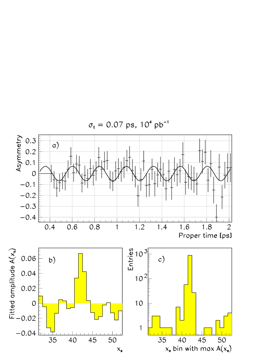
Figure 4: $x_{s}=42$, ”nominal” parameters: $\sigma_{t}=0.07$ ps and $\int Ldt=\mathrm{1}0^{4}\ pb^{-1}$; (a) time-dependent asymmetry distribution (single experiment), (b) amplitude $A(x_{s})$ fitted to the distribution shown in (a), (c) distribution of $x_{s}$ giving the highest value of $A(x_{s})$ when the experiment was repeated 1000 times.

For ATLAS, with the parameters listed in section 2.1 the limit turns out to be $x_{s}^{max}=42$. A time-dependent asymmetry distribution, its transformation with the amplitude fit procedure and the results of 1000 simulated experiments are shown in Fig.4.

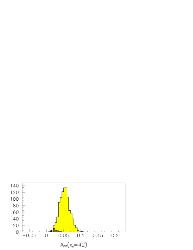
Figure 5: Distribution of the amplitudes fitted for $x_{s}=42$ for 1000 ’experiments’ (generated with the ’true’ $x_{s}=42$). Dark histogram shows amplitudes for 31 ’experiments’ which ’fail’.

For the correct frequency an average amplitude should be equal to the product of all dilution factors $D$ (see formula 1). Figure 5 shows the distribution of the fitted amplitudes. An average value $(53.15\pm 0.49)\cdot 10^{-3}$ is in agreement with the prediction from formulas 2 to 5 equal $D=52.85\cdot 10^{-3}$.

3 Dependence of the range on $\sigma_{t}$ and on integrated luminosity

In order to evaluate the importance of the proper time resolution $\sigma_{t}$ and of the integrated luminosity, the analysis was repeated for different values of these parameters. All combinations given by $\sigma_{t}$ values of 0.05, 0.07, 0.09 and 0.11 ps, together with $\int Ldt$ values of 0.5, 1.0, 2.0, 5.0 and $10.0\times\mathrm{1}0^{4}\ pb^{-1}$ were tried.

Figure 6: $x_{s}=27$, $\sigma_{t}=0.11$ ps and $\int Ldt=\mathrm{1}0^{4}\ pb^{-1}$; (a) time-dependent asymmetry distribution (single experiment), (b) amplitude $A(x_{s})$ fitted to the distribution shown in (a), (c) distribution of $x_{s}$ giving the highest value of $A(x_{s})$ when the experiment was repeated 1000 times.

Deteriorating the proper time resolution form the ’nominal’ 0.07 ps to 0.11 ps reduces the $x_{s}^{max}$ to 27, as could be expected from formula 6. The corresponding summary plot is shown in figure 6.

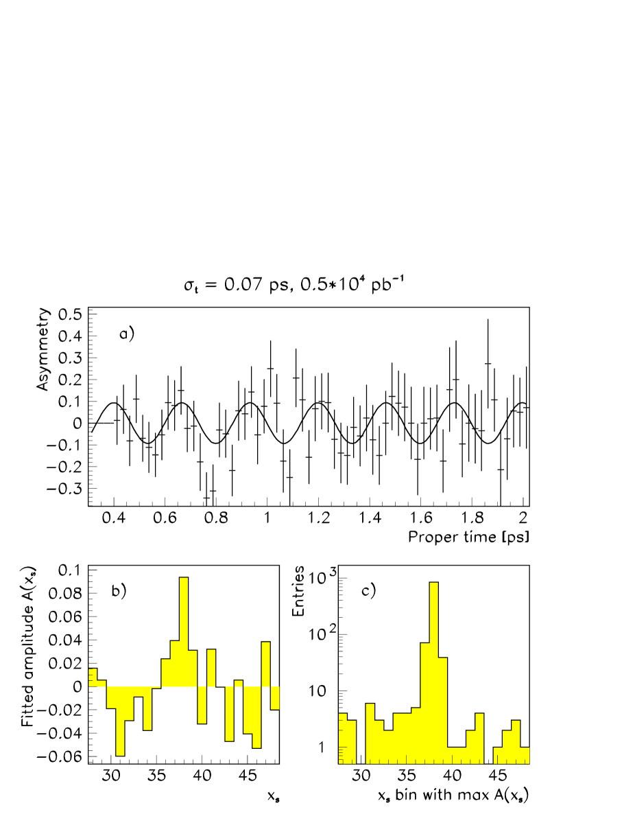
Figure 7: $x_{s}=38$, $\sigma_{t}=0.07$ ps and $\int Ldt=0.5\cdot\mathrm{1}0^{4}\ pb^{-1}$; (a) time-dependent asymmetry distribution (single experiment), (b) amplitude $A(x_{s})$ fitted to the distribution shown in (a), (c) distribution of $x_{s}$ giving the highest value of $A(x_{s})$ when the experiment was repeated 1000 times.

If $\sigma_{t}$ has the nominal value and the integrated luminosity is reduced to $0.5\cdot\mathrm{1}0^{4}\ pb^{-1}$ the $x_{s}^{max}$ is less reduced: $x_{s}^{max}=38$ (see figure 7).

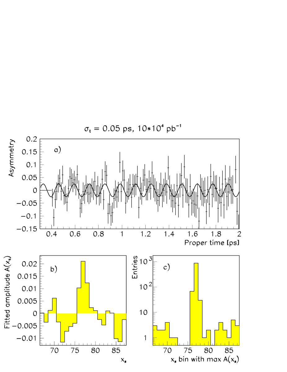
Figure 8: $x_{s}=77$, $\sigma_{t}=0.05$ ps and $\int Ldt=10\cdot\mathrm{1}0^{4}\ pb^{-1}$; (a) time-dependent asymmetry distribution (single experiment), (b) amplitude $A(x_{s})$ fitted to the distribution shown in (a), (c) distribution of $x_{s}$ giving the highest value of $A(x_{s})$ when the experiment was repeated 1000 times.

A full scan of the two parameters also gives a set of values: $\sigma_{t}=0.05$ ps and $\int Ldt=10^{5}{\mathrm{p}b}^{-1}$. Such a combination gives $x_{s}^{max}=77$ (Fig. 8).

Figure 9: Sensitivity range of the ATLAS experiment for the $x_{s}$ measurement, as a function of the proper-time resolution $\sigma_{t}$, for various integrated luminosities. The points come from Monte-Carlo calculations, the solid lines show $1/\sigma_{t}$ dependence.

A summary plot showing the $x_{s}^{max}$ versus $\sigma_{t}$ for various integrated luminosities is shown in figure 9. The expected dependence given by the formula 6, shown with solid lines in the figure, is well confirmed.

Figure 10: Sensitivity range of the ATLAS experiment for the $x_{s}$ measurement, as a function of the integrated luminosity, for various proper-time resolutions $\sigma_{t}$. The points come from Monte-Carlo calculations, the solid lines show the $x_{s}^{max}\simeq(2.90/\sigma_{t})\cdot(1+0.15\ln(\int Ldt))$ parametrisation, where $\sigma_{t}$ is in ps and $\int Ldt$ is in units of $\mathrm{1}0^{4}\ pb^{-1}$ .

The same summary in another projection, $x_{s}^{max}$ versus $\int Ldt$ for different values of $\sigma_{t}$, is shown in figure 10. It is found, that the ATLAS range for the $x_{\mathrm{s}}~{}$measurement can be parameterized in the following way:

$$x_{s}^{max}\simeq\frac{2.90}{\sigma_{t}}\left[{1+0.15\ln\left({\int Ldt}\right)}\right]$$ (7)

where $\sigma_{t}$ is given in ps and $\int Ldt$ in units of $\mathrm{1}0^{4}\ pb^{-1}$ . The solid lines in figure 10 show the prediction of the above formula.

4 Dependence on signal-to-background ratio

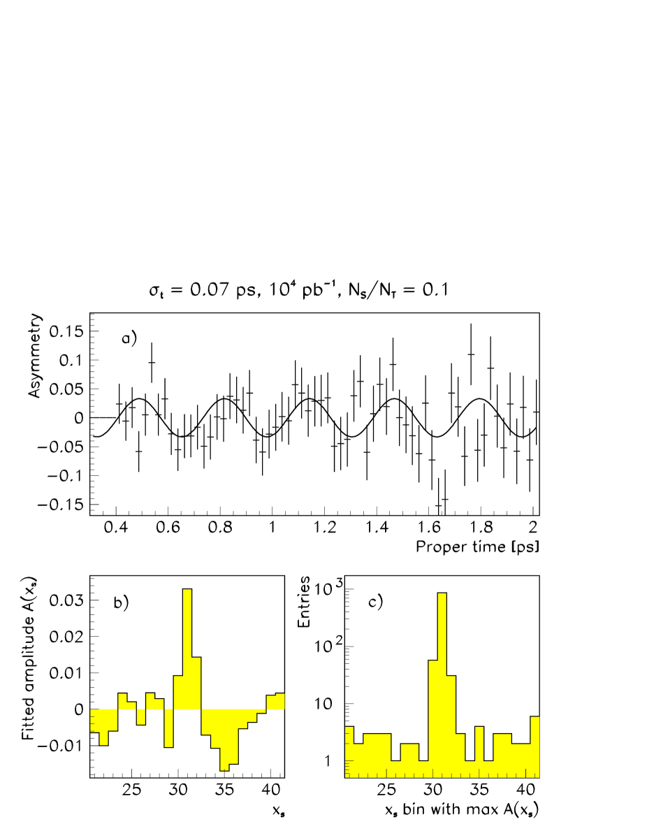
Figure 11: $x_{s}=31$, $\sigma_{t}=0.07$ ps and $\int Ldt=\mathrm{1}0^{4}\ pb^{-1}$, $N_{B}/N_{S}=1.0$; (a) time-dependent asymmetry distribution (single experiment), (b) amplitude $A(x_{s})$ fitted to the distribution shown in (a), (c) distribution of $x_{s}$ giving the highest value of $A(x_{s})$ when the experiment was repeated 1000 times.

The scan of parameters $\sigma_{t}$ and $\int Ldt$ described in the previous section was done for the background-to-signal ratio of 1. By increasing the number of background events such that $N_{S}/(N_{B}+N_{S})$ becomes equal 0.1 we reduce $x_{s}^{max}$ to 31 for the ’nominal’ parameters $\sigma_{t}=0.07$ ps and $\int Ldt=\mathrm{1}0^{4}\ pb^{-1}$ (see figure 11).

Figure 12: Sensitivity range of the ATLAS experiment for the $x_{s}$ measurement, as a function of the signal content of the sample, for $\sigma_{t}=0.07$ ps and $\int Ldt=\mathrm{1}0^{4}\ pb^{-1}$.

A summary plot showing the dependence of $x_{s}^{max}$ on background is shown in figure 12. $N_{S}$ was kept constant at its predicted value for $\int Ldt=\mathrm{1}0^{4}\ pb^{-1}$ ($N_{S}=4480$, see section 2.1), while the number of background event was varied between $N_{B}=0$ and $N_{B}=9\times N_{S}$. It can be observed, that the dependence of $x_{s}^{max}$ on background is not strong. It should be noted however, that background had no asymmetry in the simulation and a simple exponential dependence $dN_{B}/dt\sim\exp(-t/\tau)$ was assumed.

5 Conclusions

It is justified theoretically, after [4], that the sensitivity range $x_{s}^{max}$ is proportional to $1/\sigma_{t}$ (where $\sigma_{t}$ is the resolution in the B-decay proper time), for any given integrated luminosity and signal-to-background ratio, independently of the method of defining the sensitivity range.

With the methods described in section 2 it is found that $x_{s}^{max}=42$ for nominal ATLAS parameters. The Monte-Carlo study done for various integrated luminosities and for different $\sigma_{t}$ values shows, that ATLAS sensitivity range can be parameterized as $x_{s}^{max}\simeq(2.90/\sigma_{t})\cdot(1+0.15\ln(\int Ldt))$, where $\sigma_{t}$ is in ps and $\int Ldt$ is in units of $\mathrm{1}0^{4}\ pb^{-1}$. It is also found, that the dependence of $x_{s}^{max}$ on background is relatively weak.

References

- [1] C. Zeitnitz, in the proceedings of the Beauty’96 Conference, held in Rome June 17-21, 1996. To be published in Nucl. Instrum. and Methods A.
- [2] P. Eerola, S. Gadomski, B. Murray ‘ mixing measurement in ATLAS’, ATLAS Internal Note, PHYS-NO-39, 16 June 1994, Available on WWW (http://atlasinfo.cern.ch/Atlas/GROUPS/PHYSICS/NOTES/notes.html)
- [3] A. V. Bannikov, G. A. Chelkov, Z. K. Silagadze ‘ decay channel in the -mixing studies’, ATLAS Internal Note, PHYS-NO-072, 10 October 1995, Available on WWW (http://atlasinfo.cern.ch/Atlas/GROUPS/PHYSICS/NOTES/notes.html)
- [4] H.-G. Moser, A. Roussarie ‘Mathematical methods for Oscillation Analyses’, ALEPH preprint 14 May 1996, submitted to NIM, available on WWW (http://alephwww.cern.ch/ALPUB/pub/pub.html)
- [5] The ATLAS collaboration, ATLAS technical proposal, CERN/LHCC/94-43, LHCC/P2, 15 December 1994.
- [6] ’Particles and Fields’, Physical Reviev D 54, 1 July 1996.
- [7] P. Eerola, presentation during the ATLAS Inner Detector Working Group meeting, June 26th, 1996.
- [8] R. Forty ’Lifetimes of heavy flavour particles’, CERN-PPE/94-144 (1994).