FERMILAB-CONF-96/162-E

Jet Decorrelation and Jet Shapes at the Tevatron

Terry C. Heuring

Florida State University
(for the DØ Collaboration)

We present results on measurements of jet shapes and jet azimuthal decorrelation from $\overline{p}p$ collisions at $\sqrt{s}=1.8$ TeV using data collected during the 1992–1993 run of the Fermilab Tevatron. Jets are seen to narrow both with increasing $E_{T}$ and increasing rapidity. While HERWIG, a parton shower Monte Carlo, predicts slightly narrower jets, it describes the trend of the data well; NLO QCD describes qualitative features of the data but is sensitive to both renormalization scale and jet definitions. Jet azimuthal decorrelation has been measured out to five units of pseudorapidity. While next–to–leading order QCD and a leading–log approximation based on BFKL resummation fail to reproduce the effect, HERWIG describes the data well.

1 Introduction

As progress has extended perturbative quantum chromodynamics (QCD) beyond leading order, theoretical comparisons of a more detailed nature are being performed with experimental data. The advent of both next–to–leading order (NLO) and leading–log approximations (LLA) has enabled predictions for both event topologies involving more than two jets and the internal structure within a jet. This paper reports on two such studies, one involving a detailed examination of the transverse energy flow within jets and the other involving the first study of azimuthal decorrelation of jets with large separations in pseudorapidity.

In both studies, NLO QCD is the first order in which a theoretical prediction is possible. Although NLO predictions have been successful in describing inclusive single jet and dijet [1] cross sections, deviations from the measured distributions or a large sensitivity to the choice of renormalization scale may indicate large higher order corrections. In this case, an all–orders approximation in the form of a LLA may produce better results. For the jet shape analysis, a model where only one additional radiated parton is allowed may prove inadequate to reproduce all aspects of the transverse energy flow. Additional fragmentation effects may indeed be important. In jet production with large rapidity separations, the presence of multiple scales in the calculation may require a resummation. Two alternative methods are explored, one resumming $\ln Q^{2}$ via DGLAP [2] splitting functions and the other resumming $\ln(\hat{s}/Q^{2})$ using the BFKL [3] equation. A comparison of experimental results to theoretical predictions will determine the necessity of including such higher order corrections.

2 Jet Shape

The data for this study [4] were collected using the DØ detector which is described in detail elsewhere [5]. The critical components for this study are the uranium–liquid argon calorimeters. These calorimeters provide hermetic coverage over most of the solid angle with a transverse segmentation of $0.1\times 0.1$ in $\eta\times\phi$ ($\eta=-\ln[\tan(\theta/2)]$, where $\theta$ is the polar angle with respect to the proton beam and $\phi$ is the azimuthal angle). The measured resolutions are $15\%/\sqrt{E}$ and $50\%/\sqrt{E}$ (E in GeV) for electromagnetic and single hadronic showers respectively.

The data were collected using four separate triggers, each requiring a minimum $E_{T}$ in a specified number of trigger towers ($0.2\times 0.2$ in $\eta\times\phi$) at the hardware level. Events satisfying these requirements were sent to a processor farm where a fast version of the offline jet algorithm searched for jet candidates above some $E_{T}$ threshold. These events were used to populate four non-overlapping jet $E_{T}$ ranges: 45-70, 70-105, 105-140, and $>140$ GeV. Each trigger was used only where it was fully efficient.

Jets were reconstructed offline using an iterative fixed cone algorithm with a radius R = 1.0 in $\eta-\phi$ space. The final jet angles were defined as follows: $\theta_{\rm jet}=\tan^{-1}\sqrt{(\Sigma_{i}E_{xi})^{2}+(\Sigma_{i}E_{yi})^{2})}/\Sigma_{i}E_{zi}$ and $\phi_{\rm jet}=\tan^{-1}(\Sigma_{i}E_{yi}/\Sigma_{i}E_{xi})$ with $z$ in the beam direction and the sums extending over calorimeter towers whose centers were contained within the jet cone. These definitions differ from the Snowmass algorithm [6]: $\eta_{\rm jet}=\Sigma_{i}E_{Ti}\eta_{i}/\Sigma_{i}E_{Ti}$ and $\phi_{\rm jet}=\Sigma_{i}E_{Ti}\phi_{i}/\Sigma_{i}E_{Ti}$. In both cases, the $E_{T}$ of the jet was defined as $\Sigma_{i}E_{Ti}$. After a preliminary set of jets was found, overlapping jets were redefined. Two jets were merged into one jet if more than 50% of the $E_{T}$ of the jet with the smaller $E_{T}$ was contained in the overlap region. The direction of the new jet was defined as the vector sum of the two original jet momenta, and the energy was recalculated. If less than 50% of the $E_{T}$ was contained in the overlap region, the jets were split into two distinct jets. In this case, the energy of each calorimeter cell in the overlap region was assigned to the nearest jet and the jet directions were recalculated. Two different $\eta$ regions ($|\eta|<0.2$ and $2.5<|\eta|<3.0$) were studied.

For this study we define the quantity $\rho(r)=(1/N_{\rm jets})\Sigma_{\rm jets}E_{T}(r)/E_{T}(r=1)$ ($N_{\rm jets}$ is the number of jets in the sample) which is the average fraction of the jet transverse energy contained in a subcone of radius $r$. For a given value of $r$, a larger value of $\rho$ represents a narrower jet. Individual subcones were corrected for underlying event and noise effects only.

In Fig. 1, the average $E_{T}$ fraction ($\rho$) versus the subcone radius is shown for the two different $\eta$ regions for jets between 45 and 70 GeV $E_{T}$. Also shown in this figure are the predictions from HERWIG [7], a Monte Carlo prediction which incorporates higher order effects through a parton shower model. Detector effects were modeled using a detailed detector simulation based on GEANT [8]. Although properly describing the qualitative behavior of the data, in both the central and forward regions the theoretical predictions are narrower than the measured jet shapes. In order to remove detector effects, correction factors were determined using three different event generators, comparing the jet shape before and after detector simulation. In the subsequent distributions, the detector effects have been removed using these correction factors.

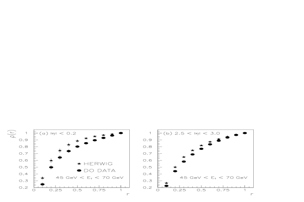
Figure 1: The average integrated $E_{T}$ fraction versus the subcone radius is plotted for the data and HERWIG Monte Carlo, before calorimetric effects are removed, for the $E_{T}$ range 45-70 GeV for (a) $|\eta|\leq 0.2$ and (b) $2.5\leq|\eta|\leq 3.0$.

Figure 2: The measured jet shapes, with calorimetric effects removed, compared to NLO predictions (JETRAD) with three renormalization scales for $|\eta|\leq 0.2$ for the jet $E_{T}$ range (a) 45-70 GeV, (b) 70-105 GeV, (c) 105-140 GeV, (d) greater than 140 GeV.

In Fig. 2, the jet shape for the four different $E_{T}$ regions are shown for central jets ($|\eta|<0.2$). We see that as the $E_{T}$ of the jet increases, a larger fraction of its total $E_{T}$ is contained in the inner subcones, i.e. the jets are narrower. This result is in good agreement with CDF [9] measurements (Fig. 3) where jet shapes were determined using charged particle tracks only. In Fig. 4, the jet shape for a single $E_{T}$ range in both the central and the forward $\eta$ region is shown. We see that jets of the same $E_{T}$ become narrower as the jets become more forward.

Figure 3: A comparison of the DØ and CDF jet shapes. The CDF measurement was made using charged tracks only for $0.1<|\eta|<0.7$ and average $E_{T}=100$ GeV. The two DØ measurements ($|\eta|\leq 0.2$), with detector effects removed, were made at $E_{T}$’s above and below that of CDF. Good agreement is seen.

Figure 4: Comparisons of jet shapes from data and NLO predictions using different jet direction definitions for jets with $70<E_{T}<105$ and for (a) $|\eta|\leq 0.2$ and (b) $2.5\leq|\eta|\leq 3.0$.

Also shown in Figs. 2 and 4 is a comparison to NLO QCD predictions made with JETRAD [10] using CTEQ2M [11] parton distribution functions (pdf) and three different renormalization scales($\mu$): $2E_{T}$, $E_{T}$, and $E_{T}/2$. Studies showed the theoretical predictions were insensitive to choices in pdf. Since this is a NLO QCD prediction containing at most three partons in the final state, jet shape arises from combining two final state partons into one jet. For this study, two partons were considered to constitute one jet if their distance in $\eta$ – $\phi$ space from their vector sum was less than one. Using the DØ definitions of jet angles, central jets are found to be generally wider than predicted by JETRAD. Forward jets are narrower than predicted and the observed narrowing of forward jets with increasing $E_{T}$ is not reproduced by JETRAD.

As shown in Fig. 4, using the Snowmass definition of jet angles generally improves the agreement between data and predictions. While the experimental jet shape distribution is only moderately affected by the choice of jet angle definition, the theoretical prediction in the forward region is very sensitive to this choice. Qualitatively, the NLO calculations using the Snowmass algorithm describe the measured jet shapes reasonably well. However, these predictions, being the first order in which a nontrivial jet shape emerges, show large sensitivity to the choice of renormalization scale with no single choice able to describe the data at all $E_{T}$’s.

3 Jet Azimuthal Decorrelation

In this study [12] we are interested in jets widely separated in pseudorapidity and at relatively low $E_{T}$. By measuring the $\phi$ correlation of the dijet system we gain information about the radiation pattern in the event. The data used for this study were collected in a similar fashion to the jet shape study. In this case, a single trigger was used. It required $E_{T}>7$ GeV at the hardware level and searched for jet candidates with an $E_{T}$ threshold of 30 GeV in the processor farm. Offline, jets were reconstructed using an iterative fixed cone algorithm with a radius of R = 0.7 in $\eta-\phi$ space. Both the final jet angles and the merging and splitting criteria were defined as described above.

From the sample of jets collected with $E_{T}>20$ GeV and $|\eta|<3.0$, the two jets at the extremes of pseudorapidity were selected. To remove any trigger inefficiencies, one of these two jets was required to have $E_{T}>50$ GeV. The relevant quantities used in this analysis are $\Delta\eta=|\eta_{1}-\eta_{2}|$ and $\Delta\phi=\phi_{1}-\phi_{2}$ (where the subscripts refer to the two jets described above).

Figure 5: The pseudorapidity interval, $\Delta\eta=|\eta_{1}-\eta_{2}|$, of the two jets at the extremes of pseudorapidity. The coverage extends to $\Delta\eta\sim 6$. The errors are statistical only.

Figure 6: The azimuthal angle difference, $\Delta\phi=\phi_{1}-\phi_{2}$, distribution of the two jets at the extremes of pseudorapidity plotted as $1-\Delta\phi/\pi$ for $\Delta\eta=$ 1, 3, and 5. The errors are statistical only.

Since the trigger was implemented out to $|\eta|<3.0$, the maximum value of $\Delta\eta$ is $\sim 6.0$. This is illustrated in Fig. 6 where we plot the pseudorapidity interval $\Delta\eta$ for events passing our cuts. In Fig. 6, the azimuthal angular separation, $1-\Delta\phi/\pi$ is plotted for three selected unit bins of $\Delta\eta$ centered at $\Delta\eta=$ 1, 3, and 5. The correlation of the two jets at the extremes in pseudorapidity is evident in the shape of this distribution which becomes wider (less correlated) at $\Delta\eta$ increases. A correlation variable, $\langle\cos(\pi-\Delta\phi)\rangle$, has been defined to study the effect quantitatively. This quantity is plotted in Fig. 7 as a function of $\Delta\eta$. For the data, the error bars represent the statistical and uncorrelated systematic errors added in quadrature. An error band at the bottom of the plot represents the correlated systematic error due to the energy scale and detector effects. Also shown in Fig. 7 are the theoretical predictions from HERWIG, NLO QCD as implemented in JETRAD, and BFKL resummation [13]. The errors for the predictions are statistical only.

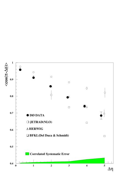
Figure 7: The correlation variable used in this analysis, $\langle\cos(\pi-\Delta\phi)\rangle$ vs. $\Delta\eta$, for the data, JETRAD, HERWIG, and the BFKL calculations of Del Duca and Schmidt.

For the data, many sources of systematic error were investigated. For all values of $\Delta\eta$ the energy scale error dominates, except for $\Delta\eta=5$, where the measurement is statistically limited. Other systematic errors due to the out–of–cone showering correction, angular biases present in the jet reconstruction, and our selection cuts are included. Although no attempt was made to correct back for detector effects, the size of any such effects was estimated using HERWIG events that were subjected to a detailed simulation of our detector based on GEANT. The size of the effect was negligible for $\Delta\eta\leq 3$ and only $\sim 0.03$ at $\Delta\eta=5$ and are included in the systematic correlated error band.

Systematic effects were also studied in the theory. The renormalization and factorization scale $\mu$ was varied in the NLO prediction from $\mu=p_{T}^{max}/2$ to $2p_{T}^{max}$. The largest variation seen in $\langle\cos(\pi-\Delta\phi)\rangle$ was less than 0.026. Different parton distribution functions were used (CTEQ2M, MRSD$-$ [14], and GRV [15]) resulting in variations of less than 0.003. In addition, the Monte Carlo study was repeated using the Snowmass jet angle definitions. The difference in $\langle\cos(\pi-\Delta\phi)\rangle$ was less than 0.013. As a cross check, a subset of the data was analyzed using the Snowmass jet angle definitions as well. The resulting variations were less than 0.002.

The data in Fig. 7 show a nearly linear decorrelation effect with pseudorapidity. For small $\Delta\eta$ both HERWIG and JETRAD describe the data well. However, at large $\Delta\eta$ JETRAD, which is leading order in describing any decorrelation effect, shows deviations from the measurement predicting too little decorrelation. The BFKL predictions, valid for large $\alpha_{s}\Delta\eta$, are shown for $\Delta\eta\geq 2$. As the pseudorapidity interval increases, this leading–log approximation predicts too much decorrelation. The HERWIG prediction, which includes higher order processes in the form of a parton shower model including angular ordering, describes the data well over the entire $\Delta\eta$ region.

4 Conclusion

We have presented results on both jet shapes and azimuthal decorrelation in dijet systems. These results have been compared to various theoretical predictions. We see that jets become narrower as their $E_{T}$ increases for a fixed $\eta$ and that they become narrower as their $\eta$ increases for fixed $E_{T}$. The measured jet shapes are insensitive to jet angle definitions while the NLO QCD predictions are sensitive to jet angle definition. Reasonable behavior is seen when Snowmass jet angle definitions are used. We see that the dijet systems decorrelate in a linear fashion out to $\Delta\eta=5$. Comparisons to various theoretical predictions show that NLO QCD predicts too little while BFKL resummation predicts too much decorrelation. HERWIG reproduces the data over the entire $\Delta\eta$ range explored.

References

-
[1]
G. Blazey (DØ Collaboration), in the proceedings of the XXXIst
Recontres de Moriond, March 1996;
CDF Collaboration, F. Abe et al., Phys. Rev. Lett., 69 2896, (1992). -
[2]
V.N. Gribov and L.N. Lipatov, Sov. J. Nucl. Phys. 46, 438 (1972);
L.N. Lipatov, Sov. J. Nucl. Phys. 20, 95 (1975);
G. Altarelli and G. Parisi, Nucl. Phys. B126, 298 (1977);
Yu.L. Dokshitzer, Sov. Phys. JETP 46, 641 (1977). -
[3]
L.N. Lipatov, Sov. J. Nucl. Phys. 23, 338 (1976);
E.A. Kuraev, L.N. Lipatov, V.S. Fadin, Sov. Phys. JETP 44, 443 (1976); Sov. Phys. JETP 45, 199 (1977);
Ya.Ya. Balitsky, L.N. Lipatov, Sov. J. Nucl. Phys. 28, 822 (1978). - [4] DØ Collaboration, S. Abachi et al., Phys. Lett. B357 500 (1995).
- [5] DØ collaboration, S. Abachi et al., Nucl. Instrum. Methods A338, 185 (1994).
- [6] J. Huth et al., in proceedings of Research Directions for the Decade, Snowmass 1990, edited by E.L. Berger (World Scientific, Singapore, 1992).
-
[7]
G. Marchesini, B.R. Webber, Nucl. Phys. B310, 461 (1988);
I.G. Knowles, Nucl. Phys. B310, 571 (1988);
G. Marchesini et al., Comp. Phys. Comm. 67, 465 (1992). - [8] R.Brun et al., “GEANT3.14” (unpublished), CERN, DD/EE/84-1.
- [9] CDF Collaboration, F. Abe et al, Phys. Rev. Lett., 70, 713 (1993).
- [10] W.T. Giele, E.W.N. Glover and D.A. Kosower, Nucl. Phys. B403, 633 (1993).
-
[11]
CTEQ Collaboration, J. Botts, et al.,
Phys. Lett. B304, 159 (1993);
W.K. Tung, in the Proceedings of the International Workshop on Deep Inelastic Scattering and Related Subjects, Eilat, Israel (World Sci., Singapore, 1994). - [12] DØ Collaboration, S. Abachi et al., to be published in Phys. Rev. Lett. (hep-ex/9603010).
- [13] V. Del Duca, C.R. Schmidt, Phys. Rev. D 51, 2150 (1995); Phys. Rev. D 49, 4510 (1994).
- [14] A.D. Martin, W.J. Stirling, R.G. Roberts, Phys. Rev. D 47, 867 (1993).
- [15] A. Vogt, Phys. Lett. B 354, 145 (1995).