Abstract

We describe the anticipated experimental program of an $e^{+}e^{-}$ linear collider in the energy region 500 GeV–1.5 TeV, emphasizing topics relevant to the mystery of electroweak symmetry breaking.

 

1 INTRODUCTION

Elementary particle physics has always progressed by attacking its mysteries simultaneously from many different directions. The parton model of hadronic structure, for example, was developed both in response to the discovery of limited transverse momentum in high-energy hadron collisions and to the discovery of scaling in deep-inelastic electron scattering. As particle physics has moved to increasingly high energies, however, the accelerators needed to reach these energies have become progressively more expensive. Thus our community has needed to consolidate its efforts into the most promising channels. It is inevitable that this consolidation will continue into the future.

But, it spite of this, it will continue to be important that experiments confront new phenomena from distinct and complementary perspectives. The exploration of the 100-GeV mass scale has been carried out by proton-antiproton experiments at CERN and Fermilab, electron-positron annihilation experiments at SLAC and CERN, and electron-proton scattering experiments at DESY. All of these experiments have contributed pieces to the major result, the precise confirmation of the standard model of electroweak interactions. In the future, as we explore the 1 TeV mass scale, we hope that proton-proton and electron-positron collider experiments will both be available.

A proton-proton collider appropriate to this task, the LHC at CERN [1], has already been approved. The major physics goals of $pp$ experiments at TeV energies have been summarized in many places, including earlier contributions to this series [2, 3], the physics chapters of the LHC detector technical proposals [4, 5], and the classic review paper [6]. In this article, we will present the corresponding review of the major goals of $e^{+}e^{-}$ experimentation at the next step of high energy. Our discussion will emphasize the unique capabilities of $e^{+}e^{-}$ reactions, and the aspects in which $e^{+}e^{-}$ experiments complement the capabilities of $pp$ colliders.

In the past few years, there have been a number of international conferences on physics of $e^{+}e^{-}$ linear colliders whose proceedings are valuable sourcebooks [7, 8, 9, 10, 11]. In addition, a set of useful review articles on future colliders have been prepared for a recent study commissioned by the Division of Particles and Fields of the American Physical Society [12]. Part of our task will be to survey the information contained in these volumes.

1.1 ‘Beyond the Standard Model’

In principle, one could discuss the physics goals of a proposed accelerator simply by listing the various reactions it can produce and enumerating the possible results to be obtained from each. In this review, we will take a more focused viewpoint. The physics of the 100 GeV–1 TeV mass scale is still largely unexplored territory, but it is not the complete mystery that, for example, the asymptotic behavior of the strong interactions was in 1960. We are guided in our approach to this region by the dramatic success of the standard model of strong, weak, and electromagnetic interactions, and by the questions that this model reserves to higher energies. Indeed, we take the position that there is a single most crucial problem to be solved by the next generation of accelerators—to find the mechanism for the spontaneous breaking of the electroweak gauge symmetry. In our opinion, any proposal for a new accelerator must ultimately justify itself by its ability to uncover crucial clues to this problem.

What gives this particular problem such importance? The first reason is the contrast between our detailed knowledge of the gauge couplings of the standard model and our ignorance of the physics of mass generation. The Glashow-Weinberg-Salam $SU(2)\times U(1)$ theory of electroweak interactions is now tested at the tenth-percent level, most dramatically in the experimental determination of the $Z^{0}$ partial widths and asymmetries at LEP and SLC. [14, 15] These experiments directly test the central assumptions of the $SU(2)\times U(1)$ model. They show that the left- and right-handed components of the quarks and leptons have completely different couplings to the fundamental electroweak gauge bosons. Thus, these components must be viewed as distinct species at high energy. At the same time, they show that the weak interaction coupling constants are universal among species. This strongly suggests that the electroweak bosons are the vector bosons of a gauge theory. These two facts imply that neither the elementary fermions nor the elementary vector bosons can obtain mass without the spontaneous breaking of the gauge symmetry. However, the $SU(2)\times U(1)$ model does not contain a physical mechanism for breaking its own symmetry, since the electroweak interactions are weakly coupled. Some external agent, a new particle or sector of particles, is required.

Second, the physics of this new sector should be very close at hand, at an energy scale within the reach of the next generation of accelerators. The gauge relations of the $SU(2)\times U(1)$ model give for the $W$ boson mass a formula $m_{W}={1\over 2}gv$, where $g$ is the $SU(2)$ gauge coupling and $v$ is a mass scale characteristic of the spontaneous symmetry breaking. In the simplest model, in which the gauge symmetry is broken by the expectation value of a single scalar field, $v$ is the size of this vacuum expectation value. From the known values of the $W$ mass and the $SU(2)$ gauge coupling, we have

$$v=250\ \hbox{\rm GeV}\ .$$ (1)

This scale should set at least the order of magnitude for the masses of the new particles which cause electroweak symmetry breaking. To find the detailed relation between $v$ and these masses, one must study explicit models of electroweak symmetry breaking, and the answer is somewhat model-dependent. Nevertheless, it is true in all but the most extreme models that these particles are accessible to a $pp$ collider at 14 TeV in the center of mass and to an $e^{+}e^{-}$ collider at 1.5 TeV in the center of mass.

Finally, the physics of electroweak symmetry breaking is important because it enters into the discussion of all of the other fundamental problems of the theory of elementary particles. We have already explained that this symmetry breaking is crucial for the generation of quark and lepton masses, so any explanation of the fermion mass spectrum, and the related problems of the origin of the quark mixing angles and $CP$ violation, must begin by assuming a specific mechanism of electroweak symmetry breaking. The same conclusion holds for problems less obviously connected to mass generation. Consider, for example, the possibility of lepton number violation observed in the process $\mu\to e\gamma$. If this process were observed, it would be a spectacular discovery, but its implications for the broader theory of Nature would be left obscure. Models of $\mu\to e\gamma$ include ones based on heavy neutral leptons [16], on extended technicolor [17], and on supersymmetric grand unification [18]. The broad classes of models for this process, or any similar exotic process, are distinguished precisely by their assumptions about the physics of electroweak symmetry breaking. So it is not enough to search for anomalies; even to understand the consequences of these searches, we must go to the electroweak scale and see what is there.

This review will be organized around the ability of a proposed $e^{+}e^{-}$ collider to study the implications of various models of electroweak symmetry breaking. We begin in Sections 2 by providing background material on the accelerator and detector designs for these colliders. In Sections 3 and 4, we discuss two exotic standard-model reactions that will be explored in detail at this collider, $e^{+}e^{-}\to W^{+}W^{-}$ and $e^{+}e^{-}\to t\overline{t}$. Both of these reactions have unusual features that should already provide an interesting experimental program, but they are only a prelude to the real interest of this machine in studying the electroweak scale.

In Sections 5–7, we discuss specific models of electroweak symmetry breaking and their experimental consequences at $e^{+}e^{-}$ colliders. Models of electroweak symmetry breaking divide generally into two classes—those models in which the physics is essentially weak-coupling, and those in which this physics is strong-coupling. In models of the first class, the electroweak symmetry is broken by the vacuum expectation value of an elementary scalar field, called the Higgs field. The simplest model contains only one Higgs field, and one new particle, the Higgs boson. This theory is sometimes dignified with the title “the minimal standard model,” but it is not really a model at all; it does not explain electroweak symmetry breaking and it cannot naturally be incorporated into a unified model of the fundamental interactions. More general models can be built with several Higgs fields and many more free parameters. However, the only models of this type that are conceptually coherent and also have the power to explain electroweak symmetry breaking are those that incorporate an additional symmetry, called supersymmetry. In this case, the experimental signatures can be fully worked out and capabilities of various collider options discussed quantitatively. In Section 5, we will discuss experiments at an $e^{+}e^{-}$ collider on the Higgs boson and its possible scalar counterparts. In Section 6, we will discuss experiments on the additional new particles predicted by supersymmetry.

In Section 7, we will turn to the second class of models in which electroweak symmetry breaking is caused by new strong-coupling dynamics at the TeV scale. These models do not contain elementary Higgs fields at all but instead postulate new forces that lead to electroweak symmetry breaking. Because of their strong interactions, it is difficult in this case to completely predict the properties of the model; thus, many aspects of phenomenology must be discussed in a qualitative way. However, we can still provide an overview of the variety of experimental signatures available.

Finally, in Section 8, we give a lightning review of other models of new physics that can be tested at $e^{+}e^{-}$ colliders.

1.2 Special Features of $e^{+}e^{-}$ Experimentation

As an introduction to this review, we will discuss in this section three general features of the experimental environment provided by $e^{+}e^{-}$ annihilation. Electron-positron colliders played a major role in the discoveries of the 1970’s and the confirmation of the standard model in the 1980’s because they offer to experimenters a number of aspects that simplify the investigation of exotic phenomena. We will argue in this review that these features, which are familiar from $e^{+}e^{-}$ experiments at present energies, should also be present in the $e^{+}e^{-}$ experiments of the future.

The first of these features is what is often called the “cleanliness” of $e^{+}e^{-}$ reactions, the fact that standard-model event rates are relatively low. At high energy, two somewhat different aspects of the standard model processes are important, that these processes have relatively simple topology, and that their rates are precisely calculable. The standard-model background processes with the largest cross sections are photon-photon collisions and radiative annihilation processes ($e^{+}e^{-}\to q\overline{q}\gamma$); however, these processes are eliminated by simple cuts on total visible energy and energy balance. The annihilation process $e^{+}e^{-}\to q\overline{q}$ is eliminated equally simply by removing two-jet-like events. This leaves as the dominant backgrounds for exotic processes reactions that themselves involve heavy species, in particular, $e^{+}e^{-}\to W^{+}W^{-}$ and $e^{+}e^{-}\to t\overline{t}$. We will see that this is the normal situation in the specific analyses to be discussed below. General studies of background levels at linear collider energies are reviewed, for example, in [19, 20, 21], and, briefly, in section 2.2.

The second general feature of $e^{+}e^{-}$ annihilation is one that we might call “democracy.” The typical values of cross sections in $e^{+}e^{-}$ annihilation are set by the point cross section

$$1\ \hbox{\rm R}={4\pi\alpha^{2}\over 3s}={86.8\ \hbox{\rm fb}\over(E_{\hbox{\scriptsize CM}}\ \hbox{\rm(TeV)})^{2}}\ .$$ (2)

As long as a given process is kinematically allowed, its cross section will be of order 1 R times the squares of gauge charges. Thus, exotic processes typically occur at the rates of standard-model process. On the other hand, the point cross section given in Eq. 2 is rather small, and this poses a challenge to accelerator designers.

The third general feature of $e^{+}e^{-}$ annihilation is one that we (being Californians) might call “holism,” the fact that typically the complete event is captured, so that its full kinematic information can be used. In any study of new physics processes at TeV energies, it is typical that both the signal and the dominant background processes will contain $W$ bosons. If these $W$ bosons can be reconstructed, their decay distributions indicate their polarizations, and this polarization information can become an important ingredient in the analysis. We will discuss several examples in which the decay distributions of heavier particles also come into play. In addition, $e^{+}e^{-}$ colliders offer the freedom to adjust the electron polarization and the availability of $b$-quark tagging with high efficiency. We will see how all of these handles can work together to detect and characterize an exotic reaction.

These three themes—cleanliness, democracy, holism—will run through all of the specific examples of future $e^{+}e^{-}$ experiments that we will discuss below.

1.3 Complementarity of $e^{+}e^{-}$ and $pp$ Experiments

As we noted in the first paragraphs of this article, the argument for a major new collider must rest not only on the absolute merit of that accelerator but also on the contribution it will make to the overall program of high-energy physics. We must argue, in particular, that the goals of experimentation at an $e^{+}e^{-}$ collider will not already be met by experiments at hadron colliders operating in the same time period, including the LHC. In fact, as we will see, experiments at $e^{+}e^{-}$ and $pp$ colliders are wonderfully complementary. As we survey models of electroweak symmetry breaking in the discussion below, we will see that these models are typically accessible both to $e^{+}e^{-}$ and $pp$ experiments, through different channels. In the most important models, the complete phenomenological portrait is obtained only by combining the information that these two distinct types of experimentation will make available.

We can illustrate this point, and give examples of the three themes of $e^{+}e^{-}$ experimentation, by highlighting some examples to be discussed in detail later:

1. The production of a light Higgs boson is a rare process at $pp$ colliders; this particle can be found at LHC, for example, only by concentrating on specific decays that give characteristic signatures in the hadronic environment. On the other hand, Higgs boson production has a rate at $e^{+}e^{-}$ colliders that is typical of annihilation processes. This allows the observation of the Higgs boson in many distinct decay modes and the measurement of its branching ratios. We will discuss these experiments in Section 5.3.

2. The production cross section for top quarks at the LHC is enormous, allowing searches for rare top quark decays to the level of $10^{-4}$ in the branching ratio [5]. On the other hand, exotic physics associated with the top quark is more often reflected in modification of the top-quark couplings to gauge bosons. The possibility of whole-event analysis in the $e^{+}e^{-}$ environment allows these couplings to be measured accurately. We will discuss this experiment in Sections 4.3 and 7.5.

3. Supersymmetry partners of the quarks, gluons, and gauge bosons can be discovered in $pp$ collisions through a wide variety of signatures. However, while it is easy in this environment to identify anomalies, it is difficult to interpret these anomalies in terms of a specific underlying supersymmetry spectrum. On the other hand, $e^{+}e^{-}$ colliders offer specific reactions and tools involving whole-event properties by which one can measure the underlying supersymmetry parameters. We will discuss these experiments in Section 6.2 and 6.3.

4. If the Higgs sector is strongly interacting, we will argue below that one should expect enhanced cross sections for $WW$ scattering that should be visible both in $pp$ and in $e^{+}e^{-}$ experiments. However, $e^{+}e^{-}$ experiments offer another window into the strongly interacting Higgs sector which is often more sensitive. This quantity is found in the detailed analysis of $e^{+}e^{-}$ annihilation into $W$ pairs, a process that is, because of the democracy of reaction rates, a major component of the total annihilation cross section. We will discuss this experiment in Section 7.3.

Through the broad survey of models that we will make in this article, we will argue that $e^{+}e^{-}$ experiments should bring new and crucial information on the mechanism of electroweak symmetry breaking, over the whole range of ideas for what that mechanism might be.

2 THE LINEAR COLLIDER ENVIRONMENT

If we are to discuss the realistic capabilities of $e^{+}e^{-}$ colliders to discover aspects of the new physics of electroweak symmetry breaking, we must refer to specific machine and detector parameters and discuss the dominant backgrounds that experiments will need to deal with. In this section, we will briefly review these issues.

2.1 Design Parameters of Linear Colliders

First of all, what are realistic values of the energy and luminosity to use in evaluating the capabilities of $e^{+}e^{-}$ colliders? In the energy region that we are discussing, with $E_{\hbox{\scriptsize CM}}$ several hundred GeV or greater, the preferred accelerator configuration is an $e^{+}e^{-}$ linear collider. The physics issues of the design of linear colliders have been reviewed in an earlier article of this series [22], but there has been tremendous progress since that time. The technology of linear colliders has more recently been surveyed in a series of international conferences [23, 24, 25], and in a major international technical review [26].

Table 1: Parameters of proposed $e^{+}e^{-}$ linear colliders. In this table, we list the center of mass energy; the microwave frequency; ${\cal L}_{0}$, the nominal luminosity (before accounting for the beam-beam interaction); ${\cal L}$, the final predicted luminosity; $f$, the pulse frequency; $N$, the number of particles per bunch; $n_{b}$, the number of bunches per pulse; $\Delta t$, the spacing of bunches; $P$, the beam power; grad., the accelerating gradient for the unloaded accelerating structure; linac l., the total length of the two linear accelerators; $\sigma^{*}_{i}$, the nominal bunch size at the collision point; $\delta_{B}$, the energy spread due to beamstrahlung; $n_{\gamma}$, the number of photons per $e$ produced in the collision; $N_{\hbox{\scriptsize pairs}}$, the number of $e^{+}e^{-}$ pairs appearing above 150 mrad; $N_{\hbox{\scriptsize had}}$, the number of hadronic events, and $N_{\hbox{\scriptsize jets}}$, the number of hadronic events with jets of $p_{T}>3.2$ GeV. The last three quantities are calculated per bunch collision.

500 GeV 1 TeV 1.5 TeV TESLA JLC(X) NLC CLIC NLC NLC $E_{\hbox{\scriptsize CM}}$ (GeV) 500 500 500 500 1000 1500 RF freq. (GHz) 1.3 11.4 11.4 30 11.4 11.4 ${\cal L}_{0}$ ($10^{33}$) 2.6 5.1 5.3 3.4 10.4 10.5 ${\cal L}$ ($10^{33})$ 6.1 5.2 7.1 4.8 14.5 11.7 $f$ (Hz) 10 150 180 1210 120 120 $N$ ($10^{10}$) 5.15 0.63 0.65 0.8 1.1 1.1 $n_{b}$ 800 85 90 10 75 75 $\Delta t$ (nsec) 1000 1.4 1.4 0.67 1.4 1.4 $P$ (MW) 16.5 3.2 4.2 3.9 7.9 11.9 grad. (MV/m) 25 73 50 80 85 85 linac l. (km) 29 10.4 15.6 8.8 18.7 28.0 $\sigma^{*}_{x}$ (nm) 1000 260 320 247 360 360 $\sigma^{*}_{y}$ (nm) 64 3.0 3.2 7.4 2.3 2.3 $\sigma^{*}_{z}$ ($\mu$m) 1000 90 100 200 100 200 $\delta_{B}(\%)$ 3.3 3.5 2.4 3.6 7.4 9.0 $n_{\gamma}$ 2.7 0.94 0.8 1.35 1.1 1.1 $N_{\hbox{\scriptsize pairs}}$ 19.0 2.9 2.0 3.0 7.0 7.0 $N_{\hbox{\scriptsize had}}$ 0.17 0.05 0.03 0.05 0.18 0.23 $N_{\hbox{\scriptsize jets}}(10^{-2}$) 0.16 0.14 0.08 0.10 1.4 3.1

Table 1 summarizes the current design parameters of planned linear colliders, as envisioned by the accelerator physics groups at DESY, KEK, SLAC, and CERN, as reported in [26, 27]. To facilitate the comparison of options, we have presented four designs at the common center-of-mass energy of 500 GeV and then shown the extension of one of these designs to 1 TeV and 1.5 TeV. Many additional designs, both at 500 GeV and at higher energy, are discussed in [26]. Though each of these designs represents a detailed and complex optimization, it is not difficult to understand the concepts involved in these designs if we review the general constraints coming from basic physics considerations.

From the experimenter’s point of view, a collider is parametrized by the energy and luminosity that it can deliver. For an $e^{+}e^{-}$ linear collider, it is easy to imagine strategies for increasing the energy; one can make the linear accelerator longer, or one can increase the strength of the accelerating fields. However, the small size of the point cross section, Eq. 2, indicates that increasing the luminosity will also be a crucial issue. To go to an energy two times higher, we require a luminosity four times higher to study physics processes with comparable statistics. The luminosity of a linear collider is determined by the formula

$${\cal L}={1\over 4\pi}{N^{2}f\over\sigma_{x}\sigma_{y}}\ ,$$ (3)

where $N$ is the number of particles per bunch, $f$ is the bunch collision rate, and $\sigma_{x}$ and $\sigma_{y}$ are the bunch height and width, assuming a Gaussian profile. Though it might seem that the number of particles per bunch would be fixed by beam-loading limits and other accelerator-related constraints, a very significant limit comes from the physics of the electron-positron bunch collisions. The tightly bunched beams required for high-luminosity operation create intense electromagnetic fields as seen by the particles in the opposite bunch. These fields can produce coherent, bunch-induced radiation (“beamstrahlung”) [28, 29, 30] and $e^{+}e^{-}$ pair creation [31] at the interaction point. Assuming the most favorable case of flat beams, $\sigma_{x}\gg\sigma_{y}$, the average number of beamstrahlung photons per beam particle is given by

$$n_{\gamma}={2\alpha r_{e}N\over\sigma_{x}}\ ,$$ (4)

where $r_{e}$ is the classical electron radius. To minimize collision-related backgrounds, $n_{\gamma}$ must be kept to about 1. Thus, we should rewrite Eq. 3 so that $n_{\gamma}$ appears as a parameter. We find

$${\cal L}={1\over 8\pi\alpha r_{e}m_{e}c^{2}}{Pn_{\gamma}\over\gamma\sigma_{y}}\ ,$$ (5)

where $P=Nf\gamma m_{e}c^{2}$ is the power in each beam.

This formula for the luminosity makes clear that the crucial considerations for the the design of linear colliders are (1) to maximize the efficiency of the transfer of external electric power to power in the beam, and (2) to create and maintain extremely small beam spots. To the extent that one can limit the power cost in providing the beam energy, it is possible to allow less stringent tolerances in beam size. This has led to two distinct strategies for the design of linear colliders. The first, reflected in the JLC(X) and NLC designs in Table 1, has emphasized improving the efficiency and beam handling in a linear accelerator design with standard copper accelerating cavities. The second, reflected in the TESLA design, has envisioned the use of superconducting accelerating cavities. In the design for a 500 GeV machine, the choice of a superconducting accelerator leads to significantly milder tolerances in beam size. However, this advantage goes away at higher energies due to lower accelerating fields allowed by the superconducting medium (40 MeV/m, as opposed to about 90 MeV/m in the copper cavity designs). Both strategies limit the number of particles per bunch collision by accelerating trains of bunches. The copper-cavity NLC design, for example, contains trains of 90 bunches accelerated in 1.4 nsec intervals spaced 120/sec. The superconducting TESLA design envisions trains of 800 bunches per second in 1 $\mu$sec intervals. The CLIC design in Table 1 uses a more exotic but possibly more efficient RF source, in which the electromagnetic fields of a comoving relativistic beam transfer power to the high-energy beam.

To obtain some idea of the evolution of the machine parameters and physics backgrounds as the energy of the machine is increased, we have presented in Table 1 the parameters of the NLC design for 500 GeV, 1 TeV, and 1.5 TeV in the center of mass. The first two stages of the NLC design have been worked out in much more detail in a recent report [32, 33]. The 500-GeV and 1-TeV designs involve essentially the same length of accelerating structure. The main difference between the two designs comes in the RF power requirements, that is, in the assumptions about the efficiency and yield of the klystrons that produce the microwave power. As of this writing, the klystrons that have been produced at SLAC and KEK meet the specifications for the 500-GeV design, and the report [32] envisions a smooth evolution to a 1-TeV machine. The 1.5-TeV design is shown in Table 1 as an increase in the length of the machine, although some of the energy increase could also be achieved by improved klystron performance.

The idea that a linear $e^{+}e^{-}$ collider is capable of a smooth program of energy upgrades may be unfamiliar to high-energy physicists used to thinking about circular $e^{+}e^{-}$ colliders. For circular machines, the RF power demands for increasing the energy at fixed radius grow as $E^{4}$ and provide an insuperable cutoff. For linear machines, these demands grow only as $E$. It is perhaps worth remembering that the Stanford Linear Accelerator turned on as a 17-GeV machine and now runs at 50 GeV, without any increase in length [34].

We will see in our discussion below that this idea of the machine upgrade path corresponds nicely to the physics that the linear collider will explore. The physics program of the linear collider should begin with programmatic standard model physics at center of mass energy of 400 GeV—the study of the top quark at its threshold and the study of the $W$-boson couplings. In the weak-coupling models of electroweak symmetry breaking, the Higgs boson should also be found already at this energy. In a weak-coupling scenario of any complexity, there should be other new particles at the mass scale of 400-500 GeV; we will argue this specifically in our discussion of supersymmetric models in Section 6. In these models, the possibility of extension to 1 TeV provides a factor of two safety margin in the estimates for new particle masses.

On the other hand, if electroweak gauge symmetry is broken by an essentially strong-coupling mechanism, there is no guarantee of new physics easily accessible either to hadron or electron colliders. By this, we do not mean to imply that accessible signatures are not expected. In fact, as we will discuss in Sections 7.4 and 7.5, explicit realistic models of strong-coupling electroweak symmetry breaking contain a variety of interesting signatures below 1 TeV. But there is no model-independent argument that this must be so. If indeed Nature chooses to hide the electroweak symmetry breaking sector as well as possible, experimenters both at hadron and at electron colliders must prepare for a long campaign emphasizing high integrated luminosity. In this context, a substantial upgrade of the linear collider would be appropriate.

In our physics discussion, we will emphasize the capabilities of the first-stage linear collider. We will assume a luminosity of roughly 15,000 R^-1 per design year, corresponding to 50 fb^-1 per year ($5\times 10^{33}$ cm^-2 sec^-1) at 500 GeV in the center of mass and to 200 fb^-1 per year at 1 TeV. For the most part, we will discuss physics studies at 500 GeV. The reader should understand that the results of these studies generally scale smoothly to 1 TeV and provide the requisite margin of safety for new-particle searches. Specifically in Sections 7.1 and 7.2, we will discuss advanced experiments requiring a center-of-mass energy of 1.5 TeV and luminosity samples of 200 fb^-1.

2.2 Standard Model and Background Processes at High Energy $e^{+}e^{-}$ Colliders

As we discuss specific particle search experiments and analyses, it will be useful to understand the most important background processes due to standard model physics. In addition, we will discuss backgrounds associated with the intense bunch collisions required by the accelerator.

There are three types of important standard-model processes in high-energy $e^{+}e^{-}$ collisions. First of all, there are $e^{+}e^{-}$ annihilation processes, to quark, lepton, and also $W$ and $Z$ boson pairs. The characteristics of light quark and lepton pair production are familiar from lower-energy $e^{+}e^{-}$ reactions: the hadronic events are two-jet-like and both types of event are strongly coplanar. These events are eliminated as background processes by methods similar to those used in particle search experiments at LEP (see, for example, [35]). The new processes of $W$ and $t$-quark production, which could themselves be viewed as exotic processes of the high-energy regime, make major contributions to the annihilation cross section. The total cross sections for these two processes at 500 GeV are 20 R and 1.7 R, respectively, as compared to 7.6 R for light-quark pair production. The pair production of $W$ and $t$ are the major backgrounds to most of the processes from beyond the standard model that we will discuss below.

The second type of process is the two-photon reaction. These reactions are also familiar from lower-energy $e^{+}e^{-}$ experiments, in which the colliding photons are virtual photons from the Weizsäcker–Williams photon distribution associated with each electron. At linear colliders, there may be an additional component of the two-photon process arising from beamstrahlung photons. In addition, it is important to realize that the cross section for $W$ pair production in two-photon collisions can be very large; it increases from 0.6 R to 92 R as $E_{\hbox{\scriptsize CM}}$ increases from 500 GeV to 1.5 TeV. In experiments that focus on annihilation processes, two-photon processes are removed straightforwardly by total energy and acoplanarity cuts. In the $WW$ scattering experiments described in Section 7.2, however, they are a major background and require special discussion.

Finally, there are processes in which the electron or positron radiates a heavier gauge boson. Of these, the process $e^{+}e^{-}\to\gamma Z^{0}$ is important even at LEP 2 energies, but even there leads to a highly boosted $Z^{0}$ that is lost in the forward region of the detector. At 500 GeV, the decay products of the $Z^{0}$ in this process typically lie within an angle of 150 mrad. Other peripheral boson-production processes have very small cross sections and are rarely relevant.

Figure 1: Total cross sections for the major standard-model physics processes at $e^{+}e^{-}$ linear colliders, as a function of center-of-mass energy, from [36].

A summary of all three classes of reactions is given in Figure 1 [36], which plots the total cross sections for a wide variety of standard model processes versus energy.

We have already noted that the specifications of an $e^{+}e^{-}$ linear collider require substantial photon radiation in the $e^{+}e^{-}$ bunch collision process. At first sight, this situation seems to contrast with that at lower-energy $e^{+}e^{-}$ colliders, where the distribution of collision energies is given by folding a machine energy spread of about 0.1% with the results of initial-state photon radiation. However, it turns out that the main difficulty comes in controlling the rate of $e^{+}e^{-}$ pair production due to photon annihilation in the collision region. The linear collider designs presented in the previous section typically produce of order $10^{5}$ $e^{+}e^{-}$ pairs per bunch crosssing. A mask in the detector at an angle of 150 mrad removes all but a few per bunch collision. There are two additional complications, to be discussed in a moment, but once this effect is kept under control, they may be seen to be quite tolerable.

The first of these is the broadening of the spectrum of center of mass energies due to beamstrahlung. Though at first sight this is a serious concern, the effect is relatively small in realistic designs. The energy spread due to beamstrahlung is tabulated as $\delta_{B}$ in Table 1. Except at the highest energies, it is comparable to the energy spread due to initial-state radiation, which is of order $(\alpha/\pi)\log(E_{\hbox{\scriptsize CM}}/m_{e})\sim 3$%.

The second possible problem is that of hadron production in relatively low energy two-photon reactions. Drees and Godbole [37] suggested that the two-photon reaction might potentially provide an underlying hadronic event for each high-energy annhilation. This question was reexamined in [38, 39], giving the much lower rates tabulated in the last two rows of Tables 1. More important, when the extra hadrons do occur, they carry very low energy. At 500 GeV, these background processes typically deposit less than 5 GeV in the detector.

2.3 Characteristics of Linear-Collider Detectors

Studies of physics processes at linear colliders must assume a particular detector configuration. For the most part, though, it has been anticipated that $e^{+}e^{-}$ detectors of the future will resemble those of the past and present in being conventional $4\pi$ devices that compromise between tracking and calorimetry. Many of the studies that we will describe below use detector models based on the capabilities of existing detectors at $Z^{0}$ energies, in particular, ALEPH [40] and SLD [41].

The main exception to this rule comes in the work of the Japan Linear Collider (JLC) group. The JLC studies have incorporated a model detector about 50% larger than ALEPH, which includes both enhanced tracking and calorimetric capabilities [42]. The resolution of the detector is projected to be, for the hadron calorimeter, $\Delta E/E=40$%/$\sqrt{E}+2$%, for the electromagnetic calorimenter, $\Delta E/E=15$%/$\sqrt{E}+1$%, and for the tracking, $\Delta p_{T}/p_{T}=1.1\times 10^{-4}p_{T}$/GeV. Both types of improvements are directed to an important physics capability for the linear collider experiments. In many processes at the linear collider, $W$ and $Z$ bosons are identified in their hadronic decay modes. The JLC design achieves a resolution of 3.5 GeV in reconstructed two-jet invariant mass at the $W$ mass scale using calorimetry only. Then, by combining calorimetry and tracking information, once can achieve a mass resolution comparable to the natural width of the $W$. This makes possible the separation of $W$ and $Z$ bosons on the basis of the reconstructed mass [43]. This separation is useful even in the light Higgs boson analyses at low energies, and it becomes a very important tool in the $WW$ scattering analysis described in Section 7.2.

Beyond the general layout of the detector, there are four features of experimentation that deserve special comment. First, as we have noted in the previous section, linear collider detectors require a mask protecting them from the substantial $e^{+}e^{-}$ pair production at forward angles. A typical intersection region design is shown in Figure 2. The presence of this mask makes the detector essentially blind to particles produced in the forward and backward directions. In the simulations we will describe below, particles with $\theta$ within 150 mrad of the beam direction are simply ignored. Though one might anticipate that this would cause difficulties in calorimetric energy reconstruction and missing energy identification, in practice the interesting $e^{+}e^{-}$ production processes are so central that this cut has very little effect.

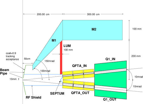
Figure 2: An illustrative diagram of the NLC intersection region, showing the positions of the last final-focus quadrupole, the exit hole for the oppposite beam, the beamstrahlung mask, and the luminosity monitor. Note that the figure is stretched by a factor of 10 in the vertical direction.

The second necessary feature is a device to calibrate luminosity and its spectrum. We have explained already that the spectrum of photon radiated from the collision region, and, concomitantly, the detailed spectrum of $e^{+}e^{-}$ center-of-mass energies, depends on the parameters of the colliding electron and positron bunches. Most physics processes at an $e^{+}e^{-}$ linear collider are not sensitive to the initial-state radiation at this level of detail, but there are a few measurements for which the knowledge of this distribution is crucial. The most important of these is the measurement of the top quark production cross section near threshold, described below in Section 4.2. Frary and Miller [44] have shown that it is possible to monitor the spectrum of $e^{+}e^{-}$ collision energies experimentally by measuring the small-angle Bhabha scattering cross section at angles near the mask. The position and size of an appropriate electromagnetic shower detector is indicated in Figure 2.

The third aspect of experimentation that deserves a special comment is the vertex detector. Because the linear collider experiments focus on the properties of the Higgs sector, which couples most strongly to heavy flavors, $b$-tagging is an important tool in many different analyses. The quality of $b$-tagging assumed in the physics studies reviewed below is that of current $e^{+}e^{-}$ detectors. However, because of the extremely small beam spot sizes expected for linear colliders, one might imagine that vertex detectors could be placed much closer to the interaction point. A recent design envisions a compact tracking system with a 4-Tesla magnetic field to sweep away soft $e^{+}e^{-}$ pairs from the bunch collision; this allows a CCD vertex detector to be placed within 2 cm of the interaction point [33].

The final noteworthy aspect of linear-collider experimentation is the availability of polarized electron beams. At low energies, where physics is dominated by the parity-conserving strong and electromagnetic interactions, the use of beam polarization has limited importance. However, for energies at the weak scale and above, the dependence on beam polarization becomes an essential part of the phenomenology. We have already noted, in Section 1.1, that at high energies the left- and right-handed electrons are distinct species with different $SU(2)\times U(1)$ quantum numbers. These species have completely different couplings both to new particles and to the gauge bosons of the standard model. Then the differences between the reactions induced by left- and right-handed electrons can be a key diagnostic tool. At the very least, one has the profound effect that the cross section for $e^{+}e^{-}\to W^{+}W^{-}$ is smaller by a factor 30 for right-handed electrons, so that the control of polarization gives one direct control of this important background process.

There are many obstacles to achieving polarized beams in circular colliders [45]. But in a linear collider, a beam that is initially polarized longitudinally naturally retains its longitudinal polarization during acceleration and transport. The degree of polarization to be expected, then, is essentially given by the properties of the electron source. For many years, the best cathode materials allowed an electron polarization of 50% in the ideal case and roughly 20 % in practice. In 1991, however, groups at SLAC and Nagoya [46, 47] learned to grow gallium arsenide cathodes as a surface layer on a substrate (e.g., GaAsP) of a slightly different lattice spacing. The resulting strain breaks the symmetry between electron levels with opposite spin and produces a material that could, in principle, give 100% electron polarization. Cathodes using this technique which are now operating in the Stanford Linear Accelerator produce a beam polarizations of about 80% at the source. Many of the studies we will review have anticipated further improvements and have assumed a beam polarization of 90–95%. It is much more difficult to produce an intense polarized positron beam [48]. Fortunately, though, this is not necessary for most experiments, since in high-energy gauge interactions, the polarized electron annihilates only on its oppositely polarized antiparticle.

2.4 $e^{-}e^{-}$, $\gamma\gamma$, and $e\gamma$ Colliders

With only small modifications, an accelerator and detector designed for high-energy $e^{+}e^{-}$ collisions can also study collisions of several other types. Since electrons and positrons can be accelerated by the same linear accelerator, it requires only a modification of the final-focus magnets to create $e^{-}e^{-}$ collisions. With some more exotic hardware in the collision region, an $e^{-}e^{-}$ collider can be converted to an $e\gamma$ or $\gamma\gamma$ collider.

An $e^{-}e^{-}$ collider would seem to lose the fundamental advantage of $e^{+}e^{-}$ colliders that the initial particles can annihilate with their full energy into a channel with vacuum quantum numbers. Nevertheless, there are a few interesting models in which exotic particles are exchanged in the $t$-channel. We will discuss such processes in supersymmetric models in Section 6.3 and in models of the strongly interacting Higgs sector in Section 7.2. From the technological point of view, the conversion of an $e^{+}e^{-}$ collider to $e^{-}e^{-}$ operation is expected to be straightforward [49]. With flat beams, the particle-antiparticle attraction does not make a large contribution to the luminosity of an $e^{+}e^{-}$ collider; an $e^{-}e^{-}$ collider with the same focusing should have a luminosity not more than a factor 3 lower.

An $e^{+}e^{-}$ collider always has some luminosity for photon-photon collisions using the Weizsäcker–Williams virtual photon field of the electron. However, it is possible to achieve a much more effective photon beam in a conceptually simple way [50]. Consider the result of shining an eV-energy laser on the high-energy electron beam, just after the last focusing magnet. Some fraction of the photons will be backscattered and achieve energies of the order of the original electron energy. These photons, now at high energy, will follow the electron trajectories ballistically and thus produce a beam spot of the same size as would have been produced by the electrons. Thus, if it is possible to achieve a one-to-one conversion of high-energy electrons to high-energy photons, the resulting collider should have the same luminosity and almost the same energy as the original $e^{+}e^{-}$ or $e^{-}e^{-}$ collider.

To make these observations quantitative, we must consider the kinematics of the electron-photon collision in more detail. We introduce a parameter $x$ that is related to the center of mass energy of the electron-photon collision by

$$x={s\over m_{e}^{2}}={4E\omega\over m_{e}^{2}}\ ,$$ (6)

where $E$ is the beam energy and $\omega$ is the photon energy. It is advantageous to make the collisions as relativistic as possible. However, it is easy to check that, when $x$ exceeds the criterion [51]

$$x_{c}=2+2\sqrt{2}\approx 4.8\ ,$$ (7)

the backscattered photons can annihilate on incoming laser photons to produce $e^{+}e^{-}$ pairs. Thus, the value given in Eq. 7 is the preferred operating point. It corresponds to a laser wavelength of 1$\mu$ at 500 GeV $e^{+}e^{-}$ center of mass energy. For fixed $x$, the maximum backscattered photon energy is $x/(1+x)\cdot E=0.83E$ when $x=x_{c}$. The photon spectrum is quite hard, and it can be made to peak at the cutoff energy by a correct choice of polarizations. For longitudinally polarized laser photons and beam electrons, the distribution in $y=E_{\gamma}/E$ has the shape

$${dn\over dy}\sim{1\over 1-y}+1-y-4r(1-r)+\Lambda rx(1-2r)(2-y)\ ,$$ (8)

where $r=y/x(1-y)$ and $\Lambda=+1$ when the electrons and the photons have both positive or both negative helicity while $\Lambda=-1$ in the opposite case. For the NLC design, the electron beam is totally converted to a high-energy photon beam with this spectrum for laser pulses of about 1 joule/pulse, compressed to a picosecond. A laser meeting this specification with a repetition rate of 1/sec is now operating in the SLAC experiment E-144 [52]; a repetition rate of 180/sec (from one or several lasers) would be required to match the NLC design.

For some physics studies, the scattered electrons, which are are at lower energy but still comoving with the high-energy photons, lead to important backgrounds and must be swept away from the photon-photon collision point by a magnetic field. We will see an example of this in Section 5.4. The constraint that this imposes on the collision region geometry is discussed in [53].

The $\gamma\gamma$ channel has the same property as $e^{+}e^{-}$ that the two colliding particles can annihilate into a state with vacuum quantum numbers. In the $\gamma\gamma$ reaction, however, processes with $t$-channel exchanges of light particles can be important, and so there is typically more background from familiar light particle pair production. Nevertheless, we will see several examples in which the $\gamma\gamma$ option contributes new information beyond that available from $e^{+}e^{-}$ annihilation.

3 $W$ BOSON PHYSICS

The process $e^{+}e^{-}\to W^{+}W^{-}$ is the largest single component of $e^{+}e^{-}$ annihilation into particle pairs at energies well above 200 GeV. The picture of the $W$ boson as a gauge boson predicts the $W$ couplings precisely from known parameters of the weak-interaction theory. Since very little of this picture is tested experimentally, one might hope to find surprises if it is probed in detail. We will show that the linear collider experiments make this possible. At the same time, the study of the $W$-boson properties provides an illustrative example of the analysis techniques that the $e^{+}e^{-}$ environment makes available.

3.1 $W$ Pair Production and Helicity Analysis

To begin, let us review the general properties of the reaction $e^{+}e^{-}\to W^{+}W^{-}$ within the standard model [54]. The reaction proceeds via the Feynman diagrams shown in Figure 3. From the second of these diagrams, it is clear that the process has a strong forward peak associated with $t$-channel neutrino exchange. The presence of this peak is correlated with polarization; it occurs, quite specifically, in the reaction $e^{-}_{L}e^{+}_{R}\to W^{-}_{L}W^{+}_{R}$.

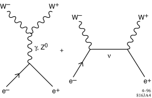
Figure 3: Feynman diagrams for $e^{+}e^{-}\to W^{+}W^{-}$.

For the pair production of longitudinally polarized $W$ bosons, there is a different and more interesting story. The diagrams of Figure 3 individually violate unitarity. It is a wonderful property of the standard model that the sum of the diagrams, adding the $\gamma$ and $Z^{0}$ exchanges coherently, contains the correct cancellations to preserve unitarity. In fact, at high energy, the cross section for pair-production of longitudinal $W$ bosons takes the simple form

$${d\sigma\over d\cos\Theta}={\pi\alpha^{2}\over 128s}\biggl{(}{1+4\sin^{4}\theta_{w}\over\cos^{4}\theta_{w}\sin^{4}\theta_{w}}\biggr{)}\sin^{2}\Theta\ ,$$ (9)

where $\Theta$ is the production angle in the center-of-mass system. These facts are explained in the standard model by the statement that the $W$ obtains a longitudinal component only by virtue of the Higgs mechanism. The gauge symmetry associated with the $W$ is spontaneously broken, a Goldstone boson is created, and this boson becomes the extra, longitudinal polarization state of the massive $W$. The longitudinal part of the $W$ then inherits the properties of the eaten scalar boson, such as the $\sin^{2}\Theta$ production cross section shown in Eq. 9. This phenomenon, that a longitudinal gauge boson acquires at high energy the properties of a Goldstone boson, is in fact a general result, called the Goldstone Boson Equivalence Theorem [55, 56, 57, 58].

Figure 4: Angular distributions for $W$ bosons of various helicity in $e_{L}^{-}e_{R}^{+}\to W^{+}W^{-}$. The differential cross sections are given in units of R at $E_{\hbox{\scriptsize CM}}=1$ TeV.

Combining these two pieces of physics, we are led to expect a complex pattern for the cross sections for $e^{+}e^{-}$ annihilation to $W$ pairs of various helicity. For an initial $e^{-}_{L}$, the predictions of the standard model at a center-of-mass energy of 1 TeV are shown in Figure 4. For an initial $e^{-}_{R}$, the cross section is dominantly longitudinal $W$ pair production, with a rate 1/5 of the longitudinal pair production cross section shown in the figure.

Can we test the composition of this complex mixture of $W$ boson states experimentally? This is quite straightforward in the experimental environment of linear colliders. By reconstructing events with $W$ pair production and decay, we will obtain not only information on the distribution in the production angle $\Theta$ but also information on the individual $W$-boson decay angles. Since the decay angular distribution encodes the $W$ polarization, the distributions for $W$ pair production can be determined for each final-state $W$ polarization.

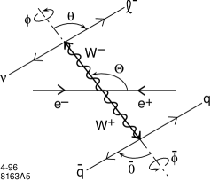
Figure 5: Production and decay angles in $e^{+}e^{-}\to W^{+}W^{-}$.

To understand how the analysis is done, consider, for simplicity, the case in which one of the $W$’s decays hadronically and the other $W$ decays leptonically to $e$ or $\mu$. (This sample includes 30% of all $W$ pair events.) The missing neutrino can be reconstructed, even allowing for initial-state radiation, and so the whole event is determined. The event is characterized by the production angle $\Theta$ and decay angles $\theta$, $\phi$ on each side, as shown in Figure 5. The angle $\theta$ is related to the $W^{-}$ helicity $h_{W}$ through the decay distributions

$${d\Gamma/d\cos\theta}\sim\cases{(1+\cos\theta)^{2}&$h_{W}=-1$\cr 2\sin^{2}\theta&$h_{W}=0$\cr(1-\cos\theta)^{2}&$h_{W}=+1$\cr}\ ,$$ (10)

and just oppositely for $W^{+}$. A nontrivial dependence on $\phi$ appears due to interference between the possible $W$ polarizations. There is an observational ambiguity on the hadronic side, since it is not clear which of the two observed jets originates from the quark and which from the antiquark. Nevertheless, each event can be plotted in a 5-dimensional space of observables $(\Theta,\theta_{W^{+}},\phi_{W^{+}},\theta_{W^{-}},\phi_{W^{-}})$, and it is possible to compare to theoretical distributions over this set of five variables.

Several simulation studies of this kinematic fitting have been performed [36, 68, 69]. As an example, consider the analysis of [36]. Events with the topology of a lepton and two jets are selected such that the calorimetrically determined hadronic invariant mass is consistent with the mass of the $W$, the missing energy is consistent with being a single massless particle, and the sum of this momentum vector with that of the lepton gives the $W$ mass to within 20 GeV. This yields an event sample of 98% purity, into which $W$ events of the required topology are selected with 36% efficiency. Kinematic fitting produces the distributions shown in Figure 6 for the $WW$ center of mass energy $\sqrt{\hat{s}}$, $\cos\Theta$, and the leptonic side $W$ decay angles $\theta$ and $\phi$. These results give a firm foundation for the detailed study of $W$ pair production, and for more exotic reactions which have $W$ pair production as a standard-model background.

3.2 Anomalous Couplings of the $W$

Before going on to more complex reactions, it is worth asking what can be learned from the detailed study of $e^{+}e^{-}\to W^{+}W^{-}$. To make a precise statement, we will introduce a conventional parametrization of the $WW\gamma$ and $WWZ$ couplings, and discuss the expected size of the parameters indicating a deviation from the standard model. Electroweak radiative corrections, which typically contribute at the level of a few percent, must also be taken into account [59].

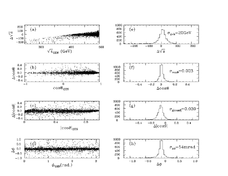
Figure 6: Reconstruction of production and decay angles in $e^{+}e^{-}\to W^{+}W^{-}$, from [36].

For historical reasons, most studies of the $W$ boson couplings assume a general vertex functions of the following form [54]:

$${\cal L}_{WWV} = ig_{V}\bigl{(}g_{1V}(W^{\dagger}_{\mu\nu}W^{\mu}V^{\nu}-W^{\dagger}_{\mu}V_{\nu}W^{\mu\nu})$$ (11)

$$+\kappa_{V}W^{\dagger}_{\mu}W_{\nu}V^{\mu\nu}+\lambda_{V}{1\over m_{W}^{2}}W^{\dagger}_{\lambda\mu}W^{\mu}{}_{\nu}V^{\nu\lambda}\bigr{)}\ ,$$

where $V$ is $\gamma$ or $Z$, $g_{\gamma}=e$, $g_{Z}=e\cos\theta_{w}/\sin\theta_{w}$, $W_{\mu}$ is the $W^{-}$ field, $W_{\mu\nu}=\partial_{\mu}W_{\nu}-\partial_{\nu}W_{\mu}$, and $V_{\mu\nu}=\partial_{\mu}V_{\nu}-\partial_{\nu}V_{\mu}$. In the standard model at tree level, $g_{1V}=1$, $\kappa_{V}=1$, $\lambda_{V}=0$ for both $\gamma$ and $Z$. It is convenient to define $\Delta\kappa_{V}=(\kappa_{V}-1)$. The expression given in Eq. 11 omits possible $CP$-violating couplings and also, perhaps with not so strong motivation, couplings that violate $C$ and $P$ separately in the gauge boson sector. (For consideration of these latter couplings, see [60].) If we ignore possible $q^{2}$-dependence of the $W$ form factors, as is done in Eq. 11, $g_{\gamma}=e$ expresses the electric charge of the $W$ boson. The parameters $\Delta\kappa_{\gamma}$ and $\lambda_{\gamma}$ are then related to the magnetic dipole moment and the electric quadrupole moment of the $W$:

$$\mu_{W}={e\over 2m_{W}}(2+\Delta\kappa_{\gamma}+\lambda_{\gamma})\ ,\qquad Q_{W}=-{e\over m_{W}^{2}}(1+\Delta\kappa_{\gamma}-\lambda_{\gamma})\ .$$ (12)

Often, $g_{1Z}$ is also taken to have its standard-model value, leaving still a problem of four unknown parameters to be constrained experimentally.

Should we expect substantial deviations from the standard model in the values of $\kappa_{V}$ and $\lambda_{V}$? In the older literature, this question is framed as the question of whether the $W$ bosons are actually the gauge bosons of a non-Abelian gauge theory. If there is room to assume that the $W$ couplings are not necessarily those of Yang-Mills theory, any constraints on $\kappa_{V}$ and $\lambda_{V}$ should be interesting. However, in this general context, it is difficult to understand why loop diagrams involving $W$ bosons, which play an important role in the electroweak radiative corrections tested at LEP and SLC, apparently agree well with the predictions of the standard model.

Over the past few years, a more conservative point of view has evolved in which the interactions of $W$ bosons are parametrized by gauge-invariant interactions of the $W$ fields with the electroweak symmetry breaking sector [61, 62, 63, 64]. Consider, for example, the effect of coupling the $W$ boson field to a nonlinear-sigma-model field $U$ whose expectation value $\left\langle{U}\right\rangle=1$ signals $SU(2)\times U(1)$ breaking. The coupling with two derivatives reproduces the conventional $W$ mass term when $U$ is replaced by its vacuum expectation value, but allowing couplings with four derivatives brings in the more general terms [61, 65]:

$$\Delta{\cal L} = -iL_{9}\mbox{Tr}(g^{\prime}B_{\mu\nu}D^{\mu}UD^{\nu}U^{\dagger}+gW_{\mu\nu}D^{\mu}U^{\dagger}D^{\nu}U)$$ (13)

$$+L_{10}gg^{\prime}\mbox{Tr}(U^{\dagger}B_{\mu\nu}UW^{\mu\nu}),$$

where $g$, $g^{\prime}$ are the $SU(2)\times U(1)$ couplings, and $D_{\mu}U=(\partial_{\mu}-igUW_{\mu}+ig^{\prime}B_{\mu}U$). From Eq. 13, one obtains a special case of the vertex written in Eq. 11, with $\lambda_{V}=0$ and

$$\kappa_{\gamma} = 1-g^{2}(L_{9}+L_{10})$$

$$\kappa_{Z} = 1-{1\over 2}(g^{2}-g^{\prime}{}^{2})L_{9}+2e^{2}L_{10}/(c_{w}^{2}-s_{w}^{2})$$

$$g_{1Z} = 1-{1\over 2}g^{2}L_{9}/c_{w}^{2}+g^{\prime}{}^{2}L_{10}/(c^{2}_{w}-s^{2}_{w})\ ,$$ (14)

where $s_{w}=\sin\theta_{w}$, $c_{w}=\cos\theta_{w}$.

This point of view, however, suggests rather different values for the expected anomalies. A typical model leading to anomalous $W$ interactions would be one in which the electroweak symmetry breaking sector contained new strong interactions at TeV energies. In such a model, the new strongly interacting particles would give virtual corrections to the $W$ couplings. A reasonable way to estimate this effect would be to set the dimensionless parameters $L_{9}$, $L_{10}$ in Eq. 13 equal to the values of the corresponding parameters in the nonlinear-sigma-model description of QCD [66]. This gives: $L_{9}\sim L_{10}\sim 0.045$, or $\Delta\kappa\sim 10^{-2}$. It is worth noting that $L_{10}$ is related to the $S$ parameter [67] of precision electroweak physics through $S=-L_{10}/\pi$, and that the current constraint on $S$ limits the contributions to the anomalous couplings from $L_{9}$ to be of order $10^{-3}$.

Can linear collider experiments meet this extremely challenging criterion for the appearance of deviations in the $W$ interactions? Remarkably, they can. There are two aspects of the physics that improve the sensitivity. The first is common to all determinations of the $W$ couplings at high energy: because anomalous additions to the $W$ couplings do not respect the gauge cancellations (or, in the language of Eq. 13, because they multiply higher-dimension operators), these coefficients multiply terms in the cross section formulae which grow as $(s/m_{W}^{2})$ relative to the leading-order terms. The second is peculiar to the $e^{+}e^{-}$ environment: the full-event analysis described in the previous section brings the $W$ polarization information into the analysis as a powerful constraint.

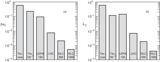
Figure 7: Comparison of limits on anomalous $W$ couplings from different colliders, from ref. [71].

The most detailed study of the determination of $W$ couplings at linear colliders has been done by Barklow and is described in [68, 70]. His analysis followed the general strategy described in the previous section. Barklow assumes for simplicity the very precise tracking resolution of the JLC detector; under this assumption, errors in lepton and jet reconstruction are negligible compared to the statistical errors. Reconstructed $W$ events obtained from the scheme of cuts described above are fitted to distributions parametrized by $\Delta\kappa_{V}$, $\lambda_{V}$. In Figure 7, taken from ref. [71], the expected sensitivity of the linear collider experiments is compared to the estimated sensitivity of other anticipated experiments. The analyses shown in this figure consistently assume a particular two-parameter formula which relates the $\gamma$ and $Z$ anomalous couplings [72]; thus, it may be somewhat optimistic for all colliders shown.

In comparing the sensitivity of experiments at hadron and lepton colliders to the anomalous W couplings, it is important to note that hadron experiments produce $W$ pairs with a wide range of values of the $WW$ invariant mass $\hat{s}$. Because the anomalous coupling multiply terms which in the amplitude grow as $(\hat{s}/m_{W}^{2})$, the greatest sensitivity to anomalous couplings comes at the highest values of $\hat{s}$. However, at some point these enhancements must be cut off by form factors depending on $\hat{s}$, and the results depend on assumptions about these form factors. At $e^{+}e^{-}$ colliders, the center of mass energy is fixed and there is no corresponding ambiguity.

An alternative window into $W$ couplings is provided by the reactions $e\gamma\to W\nu$ [73, 76] and $\gamma\gamma\to W^{+}W^{-}$ [74, 75]. These reactions can be studied at a linear collider for which Compton backscattering has been used to create a photon beam, as described in Section 2.4. For the $\gamma\gamma$ reaction, complete events can be reconstructed using the same technique that we described for $e^{+}e^{-}\to W^{+}W^{-}$. The sensitivity of this reaction to anomalous couplings is smaller, because the cross section for producing transversely polarized $W$ pairs, which is less sensitive to the new interactions, is more predominant. Nevertheless, these experiments are expected to give independent limits on the parameters $\kappa_{\gamma}$, $\lambda_{\gamma}$ at the 1% level [36]. The $\gamma\gamma$ reaction can also be sensitive to a possible $WW\gamma\gamma$ 4-boson anomalous vertex [77].

4 TOP-QUARK PHYSICS

Beyond the $W$ and $Z$, there is one more heavy particle of the standard model, the top quark. The reaction $e^{+}e^{-}\to t\overline{t}$ has a cross section of about 2.0 units of R asymptotically, and this value is reached rapidly as one crosses the threshold energy of $2m_{t}$.

Using an analysis in the same spirit as that described above for the $W$ boson, it is possible at a linear collider to make a precision study of the top quark couplings to $\gamma$, $Z$, and $W$. But, in addition, there are interesting physics issues associated with the $t\overline{t}$ threshold region. For lighter quarks, the energy region just below the threshold contains the quarkonium states. For the top quark, this quarkonium region is replaced by a region of about 10 GeV in width in which the physics is controlled by the competition between $t\overline{t}$ binding and decay. The linear collider will be the first accelerator with sufficient resolution in $t\overline{t}$ center of mass energy to make a detailed study of this region.

4.1 Properties of the Heavy Top Quark

The top quark is so much heavier than the other quarks that much of the intuition of ordinary hadronic physics is simply invalid when applied to $t\overline{t}$ systems. To discuss the program of experimental measurements on the top quark, we must first review the general properties that are expected for this particle in the standard model.

The crucial difference between the top quark and all lighter quarks is that the top quark is sufficiently massive to decay to an on-shell $W$ boson. This means that the top quark is not a “stable particle,” but rather decays in a time short compared to typical hadronic scales. The expression for the top-quark decay width as a function of its mass, in the limit $m_{b}=0$, is

$$\Gamma(t\to bW) = {\alpha_{w}\over 16}{m_{t}^{3}\over m_{W}^{2}}\left(1-{m_{W}^{2}\over m_{t}^{2}}\right)^{2}\left(1+2{m_{W}^{2}\over m_{t}^{2}}\right)\left(1-2.9{\alpha_{s}\over\pi}\right)$$ (15)

$$\sim (1.4\ \hbox{\rm GeV})\left({m_{t}\over 175\ \hbox{\rm GeV}}\right)^{3}\ .$$

The QCD correction [78] is evaluated at $m_{t}=175$ GeV; the full theory of the top quark width is reviewed in [79]. The large size of the top-quark width is insured by the unexpected $m_{t}^{3}$ growth of the formula given in Eq. 15. This dependence is due to the enhanced coupling of the top quark to the longitudinal polarization state of the $W$ boson. Just as in $e^{+}e^{-}\to W^{+}W^{-}$, the couplings of this state reflect the fact that it originates as a Higgs boson; the Higgs particle couples more strongly than a transversely polarized $W$ to the heavy quark.

The large width of the top quark has striking implications [80, 81, 82]. Because the top quark decays before nonperturbative strong-interaction processes have time to act, the top quark is completely a creature of perturbative QCD. In production and decay processes, the top quark retains its identity and its spin orientation. In the vicinity of the $t\overline{t}$ threshold, the spectrum of top-antitop states is determined by the gluon-exchange potential without a need to invoke phenomenological confining interactions [83] (though the large width is an essential complication). Quantitatively, the width of the top quark takes it off the mass shell by an amount

$$Q\sim\sqrt{m_{t}\Gamma_{t}}\sim 15\ \hbox{\rm GeV}\ ;$$ (16)

thus all strong-interaction processes involving top are computable in perturbation theory using $\alpha_{s}$(15 GeV) $\sim 0.16$.

4.2 The $t\overline{t}$ Threshold in $e^{+}e^{-}$ Annihilation

We begin our more specific discussion of top physics at the $t\overline{t}$ threshold. The general properties of the $t\overline{t}$ threshold are made clear by the following physical picture: the $t\overline{t}$ pair is produced at zero separation and then the quarks move outward nonrelativistically. However, when they reach a separation of $Q^{-1}$ given in Eq. 16, they decay via $t\to Wb$. The decay rate $\Gamma$ is roughly the same as the oscillation frequency in the QCD potential, of order $(\alpha_{s}^{2}m_{t})^{-1}$. Thus, the QCD potential plays an important role in the physics of the threshold region, but the top and antitop live for so short a time that no discrete bound states can form. Also, on this short time scale, the nonperturbative confining interaction is irrelevant.

This picture of the $t\overline{t}$ threshold was made quantitative in a series of papers by Fadin and Khoze [83]. These authors argued that the total cross section for $t\overline{t}$ production could be written as a sum over eigenfunctions of the nonrelativistic Schrödinger equation for the QCD potential,

$$\sigma(e^{+}e^{-}\to t\overline{t})={8\pi^{2}\alpha^{2}\over 3m_{t}^{4}}\mbox{Im}\sum_{n}{\psi^{*}_{n}(0)\psi_{n}(0)\over E_{n}-E_{\hbox{\scriptsize CM}}+i\Gamma_{t}}\ ,$$ (17)

or more generally, in terms of the Green’s function for this potential problem. The Green’s function is evaluated at an off-shell energy, shifted by $i\Gamma_{t}$ because both the $t$ and $\overline{t}$ are unstable. The consequences of this formula were worked out for realistic QCD potentials, and including next-to-leading order QCD corrections and the smearing due to initial-state radiation, in [84, 85]. For values of $m_{t}$ below 120 GeV, the 1S quarkonium resonance is still clearly apparent as a peak in the cross section. However, as the top mass is increased, this state fades out as a distinct spectral feature. Naively, it seems that the disappearance of the resonances in the spectrum of toponium is an unwanted consequence of the large top mass. But precisely the reverse is true: as the top-quark mass increases, the threshold shape is more precisely determined by perturbative physics and therefore is a more incisive probe of the fundamental top-quark properties.

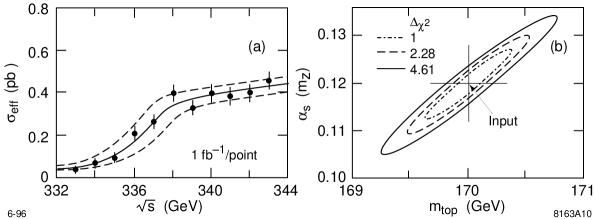
Figure 8: Measurement of the top quark mass from the threshold shape, from the simulation results of [88] with 11 fb^-1 of data, assuming a 170-GeV top-quark mass. The solid curve gives the theoretical expression for the $t\overline{t}$ threshold, for $\alpha_{s}(m_{Z})=0.12$, including initial-state radiation, beamstrahlung, and a 0.1% energy spread from the accelerator. The dashed curves show the theoretical predictions for $\alpha_{s}(m_{Z})=0.11$ and 0.13, from bottom to top.

Even including the effect of the top-quark width, the cross section rises rapidly at the threshold, and so it is straightforward to obtain a very accurate value of the top quark mass. Simulation studies of the measurement of the $t\overline{t}$ production cross section near threshold have been carried out by several groups [86, 87, 88, 89]. These analyses include a realistic selection of $t\overline{t}$ events. For example, the analysis of [88] selects $t\overline{t}\to 6$ jet events through the following set of cuts: First choose events with visible energy greater than 200 GeV and total $p_{T}$ less than 50 GeV. Then cluster the tracks into 6 jets. Select events with two 2-jet pairs consistent with $m_{W}$ and such that adding another jet gives a mass consistent with $m_{t}$, within loose cuts. Finally, impose a thrust cut, $T<0.75$. This procedure selects hadronic $t\overline{t}$ events with 63% efficiency. The final cut reduces the dominant background from $W^{+}W^{-}$ production to less than 10% of the top quark signal, and of course this background has no threshold. Under these conditions, a luminosity of 10 fb^-1 scattered over the threshold region, as shown in Figure 8, still suffices to determine $m_{t}$ to an accuracy of 300 MeV. This measurement also determine the strength of the QCD potential, which can be parametrized by the strong coupling constant $\alpha_{s}$ (for example, by the value of $\alpha_{s}(m_{Z})$ in the $\overline{\hbox{\rm MS}}$ scheme for QCD calculations). The determinations of $m_{t}$ and $\alpha_{s}$ are correlated; if $\alpha_{s}$ is known from other measurements to $0.002$ (half the present uncertainty), the error on $m_{t}$ decreases to 200 MeV. This should be contrasted with projected determinations of the top quark mass in hadronic collisions, which are limited to an accuracy of about 2 GeV [90].

For such accurate values of $m_{t}$, it is important to clarify the precise meaning of the measurement [91]. The value of $m_{t}$ which enters the top quark threshold calculations is the ‘pole mass’, the mass appropriate to treating the top quark as an on-shell state of perturbative QCD. A more interesting quantity is the mass of the top quark defined according to the $\overline{\hbox{\rm MS}}$ scheme, which can be directly related to the underlying values of the short distance couplings which are responsible for quark masses. These quantities are related by

$$(m_{t})_{\hbox{\scriptsize pole}} = (m_{t})_{\overline{\hbox{\scriptsize MS}}}\bigl{[}1+{4\over 3}{\alpha_{s}\over\pi}+\cdots\bigr{]}$$ (18)

$$= (m_{t})_{\overline{\hbox{\scriptsize MS}}}+(9.7\ \hbox{\rm GeV}\pm 2.1\ \hbox{\rm GeV})\ ,$$

where we have included the 2-loop contribution [92], evaluating the $\overline{\hbox{\rm MS}}$ mass at the pole mass, and we have chosen this to be 175 GeV in the numerical estimate. The error given is the magnitude of the 2-loop correction. The corrections to the $t\overline{t}$ threshold shape are understood at the next-to-leading order in $\alpha_{s}$ [93], but subtle questions remain about the size of the corrections of order $\alpha_{s}^{2}$, in particular, the effects due to the decrease in the width of a top quark at off-shell, spacelike momenta [94, 95, 96].

The study of the $t\overline{t}$ threshold allows an accurate measurement of the top-quark width. This can be done, first, by measuring the threshold shape, which is determined by this width in the way that we have just described. From a fit to the threshold shape with a 10 fb^-1 data sample, one obtains a 20% measurement of the top-quark width. But there are two additional techniques available. The first involves the momentum distribution of the decaying top and antitop. The reconstruction of the top-quark kinematics which is implicit in the cuts defined above allows one to determine this distribution directly. Thus, one obtains a snapshot of the top-quark wavefunction, in momentum space, at the given center of mass energy. This wavefunction is a linear combination of contributions from nearby $t\overline{t}$ states; it contains an increased admixture of distant states, with higher momentum components, if the top-quark width is large. The theory of this momentum distribution is worked out in detail in [94, 97]. The second of these probes is the forward-backward asymmetry of the $t\overline{t}$ system [98]. Though the nonrelativistic $t\overline{t}$ system is dominantly produced in an S-wave, the axial-vector current coupling to the $Z^{0}$ can also produce P-wave states. The interference of these components produces the asymmetry. This interference effect is sensitive to the overlap of the $t\overline{t}$ resonances, smeared by the top width, and so it also increases as the top width is increased.

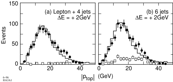
Figure 9: Reconstructed top-quark momentum distribution in the $t\overline{t}$ threshold region, giving the wavefunction of the virtual $t\overline{t}$ state, from [88]. The solid squares indicate the combinatorial background due to wrong jet assignment; backgrounds from other physics processes are negligible.

This strategy was tested in simulation studies of reconstruction of the top-quark momentum distribution [87, 88]. We will review the study [88] in some detail. In this work, top quarks were selected by a set of cuts more restrictive than those described above, imposing the criteria that 2-jet combinations sum to $m_{W}$ within 8 GeV and that 3-jet combinations sum to $m_{t}$ within 15 GeV. In addition, $b$ jets are identified by vertex tagging and required to be roughly back-to-back with the associated $W$ bosons (since the parent top quarks are moving slowly). These additional cuts reduce the efficiency to 4.9% but remove the $W^{+}W^{-}$ background and also go far toward resolving the combinatorial ambiguity in top reconstruction. A similar analysis can be applied to $t\overline{t}$ events with one lepton in the final state, and the sign of the lepton can then be used to measure the forward-backward asymmetry. The reconstruction of the top-quark momentum distribution, at an energy 2 GeV above the nominal 1S peak, is shown in Figure 9. In this analysis, which used a top-quark mass of 150 GeV, a luminosity sample of 100 fb^-1 yields the top-quark width from the momentum distribution and the forward-backward asymmetry with errors of 4% and 7%, respectively, for the two techniques.

To compare the measurement of the top-quark width that will be available from a linear collider to that expected from hadron colliders, we should differentiate two possible sources of a deviation of this quantity from the standard model. First, the top width might be larger than the standard model value due to the presence of new decay modes. The presence of such new decay modes will affect the leptonic branching ratio of the top quark, a quantity which should be measured in the Fermilab collider experiments to a few percent [90]. However, such new decay modes can be searched for directly in the $e^{+}e^{-}$ environment by examining the system recoiling against a reconstructed top quark. As examples of analyses with this general strategies, a decay of the top quark into a charged Higgs boson plus a $b$ quark with a 5% branching ratio can be identified at the 3 $\sigma$ level with 10 fb^-1 of data, and the decay into a top squark and photino with a 5% branching ratio can be identified at the 3 $\sigma$ level, for the mass values ($m_{\tilde{t}},m_{\tilde{\gamma}}$) = (100,40), with 30 fb^-1 [99]. In general, direct searches for manifestations of new decay modes are expected to be much more accurate than probes using the quark total width.

On the other hand, even if the top quark decays dominantly to $W^{+}b$, its width might be lowered if the Cabbibo-Kobayashi-Maskawa mixing angle $V_{tb}$ is not closely equal to 1, or if the $t{\overline{b}}W$ coupling is enhanced by a nontrivial form factor. There are two experiments at hadron colliders that are sensitive to the strength of the top coupling to $bW$. The first of these is the measurement of the subprocess $W^{+}g\to t\overline{b}$ [100]. However, the analysis of this experiment has substantial QCD uncertainty as well as the uncertainty of the gluon distribution. A more promising method is the measurement of $\sigma(q\overline{q}\to t\overline{b})/\sigma(q\overline{q}\to\ell\nu)$ [101]. The measurement suffers from a substantial background due to $q\overline{q}\to Wb\overline{b}$, which accounts for almost 1/3 of the events under the $t$ mass peak in the $W^{+}b$ distribution, and an additional 10% background from $t\overline{t}$ production in which some jets are not reconstructed. If these backgrounds can be subtracted without introducing a systematic error, this measurement should give a measurement of the $t{\overline{b}}W$ coupling corresponding to a 10% uncertainty in the top quark width with 12 fb^-1 of data at the Tevatron collider. The signal is masked at LHC by the high rate of $gg\to t\overline{t}$.

The comparison of these techniques nicely illustrates the relation of $e^{+}e^{-}$ and $pp$ experiments. The $pp$ environment gives a single observable which can be determined with great statistical power. But the $e^{+}e^{-}$ environment allows a variety of measurements which allow almost a pictorial view of the interactions of top quarks in their binding potential. To give another example of the use of this detailed picture, the interaction of the top quark with the Higgs boson introduces an additional positive Yukawa term into the $t\overline{t}$ potential. For a light Higgs boson with standard-model couplings, and for $m_{t}$ = 175 GeV, its strength is 15% of the strength of the QCD potential. For a known value of the Higgs mass (whose measurement we will explain in Section 5.2) the observation of an enhancement in the threshold cross section due to this effect measures the $t\overline{t}h$ coupling [85, 102, 103]. For $m_{h}$ = 100 GeV and standard-model couplings, the coupling constant can be determined to 25% accuracy with 20 fb^-1 of data [88]. In models in which the top quark has new interactions associated with electroweak symmetry breaking, this coupling can be strong, leading to significant threshold enhancements. More generally, the $t\overline{t}$ system at threshold is an ideal laboratory for the exploration of small corrections to the picture of binding provided by QCD.

4.3 Analysis of $t\overline{t}$ gauge couplings

Just as for the $W$ boson, it is interesting to ask whether the top quark has non-standard couplings to electroweak gauge bosons. This question can be addressed directly at $e^{+}e^{-}$ colliders by exploiting the naturally large forward-backward and polarization asymmetries of $t\overline{t}$ production and decay. These asymmetries reflect the very different couplings of the left- and right-handed components of the top quark to the $SU(2)$ gauge interactions and the fact already noted that the top quark retains its polarization from production to decay.

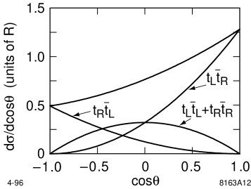
Figure 10: Angular distribution of top quarks in various polarization states from $e^{-}_{L}e^{+}\to t\overline{t}$ at $E_{\hbox{\scriptsize CM}}=400$ GeV.

Though experiments on $t\overline{t}$ couplings are best done at center-of-mass energies below 500 GeV, it is easiest to see the essential features of the phenomenology by thinking first about production at very high energy. If we consider $E_{\hbox{\scriptsize CM}}\gg m_{t},m_{Z}$, the cross section for producing top quark pairs from a left-handed electron beam is given by

$${d\sigma\over d\cos\theta}={3\pi\alpha^{2}\over 4s}\bigl{[}|f_{LL}|^{2}(1+\cos\theta)^{2}+|f_{LR}|^{2}(1-\cos\theta)^{2}\bigr{]}$$ (19)

where, with $I^{3}_{H}={1\over 2},0$ for $H=L,R$,

$$|f_{LH}|^{2} = \left|-{2\over 3}-{({1\over 2}-\sin^{2}\theta_{w})(I^{3}_{H}-{2\over 3}\sin^{2}\theta_{w})\over\sin^{2}\theta_{w}\cos^{2}\theta_{w}}\right|^{2}$$ (20)

$$= \cases{1.4&$e^{-}_{L}e^{+}_{R}\to t_{L}\overline{t}_{R}$\cr 0.2&$e^{-}_{L}e^{+}_{R}\to t_{R}\overline{t}_{L}$\cr}$$

That is, a left-handed electron beam dominantly produces forward-moving, left-handed top quarks. The angular distribution for more realistic conditions, $E_{\hbox{\scriptsize CM}}=500$ GeV and $m_{t}=175$ GeV, is shown in Figure 10. A third component, $(t_{L}\overline{t}_{L}+t_{R}\overline{t}_{R})$, is present with a cross section proportional to $(m_{t}/E_{\hbox{\scriptsize CM}})^{2}$. A right-handed electron beam gives a somewhat larger asymmetry between the two top helicities, and a total cross section lower by a factor of 2.

The spin of the top quark can be measured through its decay angular distribution. Returning to Equation 15 and including the dependence on the angle $\theta$ between the $W$ direction and the top spin, one finds that the factor $(1+2m_{W}^{2}/m_{t}^{2})$ expands to

$${d\Gamma\over d\theta}\sim\left[(1+\cos\theta)+2{m_{W}^{2}\over m_{t}^{2}}(1-\cos\theta)\right]$$ (21)

where the first term represents the decay to a longitudinally polarized $W$ and the second term to a left-handed $W$. Alternatively, if the $W$ is observed to decay leptonically, the distribution of the angle $\chi$ between the lepton direction and the top spin is $(1+\cos\chi)$.

The QCD radiative corrections to the production [104] and decay [105] distributions have been computed and turn out to be quite small. Formulae describing the spin correlations in the final decay products from $e^{+}e^{-}\to t\overline{t}$ have been presented at the tree level in [106], and at the one-loop level in [107, 108]. The paper [108] is especially explicit and also describes an implementation of these formulae as a parton-level Monte Carlo program.

To discuss the constraints that can be obtained, we must parametrize the top quark couplings to gauge bosons. In general, we can write a gauge boson coupling to the top quark in the form [109]

$${\cal L}=g_{ttV}\bigl{[}F_{1L}\overline{t}\gamma^{\mu}t_{L}V_{\mu}+F_{2L}{1\over 2m_{t}}\overline{t}\sigma^{\mu\nu}t_{L}V_{\mu\nu}+(L\to R)\bigr{]}\ ,$$ (22)

where $V$ is $\gamma$ or $Z$ and $V_{\mu\nu}=\partial_{\mu}V_{\nu}-\partial_{\nu}V_{\mu}$. For $W$, replace $t_{L}$ by $b_{L}$. This equation defines chiral form factors $F^{V}_{1L,R}$, $F^{V}_{2L,R}$. Conservation of CP requires $F_{2L}=F_{2R}$ for $V=\gamma,Z$. There is a substantial literature on the experimental manifestations of CP violation in the top form factors [110, 111, 112]; however, in realistic models, these effects are typically at the $10^{-3}$ level at most, and the linear collider would not be expected to provide sufficient statistics to see the effect (see, however, [113]).

The sensitivity of linear collider experiments to deviations from the standard-model values of the $F^{V}_{i}$ has been investigated by several groups using parton-level simulations and a full-event analysis similar to that described in Section 3.1 for $W$ pair production [110, 114, 115]. The results of these simulations may be summarized by the statement that 10% variations of the $F^{V}_{i}$ in arbitrary combinations can be recognized or excluded at the 95% confidence level using luminosity samples of 100 fb^-1, making this a feasible project for the first-stage of the NLC. The comparison of this level of sensitivity to the predictions of models will be discussed in Section 7.5.

The form factors in the top-quark decay amplitude can also be studied at threshold, and with higher statistics, by using the fact that, in pair production of nonrelativistic fermions, the spin in the final state follows the spin of the initial electron. The theory of the top-quark polarization near threshold, taking into account the details of the $b\overline{t}$ binding, is presented in [117]. Alternatively, this study can be done by noting that, in production above threshold, the top-quark spin is still strongly aligned with the electron spin direction as measured in the top rest frame [118].

5 THE HIGGS SECTOR (WEAK COUPLING)

Up to this point, we have discussed tests of the standard model in the pair-production of $W$ bosons and top quarks. We have emphasized that these standard-model processes have interesting qualitative features and provide many experimental handles in the search for anomalies. These features add to the general promise of the $e^{+}e^{-}$ environment for new particle searches.

However, in presenting the motivation for a new accelerator, one must also ask how the window that it provides corresponds to general expectations for where new physics can be found. This necessarily brings us into the detailed study of theoretical models. For the reasons presented in Section 1.1, we will concentrate here on models of electroweak symmetry breaking. In Sections 5-7, we will review the most important models of this phenomenon, explaining, for each class of models, the relevance of linear-collider experiments.

5.1 Higgs Bosons at $e^{+}e^{-}$ Colliders

If the electroweak symmetry breaking occurs in a weakly-coupled theory, the symmetry breaking must arise from the vacuum expectation values of elementary scalar fields. In general, three components of the scalar fields combine with the $W^{\pm}$ and $Z^{0}$ to form the longitudinal components of these vector bosons, while the remaining scalar fields are massive scalar particles. In models of this type, these particles, called Higgs bosons, are the direct manifestations of the symmetry-breaking mechanism and therefore deserve intensive study.

In the minimal standard model, the theory contains one multiplet of scalar fields with four degrees of freedom. After symmetry breaking, one neutral scalar Higgs boson is left over. In more complex models, there may be additional multiplets of scalar fields; then the spectrum of physical Higgs bosons will also be more interesting. For example, supersymmetric models require at least two scalar-field multiplets. Then one finds five physical Higgs fields—two neutral scalars $h^{0}$ and $H^{0}$, a neutral pseudoscalar $A^{0}$, and charged scalars $H^{\pm}$. In general, these particles are linear combinations of components of the original two Higgs fields $\phi_{1}$ and $\phi_{2}$. One mixing angle in particular, the angle $\beta$ defined by

$$\tan\beta=\left\langle{\phi_{2}}\right\rangle/\left\langle{\phi_{1}}\right\rangle\ ,$$ (23)

appears as a parameter in many phenomenological relations.

The mass of the Higgs boson of the minimal standard model is not predicted by the theory. This mass is constrained by direct searches at LEP to be above 65 GeV [119], and it is constrained to be below roughly 700 GeV by the consistency requirements for nonlinear scalar field theories [120]. The lower end of the spectrum corresponds to a scalar field with weak self-interactions—$m_{h}$ is of order $m_{Z}$ when the Higgs self-coupling is of the order of the weak-interaction coupling constant—and the high end corresponds to a field with strong self-interactions. It requires a model that can explain the electroweak symmetry breaking with specific weak or strong coupling dynamics to predict the Higgs-boson mass. In such models, one typically finds values at the low or high extremes of this range.

Supersymmetric models, for example, favor Higgs-boson masses at the low end of the allowed range. In the case of two Higgs multiplets and no additional $SU(2)$-singlet fields—the conditions that define the ‘Minimal Supersymmetric Standard Model’ (MSSM)—these models predict that the lightest scalar $h^{0}$ has a mass below 130 GeV [121, 122, 123]. This bound is relaxed in models that contain additional fields. However, these models also restrict the Higgs boson masses from a more general principle. Supersymmetric models are consistent with the grand unification of gauge couplings and seem to fit together naturally with this idea. If the Higgs bosons are elementary at the grand unification scale, the extrapolation of their properties back to the weak interaction scale yields an upper limit to the mass of the $h^{0}$ at about 200 GeV [124]. In supersymmetric models, one finds a stronger bound, 150 to 180 GeV, depending on whether the gauge group below the grand unification scale is the standard-model group or some extension of it [125, 126, 127, 128].

In this section, we will concentrate on the situation in which the mass of the lightest Higgs boson is in this lower part of the range. To discuss concrete situations, we will typically consider a Higgs boson above 90 GeV, the reach of LEP II experiments, and below 140 GeV.

Because of the central role of the question of electroweak symmetry breaking and the variety of theoretical models available, it will not suffice for the next generation of colliders simply to identify a particle that is plausibly the Higgs boson of the minimal standard model. We must establish experimentally that this boson has the properties required of a Higgs boson—that it is a scalar particle, that it arises from a field with a vacuum expectation value, and that this vacuum value contributes to the $W$ and $Z$ masses. These properties are determined by measuring the form and strength of the $ZZh$ and $WWh$ vertices. If $\phi$ is a neutral component of a scalar field, the gauge-invariant weak interaction Lagrangian may not contain a $ZZ\phi$ coupling; however, it contains couplings of two scalars to one $Z$ boson and a coupling

$$\Delta{\cal L}={1\over 2}((gI^{3})^{2}+(g^{\prime}Y)^{2})Z_{\mu}Z^{\mu}\phi^{2}\ ,$$ (24)

where $I^{3}$ is the weak isospin of $\phi$. If $\phi$ obtains a vacuum expectation value $w$, this interaction yields a $ZZ\phi$ vertex

$$\Delta{\cal L}=(g^{2}+g^{\prime 2})(I^{3})^{2}wZ_{\mu}Z^{\mu}\phi=(2I^{3})^{2}{w\over v^{2}}m_{Z}^{2}Z_{\mu}Z^{\mu}\phi\ ,$$ (25)

where $v$ is given by Eq. 1. This reproduces the Higgs coupling to $Z$ in the minimal standard model for $Y=-I^{3}={1\over 2}$ and $w=v$. In models in which the relation $m_{W}^{2}=m_{Z}^{2}\cos^{2}\theta_{w}$ is natural, the $WW$ coupling and $ZZ$ couplings to $\phi$ are simply related by

$$g_{ZZ\phi}/g_{WW\phi}=\cos^{2}\theta_{w}.$$ (26)

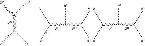
Figure 11: Processes for the production of Higgs bosons at $e^{+}e^{-}$ linear colliders.

The phenomenology of Higgs bosons at both hadron and $e^{+}e^{-}$ colliders has been reviewed in the useful book [129] and, more recently, in the survey [130]. At $e^{+}e^{-}$ colliders, the most promising processes for the production of Higgs bosons are those shown in Figure 11. All three of these processes involve the $ZZh$ and $WWh$ couplings. Above $E_{\hbox{\scriptsize CM}}=1$ TeV, the $Z$ and $W$ fusion processes have large cross sections, of order 100 fb [131]. However, at energies below 500 GeV, and for Higgs-boson masses below 300 GeV, the process $e^{+}e^{-}\to Zh$ has a cross section of 40–80 fb (0.2 R), comparable to that of the fusion process. It also offers distinct experimental advantages: The $Z$ boson can be reconstructed, and then the Higgs boson can be identified, independent of its decay mode, as the state recoiling against it. For Higgs bosons lighter than 200 GeV, it is better to run the machine at lower energies (say, $\sqrt{s}=300$ GeV) to increase the cross section for this process. We will see that this technique allows the identification of the Higgs boson, the measurement of its crucial coupling to $ZZ$, and the systematic study of its decay branching ratios.

We will not discuss in detail the case of Higgs bosons of mass 200–700 GeV, since this situation is not favored in any model of electroweak symmetry breaking. Nevertheless, it is quite straightfoward to find a Higgs boson in this mass range, both at $e^{+}e^{-}$ and at hadron colliders. Such a Higgs decays dominantly to $WW$ and $ZZ$, in a 2:1 ratio of branching fractions. At an $e^{+}e^{-}$ collider, the weak bosons can be reconstructed in their hadronic modes. A data sample of 60 fb^-1 at $E_{\hbox{\scriptsize CM}}=1$ TeV is quite sufficient to discover a 500 GeV Higgs boson [132, 133]. The more difficult case of a very heavy Higgs boson will be discussed in Section 7.2.

Higgs bosons can also be created at hadron colliders, through a variety of production mechanisms. A Higgs boson in the mass range 150–700 GeV can be found straightforwardly in the decay $h^{0}\to ZZ\to 4$ leptons. For Higgs boson masses in the lower range favored by weak-coupling theories, the hadron experiments are most sensitive to Higgs bosons produced through gluon fusion and decaying by $h^{0}\to\gamma\gamma$. The ATLAS and CMS detectors at the LHC will have impressive capabilities to see this $\gamma\gamma$ decay even in the high luminosity environment [4, 5]. With 100 fb^-1 of data, a year’s running at the design luminosity, they should discover the standard model Higgs boson. These experiments also can find at least one Higgs scalar over most of the parameter space of the MSSM by combining many different signatures, such as $h^{0}\to\gamma\gamma$, $A^{0},H^{0}\to\tau^{+}\tau^{-}$, $H^{0}\to 4\ell$. On the other hand, only in a limited region of the parameter space of the MSSM can one observe a Higgs decay that involves the coupling of Eq. 25; thus, it is unlikely that we could establish at the LHC that the new particle discovered in this way is indeed responsible for generating the $W$ and $Z$ masses.

5.2 Detection of Light Higgs Bosons

The Higgs boson of the minimal standard model, in the mass range below 140 GeV, decays mainly into $b\overline{b}$. With smaller branching fractions, it also decays into $WW^{*}$, $\tau\tau$, $c\overline{c}$, $gg$. (The mode $WW^{*}$ refers to one $W$ on-shell and one virtual $W$ observed as $q\overline{q}$ or $\ell\nu$.) The branching fraction into $\gamma\gamma$ is of order $10^{-3}$, which is probably too small to allow observation of this mode in $e^{+}e^{-}$ annihilation. (See, however, Section 5.4.) This general pattern also holds for light scalar bosons in more general models [129]. In this subsection, we will mainly focus on the observation of a light boson $h$ in the $b\overline{b}$ final state. Other decay modes are discussed in Section 5.3.

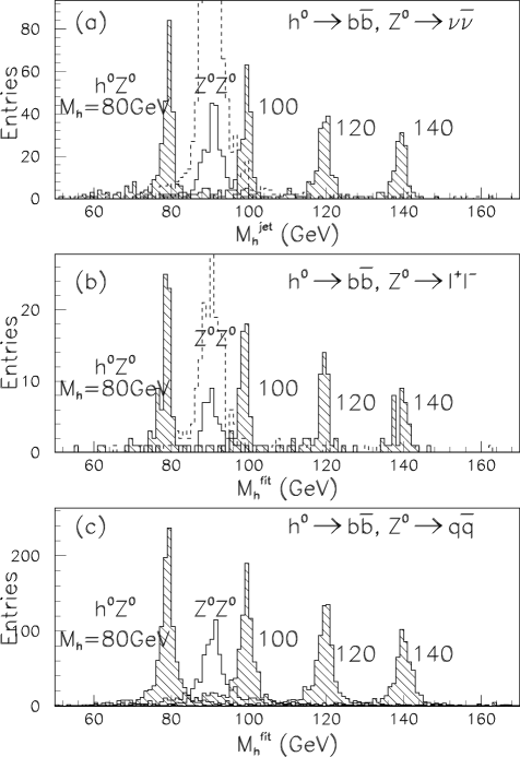
Figure 12: Simulation of the detection of the Higgs boson in the process $e^{+}e^{-}\to Z^{0}h^{0}$, from [42]. The various hatched peaks show the signal expected for a series of values of the Higgs-boson mass from 80 GeV to 140 GeV. The $h^{0}$ is assumed to decay dominantly to $b\overline{b}$; the three figures show the cases of $Z^{0}$ decay to (a) $\nu\overline{\nu}$, (b) $l^{+}l^{-}$, and (c) $q\overline{q}$. The dashed and solid unhatched peaks show the standard-model background without and with a $b$ lifetime cut. The simulation assumes 30 fb^-1 of data at 300 GeV in the center of mass.

It is a remarkable feature of the $Zh$ production process that one can use all three types of $Z$ decay modes—$l^{+}l^{-}$, $\nu\overline{\nu}$ and $q\overline{q}$. Thus, this process gives three independent signals of the discovery. Figure 12 shows simulation results, taken from [42], for the searches in all three final states, assuming the Higgs couplings of the minimal standard model. The main backgrounds are $WW$, $ZZ$, $q\overline{q}$, $t\overline{t}$, $e\nu W$, $\nu\overline{\nu}Z$ final states. The $l^{+}l^{-}b\overline{b}$ mode has the lowest cross section; here, $ZZ$ is the main background, and can be discriminated from the signal in the recoil mass distribution (or, equivalently, in the $E_{l^{+}l^{-}}$ distribution) as long as $|m_{h}-m_{Z}|\mathrel{\mathchoice{\lower 3.0pt\vbox{\halign{$\m@th\displaystyle\hfill#\hfil$\cr>\crcr\sim\crcr}}}{\lower 3.0pt\vbox{\halign{$\m@th\textstyle\hfill#\hfil$\cr>\crcr\sim\crcr}}}{\lower 3.0pt\vbox{\halign{$\m@th\scriptstyle\hfill#\hfil$\cr>\crcr\sim\crcr}}}{\lower 3.0pt\vbox{\halign{$\m@th\scriptscriptstyle\hfill#\hfil$\cr>\crcr\sim\crcr}}}}10$ GeV. In the $\nu\overline{\nu}b\overline{b}$ final state, the signal can be seen in the $m_{jj}$ distribution, again if $m_{h}$ is not too close to $m_{Z}$. If we use four-jet final states, or if $m_{h}\simeq m_{Z}$, $b$-tagging is necessary to reduce the backgrounds. Even in the worst case, and with a cross section of about 150–200 fb at $\sqrt{s}=300$ GeV, it was shown that an integrated luminosity of 1 fb^-1 is already more than enough for the discovery [134]. It is noteworthy that a Higgs boson that decays invisibly can be detected with the same analysis in the $Z\rightarrow l^{+}l^{-}$ channel.

The mass of the Higgs boson can be determined from the di-jet invariant mass of $b\overline{b}$ system, or, more accurately, by the recoil mass in the process with $Z\rightarrow l^{+}l^{-}$. With the capabilities of existing detectors, it is possible to measure $m_{h}$ to 180 MeV with 50 fb^-1 of data [134].

Once the Higgs boson has been found and its mass determined, we would like to establish that this particle is indeed associated with a field that obtains a vacuum expectation value and contributes to the $W$ and $Z$ masses. The general method that answers this question was discussed in the previous subsection. We need to measure the form and strength of the $ZZh$ coupling, which can be inferred from the cross section and angular distribution of the discovery reaction $e^{+}e^{-}\to Zh$. The angular distribution predicted for the coupling given in Eq. 25 is

$${d\sigma\over d\cos\theta}\sim 2+\beta_{Z}^{2}\gamma_{Z}^{2}\sin^{2}\theta\ .$$ (27)

where $\beta_{Z}$, $\gamma_{Z}$ are the velocity and boost of the final-state $Z$. In the high-energy limit, this distribution tends to $\sin^{2}\theta$. This is the characteristic angular distribution of the production of a pair of scalars in $e^{+}e^{-}$ annihilation. It indicates that the $h$ is being produced in association with the Goldstone boson that is eaten to form the longitudinal $Z$. Since the $Z$ is reconstructed, its longitudinal polarization can be verified directly from the angular distribution of its decay into leptons or jets. The angular distributions are described in detail in [135]. The process has a small polarization asymmetry, proportional to $(1-4\sin^{2}\theta_{w})$, which establishes that the the $h$ is produced through a virtual $Z^{0}$. Finally, the total cross section can be measured independently of any assumption about the branching ratios of $h$ by using the leptonic decays modes of the $Z$. This should give a measurement of the $ZZh$ coupling to 4% accuracy with 50 fb^-1 of integrated luminosity [134]. By comparing the cross-section normalization to the prediction from Eq. 25, we can see whether the $h$ field is responsible for the whole $Z$ mass, as in the minimal standard model, or only for a part of it.

The cross sections for production of the MSSM Higgs bosons are presented in [136]. If the heavier scalar Higgs $H^{0}$ is relatively light, the $Z$ receives only a fraction of its mass from the $h^{0}$, and the cross section is correspondingly suppressed. In the region where this suppression is large, the $H^{0}$ should also be within the reach of a 500 GeV collider. Since the $H$ field has the vacuum expectation value which contributes the remainder of the $Z$ mass in this model, the sum of the cross sections into the final states $Zh$ and $ZH$ is approximately the same as the $Zh$ production cross section in the minimal standard model. The analysis in [134] shows that in this case one can find two clear peaks due to $h^{0}$ and $H^{0}$ in the recoil mass distribution.

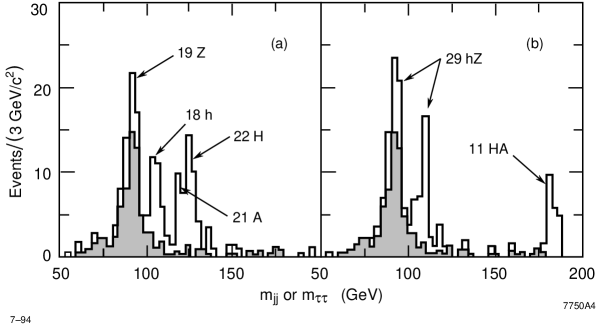
Figure 13: Reconstructed masses of Higgs and $Z^{0}$ bosons, in an analysis optimized to identify the process $e^{+}e^{-}\to b\overline{b}\tau^{+}\tau^{-}$, from [134]. The simulation assumes 10 fb^-1 of data at 400 GeV in the center of mass. The two figures correspond to (a) $m_{A}=120$ GeV, (b) ; $m_{A}=180$ GeV. The shaded area shows the standard-model background, which comes dominantly from $e^{+}e^{-}\to Z^{0}Z^{0}$.

If $H^{0}$ is heavier, it essentially does not contribute to the $Z$ mass, and the properties of the $h$ revert to those of the Higgs boson of the minimal standard model. In this limit, the four states $H^{0}$, $A^{0}$, $H^{+}$ and $H^{-}$ become almost degenerate, and can be looked for in the final states $H^{0}A^{0}$ and $H^{+}H^{-}$. Their decay branching fractions are sensitive functions of many parameters; they depend on $\tan\beta$, on whether decay into top quark pairs is kinematically allowed, and on whether they can decay into neutralinos or charginos. The possible decay modes include: $H^{0}\rightarrow ZZ^{(*)}$, $H^{0},A^{0}\rightarrow b\overline{b}$, $\tau^{+}\tau^{-}$, $t\overline{t}$, $\tilde{\chi}_{1}^{0}\tilde{\chi}_{1}^{0}$, $\tilde{\chi}_{1}^{+}\tilde{\chi}_{1}^{-}$, $\tilde{t}\tilde{t}^{*}$, $H^{+}\rightarrow c\overline{s}$, $t\overline{b}$, $\tilde{\chi}_{1}^{+}\tilde{\chi}_{1}^{0}$, $\tilde{t}\tilde{b}^{*}$. Separate searches have to be performed for each cases, but the studies have shown no problems in looking for these final states. Simulation studies of the detection of the charged Higgs boson are presented in [137, 138]. A particularly interesting case for the neutral bosons is that in which the $A^{0}$ mass is below 200 GeV, and there are no exotic modes which compete with the decays into $b\overline{b}$ and $\tau^{+}\tau^{-}$. In that case, a set of cuts that isolate the $b\overline{b}\tau^{+}\tau^{-}$ final state should show all four neutral Higgs bosons in the same analysis [134]. Simulation results for this case are shown in Figure 13.

5.3 Measurement of the Higgs-Boson Couplings

Once a Higgs boson is discovered and has been confirmed to play a role in the mass generation for $Z$ and $W$, it is also interesting to test whether it is responsible for the masses of the quarks and leptons. This can be done by measuring its couplings to $t$, $b$, $\tau$, etc. The possible variation of these couplings within the MSSM is discussed in [139, 140]; more general models of the Higgs sector allow even a wider variation.

First of all, one can measure relative branching ratios of the Higgs boson. Table 2 shows the expected accuracy of relative branching ratio measurements with 50 fb^-1, from the study [141]. The $b$ branching fraction is expected to be dominant for a light Higgs. It is straightforwardly obtained by vertex tagging. The vertex detector is assumed to be of the quality of the current SLD vertex detector. The $\tau$ branching ration is expected to be about 6% of the $b$ branching fraction; it can be obtained experimentally by selecting events with isolated tracks.

The $WW^{*}$ mode, in which the Higgs boson decays to one $W$ on-shell and one virtual $W$ [142], requires a more subtle analysis. In the minimal standard model, the branching ratio for this mode rises from 1% to 40% over the mass range from 100 to 140 GeV. The most powerful technique for measuring this branching ratio involves dividing the event into six jets, selecting events in which no pair of jets is too close in angle. Then the jets are combined in pairs to find a combination consistent with the $Z$ mass and a combination consistent with the $W$ mass. The remaining two jets give a distribution in jet-jet invariant mass peaked below its kinematic limit of $(m_{h}-m_{W})$. This signal appears on a background of twice the number of events which is roughly flat in this variable. The definite Higgs boson mass or $Z$ recoil energy provides a cross-check to the analysis.

The $c\overline{c}$ and $gg$ decay modes of the Higgs boson, which have branching fractions at the few-percent level, can be recognized as decays to jets that do not contain particles with the characteristically long $b$ lifetimes. It is challenging to separate the charm contribution on the basis of lifetime given the large background from decays to $b\overline{b}$, and this was not attempted in [141]. Techniques for improving the accuracy claimed in Table 2, and possibly resolving the the $c\overline{c}$ mode, are discussed in [144].

Table 2: The errors in relative branching fraction measurement,[141] calculated assuming Standard Model coupling for the Higgs boson and 50 fb^-1 of integrated luminosity at $\sqrt{s}=400$ GeV.

	$m_{h}=140$ GeV	$m_{h}=120$ GeV
Relative Branching Fraction	Expected error	Extrapolated error
$h\rightarrow b\overline{b}$	$\pm 12$ %	$\pm 7$ %
$h\rightarrow WW^{*}$	$\pm 24$ %	$\pm 48$ %
$h\rightarrow c\overline{c}+gg$	$\pm 116$ %	$\pm 39$ %
$h\rightarrow\tau^{+}\tau^{-}$	$\pm 22$ %	$\pm 14$ %

So far, we have discussed only the measurement of Higgs boson branching fractions. However, it is also possible to obtain the total width of a Higgs boson $h$ by combining various measurements that we have discussed. We have explained in the previous section that the $ZZh$ coupling can be determined from the total production cross section. At the same time, the branching ratio for $h^{0}$ to $ZZ^{*}$ can be found from the measurement of the branching ratio to $WW^{*}$ and the relation 26. By comparing these values, one finds the total width of the $h^{0}$ to an accuracy comparable to the accuracy with which the $WW^{*}$ branching ratio has been determined.

Finally, it is possible to measure the Yukawa coupling of $h^{0}$ to the top quark, thereby testing whether the top quark mass originates from the Higgs vacuum expectation value. For the light $h^{0}$ under discussion, the most promising process is $e^{+}e^{-}\rightarrow t\overline{t}h^{0}$ [145] which has a cross section of a few fb. It can determine the $h^{0}t\overline{t}$ coupling to 20% accuracy with 50 fb^-1. We have also noted at the end of Section 4.2 that the measurement of the total cross section for $t\overline{t}$ production in the threshold region can provide an independent measurement of this coupling with comparable accuracy.

5.4 Measurement of the Higgs-Boson Coupling to $\gamma\gamma$

The Higgs decay width into $\gamma\gamma$ and $gg$ is of special interest since it appears at the one-loop level. Thus, any particles which obtain their masses from electroweak symmetry breaking can contribute in the loop. It happens that the dominant contributions come from particles too heavy to appear in direct decays of the $h^{0}$ [129, 146]. Therefore, the measurement of these widths can signal the existence of new heavy particles. Since the branching ratio for $h^{0}\to\gamma\gamma$ is expected to be of order $10^{-3}$, this process is unlikely to be measured through $h^{0}$ production in $e^{+}e^{-}$ annihilation. However, using the $\gamma\gamma$ collider mode discussed in Section 2.4, the Higgs boson can be produced as an $s$-channel resonance decaying, for instance, into $b\overline{b}$. The cross section is proportional to the combination $\Gamma(h\to\gamma\gamma)\cdot BR(h\to b\overline{b})$. The branching ratio will already have been determined in $e^{+}e^{-}$ annihilation. More important, the mass of the $h^{0}$ will already be known from $e^{+}e^{-}$ experiments, and we can tune the energy of the $\gamma\gamma$ collider so that the photon-photon luminosity spectrum peaks at $m_{h}$.

The main background to the Higgs signal is the continuum production of $b\overline{b}$. However, helicity conservation implies that, for the photon helicities $(+,+)$ and $(-,-)$ that produce a $J=0$ resonant state, the $b\overline{b}$ cross section is suppressed by the factor $m_{b}^{2}/s$. This virtue is somewhat diluted by the resolved-photon process [147] in which a gluon from the photon structure function produces $b\overline{b}$, and by continuum production with radiation of an additional gluon [148, 149]. However the study of [148] showed that the Higgs signal can still be observed well above the background.

Simulation studies of the Higgs-boson reconstruction were performed in [53, 150, 151]. In [53], it was found that the reaction $e\gamma\to eZ$, with an initial electron from the Compton-scattered beam, is an important background for Higgs-boson masses below 150 GeV. To suppress this background, a magnetic field must be introduced to displace the scattered electron beam away from the photon-photon collision point. When that is done, the $\gamma\gamma\to h^{0}$ signal stands out above the remaining background processes. The total cross section can be measured at the 6–10% level with 20 fb^-1. As a benchmark, this is sufficient to exclude the contribution of a fourth generation of quarks to the decay vertex at the $5\sigma$ level.

For Higgs bosons heavier than $2m_{Z}$, this cross section can be measured with 10% accuracy in a similar sample by reconstructing the $h^{0}$ from the decay $h^{0}\to ZZ$ [53]. However, as the mass of the Higgs is increased further, the signal gradually disappears below the background due to the reaction $\gamma\gamma\to ZZ$, which appears at the one-loop level in the electroweak theory, and is lost altogether for $m_{h}>350$ GeV [152].

If the Higgs boson is in the low-mass range, it is also most likely to be observed at the LHC in its $\gamma\gamma$ decay mode. Thus, it is worthwhile to say a few words about the comparison of the $e^{+}e^{-}$ and $pp$ measurements. In the $pp$ experiments, the Higgs boson will be produced dominantly via $gg\to h^{0}$; thus the measured rate is proportional to the quantity

$$\Gamma(h^{0}\to gg){1\over\Gamma_{\mbox{\rm tot}}(h^{0})}\Gamma(h^{0}\to\gamma\gamma)\ .$$ (28)

In principle, this measurement could agree with the prediction of the minimal standard model, but there is information in any discrepancy. From this one measurement, however, it is unclear which of the three factors in Eq. 28 is responsible for the deviation. The observable cross section for the $\gamma\gamma$ signal at the LHC varies from a few fb to over 100 fb over the parameter space of the MSSM, or even over that part of the parameter space in which the $h^{0}$ is inaccessible at LEP II [153]. From one number, it is difficult to learn the correct story. However, by combining this number with the values of the second and third factors in Eq. 28—measured respectively in $e^{+}e^{-}$ and $\gamma\gamma$ experiments—and with information on exotic channels of Higgs decay, one can assemble the complete picture of the Higgs boson couplings [130].

For heavier Higgs bosons, the $\gamma\gamma$ process has another virtue: It can make use of the full center-of-mass energy of the collision to produce a single Higgs boson. This is especially attractive in the search for heavy Higgs states in the extended Higss models such as the MSSM. If the heavy Higgs states lie well above $m_{Z}$, then in the $e^{+}e^{-}$ mode they are produced only in pairs, $H^{0}A^{0}$ or $H^{+}H^{-}$. On the other hand, $H^{0}$ and $A^{0}$ can be produced as $s$-channel resonances in the $\gamma\gamma$ mode. The same analysis as the $h^{0}$ case applies if they primarily decay into $b\overline{b}$. Simulation studies are needed for the other possible decay modes such as $t\overline{t}$ or $hh$. It is also possible that the heavy Higgs states may decay mainly invisibly into neutralinos, as emphasized in [154]

Finally, the production of Higgs bosons at a $\gamma\gamma$ collider offers a special experimental handle to determine whether a particular Higgs boson is CP-even or CP-odd [155, 156]. If $\vec{E}$ and $\vec{B}$ are the electromagnetic field strengths, a CP-even Higgs boson couples to the combination $(E^{2}-B^{2})$ while a CP-odd Higgs boson couples to $(\vec{E}\cdot\vec{B})$. The first of these structures couples to linearly polarized photons only if the polarizations are parallel, the latter only if the polarizations are perpendicular. If a particular Higgs boson is a mixture of CP-even and CP-odd components, as can occur in models in which there are new sources of CP-violation in the Higgs sector [157], the interference of these terms gives rise to an asymmetry in the total rate for Higgs production between the helicity states $(+,+)$ and $(-,-)$ [155]. Polarization asymmetries of this sort could be studied at interesting levels with event samples of about 100 fb^-1.

6 SUPERSYMMETRY

Though it is appealing that the electroweak symmetry should be broken by expectation values of scalar fields, it is very difficult to build a fundamental theory which includes this mechanism. In an ordinary scalar field theory, loop diagrams give additive contributions to the scalar mass, and thus the (mass)² of a scalar field naturally is driven to a value of order $\alpha M^{2}$, where $M$ is the largest scale in the theory. In a grand unified theory, $M$ is of order the unification or even the Planck scale. Any scalar field with such enormous mass is irrelevant to electroweak symmetry breaking.

The only known solution to this problem is that of postulating an underlying symmetry that links bosons and fermions, supersymmetry. In the standard model, the fermions are forbidden from obtaining mass except through $SU(2)\times U(1)$ breaking. In a supersymmetric model, this is also true for scalar fields in the model, and so it is possible for elementary Higgs scalar particles to naturally remain at the weak scale rather than being driven to up to the unification scale.

We have no space for a full review of supersymmetric models here. Excellent reviews can be found in [158, 159, 160, 161, 162]. We should, however, point out two serendipitous features of supersymmetric models of particle interactions. The first comes in the relation among the standard-model coupling constants. The simplest grand unification models predict a relation between $\alpha$, $\alpha_{s}$, and $\sin^{2}\theta_{w}$ that is not obeyed by the values of these quantities measured in the precision experiments at LEP. However, the assumption that the supersymmetric partners of the known particles appear at the weak scale changes the extrapolation to large scales and results in a successful prediction. The current status of this prediction is reviewed in [163].

The second success of supersymmetric models comes in providing a mechanism for electroweak symmetry breaking. To explain this phenomenon, one must explain why it is that the Higgs boson (mass)² is not only small but also negative. In supersymmetric models, one of the Higgs mass parameters receives a negative correction from loop diagrams proportional to the top-quark Higgs coupling. Thus, if the top quark is the heaviest standard particle, the Higgs field potential energy naturally has a symmetry breaking form. This phenomenon is reviewed in [164].

An important consequence of this mechanism is that the $Z$ and $W$ masses become connected to the scale of superpartner masses. Unless there is a fine adjustment of parameters to make the $Z$ and $W$ masses especially small, these mass would be expected to be roughly equal to the masses of the $W$, $Z$, and Higgs superpartners. Several groups have tried to make this connection quantitative and have used it to bound the masses of supersymmetric particles [165, 166, 167]. Among their limits are bounds on the masses of the $W$ and gluon partners

$$m(\widetilde{w})\mathrel{\mathchoice{\lower 3.0pt\vbox{\halign{$\m@th\displaystyle\hfill#\hfil$\cr<\crcr\sim\crcr}}}{\lower 3.0pt\vbox{\halign{$\m@th\textstyle\hfill#\hfil$\cr<\crcr\sim\crcr}}}{\lower 3.0pt\vbox{\halign{$\m@th\scriptstyle\hfill#\hfil$\cr<\crcr\sim\crcr}}}{\lower 3.0pt\vbox{\halign{$\m@th\scriptscriptstyle\hfill#\hfil$\cr<\crcr\sim\crcr}}}}250\hbox{\rm GeV}\ ,\qquad m(\widetilde{g})\mathrel{\mathchoice{\lower 3.0pt\vbox{\halign{$\m@th\displaystyle\hfill#\hfil$\cr<\crcr\sim\crcr}}}{\lower 3.0pt\vbox{\halign{$\m@th\textstyle\hfill#\hfil$\cr<\crcr\sim\crcr}}}{\lower 3.0pt\vbox{\halign{$\m@th\scriptstyle\hfill#\hfil$\cr<\crcr\sim\crcr}}}{\lower 3.0pt\vbox{\halign{$\m@th\scriptscriptstyle\hfill#\hfil$\cr<\crcr\sim\crcr}}}}800\hbox{\rm GeV}\ ,$$ (29)

for some reasonable limits on allowable fine adjustment. This argument implies that the superpartners should be found at the next generation of high-energy colliders.

In addition to being well-motivated, supersymmetric models have another importance for understanding the role of future colliders. Because these theories contain only weak-coupling phenomena, we can analyze their consequences in detail by direct calculation. This allows us to appreciate, in a way that is not possible for theories with strong-coupling dynamics, the wide variety of phenomena that these models make available to experiment. By showing the level of detail at which we can observe these phenomena, we illustrate the analytic power of linear colliders. If the physics of electroweak symmetry breaking is interesting and complex, even if it is of a different character, we expect that the lessons we learn here will carry over to exploration of the new sector that this implies.

6.1 The Experimental Investigation of Supersymmetry

The basic implication of supersymmetry is that each particle in Nature is accompanied by a particle with the same standard model quantum numbers, differing in spin by ${1\over 2}$ unit. Thus, quarks and leptons have scalar partners (squarks and sleptons), gauge bosons have spin-${1\over 2}$ partners (gauginos), and so forth. If supersymmetry is exact, the partners have the same mass as the original particles, and this is clearly excluded. However, it is reasonable that supersymmetry could be spontaneously broken. In this case, the renormalizable couplings of particles and superpartners will be constrained by the symmetry to be equal to the corresponding standard-model couplings, but the superpartner masses and soft interactions may take a more general form.

Both aspects of supersymmetry theory are important to test in experiments. First, we must find the supersymmetry partners of quarks, leptons, and gauge bosons, and we must verify that they have the quantum numbers and couplings predicted by supersymmetry. Second, we must investigate the properties of the supersymmetry-breaking mass terms and interactions. In most models, these originate at very high scales, and so their measurement can give new information on the nature of the grand unified or other underlying theory. In Sections 6.2 and 6.3, we will discuss techniques for discovering superpartners and measuring their properties at linear colliders. In Section 6.4, we will discuss the signficance of these measurements for tests of unifying theories.

Hadron colliders are also powerful tools for discovering supersymmetric particles, particularly the squarks and gluinos which are produced with large cross section in gluon-gluon collisions. Reviews of the expectations for supersymmetry experiments at the LHC, for example, can be found in [5, 168, 169, 170]. It is likely that the LHC can observe signatures of a gluino up to gluino masses approaching 2 TeV, well beyond the reach of planned $e^{+}e^{-}$ colliders for any superpartner. However, it is a typical property of models that the squarks and gluinos are much heavier than the color-singlet particles that are easy to study at $e^{+}e^{-}$ colliders. In addition, it is a prediction of the theory that the supersymmetry signatures at $pp$ colliders are complex and difficult to interpret, while supersymmetry phenomena at $e^{+}e^{-}$ colliders are much simpler to study in detail. We will return to this point in Section 6.4.

In this review, we will discuss only the most popular framework for supersymmetry phenomenology. We will assume the minimal particle content (that is, the MSSM) and we will assume the presence of an exact $R$-parity symmetry, under which all of the particles of the standard model have $R=+1$ while their superpartners have $R=-1$. Therefore, the lightest superpartner is stable. Cosmological arguments require this lightest particle to be neutral and make it unlikely to be the sneutrino. Because of our assumption of exact $R$-parity, the superparticles are always produced in pairs. Each decays into the lightest superpartner directly or in a cascade, giving the experimental signature of missing $p_{T}$ and/or large acoplanarity. Models with broken $R$-parity are discussed in [171, 172]; these necessarily involve either lepton or baryon number violation at the weak interaction scale and so give different, but sometimes quite spectacular, signatures.

6.2 Gauge-Boson Superpartners at $e^{+}e^{-}$ Colliders

The naturalness argument leading to Eq. 29 implies that the superpartner of the $W$ boson is likely to be relatively light. Indeed, this particle could well be the lightest charged superpartner and thus an interesting object of study at an $e^{+}e^{-}$ collider.

In supersymmetric models, the $W$ partner ($\tilde{W}$ or “wino”) is generally not a mass eigenstate. Instead, it mixes with another superpartner with the same electric charge, the partner of the charged Higgs boson ($\tilde{H}^{+}$ or “higgsino”). The mass matrix of these fields has the form

$$(\tilde{W}^{-}\,\tilde{H}_{1}^{-})\left(\begin{array}[]{cc}M_{2}&\sqrt{2}m_{W}\sin\beta\\ \sqrt{2}m_{W}\cos\beta&\mu\end{array}\right)\left(\begin{array}[]{c}\tilde{W}^{+}\\ \tilde{H}_{2}^{+}\end{array}\right),$$ (30)

where the fermion fields $\tilde{W}^{\pm}$, $\tilde{H}^{\pm}$ are left-handed spinors, $M_{2}$ is the $SU(2)_{L}$ gaugino mass, $\mu$ is the supersymmetic Higgs mass term, and $\tan\beta$ is the vacuum angle defined in the previous section. The eigenstates are called “charginos” and denoted $\tilde{\chi}_{1,2}^{\pm}$ for the lighter and heavier states, respectively. If $\mu\gg M_{2}$, $\tilde{\chi}_{1}^{\pm}$ is to a good approximation a wino of mass $M_{2}$. If $M_{2}\gg\mu$, $\tilde{\chi}_{1}^{\pm}$ is approximately a higgsino of mass $|\mu|$. If $(M_{2}-|\mu|)$ is of order $m_{W}$, the mass eigenstates are mixtures of the two. This occurs in a relatively large part of parameter space for charginos light enough to be found at LEP II, but only in a more limited region for heavier charginos.

In a similar way, the superpartners of the photon and $Z$ mix with the partners of the two neutral Higgs boson fields. This leads to a $4\times 4$ mixing problem in the space of the four fields $(\tilde{B},\tilde{W}^{0},\tilde{H}_{1}^{0},\tilde{H}_{2}^{0})$, where $\tilde{B}$, $\tilde{W}^{0}$ denote the superpartners of the $U(1)$ and neutral $SU(2)$ gauge bosons. The four mass eigenstates are called “neutralinos” and denoted by $\tilde{\chi}_{1,2,3,4}^{0}$ from the lightest to the heaviest.

To reduce the number of parameters on which the chargino and neutralino masses depend, the assumption is often made that the gaugino masses are in the ratio of the corresponding gauge coupling constants:

$$\frac{M_{1}}{\alpha_{1}}=\frac{M_{2}}{\alpha_{2}}=\frac{M_{3}}{\alpha_{3}},$$ (31)

where $\alpha_{1}=\frac{5}{3}\alpha/\cos^{2}\theta_{W}$. This relation follows from the assumption that the three gauginos are unified into a single multiplet with a common mass at the grand-unification scale. We will use this relation as a convenient reference point in our discussion, but one should not forget that it is important also to test it experimentally. Using this assumption to eliminate $M_{1}$, we can write the mass matrices both for charginos and neutralinos in terms of the three parameters $M_{2}$, $\mu$, and $\tan\beta$. Then, in the two limiting cases just described for charginos, the neutralinos have the following spectrum: In the case $\mu\gg M_{2}$, the lightest two neutralinos are approximately $\tilde{B}$, with mass $M_{1}\approx{1\over 2}M_{2}$, and $\tilde{W}^{0}$, with mass $M_{2}$. In the case $M_{2}\gg\mu$, the two light neutralinos are approximately higgsinos, both with mass close to $|\mu|$.

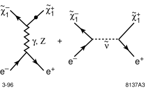
Figure 14: Feynman diagrams for chargino pair production.

The charginos are pair-produced in $e^{+}e^{-}$ annihilation through the diagrams shown in Figure 14. The amplitude receives contributions from $s$-channel $\gamma$ and $Z$ exchange, and from $t$-channel $\tilde{\nu}_{e}$ exchange. The first of these processes is present for both electron polarization states, but the $\tilde{\nu}_{e}$ exchange is present only for left-handed electrons, since the vertex is related to the usual weak-interaction vertex by supersymmetry. The production cross section is of order 100 fb from an $e^{-}_{R}$ beam and of order 1000 fb from an $e^{-}_{L}$ beam, with some destructive interference if the $\tilde{\nu}_{e}$ is in the same mass region. A very useful compilation of the formulae for this and other supersymmetry production processes in $e^{+}e^{-}$ annihilation is given in [173].

The chargino decay depends both on the makeup of the mass eigenstate and on the masses of other superpartners. If the decay $\tilde{\chi}_{1}^{\pm}\rightarrow\tilde{\chi}_{1}^{0}W^{\pm}$ is kinematically allowed, this channel usually dominates. Then the ratio of leptonic and hadronic final states is determined by the $W$ branching fractions, and it is possible to reconstruct the $W$ from its 2-jet decay. If this mode is forbidden, $\tilde{\chi}_{1}^{\pm}$ decays into three-body final states $l\nu\tilde{\chi}_{1}^{0}$ and $q\overline{q}\tilde{\chi}_{1}^{0}$. The amplitudes contain both off-shell $W$-exchange as well as slepton or squark exchanges, and the decay branching ratios are sensitive function of their masses.

The detection of chargino pair-production is quite straightforward. One selects events with large missing energy, large acoplanarity to eliminate background from two-photon events, and sufficient visible energy to be inconsistent with $e^{+}e^{-}\to e\nu W$. These cuts eliminate most of the background from $e^{+}e^{-}\to W^{+}W^{-}$, and tighter kinematic cuts can be placed if necessary. An explicit simulation is described in [174]; the cuts suggested there have an efficiency of 25% in the case where both charginos decay hadronically and 10% if one chargino decays leptonically. The discovery reach with 20 fb^-1 is almost indistinguishable from the kinematic limit over most of parameter space, unless $m(\tilde{\nu}_{e})\sim E_{\hbox{\scriptsize CM}}/2$. Once the chargino is found, we will discover whether or not it decays to an on-shell $W$; then one can optimize the cuts for higher efficiency to study the properties of this particle.

The mass of the chargino can be measured by selecting events with one hadronic and one leptonic decay and identifying the endpoints of the 2-jet energy distribution. These endpoints directly reflect the kinematics of the decay $\tilde{\chi}_{1}^{\pm}\to q\overline{q}\tilde{\chi}_{1}^{0}$ and thus determine both $m(\tilde{\chi}_{1}^{\pm})$ and $m(\tilde{\chi}_{1}^{0})$. Figure 15 shows a simulation study of this measurement [175]; for that set of parameters, both masses are determined at the 3% level with 20 fb^-1 of data. At the same time, one can compare the production rates for hadronic and leptonic decays and determine the relative branching ratio. Since these two are the only available channels, one can derive from this the absolute branching fractions and the total cross section for chargino production.

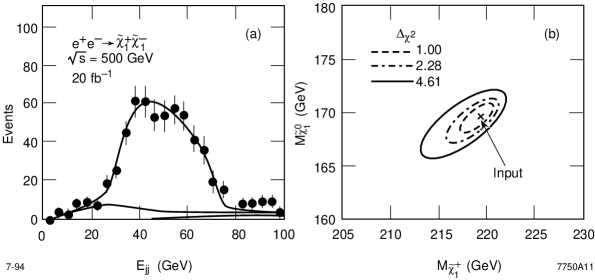
Figure 15: Chargino mass measurement, from [175]: (a) Di-jet energy distribution from chargino pair production, (b) $\chi^{2}$ contours for the fit to the $\tilde{\chi}_{1}^{\pm}$ and $\tilde{\chi}_{1}^{0}$ masses. A sample parameter set $M_{2}=400$ GeV, $\mu=250$ GeV, $\tan\beta=2$ was chosen.

However, the measurement of the mass of the $\tilde{\chi}_{1}^{\pm}$ is only the beginning of what is needed to understand the physics of the gauge-boson partners. We have seen that the lightest chargino is in general a mixture of wino and higgsino components; to completely determine the chargino state, we must find the mixing angles. This is not a purely academic problem, for two reasons. First, the mixing angles are functions of the underlying parameters $(M_{2},\,\mu,\,\tan\beta)$, and their measurement can play a major role in determining these parameters. More importantly, all heavier superparticles will eventually decay into charginos and neutralinos, and thus the observable signatures of their decays will be determined by the chargino and neutralino mixing pattern.

Fortunately, we have by no means exhausted the tools available to us in $e^{+}e^{-}$ annihilation. Consider, for example, measuring the cross section for chargino pair production from a right-handed electron beam. For this initial state, the sneutrino diagram in Figure 14 vanishes. But also the $s$-channel diagram in this figure undergoes some simplification. If, for a moment, we ignore the $Z$ mass and convert the $\gamma$ and $Z$ to $SU(2)\times U(1)$ states, the $e^{-}_{R}$ couples only to the $U(1)$ gauge boson. This, in turn, does not couple to the $\tilde{W}^{\pm}$ but only to the $\tilde{H}^{\pm}$. Thus, the diagrams for chargino pair production couple only to the higgsino components of the chargino. Actually, since the mass matrix 30 is not symmetric, it requires two mixing angles, one for $\tilde{\chi}^{+}_{1L}$, one for $\tilde{\chi}^{-}_{1L}$. The first of these angles gives the cross section for backward $\tilde{\chi}_{1}^{+}$ production, the second for forward $\tilde{\chi}_{1}^{+}$ production. By measuring the cross section and the forward-backward asymmetry, both mixing angles can be determined.

The realization of this strategy does not require asymptotic conditions. For a 200 GeV chargino at $E_{\hbox{\scriptsize CM}}=500$ GeV, the cross section for $e^{-}_{R}e^{+}\to\tilde{\chi}_{1}^{+}\tilde{\chi}_{1}^{-}$ varies from zero to 150 fb as one moves from the pure wino to pure higgsino case. The forward-backward asymmetry of $\tilde{\chi}_{1}^{+}\tilde{\chi}_{1}^{-}$ production cannot be measured directly because each chargino decays to an unobserved neutralino. It is possible to approximate this observable, however, by selecting events with one hadronic and one leptonic decay and measuring the forward-backward asymmetry of the $q\overline{q}$ system. In practice, one must impose a cut to remove events in which the total momentum of the $q\overline{q}$ system has $\cos\theta>0.8$ to suppress background from $W$ pair production. Even with this restriction, it was shown by simulation that this quantity is highly correlated with the forward-backward asymmetry of the chargino pairs [176]. In that study, a point in parameter space was chosen where the chargino $\tilde{\chi}_{2}^{\pm}$ could also be observed, so that the masses of the two charginos and the cross section and forward-backward asymmetry for $e^{-}_{R}e^{+}\to\tilde{\chi}_{1}^{+}\tilde{\chi}_{1}^{-}$ could be used to determine the four parameters in Eq. 30. With 30 fb^-1 of data, the two mixing angles could be independently determined to an accuracy of 5^∘.

A similar analysis applied to the process $e^{-}_{L}e^{+}\to\tilde{\chi}_{1}^{+}\tilde{\chi}_{1}^{-}$ can determine $m(\tilde{\nu}_{e})$. Once the chargino mixing angles are determined, this mass is the only unknown parameter in the formula for the cross section. The sensitivity to the sneutrino contribution at $E_{\hbox{\scriptsize CM}}=500$ GeV extends almost to a sneutrino mass of 1 TeV. Thus, if the lepton partners are not observed at the first stage of the linear collider, this measurement can give an idea of how much the energy must be raised to find them.

We should note that the analyses we have described here assumed that the chargino $\tilde{\chi}_{1}^{\pm}$ is the lightest charged superpartner. The signatures may be more complicated if the chargino is heavy enough to decay into sleptons, e.g., by $\tilde{\chi}_{1}^{\pm}\rightarrow l^{\pm}\tilde{\nu}_{l}$ followed by $\tilde{\nu}_{\ell}\rightarrow\nu_{\ell}\tilde{\chi}_{1}^{0}$. Fortunately, in this case, the charged slepton can always be observed; the mass splitting between the sneutrino $\tilde{\nu}_{\ell}$ and the corresponding slepton $\tilde{\ell}_{L}$ obeys an inequality

$$m^{2}(\tilde{\ell}_{L})\leq m^{2}(\tilde{\nu}_{\ell})+0.77m_{Z}^{2}$$ (32)

which follows directly from supersymmetry and predicts a rather small splitting. In a situation such as this, the best strategy would be to decrease the energy so that only the sleptons could be produced, study these with care, and then use the properties of the final-state sleptons to isolate the charginos. At an $e^{+}e^{-}$ collider, we can always study a novel spectroscopy systematically in this way, gaining precision information about the lightest particles and then using this information to disentangle the complex signatures of the heavier states.

6.3 Quark and Lepton Superpartners at $e^{+}e^{-}$ Colliders

In supersymmetric models, the sleptons often have masses comparable to those of the charginos. Thus, these particles may also be light enough to be observed even at the first stage of the linear-collider program. There are six distinct slepton states, since the left- and right-handed components of $e$, $\mu$, and $\tau$ each have separate superpartners. The $\tau$ partners $\tilde{\tau}_{L}$, $\tilde{\tau}_{R}$ can mix, with an off-diagonal element in the mass matrix proportional to $m_{\tau}$. This effect is unimportant for the electron and muon partners, which are thus associated with definite chirality. The muon and $\tau$ partners are pair-produced by $s$-channel $\gamma$ and $Z$ exchange. For the electron partners, there is another contribution from $t$-channel neutralino exchange. The cross sections are of order 100 fb at $\sqrt{s}=500$ GeV, and can be larger for selectrons due to the $t$-channel contribution. All of the processes have large polarization asymmetries, with the $e^{-}_{R}$ beam favoring $\tilde{\ell}_{R}$ production and vice versa.

If sleptons are lighter than the chargino, they decay directly into leptons and $\tilde{\chi}_{1}^{0}$: $\tilde{\ell}\rightarrow\ell\tilde{\chi}_{1}^{0}$. Even if the sleptons can decay to charginos, the branching ratio into this mode typically remains substantial. The signature of this decay is particularly simple, since it gives acoplanar leptons with no other visible energy. The main background comes from $W$ pairs decaying into leptons and neutrinos.

The discovery of sleptons is relatively easy close to the kinematic limit. The analysis in [177] shows one can discover smuons at the 5 $\sigma$ level up to 225 GeV with a collider of $\sqrt{s}=500$ GeV and an integrated luminosity of 20 fb^-1, as long as the mass difference beween the smuon and the $\tilde{\chi}_{1}^{0}$ is greater than 25 GeV, despite the $\beta^{3}$ threshold behavior of the cross section for scalar particles.

Once the sleptons are discovered, we would like to measure their properties. The mass measurement is very simple. Because the sleptons are scalars and they decay to a two-body final state, the final lepton has a flat energy distribution over the kinematically allowed range

$$\frac{m_{\tilde{\ell}}}{2}\left(1-\frac{m_{\tilde{\chi}_{1}^{0}}^{2}}{m_{\tilde{\ell}}^{2}}\right)\gamma(1-\beta)<E_{l}<\frac{m_{\tilde{\ell}}}{2}\left(1-\frac{m_{\tilde{\chi}_{1}^{0}}^{2}}{m_{\tilde{\ell}}^{2}}\right)\gamma(1-\beta)\,,$$ (33)

where $\beta$ and $\gamma$ are the velocity and boost of the slepton. This distribution has sharp discontinuities at the endpoints, which directly indicate the masses of the slepton and neutralino. A simulation of this measurement for the case of the $\tilde{\mu}_{R}$ is shown in Figure 16 [175]. We see from the $\chi^{2}$ distribution that the masses of the smuon and of the $\tilde{\chi}_{1}^{0}$ are determined to 1% accuracy. The exceptionally low level of background was achieved by employing a right-handed electron beam (assumed to have $P=95$%) to decrease the cross section for $W$ pair production.

Figure 16: Smuon mass measurement, from [175]: (a) Energy distribution of the final muon from $\tilde{\mu}_{R}$-pair production, including standard model backgrounds. (b) $\chi^{2}$ contours for the fit to the $\tilde{\mu}_{R}$ and $\tilde{\chi}_{1}^{0}$ masses.

The angular distribution of sleptons can be inferred from the lepton angular distributions up to a two-fold ambiguity. For the case of smuons, this gives another check of the spin from the characteristic $\sin^{2}\theta$ distribution. For selectrons, the measurement the forward peak due to $t$-channel neutralino exchange can be used as an alternative way to constrain the neutralino mixing problem. At the point in parameter space studied in the simulations of [175], this led to a measurement of the ratio $M_{1}/M_{2}$ with 5% accuracy for a data sample of 50 fb^-1, giving a crucial and necessary test of the grand unification relation, Eq. 31. On the other hand, if the chargino is not found at the first stage of the linear collider, the assumption of Eq. 31 implies an upper bound on the chargino mass, $m(\tilde{\chi}_{1}^{\pm})<2m(\tilde{\chi}_{1}^{0})$, which can be confirmed as the energy of the collider is increased.

An alternative way to study the effects of $t$-channel neutralino exchange is to produce selectron pairs through the reaction $e^{-}e^{-}\to\tilde{e}^{-}\tilde{e}^{-}$. This process also offers an environment with very low background in which to search for the selectron at the extremes of parameter space [178]. Another interesting feature of the $e^{-}e^{-}$ production mode is its ability to search for lepton flavor violation, in the process $e^{-}e^{-}\to\tilde{e}\tilde{\mu}$, at interesting levels [179].

As the sleptons become heavier, the left-handed sleptons may decay into charginos, by $\tilde{\ell}_{L}\rightarrow\nu_{\ell}\tilde{\chi}_{1}^{-}$ or $\tilde{\nu}_{\ell}\rightarrow\ell\tilde{\chi}_{1}^{+}$. In this case, the sneutrino has decays with significant visible energy, making it straightforward to measure its mass accurately [33].

For very heavy sleptons, the $e^{-}\gamma$ collider option can extend the reach for the selectron search beyond that of the $e^{+}e^{-}$ mode. As long as the neutralinos are relatively light, the selectron can be produced in the process $e^{-}\gamma\rightarrow\tilde{e}^{-}\tilde{\chi}_{1}^{0}$ up to 80% of the collider center-of-mass energy. The $\nu_{e}W^{-}$ background to this process can be suppressed by the use of beam polarization [180].

Figure 17: Contributions to the decay $\tilde{\tau}_{R}\to\tau\tilde{\chi}_{1}^{0}$, showing the correlation with $\tau$ polarization.

In the case of the $\tilde{\tau}$, there are two further interesting features. First, as noted above, the mass eigenstates of the $\tilde{\tau}$ can be mixtures of $\tilde{\tau}_{L}$ and $\tilde{\tau}_{R}$. It is possible to measure the mixing angle using the production cross sections from the two polarized beams [181]. Second, the $\tilde{\tau}$ has a additional and wonderful observable, the polarization of the final-state $\tau$ from $\tilde{\tau}$ decay. The $\tau$ polarization can be measured as is done at LEP, from the energy distributions of its $\pi$ and $\rho$ decay products. For the simplest case in which the $\tilde{\tau}$ is pure $\tilde{\tau}_{R}$, the $\tau$ polarization indicates the mixture of gaugino and higgino in the final-state neutralino, as shown in Fig. 17. If the $\tilde{\tau}$ is known from the cross section measurements to be a mixture of components, this can be taken into account in the analysis. Since the size of the $\tau$ coupling to the higgsino depends on $\tan\beta$, this measurement can be used to determine $\tan\beta$ if the neutralino mixing is known from other observations.

Similarly detailed studies can be made for $\tilde{t}$, $\tilde{b}$ and other types of $\tilde{q}$ as well. We refer to [182, 183] for further details.

6.4 Tests of Supersymmetric Unification

One of the wonderful properties of the supersymmetric models is their connection to models of grand unification, and to more ambitious models of gravity and string theory. Thus, the measurements of superparticle masses and properties are important not only in their own right but also as a window into these deep but speculative ideas. Because supersymmetric models are expected to be weakly coupled from the TeV scale to the Planck scale, it is not unreasonable that masses observed in collider experiments can be extrapolated to such high energies. This is a straightforward renormalization-group analysis, which is already know to work well for the values of the standard-model gauge couplings [163]. It is, then, worth reviewing how well we can measure those quantities that are the necessary inputs to this analysis. A more complete discussion of these issues can be found in [184].

First of all, it is important to note that supersymmetry makes quantitative predictions of relations among coupling constants. The experimental verification of these relations would provide important confirmation that the new physics observed at high-energy colliders indeed arises from supersymmetry. At a linear collider, several tests of this type are possible. In the chargino study described in Section 6.2, the determination of the chargino mass matrix leads to a determination of the parameter $m_{W}$ in Eq. 30. This parameter is equal to the $W$ mass by virtue of the equality of the Higgs-Higgs-$W$ coupling and the $h\tilde{H}\tilde{W}$ coupling. It is also possible to test the equality of the $e\nu W$ coupling and the $e\tilde{\nu}\tilde{W}$ coupling. These tests check the supersymmetric coupling constant relations at the 20% level with 100 fb^-1 of data [176]. We know of no comparable experiments that are possible at hadron colliders.

To test the gaugino-mass-unification relation, Eq. 31, and to examine the question of unification relations for the masses of quark and lepton partners, it is necessary to have accurate determinations of the superpartner masses. We have already discussed the mass measurements for color-singlet superpartners. If squarks lie within the energy reach of the linear collider, their masses will also be measured accurately. For gluinos and for heavy squarks, however, we will need to rely on measurements made at the LHC. Using the unification relation Eq. 31, the gluino mass reach of 1.7 TeV quoted in [5] would be equivalent to a $\tilde{\chi}_{1}^{\pm}$ mass of 500 GeV, so that the LHC would cover roughly the same region of the parameter space of a unified model as the linear collider at 1 TeV in the center of mass. We have already noted that the LHC offers powerful capabilities to recognize the supersymmetric particle production, particularly for squark and gluino production. However, the signatures of supersymmetry visible at hadron colliders are, for the most part, integral quantities such as cross sections for missing energy and multilepton events. We know of only one observable in which the gluino produces a peak in a mass distribution [185], and even in that case, the location of the peak relative to the gluino mass is model-dependent. The wealth of data available from supersymmetry observations at the LHC can be used to determine the squark and gluino masses, through experiments described in [5, 169], but the interpretation of these experiments requires knowledge of the decay patterns of the superparticles. In theoretical models, these decay patterns are complicated because they involve cascade decays through the spectrum of charginos and neutralinos [186, 187]. Thus, the measurement of the chargino and neutralino mixing angles at a linear collider will be important in the interpretation of the LHC data. They may be essential for the LHC experiments to produce the precision mass measurements needed for the study of unification.

Figure 18: Test of the mass relation of Eq. 34, assuming 50 fb^-1 of data, from [175].

Once the spectrum of superparticles is known, we will be able to extrapolate the mass pattern to very high energies and look for regularities. We have already mentioned the test of the ratio $M_{1}/M_{2}$ which can be obtained in the study of selectron production. With information from the LHC, we can learn the relation of the gluino to the lighter gauginos. For the quark and lepton partners, a very important question is that of whether the masses are universal among species, or follow some different pattern, when extrapolated to the unification scale. The equality of the $\tilde{e}_{R}$ and $\tilde{\mu}_{R}$ masses at the unification scale implies equality for the physical masses. If this equality is violated even at the level of a few percent, a level of accuracy we have shown should be reached at a linear collider, this strongly constrains sources of lepton flavor violation up to the grand unification scale and actually excludes the simplest $SO(10)$ unified theories. The relation of the left- and right-handed slepton masses is slightly more involved. The masses of the left-handed sleptons receive a radiative correction from the loop diagram which includes a lepton and a wino. This implies that, if the masses of $\tilde{\ell}_{R}$ and $\tilde{\ell}_{L}$ are to be equal at the unification scale, their physical masses must obey the relation

$$m^{2}(\tilde{\ell}_{L})-m^{2}(\tilde{\ell}_{R})=(0.5M_{2})^{2}\ .$$ (34)

The simulation study [175] addressed the question of how well this relation could be tested at a linear collider; the result, for 50 fb^-1 of data, is shown in Figure 18.

Thus, if we are lucky, the discovery of supersymmetry at the next generation of hadron and lepton colliders could be the beginning of a fascinating study of the fundamental structure of the unified theory at very small distances. The linear-collider experiments would have a central role in this investigation.

7 THE HIGGS SECTOR (STRONG COUPLING)

We now turn to models in which electroweak symmetry breaking does not involve a fundamental Higgs boson, but rather is the result of strong-coupling dynamics. This class of models realizes the original notion of Higgs, who imagined gauge symmetry breaking as proceding by a mechanism analogous to that of superconductivity [188]. In this section, we will survey the components of these models and their signatures at linear colliders.

7.1 Strongly Coupled Higgs Sectors

Ideally, we would discuss models with strong-coupling electroweak symmetry breaking in the same way that we discussed supersymmetry in Section 6, by constructing a minimal model with the essential illustrative features of this class and then analyzing the consequences of that model in detail. Unfortunately, for strong-coupling models, an approach of this type is not straightforward. Strong-coupling models of electroweak symmetry breaking divide into classes according to the particular dynamics assumed, and some of these cases can be studied in detail, but in no case is the story as clean as in weak-coupling models.

There is a strong-coupling model whose theoretical basis is well-understood, and which does naturally lead to electroweak symmetry breaking at a scale well below an assumed scale of unification. This is the minimal technicolor model [189, 190], which postulates a new set of strong interactions similar to those of QCD, at an energy scale of roughly 1 TeV. One assumes that this theory has chiral symmetries as in QCD, and that these are broken by the same mechanism, fermion-antifermion pair condensation due to the strong QCD attraction. If the elementary fermions of this new gauge theory are assigned $SU(2)\times U(1)$ quantum numbers similar to those of quarks, this chiral symmetry breaking leads to spontaneous $SU(2)\times U(1)$ breaking, in which the parameters of the symmetry-breaking sector are determined as properties of the technihadrons. For example, the Higgs field vacuum expectation value Eq. 1 is reinterpreted as the pion decay constant $f_{\pi}$ of the new strong interactions. Insofar as this theory exactly mimics the dynamics of QCD, its predictions can be worked out in detail.

On the other hand, the minimal technicolor model does not agree with experiment, for several reasons. First, it contains no mechanism for giving mass to the quarks and leptons. This problem can be solved by introducing additional gauge particles, called extended technicolor (ETC) bosons, which can convert technicolor fermions to ordinary quarks and leptons [17]. However, this modification typically results in unacceptably large predictions for flavor-changing neutral current processes [191, 192], and in a value of the top-quark mass bounded from above at about 100 GeV [193]. In addition, the corrections of this model to precision electroweak physics are large enough to be excluded by the most recent measurements (see, for instance, [15]). As a cure for these problems, most enthusiasts of techhnicolor models would consider the dynamics of technicolor to be rather different from QCD, either a non-asymptotically free gauge theory near an ultraviolet fixed point [194] or an asymptotically free gauge theory with very slow running of the coupling constant (“walking technicolor”) [195]. Because little is known about the dynamics of the underlying gauge theories of these types there is considerable room for assumption or guesswork.

A particularly interesting line of speculation is that the fermions that condense in pairs to break $SU(2)\times U(1)$ are precisely the top and antitop [196, 197, 198]. This idea has given rise to a more general class of models, called topcolor, in which the top quark or the third generation of fermions has special gauge interactions not shared by the lighter fermions [199]. The spectrum of models that realize this idea blends smoothly into the class of technicolor models in which strong ETC interactions enhance the top-quark mass to its observed value [200, 201]. This idea of new gauge forces coupling to the third generation leads to a number of interesting signatures both at hadron and lepton colliders; we will review some of these in Section 7.5.

One might also react to this confusion of models by asking for experiments that are sensitive to new strong interactions in the Higgs sector in a model-independent way. To imagine what such experiments would look like, we can start from the minimal requirement for a theory of electroweak symmetry breaking by strong interactions. Every such theory begins as a strong-interaction theory with a global symmetry $SU(2)\times U(1)$ that is spontaneously broken. When the global symmetry $SU(2)\times U(1)$ is promoted to a local symmetry by coupling in the weak interaction gauge bosons, those particles obtain mass. The observed relation $m_{W}=m_{Z}\cos\theta_{w}$ is not obvious in this general context, but it is imposed straightforwardly [202] if we assume also that the original theory had an $SU(2)$ global symmetry that is unbroken, under which the weak interaction currents form an isotriplet. Then the underlying strong interaction theory has global symmetry $SU(2)\times SU(2)$, spontaneously broken to the “custodial” $SU(2)$. This is just the symmetry structure of QCD with two flavors, and that is the reason for the successes (such as they are) of the minimal technicolor model.

In this class of models, it is possible to probe aspects of the new strong interactions by studying the reactions of $W$ bosons. This follows from a remarkable theorem, true for the most general models of this kind, called the Goldstone Boson Equivalence Theorem. In the original strong-interaction theory with global $SU(2)\times U(1)$ symmetry, the spontaneous breaking of this symmetry leads to three Goldstone bosons. In technicolor models, these are the analogues of the pions in QCD. When the weak-interaction gauge bosons are coupled in and the $W$ and $Z$ bosons obtain mass, the Goldstone bosons disappear from the spectrum while the vector bosons obtain a longitudinal polarization state. The theorem states that, at high energy, this new polarization state is exactly the eaten Goldstone boson, or, more precisely, that the scattering amplitudes of the longitudinal gauge bosons reproduce those of the Goldstone bosons, up to corrections of order $(m_{W}/E)^{2}$ [55, 56, 57, 58].

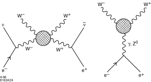
Figure 19: Processes useful for measuring the Goldstone-boson scattering amplitudes.

This theorem suggests two ways to measure amplitudes of the new strong interactions experimentally. These are illustrated schematically in Figure 19. The first is to measure the scattering of $W$ or $Z$ bosons, a process related by the theorem to the Goldstone-boson scattering amplitudes, the analogue for the new interactions of $\pi\pi$ scattering. The second is to measure the pair production of longitudinal $W$ bosons in $e^{+}e^{-}$ annihilation. This gives the analogue for the new interactions of the timelike pion form factor. In Sections 7.2 and 7.3, we will explore the application of both of these techniques at $e^{+}e^{-}$ linear colliders. We will then turn in Sections 7.4 and 7.5 to more model-dependent probes of a possible strong symmetry-breaking sector.

7.2 $WW$ Scattering at $e^{+}e^{-}$ Colliders

The scattering of $W$ bosons can be observed at high-energy colliders through processes such as $e^{+}e^{-}\to\nu\overline{\nu}+W^{+}W^{-}$ or $q\overline{q}\to q\overline{q}+WW$, as illustrated in Figure 19 [203, 204, 58]. This process has been studied in great detail in the hadronic environment; for recent reviews, see [205, 206]. For instance, the ATLAS Technical Design Report [5] includes a study showing effective rates in like-sign $W^{\pm}W^{\pm}$ scattering processes of order 20 events per LHC year, over a standard-model background of about 40 events. In some particular models of $WW$ scattering, the $WW$ invariant mass contains a resonance at some value, giving a clear signal of an effect above background. The analogous effect is seen in $\pi\pi$ scattering in QCD at the rho resonance. However, the more typical situation in parametrizations of the $WW$ scattering is that this cross section has a broad, featureless shape such as is seen in S-wave $\pi\pi$ scattering in QCD. In this situation, the effect just described for the LHC would be rather marginal, and a complementary experiment with completely different systematics would be crucial to establish the effect.

It is interesting, then, to carry out the analogous experient at an $e^{+}e^{-}$ collider, using the reactions $e^{+}e^{-}\to\nu\overline{\nu}W^{+}W^{-}$ and $e^{+}e^{-}\to\nu\overline{\nu}Z^{0}Z^{0}$ [132, 207, 208]. In the $e^{-}e^{-}$ collision mode, the reaction $e^{-}e^{-}\to\nu\nu W^{-}W^{-}$ is an equally interesting probe. The final-state $W$ and $Z$ bosons can be observed in their hadronic decay modes to maximize statistics; with the calorimeter of the JLC detector, $W$ and $Z$ bosons can be distinguished on the basis of their reconstructed masses, at least at the statistical level needed to measure the ratio of cross sections for the two processes. The size of the longitudinal $W$, $Z$ signal is order 1 fb.

The main backgrounds to the vector-boson scattering process come from the production of transversely polarized $W$, $Z$ pairs due to interactions of virtual photons radiated from the electron and positron. The most important of these are the processes $\gamma\gamma\to W^{+}W^{-}$, which has a cross section of 1–2 pb at $\sqrt{s}=1$–1.5 TeV, and from $\gamma W\to WZ$, which has a cross section of about 100 fb. These large cross sections for the background seem daunting, but the backgrounds can be removed by simple cuts. In $\gamma\gamma$ fusion, even in this case where the photons are virtual, the initial particles typically have small transverse momentum, while in $WW$ scattering the longitudinal $W$’s radiated from the electron lines typically have a transverse momentum of order $m_{W}$. Thus, it is useful to cut on the transverse momentum of the final $W$ pair, at $p_{T}(WW)>50$ GeV. The background can be decreased further by vetoing events with hard forward electrons. These two cuts remove the $\gamma\gamma$ reactions almost completely and bring the $WZ$ production to within a factor 2 of the signal [132] At this level, the calorimetric discrimination of $W$ from $Z$ reduces the $WZ$ reaction to a small background to the $WW$ and $ZZ$ signals.

Table 3: Total numbers of $W^{+}W^{-},ZZ\rightarrow 4$-jet signal $S$ and background $B$ events, after cuts, calculated for a 1.5 TeV $e^{\pm}e^{-}$ linear collider with integrated luminosity 200 fb^-1. The statistical significance $S/\sqrt{B}$ is also given. The hadronic branching fractions of $WW$ decays and a realistic $W^{\pm}/Z$ misidentification probability are included. The significance is improved by using polarized $e^{-}_{L}$ beams [208].

	SM	Scalar	Vector	LET
channels	$m_{H}=$	$M_{S}=$	$M_{V}=$
	1 TeV	1 TeV	1 TeV
$S(e^{+}e^{-}\to\overline{\nu}\nu W^{+}W^{-})$	330	320	92	62
$B$(backgrounds)	280	280	7.1	280
$S/\sqrt{B}$	20	20	35	3.7
$S(e^{+}e^{-}\to\overline{\nu}\nu ZZ)$	240	260	72	90
$B$(backgrounds)	110	110	110	110
$S/\sqrt{B}$	23	25	6.8	8.5
$S(e^{-}e^{-}_{L}\to\nu\nu W^{-}W^{-})$	54	70	72	84
$B$(background)	400	400	400	400
$S/\sqrt{B}$	2.7	3.5	3.6	4.2
$S(e^{-}_{L}e^{-}_{L}\to\nu\nu W^{-}W^{-})$	110	140	140	170
$B$(background)	710	710	710	710
$S/\sqrt{B}$	4.0	5.2	5.4	6.3

This strategy for isolating vector-boson scattering at an $e^{+}e^{-}$ collider was studied by simulation in [208]. This study did not include a realistic detector simulation but simply used the parametrization of the JLC detector. However, it did include the complete matrix elements for all relevant $2\to 4$ particle processes; for example, $\gamma\gamma\to W^{+}W^{-}$ was included as subprocess of $e^{+}e^{-}\to e^{+}e^{-}W^{+}W^{-}$. Following the framework of [205], the authors considered four particular models of the vector-boson scattering amplitude: the minimal standard model with a Higgs boson of mass 1 TeV, a model with a broad scalar resonance at 1 TeV, a model with a vector resonance at 1 TeV, and the “LET” model in which the $WW$ interactions are precisely those predicted by the low-energy theorem for pion-pion scattering, carried over to $WW$ scattering using the Equivalence Theorem. The first two of these models are rather similar. The third mimics the most naive technicolor models. The fourth is a more pessimistic scenario. The results for the signal/background estimates for these four cases, assuming a relatively high energy $\sqrt{s}=1.5$ TeV and an integrated luminosity of 200 fb^-1, are shown in Table 3. The statistical significance of the signals is comparable to that achievable at the LHC. The background estimates are presumably more solid than those made for the hadronic environment, since all important backgrounds are electroweak processes whose rates are precisely calculable. The enhancement of signal over background is improved with the use of polarized beams, as shown for $e^{-}e^{-}$ reactions in the last two lines of the Table.

It may also be possible to study $WW$ scattering at a $\gamma\gamma$ collider, by using the fact that a high-energy $\gamma$ has a large probability to branch into $W^{+}W^{-}$. One then observes the process $\gamma\gamma\to W^{+}W^{-}W^{+}W^{-}$, with two $W$’s at high transverse momentum [209, 210]

We conclude this discussion of the $WW$ scattering signal with two comments. First, while the studies we have cited for hadron and lepton colliders have considered a wide range of models of pion-pion scattering in the new strong interactions, they have all assumed that the pion-pion scattering is elastic. If the new strong sector contains other relatively light particles (so-called pseudo-Goldstone bosons), this need not be true. Then the weak vector bosons might primarily scatter into pairs of these exotic particles rather than scattering to final-state $W$ and $Z$ pairs [211]. In this case, it is extremely difficult to isolate the vector-boson scattering signal, and one must, alternatively, search for the pair production of new particles. In the hadronic environment, this could be a problem; the new particles may be recognized if they decay hadronically, especially if the dominant decays do not include top quarks. In the $e^{+}e^{-}$ environment, however, there is no difficulty in recognizing these exotic states. We will discuss search techniques for pseudo-Goldstone bosons in Section 7.4.

Second, because it is so difficult to observe the vector boson scattering signal either at hadron or electron colliders, it is important to buttress the observation of $WW$ scattering through new strong interactions by showing that there is no light Higgs particle that contributes significantly to the $W$ and $Z$ masses. We have argued in Section 5.2 that an $e^{+}e^{-}$ linear collider can discover any such light particle without relying on the assumptions of any model; conversely, it can rule out the existence of such a particle definitively. As for the LHC, though this collider can find a light Higgs boson in a large class of models, it cannot exclude the existence of such a particle except in specific model contexts.

7.3 $e^{+}e^{-}\to W^{+}W^{-}$ as a Window to Higgs Strong Interactions

In the $e^{+}e^{-}$ environment, there is a second relatively model-independent signature of new strong interactions coupling to the $W$. This is the analogue of the pion form factor in the new strong sector.

In QCD, the process $e^{+}e^{-}\to\pi^{+}\pi^{-}$ contains the rho resonance and, in fact, receives a cross section enhancement of about a factor of 20 from the resonance pole in the pion form factor. If the known strong interactions were copied at the TeV scale, the analogue of the rho in the new strong interactions would lead, through the Equivalence Theorem, to a similar enhancement in $e^{+}e^{-}\to W_{\ell}^{+}W_{\ell}^{-}$, where $W_{\ell}^{+}$ is the longitudinally polarized $W$ boson. On the other hand, we have emphasized in Section 3 that the process $e^{+}e^{-}\to W^{+}W^{-}$ is one of the major components of $e^{+}e^{-}$ annihilation at linear collider energies, and that tools exist to study this process in exquisite detail. We thus expect that effects which correspond to a percent enhancement of the rate for $W$ pair production, or a few percent enhancement of the rate of $W_{\ell}$ pair production, should be observable experimentally. This means that linear-collider experiments have a very large dynamic range in which they are sensitive to this particular amplitude arising from new strong interactions.

We will use the term “Higgs pion form factor” to refer to the form factor for the production of pairs of Goldstone bosons of the new strong interactions by the vector current of custodial $SU(2)$. If the new strong sector contains a vector meson with the $SU(2)$ quantum numbers of this current, the corresponding form factor should have a pole at the vector-boson mass, leading to a large enhancement of Goldstone-boson pair production. In a technicolor model, the new strong interactions involve new strongly interacting fermions, and the desired vector bosons appear as spin-1 $L=0$ quark-model bound states of these fermions. Vector states with these quantum numbers can also appear in other types of models, for example, models in which the constituents in the new strong interactions are vector particles [212]. One might expect more generally that, in a strongly interacting theory, the vector current should always be the interpolating field for some composite particle.

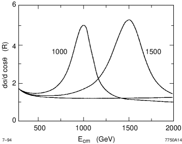
Figure 20: Effect on the unpolarized differential cross section for $e^{+}e^{-}\to W^{+}W^{-}$ at $\cos\theta=0$, plotted as a function of $E_{\hbox{\scriptsize CM}}$, of technicolor rho resonances at 1 TeV and 1.5 TeV, compared to the cross section in the minimal standard model with a light Higgs boson, from ref. [215].

In models with such strong enhancements, the effect of the vector resonance can be seen in the rate for $e^{+}e^{-}\to W^{+}W^{-}$ without any special final-state or polarization analysis [213, 214]. We should only note that the pion form factor is specifically an enhancement of longitudinal $W$ pair production. Looking back at the distributions shown in Figure 4, we see that, away from the forward peak, the longitudinal $W$ pair production accounts for about 1/4 of the differential cross section summed over polarizations. Taking into account this dilution of a factor of 4, we show in Figure 20 the effect on the differential cross section for $e^{+}e^{-}\to W^{+}W^{-}$ of a rho resonance scaled up from the familiar strong interactions to a mass of 1 TeV or 1.5 TeV [215]. A more complete analysis of production and decay distributions can observe a technirho resonance with a mass of up to 2 TeV, or exclude it at the 95% confidence level, already at $E_{\hbox{\scriptsize CM}}=500$ GeV [216].

There are, however, models with high-energy strong interactions in which there is no prominent vector resonance coupling to Goldstone-boson pairs. The minimal standard model with a heavy Higgs boson is a model of this type, and one might imagine that other models with only scalar constituents might share this property. Curiously, there is no model of this type that satisfies the criterion we set out in Section 1.1, that it explain the origin of electroweak symmetry breaking.

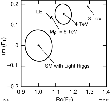
Figure 21: Confidence-level contours for the real and imaginary parts of the Higgs pion form factor $F_{\pi}$ at $\sqrt{s}=1.5$ TeV with 200 fb^-1 of data, from [70]. The simulation data was evaluated against a theory of this form factor that included both a vector resonance at a mass $M_{\rho}$ and model-independent $WW$ scattering, as described in the text. The contour about the light Higgs value is a 95% confidence contour; the contour about the point $M_{\rho}=4$ TeV is a 68% confidence contour.

Such a model can still have observable effects on the Higgs pion form factor. From unitarity and the assumption that Goldstone-boson scattering is dominantly an elastic two-body process at TeV energies, it can be shown that the vector form factor takes the form [217]

$$F_{\pi}(q^{2})=P(q^{2})\exp\left[{s\over\pi}\int ds^{\prime}{\delta_{1}(s^{\prime})\over s^{\prime}(s^{\prime}-q^{2})}\right]\ ,$$ (35)

where $\delta_{1}(s)$ is the pion-pion scattering phase shift in the channel $I=J=1$ with the quantum numbers of the vector current. The factor $P(q^{2})$ is a polynomial in $q^{2}$ such that $P(0)=1$. To obtain a concrete prediction, set $P(q^{2})=1$ [213]. In QCD, this approximation reproduces the observed pion form factor to about 20% accuracy. The phase shift $\delta_{1}$ was modelled using the prediction of the low-energy theorem for pion-pion scattering, plus a vector resonance at a specified mass. As this mass is taken to infinity, an irreducible contribution remains from $W^{+}W^{-}$ rescattering through the interactions predicted by the low-energy theorem. That contribution gave a 15% shift of the Higgs pion form factor at 1.5 TeV, mainly contributing to its imaginary part. The assumption that $P(q^{2})=1$ was questioned in [218], and the authors of that paper proposed a phenomenological model in which the polynomial has a zero in the TeV energy region. It seems difficult to resolve this controversy without reference to a plausible underlying model of the dynamics.

Nevertheless, it is interesting to see whether an enhancement of this general size can be observed experimentally. This issue was studied in [70], using the methods for the study of $e^{+}e^{-}\to W^{+}W^{-}$ that we have described in Section 3.1. Assuming a high $e^{+}e^{-}$ center-of-mass energy of 1.5 TeV and a large event sample of 200 fb^-1, comparable to what is needed for the study of $WW$ scattering, the real and imaginary parts of the Higgs pion form factor can be constrained within the limits illustrated in Figure 21. It should be noted that the sensitivity to the imaginary part of the form factor depends on the ability to make separate cross section measurements for left- and right-handed polarized beams (with 90% polarization assumed). The theoretical values of the form factor come from the model of [213], using very high values of the vector resonance mass. (The values of the vector resonance mass actually predicted in technicolor models lie far off the page to the right.) At the endpoint marked LET, the only effect is $WW$ rescattering according to the low-energy theorem. If this contribution to the the Higgs pion form factor is present in the data, the value $F_{\pi}=1$ corresponding to the minimal standard model with a light Higgs boson will be excluded at a very high level of confidence. It is remarkable that, even in this very pessimistic case, the precision study of $e^{+}e^{-}\to W^{+}W^{-}$ can provide clear evidence for the presence of new strong interactions coupling to the weak vector bosons. This window into the dynamics of the new strong sector is completely complementary to the $WW$ scattering experiments discussed in the previous section, and it is available only at $e^{+}e^{-}$ colliders.

7.4 Pseudo-Goldstone Bosons

Up to this point, we have discussed relatively model-independent signatures of a strongly coupled Higgs sector. In this section and the next, we will discuss signatures of specific models or mechanisms. Even if there is no preferred model of the new strong interactions at 1 TeV, model-dependent phenomena can be interesting to look for if they make it possible to confirm or exclude specific approaches to model-building. Signatures associated with specific mechanisms for generating the quark and lepton masses are espcially important targets for future colliders.

In Section 7.1, we discussed briefly the status of technicolor models of electroweak symmetry breaking. These models have the appealing feature that they give a clear physical explanation for the spontaneous breaking of $SU(2)\times U(1)$. However, in their simplest versions, they also have numerous phenomenological problems. It is possible to pursue the idea of technicolor by formulating more complicated models which include methods to solve these problems. We find it interesting that those mechanisms typically lead to new and distinctive experimental signatures at relatively low energies.

In technicolor models, the pseudoscalar bound states of technifermions and their antiparticles must include the Goldstone bosons which are eaten by the $W$ and $Z$ as these obtain mass. However, there may be many other such bound states. These states are massless at the level of the pure technicolor theory but receive mass from the standard model gauge couplings and other effect that break the symmetry among technifermions. Hence, they are called pseudo-Goldstone bosons. These particles typically have masses in the range of a few hundred GeV [219]. The colored bosons have larger masses than color-siglet bosons [220], giving rise to the same sort of complementarity between searches in $e^{+}e^{-}$ and $pp$ collisions that we have seen in the case of supersymmetry.

At $e^{+}e^{-}$ colliders, the search for colorless pseudo-Goldstone bosons is similar to the search for Higgs particles. Indeed, many models contain a color-singlet charged boson $P^{+}$ which decays preferentially into the heaviest fermions available. This experimental signature is identical to that of the charged Higgs boson, and is easily detected. Technicolor models often contain CP-odd bosons that decay to $\gamma\gamma$ and can therefore be produced singly in $\gamma\gamma$ collisions. The rate for this production process is similar to that for a standard Higgs boson [221]. We have explained in Section 5.4 how to discover such a particle in $\gamma\gamma$ collisions and how to measure its coupling and CP properties.

More exotic scenarios are not only possible but preferred by technicolor enthusiasts. Lane and Ramana have proposed that walking technicolor leads to “multiscale technicolor,” in which the technifermion flavor symmetry is strongly broken [222]. Then the vector mesons of the technicolor theory are not degenerate, and some of them can be quite light. The original Lane-Ramana model proposed technirho resonances at 400 and 550 GeV, though somewhat higher values may now be required. At these points, one finds resonances in $e^{+}e^{-}\to W^{+}W^{-}$ of the type discussed in Section 7.3, and also resonant enhancement of pseudo-Goldstone boson pair production.

Randall [223] and Georgi [224] have proposed solving the flavor-changing neutral current problem of technicolor by incorporating a GIM mechanism. The resulting models have a proliferation of gauge groups at 1 TeV, leading to huge multiplets of pseudo-Goldstone bosons. The phenomenology of these particles is quite complex [225].

Finally, many of the proposals for reconciling the idea of technicolor with the precision electroweak measurements depend on contributions to electroweak radiative corrections from light pseudo-Goldstone bosons [226, 227, 228] or light uncolored technifermions [229]. In either case, in order to give large electroweak corrections, the masses of these particles must be of the order of 100 GeV. The required pseudo-Goldstone bosons decay mainly to $\tau\nu_{\tau}$. They can be studied using the techniques described in Section 6.3 for the scalar $\tau$.

7.5 The Top Quark and Higgs-Sector Strong Interactions

The dynamics of fermion mass generation has the biggest effect on the property of the heaviest fermion, namely the top quark. Therefore we expect that a detailed study of the top-quark properties will give us hints about this dynamics. This is illustrated in technicolor models, for which the ETC particles that mediate the interaction between the top quark and the technifermions can be light enough to have significant effects.

In the simplest schemes for top-quark mass generation, the ETC particles are light enough to be observed in bound states with technifermions [230, 231]. These states may have masses in the range 0.5–1 TeV, and can be produced singly in association with $t$, $b$, or $\tau$. In models with topcolor [199, 201], both the composite states and the elementary top quark may exhibit couplings to the new gauge bosons of these models.

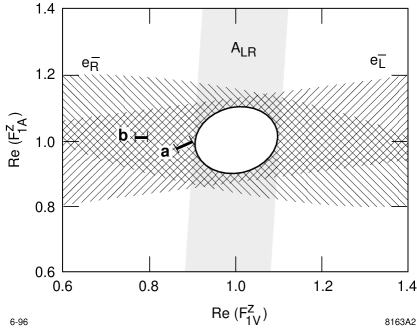
Figure 22: Expected 95% confidence limits on top-quark anomalous couplings to the $Z^{0}$, from [115], for 100 fb^-1 of data at 400 GeV in the center of mass. These bounds are compared to the expectations from the technicolor models of (a) [233] and (b) [234].

The light ETC bosons can also affect the top-quark couplings to standard-model gauge bosons. Typically, the effect of new strong interactions on the top-quark form factors of Eq. 20 is proportional to $(m_{t}/4\pi v)^{2}$, leading to effects of order 1%. However, the ETC contribution to the vector and axial-vector form factors of $t$ and $b$ turns out to contain only one power of $m_{t}$ and thus can be a 10% correction. This effect was invoked in [232] for the $b$ couplings to account for the observed anomaly in the branching ratio for $Z\to b\overline{b}$ [15]; however, in the simplest ETC model, it gives an effect of the wrong sign. More complicated ETC models can repair the sign problem and naturally give an effect on the $b$ couplings of the correct magnitude [233, 234]. These models predict similar anomalies in the top-quark couplings and thus give an idea of the size of interesting effects on these couplings from new strong dynamics. In Figure 22, we display the predictions of the models [233, 234] for the vector and axial-vector form factors in the top-quark coupling to the $Z$. These predictions are compared to the expected 95% confidence limits on these form factors, according to the simulation study of [115].

Thus, both in the study of new particles that couple to the third generation, and in the precision study of the top quark properties, $e^{+}e^{-}$ linear colliders can make significant tests of the couplings of new strong interactions to the heaviest quarks and leptons.

8 OTHER NEW PARTICLES AND INTERACTIONS

In many extensions of the standard model, there exist new particles at the TeV scale which may not necessarily be related to physics of electroweak symmetry breaking. There are numerous examples: leptoquarks, dileptons, diquarks, fourth generation, excited electrons, excited quarks, excited $W$ and $Z$ bosons, and the gauge bosons of extended gauge symmetry groups. Thanks to the democracy of the linear-collider environment, all these particles can be produced at rates comparable to the standard model backgrounds. In general, it is rather easy to discover such new particles if they are present within the kinematic reach, unless they have vanishing electroweak couplings or decay completely invisibly. Once the new particles are discovered, their standard-model quantum numbers can be worked out from their production cross sections and asymmetries, and their couplings to lighter states from their branching ratios. A recent survey of exotic particles can be found in [235]. Specific examples that have been discussed in detail include heavy neutral leptons [236], excited leptons and quarks [237], and leptoquarks [238]. We should also note that electron colliders can incisively probe into quark and lepton compositeness; for example, the study of $e^{-}e^{-}\to e^{-}e^{-}$ at 1 TeV with 50 fb^-1 of data can place a 95% confidence limit on the compositeness scale $\Lambda$ of 140 TeV [240]

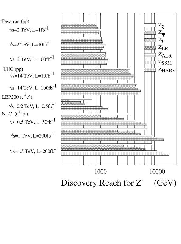
Figure 23: Comparison of the sensitivity of various colliders to $Z^{\prime}$ bosons, in seven different theoretical models, from [243]. The Tevatron and LHC bounds are based on 10 events in the $e^{+}e^{-}$ and $\mu^{+}\mu^{-}$ channels. The $e^{+}e^{-}$ collider bounds are 99% confidence limits obtained from cross sections and polarization asymmetries.

An example that deserves particular attention is the case of a new gauge boson $Z^{\prime}$ which couples to a $U(1)$ symmetry which extends the standard model gauge group. Recent surveys of the phenomenology of such bosons are given in [241, 242, 243]. Such a boson can be discovered at the LHC, as a peak in the invariant mass distribution of lepton pairs, up to a mass of several TeV. On the other hand, the few diagnostic tools available at the LHC to determine the couplings of a $Z^{\prime}$ are effective only up to about 1 TeV. A linear collider at $E_{\hbox{\scriptsize CM}}=1$ TeV would not be able to observe the resonance peak for such a heavy boson. However, it could measure the couplings of this boson to each fermion species, given the known mass value supplied by the LHC, by measuring the interference effect of the boson on forward-backward and polarization asymmetries in the fermion pair production, just as experiments at PEP, PETRA, and TRISTAN measured the couplings of fermions to the $Z^{0}$. The expected sensitivities in these two different types of measurements are shown in Figure 23. This gives a particularly clear example of the potential synergism of $e^{+}e^{-}$ and $pp$ experiments at the TeV scale.

9 CONCLUSION

In this review, we have surveyed the expected experimental program of an $e^{+}e^{-}$ linear collider operating in the energy region up to 1.5 TeV in the center of mass. We have described how this collider will be able to perform precision studies on the heaviest particles of the standard model, the $W$ boson and the top quark, and we have used these examples to demonstrate the power of $e^{+}e^{-}$ experimentation to give a concrete picture of a new physical system.

We then discussed the potential of this collider to explore new and undiscovered sectors of physics. In our arguments, we have concentrated our attention on the new physics that must be present at the TeV scale, the physics that explains the spontaneous breaking of the electroweak symmetry. We surveyed proposed models of electroweak symmetry breaking and showed that, for each case, the linear collider makes possible unique experiments that are essential for understanding the new particles and interactions that appear. We showed how the analytical tools that are available for particles of the standard model also work to illuminate states that lie outside the standard model. We considered the interplay expected in these models between the results of $e^{+}e^{-}$ and $pp$ experiments, and showed that the $e^{+}e^{-}$ experiments typically supply crucial ingredients needed to interpret signals seen in the hadronic environment.

We do not know what physics is waiting for us at the next step in energy. That is the puzzle that we must solve. We have argued here that $e^{+}e^{-}$ linear colliders are well matched to this task and will play a central role in this solution.

ACKNOWLEDGEMENTS

We thank many friends at KEK, LBL, and SLAC, and in the broader community, who have educated us on the issues we have discussed here. We are particularly grateful to Tim Barklow, David Burke, Keisuke Fujii, Howard Haber, Kaoru Hagiwara, Ken-ichi Hikasa, Gordon Kane, Akiya Miyamoto, and Peter Zerwas, who have influenced our perspective through many years of arguments and conversations. This work was supported by the National Science Foundation under grant PHY-90-21139 and by the Department of Energy under contracts DE-AC03-76SF00098 and DE–AC03–76SF00515.

References

- [1] LHC Study Group. The Large Hadron Collider: Conceptual Design. CERN/AC/95-05 (LHC) (1995)
- [2] Chanowitz MS. Ann. Rev. Nucl. Part. Sci. 38:323 (1988)
- [3] Ellis N and Virdee TS. Ann. Rev. Nucl. Part. Sci. 44:609 (1994)
- [4] CMS Collaboration. Technical Proposal. CERN/LHCC/94-38 (1994)
- [5] ATLAS Collaboration. Technical Proposal. CERN/LHCC/94-43 (1994)
- [6] Eichten E, Hinchliffe I, Lane K, and Quigg C. Rev. Mod. Phys. 56:579 (1984), 58:1073 E (1986)
- [7] Orava, R, Eerola P, and Nordberg M, eds. Physics and Experiments with Linear Colliders. (World Scientific, Singapore, 1992)
- [8] Harris FA, Olsen SL, Pakvasa S, and Tata X, eds. Physics and Experiments with Linear Colliders. (World Scientific, Singapore, 1993)
- [9] Miyamoto A and Fujii Y, eds. Physics and Experiments with Linear Colliders. (World Scientific, Singapore, 1996)
- [10] Zerwas PM, ed. Collisions at 500 GeV: The Physics Potential, vols. A, B. DESY report DESY-92-123 (1992)
- [11] Zerwas PM, ed. Collisions at 500 GeV: The Physics Potential, vol. C. DESY report DESY-93-123C (1993)
- [12] Barklow TL, Haber HE, Dawson S, and Siegrist JL, eds. Electroweak Symmetry Breaking and New Physics at the TeV Scale. (World Scientific, Singapore, 1996)
- [13] Glashow SL. Nucl. Phys. 22:579 (1961); Weinberg S. Phys. Rev. Lett. 19:1264 (1967); Salam A. in Elementary Particle Theory, N Svartholm, ed. (Wiley, New York, 1968)
- [14] Langacker P and Erler J. in Review of Particle Properties, Phys. Rev. D50:1173 (1994)
- [15] Hagiwara K. preprint hep-ph/9512425, to appear in the proceedings of the International Symposium on Lepton Photon Interactions, Beijing, 1995
- [16] Bjorken JD and Weinberg S. Phys. Rev. Lett. 38:622 (1977); Bjorken JD, Lane K, and Weinberg S, Phys. Rev. D16:1474 (1977)
- [17] Eichten E and Lane K. Phys. Lett. 90B:125 (1980)
- [18] Barbieri R and Hall LJ. Phys. Lett. B338:212 (1994)
- [19] Mulvey JH, ed. Proceedings of Workshop on Physics at Future Accelerators. CERN-87-07 (1987)
- [20] Ahn C et al.Opportunities and Requirements for Experimentation at a Very High-Energy Collider, SLAC-Report-329 (1988)
- [21] Kawabata S, ed. Proceedings of the Second JLC Workshop. KEK-Proceedings-91-10 (1991)
- [22] Palmer RB. Ann. Rev. Nucl. Part. Sci. 40:529 (1990)
- [23] Settles R, ed. Proceedings of the ECFA Workshop on Linear Colliders (LC92). (Max Planck Institute, Munich, 1993)
- [24] Asher K and Paterson JM, eds. Proceedings of the Fifth International Workshop on Linear Colliders (LC93). SLAC-Report-436 (1994)
- [25] Urakawa J, ed. Proceedings of the Sixth International Workshop on Linear Colliders (LC95). KEK Proceedings 95-5 (1995)
- [26] Loew G et al.International Linear Collider Technical Review Committee Report 1995. SLAC report SLAC-R-95-471
- [27] Chen P. unpublished technical note for the study [26]
- [28] Wilson PB. in Proceedings of the 1986 Linear Accelerator Conference, SLAC report SLAC-303 (1986)
- [29] Himel T and Siegrist J. SLAC preprint SLAC-PUB-3572 (1985)
- [30] Noble RJ. NIM A256:427 (1987)
- [31] Chen P and Telnov V. Phys. Rev. Lett. 63:1796 (1989)
- [32] NLC ZDR Design Group. Zeroth Order Design Report for the Next Linear Collider. SLAC-Report-474 (1996)
- [33] NLC ZDR Design Group and NLC Physics Working Groups. Physics and Technology of the Next Linear Collider. BNL 52-502, FERMILAB-PUB-96/112, LBNL-PUB-5425, SLAC-Report-485, UCRL-ID-124160, UC-414 (1996)
- [34] Seeman JT. Ann. Rev. Nucl. Part. Sci. 41:389 (1991)
- [35] Decamp D et al.(ALEPH Collaboration). Phys. Repts. 216:253 (1992)
- [36] Miyamoto A. in [8]
- [37] Drees M and Godbole RM. Phys. Rev. Lett. 67:1189 (1991)
- [38] Forshaw JR and Storrow JK. Phys. Lett. B278:193 (1992)
- [39] Chen P, Barklow TL, and Peskin ME. Phys. Rev. D49:3209 (1994)
- [40] Decamp D et al.(ALEPH Collaboration). NIM A294:121 (1990), A303:393 E (1991)
- [41] SLD Collaboration. SLD Design Report. SLAC-Report-273 (1984)
- [42] JLC Group. JLC-I. KEK-Report 92-16 (1992)
- [43] Miyamoto A. in Proceedings of the Second JLC Workshop, S Kawabata, ed. KEK-Proceedings-91-10 (1991)
- [44] Frary MN and Miller DJ. in [10]
- [45] Montague BW. Phys. Repts. 113:1 (1984)
- [46] Maruyama T et al.Phys. Rev. Lett. 66:2376 (1991), Phys. Rev. B46:4261 (1992)
- [47] Omori T, et al.Phys. Rev. Lett. 67:3294 (1991); Nakanishi T et al., Phys. Lett. A158:345 (1991)
- [48] Mikhailichenko AA. in Proceedings of the International Workshop on Sources and Pre-Accelerators for Linear Colliders, R Wanzenberg, ed. (DESY, 1994)
- [49] Heusch CA, ed. Proceedings of the Electron-Electron Linear Collider Workshop, Int. J. Mod. Phys. A11:1523 (1996)
- [50] Ginzburg IF, Kotkin GL, Serbo VG, and Telnov VI. JETP Lett. 34:491 (1982), NIM 205:47 (1983); Ginzburg IF, Kotkin GL, Panfil SL, Serbo VG, and Telnov VI. NIM 219:5 (1984)
- [51] Telnov VI. NIM A294:72 (1990)
- [52] Heinrich JG et al.SLAC Proposal E-144 (1991)
- [53] Borden DL, Bauer DA, and Caldwell DO. Phys. Rev. D48: 4018 (1993)
- [54] K Hagiwara K, Peccei RD, Zeppenfeld D, and Hikasa K. Nucl. Phys. B282:253 (1987)
- [55] Cornwall JM, Levin DN, and Tiktopoulos G. Phys. Rev. D10:1145 (1974)
- [56] Vayonakis CE. Lett. Nuov. Cim. 17:383 (1976)
- [57] Lee BW, Quigg C, and Thacker HB. Phys. Rev. Lett. 38:883 (1977), Phys. Rev. D16:1519 (1977)
- [58] Chanowitz MS and Gaillard MK. Nucl. Phys. B261:379 (1985)
- [59] Bohm M, Denner A, Sack T, Beenacker W, Behrends F, and Kuijf H. Nucl. Phys. B304:463 (1988); Beenacker W, Denner A, Dittmaier S, Mertig R, and Sack T. Nucl. Phys. B410:245 (1993); Beenacker W et al.CERN report CERN-96-01
- [60] Dawson S and Valencia G. Phys. Rev. D49:2188 (1994).
- [61] Holdom B. Phys. Lett. B258:156 (1991)
- [62] Einhorn M and Wudka J. in Proceedings of the International Workshop on Electroweak Symmetry Breaking, T Muta, ed. (World Scientific, Singapore, 1992); M. Einhorn, in [8]
- [63] De Rujula A, Gavela MB, Hernandez P, and Masso E. Nucl. Phys. B384:3 (1992)
- [64] Burgess CP and London D. Phys. Rev. Lett. 69:3428 (1992), Phys. Rev. D48:4337 (1993)
- [65] Appelquist T and Wu GH. Phys. Rev. D51:240 (1995)
- [66] Gasser J and Leutwyler H. Nucl. Phys. B250:465 (1985)
- [67] Peskin ME and Takeuchi T. Phys. Rev. Lett. 65:964 (1990); Phys. Rev. D46:381 (1992)
- [68] Barklow T. in [7]
- [69] Frank M, Mättig P, Settles R, and Zeuner W. in [10]
- [70] Barklow T. in The Albuquerque Meeting, Proceedings of the 1994 DPF Meeting, S Seidel, ed. (World Scientific, Singapore, 1995)
- [71] Aihara H et al.in [12].
- [72] Hagiwara K, Ishihara S, Szalapski R, and Zeppenfeld D. Phy. Lett. B283:353 (1992)
- [73] Yehudai E. Phys. Rev. D41:33 (1990)
- [74] Yehudai E. Phys. Rev. D44:3434 (1991)
- [75] Choi SY and Schrempp R. Phys. Lett. B272:149 (1991)
- [76] Brodsky SJ, Rizzo TG, and Schmidt I. Phys. Rev. D52:4929 (1995)
- [77] Bèlanger G and Boudjema F. Phys. Lett. B288:201,210 (1992)
- [78] Jezabek M and Kühn JH. Nucl. Phys. B314:1 (1989)
- [79] Jezabek M and Kühn JH. Phys. Rev. D48:1910 (1993), D49:4970 E (1994)
- [80] Bigi I and Krasemann H. Z. Phys. C7:127 (1981)
- [81] Kühn JH. Acta Phys. Austr. Suppl. XXIV:230 (1982)
- [82] Bigi I, Dokshitser Yu, Khoze V, Kühn J, and Zerwas P. Phys. Lett. 181B:157 (1986)
- [83] Fadin VS and Khoze VA. JETP Lett. 46:525 (1987), Sov. J. Nucl. Phys. 48:309 (1988)
- [84] Kwong W. Phys. Rev. D43:1488 (1991)
- [85] Strassler MJ and Peskin ME. Phys. Rev. D43:1500 (1991)
- [86] Komamiya S. in Research Directions for the Decade: Snowmass ’90, EL Berger, ed. (World Scientific, Singapore, 1992)
- [87] Igo-Kemenes P, Martinez M, Miquel M, and Orteu S. in [11]
- [88] Fujii K, Matsui T, and Sumino Y. Phys. Rev. D50:4341 (1994); Sumino Y. Acta. Phys. Polon. 25:1837 (1994)
- [89] Comas P, Miquel R, Martinez M, and Orteu S. preprint CERN-PPE/96-40 (1996)
- [90] Amidei D and Brock R, eds. Future ElectroWeak Physics at the Fermilab Tevatron, FERMILAB-PUB-96/046 (1996)
- [91] Manohar A. in Review of Particle Properties, Phys. Rev. D50:1173 (1994)
- [92] Gray N, Broadhurst DJ, Grafe W, and Schilcher K. Z. Phys. C48:673 (1990)
- [93] Sumino Y. Ph. D. thesis, preprint UT-655 (1993)
- [94] Sumino Y, Fujii K, Hagiwara K, Murayama H, and Ng CK. Phys. Rev. D47:56 (1992)
- [95] Jezabek M and Teubner T. Z. Phys. C59:669 (1993)
- [96] Kummer W and Modritsch W. Phys. Lett. B349:525 (1995)
- [97] Jezabek M, Kühn JH, and Teubner T. Z. Phys. C56:653 (1992)
- [98] Murayama H and Sumino Y. Phys. Rev. D47:82 (1992)
- [99] Venturi A. in [11]
- [100] Yuan CP. Phys. Rev. D41:42 (1990); Carlson DO and Yuan CP. Phys. Lett. B306:390 (1993)
- [101] Stelzer T and Willenbrock S. Phys. Lett. B357:125 (1995)
- [102] Feigenbaum J. Phys. Rev. D43:264 (1991)
- [103] Jezabek M and Kühn JH. Phys. Lett. B316:360 (1993); Harlander R, Jezabek M, and Kühn JH. preprint hep-ph/9506292
- [104] Jersak J, Laermann E, and Zerwas PM. Phys. Rev. D25:1218 (1982), D36;310 E (1987)
- [105] Czarnecki A, Jezabek M, and Kühn JH. Nucl. Phys. B351:70 (1991)
- [106] Kane GL, Ladinsky GA, Yuan CP. Phys. Rev. D45:124 (1992)
- [107] Dokhshitzer YuL, Khoze VA, and Stirling WJ. Nucl. Phys. B428:3 (1994); Orr LH, Stelzer T, and Stirling WJ. Phys. Lett. B354, 442 (1995); Ballestrero A, Khoze VA, Maina E, Moretti S, and Stirling WJ. preprint hep-ph/9511308
- [108] Schmidt CR. preprint hep-ph/9504434
- [109] Yuan CP. Phys. Rev. D45:782 (1992)
- [110] Atwood D and Soni A. Phys. Rev. D45:2405 (1992)
- [111] Atwood D, Eilam G, Soni A, Mendel RR, Migneron R. Phys. Rev. Lett. 70:1364 (1993); Atwood D, Eilam G, and Soni A. Phys. Rev. Lett. 71:492 (1993)
- [112] Bernreuther W, Nachtmann O, Overmann P, and Schroder T. Nucl. Phys. B388:53 (1992), B406:516 E (1993); Anlauf H, Bernreuther W, and Brandenberg A. Phys. Rev. D52:3803 (1995), D53:1725 E (1996)
- [113] Bar-Shalom S, Atwood D, Eilam G, Mendel RR, and Soni A. Phys. Rev. D53:1162 (1996)
- [114] Ladinsky GA and Yuan CP. Phys. Rev. D49:4415 (1994); Carlson DO, Malkawi E, and Yuan CP. Phys. Lett. B337:145 (1994)
- [115] Barklow TL and Schmidt CR. in The Albuquerque Meeting, Proceedings of the 1994 DPF Meeting, S Seidel, ed. (World Scientific, Singapore, 1995)
- [116] Frey R. in [9]
- [117] Harlander R, Jezabek M, Kühn JH, and Teubner T. Phys. Lett. B346:137 (1995); Harlander R, Jezabek M, Kühn JH, and Peter M. preprint hep-ph/9604328
- [118] Parke S and Shadmi Y. preprint FERMILAB-PUB-96/042-T (1996)
- [119] Grivaz JF. preprint LAL-95-83 (1995), to appear in the proceedings of the International Europhysics conference on High Energy Physics, Brussels, 1995
- [120] Heller UM, Klomfass M, Neuberger H, and Vranas P. Nucl. Phys. B405:555 (1993)
- [121] Okada Y, Yamaguchi M, and Yanagida T. Prog. Theor. Phys. 85:1 (1991)
- [122] Haber HE and Hempfling R. Phys. Rev. Lett 66:1815 (1991)
- [123] Ellis J, Ridolfi G, and Zwirner F. Phys. Lett. B257:83 (1991)
- [124] Cabibbo N, Maiani L, Parisi G, Petronzio R. Nucl. Phys. B158:295 (1979)
- [125] Sher M. Phys. Repts. 179:273 (1989)
- [126] Drees M. Int. J. Mod. Phys. A4:3635 (1989)
- [127] Moroi T and Okada Y. Mod. Phys. Lett. A7:187 (1992); Phys. Lett. B295:73 (1992)
- [128] Kane GL, Kolda C, and Wells JD. Phys. Rev. Lett. 70:2686 (1993)
- [129] Gunion JF, Haber HE, Kane GL, and Dawson S. The Higgs Hunter’s Guide. (Addison-Wesley, Redwood City, 1990)
- [130] Gunion J, Stange A, and Willenbrock S. in [12]
- [131] Barger V, Cheung K, Kniehl BA, and Phillips RJN. Phys. Rev. D46:3725 (1992)
- [132] Hagiwara K, Kanzaki J, and Murayama H. preprint KEK-TH-282 (1991)
- [133] Kurihara Y. in Proceedings of the Second Workshop on Japan Linear Collider, S Kawabata, ed. (KEK, 1990)
- [134] Janot P. in [8]
- [135] Barger V, Cheung K, Djouadi A, Kniehl BA, and Zerwas PM. Phys. Rev. D49:79 (1994)
- [136] Gunion JF, et al.Phys. Rev. D38:3444 (1988)
- [137] Eerola P and Sirkka J. in [10]
- [138] Sopczak A. in [11]
- [139] Gunion JF and Haber HE. Nucl. Phys. B272:1 (1986), B278:449 (1986), B307:445 (1988)
- [140] Djouadi A, Kalinowski J, and Zerwas PM. Z. Phys. C57:569 (1993)
- [141] Hildreth MD, Barklow TL, and Burke DL. Phys. Rev. D49:3441 (1994)
- [142] Keung WY and Marciano WJ. Phys. Rev. D30:248 (1984)
- [143] Bartel W et al.Z. Phys. C33:23 (1986)
- [144] Nakamura I. in [9]; Nakamura I and Kawagoe K. preprint hep-ex/9604010
- [145] Djouadi A, Kalinowski J, and Zerwas PM. Z. Phys. C54:255 (1992), Mod. Phys. Lett. A7:1765 (1992)
- [146] Gunion JF and Haber HE. Phys. Rev. D48:5109 (1993)
- [147] Eboli OJP, Gonzalez-Garcia MC, Halzen F, and Zeppenfeld D. Phys. Rev. D48:1430 (1993)
- [148] Borden DL, Khoze VA, Stirling WJ, and Ohnemus J. Phys. Rev. D50:4499 (1994)
- [149] Jikia G. and Tkabladze A. preprint hep-ph/9406428
- [150] Watanabe I. preprint hep-ph/9504226
- [151] Jikia G and Tkabladze A. preprint hep-ph/9601384
- [152] Jikia G. Phys. Lett. B298:224 (1993), Nucl. Phys. B405:24 (1993)
- [153] Kane GL, Kribs GD, Martin SP, and Wells JD. Phys. Rev. D53:213 (1996)
- [154] Gunion JF, Kelly JG, and Ohnemus J. Phys. Rev. D51:2101 (1995)
- [155] Grzadkowski B and Gunion JF. Phys. Lett. B294:361 (1992)
- [156] Kramer M, Kühn JH, Stong ML, and Zerwas PM. Z. Phys. C64:21 (1994)
- [157] Weinberg S. Phys. Rev. D42:860 (1990)
- [158] Nilles HP. Phys. Repts. 110:1 (1984)
- [159] Haber HE and Kane GL. it Phys. Repts. 117:75 (1985)
- [160] Haber HE. in Recent Directions in Particle Theory (TASI-92), J Harvey and J Polchinski, eds. (World Scientific, Singapore, 1993)
- [161] Murayama H. in Physics with High Energy Colliders, S Yamada and T Ishii, eds. (World Scientific, Singapore, 1995)
- [162] Bagger JA. preprint hep-ph/9604232, to appear in the proceedings of TASI-95
- [163] Langacker P and Polonsky N. Phys. Rev. D47:4028 (1993), Phys. Rev. D52, 3081 (1995)
- [164] Ibanez LE and Ross GG. in Perspectives in Higgs Physics, GL Kane, ed. (World Scientific, Singapore, 1993)
- [165] Ellis J, Enqvist K, Nanopoulos DV, and Zwirner F. Mod. Phys. Lett. A1:57 (1986)
- [166] Barbieri R and Giudice GF. Nucl. Phys. B306:63 (1988)
- [167] Anderson GW and Castaño DJ. Phys. Rev. D52:1693 (1995), Phys. Rev. D53:2403 (1996)
- [168] Baer H, Chen CH, Paige F, and Tata X. Phys. Rev. D49:3283 (1994), D53:6241 (1996)
- [169] Baer H, Chen CH, Paige F, and Tata X. Phys. Rev. D52:2746 (1995)
- [170] Baer H et al.in [12]
- [171] Dimopoulos S and Hall L. Phys. Lett B207:210 (1988)
- [172] Dreiner H and Ross GG. Nucl. Phys. B365:597 (1991)
- [173] Baer H, Bartl A, Karatas D, Majerotto W, and Tata X. Int. J. Mod. Phys. A4:4111 (1989); Bartl A, Majerotto W, and Mösslacher B. in [10]
- [174] Grivaz JF, in [7].
- [175] Tsukamoto T, Fujii K, Murayama H, Yamaguchi M, and Okada Y. Phys. Rev. D51:3153 (1995)
- [176] Feng JL, Peskin ME, Murayama H, and Tata X. Phys. Rev. D52:1418 (1995)
- [177] Becker R and Van der Velde C. in [11]
- [178] Cuypers F, van Oldenborgh GJ, and Rückl R. Nucl. Phys. B409:128 (1993)
- [179] Arkani-Hamed N, Cheng HC, Feng JL, and Hall LJ. preprint hep-ph/9603431
- [180] Kon T. it Phys. Lett. B316:181 (1993); Cuypers F, van Oldenborgh GJ, and Rückl R. Nucl. Phys. B409:144 (1993); Goto A and Kon T. Europhys. Lett. 13:211 (1990), 14:281 E (1991)
- [181] Nojiri MM. Phys. Rev. D51:6281 (1995); Fujii K, Tsukamoto T, and Nojiri MM. in [9]
- [182] Feng JL and Finnell DE. Phys. Rev. D49:2369 (1994)
- [183] Bartl A, Eberl H, Kraml S, Majerotto W, Porod W, and Sopczak A. preprint hep-ph/9604221
- [184] Peskin ME. preprint hep-ph/9604339, to appear in the proceedings of the Yukawa International Symposium, 1995, T Kugo, ed.
- [185] Barnett M, Gunion JF, and Haber HE. Phys. Lett. B315:349 (1993)
- [186] Baer H, Barger V, Karatas D, and Tata X. Phys. Rev. D36:96 (1987); Baer H, Tata X, and Woodside J. Phys. Rev. D42:1568 (1990), D45:142 (1992)
- [187] Barnett RM, Gunion JF, and Haber HE. Phys. Rev. D37:1892 (1988)
- [188] Higgs PW. Phys. Rev. Lett. 13:508 (1964)
- [189] Weinberg S. Phys. Rev. D19: 1277 (1979)
- [190] Susskind L. Phys. Rev. D20:2619 (1979)
- [191] Eichten E, Lane K, and Preskill J. Phys. Rev. Lett. 45:225 (1980)
- [192] Dimopoulos S and Ellis J. Nucl. Phys. B182:505 (1982)
- [193] Raby S. Nucl. Phys. B187:446 (1981)
- [194] Holdom B. Phys. Rev. D24:1441 (1981)
- [195] Appelquist TW, Karabali D, and Wijewardhana LCR. Phys. Rev. Lett. 57:957 (1986)
- [196] Nambu Y. in Proceedings of the 1989 Workshop on Dynamical Symmetry Breaking, T Muta and K Yamawaki, eds. (Nagoya University, 1990)
- [197] Miranskii VA, Tanabashi M, and Yamawaki K. Phys. Lett. B221:177 (1989), Mod. Phys. Lett. A4:1043 (1989)
- [198] Bardeen WA, Hill CT, and Lindner M. Phys. Rev. D41:1647 (1990)
- [199] Hill CT. Phys. Lett. B266:419 (1991)
- [200] Chivukula RS, Cohen AG, and Lane K. Nucl. Phys. B343:554 (1990)
- [201] Hill CT. Phys. Lett. B345:483 (1995); Lane K and Eichten E, Phys. Lett. B352:382 (1995)
- [202] Sikivie P, Susskind L, Voloshin M, and Zakharov V. Nucl. Phys. B173:189 (1980)
- [203] Jones DRT and Petkov S. Phys. Lett. B84:440 (1979)
- [204] Cahn RN and Dawson S. Phys. Lett. B136:196 (1984)
- [205] Bagger J, Barger V, Cheung K, Gunion J, Han T, Ladinsky GA, Rosenfeld R, and Yuan CP. Phys. Rev. D49:1246 (1994), D52:3878 (1995)
- [206] Chivukula RS, Dugan MJ, Golden M, and Simmons EH. Ann. Rev. Nuc. Part. Sci. 45:255 (1995)
- [207] Kurihara Y and Najima R. Phys. Lett. B301:292 (1993); Kurihara Y and Najima R. in Proceedings of the Fourth Workshop on JLC. KEK Proceedings 94-01 (1994)
- [208] Barger V, Cheung K, Han T, Phillips RJN. Phys. Rev. D52:3815 (1995)
- [209] Brodsky SJ. in [8]
- [210] Cheung K. Phys. Lett. B323:85 (1994)
- [211] Chivukula RS and Golden M. Phys. Lett. B267:233 (1991); Chivukula RS, Golden M, and Ramana MV. Phys. Lett. B293:400 (1992)
- [212] Veltman M. Phys. Lett. B139:307 (1984); Veltman H and Veltman M. Acta Phys. Polon. B22:669 (1991)
- [213] Peskin ME. in Physics in Collision 4, A. Seiden, ed. (Editions Frontieres, Gif-sur-Yvette, 1984)
- [214] Iddir F, Le Yaouanc A, Oliver L, Pene O, and Raynal JC. Phys. Rev. D41:22 (1990)
- [215] Peskin ME. in [7]
- [216] Miyamoto A, Hikasa KI, and Izubuchi T. in Proceedings of the INS Workshop on the Physics of , , and Collisions, Z Hioki, T Ishii, and R Najima, eds. (INS, Tokyo, 1995)
- [217] Bjorken JD and Drell SD. Relativistic Quantum Fields, Ch. 18.13. (McGraw-Hill, New York, 1965)
- [218] Basdevant JL, Berger EL, Dicus D, Kao C, and Willenbrock S. Phys. Lett. B313: 402 (1993)
- [219] Chivukula RS, Rosenfeld R, Simmons EH, and Terning J. in [12]
- [220] Peskin ME. Nucl. Phys. B175: 197 (1980), Preskill JP. Nucl. Phys. B177:221 (1981)
- [221] Tandean J. Phys. Rev. D52:1398 (1995)
- [222] Lane K and Ramana MV. Phys. Rev. D44:2678 (1991); Eichten E and Lane K. Phys. Lett. B327:129 (1994)
- [223] Randall L. Nucl. Phys. B403:122 (1993)
- [224] Georgi H. Nucl. Phys. B416:699 (1994)
- [225] Skiba W. preprint hep-ph/9601217
- [226] Dugan MJ and Randall L. Phys. Lett. B264:154 (1991)
- [227] Sundrum R and Hsu S. Nucl. Phys. B391:127 (1993)
- [228] Luty M and Sundrum R. preprint hep-ph/9209255
- [229] Gates E and Terning J. Phys. Rev. Lett. 67:1840 (1991); Appelquist T and Terning J. Phys. Lett. B315:139 (1993)
- [230] Arnold P and Wendt C. Phys. Rev. D33:1873 (1986)
- [231] Appelquist T and Evans N. Phys. Rev. D53:2789 (1996)
- [232] Chivukula RS, Selipsky SB, and Simmons EH. Phys. Rev. Lett. 69:575 (1992)
- [233] Chivukula RS, Simmons EH, and Terning J. Phys. Lett. B331:383 (1994)
- [234] Hagiwara K and Kitazawa N. Phys. Rev. D52:5374 (1995)
- [235] Djouadi A, Ng J, and Rizzo T. in [12]; Azuelos G and Djouadi A. Z. Phys. C63:317, 327 (1994)
- [236] Buchmüller W, Greub C, Minkowski P, Talby M, and Tysarczyk-Niemeyer G. in [10]; Buchmüller W and Greub C. Nucl. Phys. B363:345 (1991), B381:109 (1992)
- [237] Boudjema F, Djouadi A, and Kneur JL. Z. Phys. C57:425 (1993)
- [238] Nadeau H and London D. Phys. Rev. D47:3742 (1993); Bèlanger G, London D, and Nadeau H. Phys. Rev. D49:3140 (1994)
- [239] Doncheski MA and Godfrey S. Phys. Rev. D51:1040 (1995)
- [240] Barklow T. Int. J. Mod. Phys. A11:1579 (1996)
- [241] Hewett JL. in [8]
- [242] Del Aguila F, and Cvetic M. Phys. Rev. D50:3158 (1994); Del Aguila F, Cvetic M, and Langacker P. Phys. Rev. D52:37 (1995)
- [243] Cvetic M and Godfrey S. in [12]