Abstract

Once a light Higgs boson is discovered at a future ${\rm e}^{+}{\rm e}^{-}$ collider, the next target at the collider will be precise measurements of the Higgs boson properties. In this paper we report a simulation study on the measurement of the ratio $Br(H\to c\bar{c},gg)/Br(H\to b\bar{b})$ at center of mass energy of 300 GeV, and show the possibility to constrain MSSM parameters from the measurement.

( To appear in Physical Review D)

1 Introduction

Next generation ${\rm e}^{+}{\rm e}^{-}$ linear colliders, firstly to be operated at center of mass energies ($\sqrt{s}$ ) of 300-500 GeV (phase 1) and to be then upgraded to 1 TeV or higher (phase 2), have been proposed by several groups in recent years [1, 2, 3, 4, 5]. At the first phase of such colliders the main target is the Higgs boson, the only undiscovered participant in the Standard Model (SM). According to the recent precision electroweak measurements at LEP and SLC, Supersymmetry (SUSY) has become more favorable. In the Minimal Supersymmetric extension of the Standard Model (MSSM), two Higgs doublets are necessary to give the masses of up and down type fermions. Two neutral scalars ($h^{0},H^{0}$), a pseudoscalar ($A^{0}$) and a pair of charged Higgs ($H^{\pm}$) are introduced in this extended Higgs sector. The mass of the lightest neutral Higgs ($m_{h^{0}}$) is smaller than that of the $Z^{0}$ boson ($m_{Z^{0}}$) at tree level. Even if radiative corrections are taken into account, $m_{h^{0}}$ is at most $\sim$ 130 GeV for a top mass ($m_{t}$) of 170 GeV [6, 7, 8]. This situation does not change significantly in extended SUSY models [9]. Therefore if SUSY is correct, discovery of at least one neutral Higgs boson is guaranteed at the first phase.

After having discovered the Higgs boson, the next step is to distinguish whether the Higgs is SM-like or SUSY-like. This can be done by measuring the ratio of branching fractions $Br(H\to c\bar{c})/Br(H\to b\bar{b})$ or almost equivalently $Br(H\to c\bar{c},gg)/Br(H\to b\bar{b})$. In the MSSM these values are smaller than those of the SM. As the value $Br(H\to c\bar{c})/Br(H\to b\bar{b})$ (or $Br(H\to c\bar{c},gg)/Br(H\to b\bar{b})$) has a strong correlation to the $A^{0}$ mass ($m_{A^{0}}$) and almost independent from the SUSY energy scale ($m_{\rm SUSY}$), it is pointed out that a constraint on $m_{A^{0}}$ can be obtained from this measurement [10]. Fig. 1 shows the relation between $Br(H\to c\bar{c},gg)/Br(H\to b\bar{b})$ and $m_{A^{0}}$.

Relation between $Br(H\to c\bar{c},gg)/Br(H\to b\bar{b})$ and $m_{A^{0}}$  [10].

The mass of the bottom quark ($m_{b}$) is important in this relation, since the ratio $Br(H\to c\bar{c},gg)/Br(H\to b\bar{b})$ is proportional to $m_{b}^{-2}$. We can use the measurement of $Br(H\to{\tau}^{+}{\tau}^{-})$ to determine $m_{b}$, through the relation $Br(H\to{\tau}^{+}{\tau}^{-})/Br(H\to b\bar{b})\propto m_{\tau}^{2}/m_{b}^{2}$ which is valid both in the SM and SUSY models.

The total production cross section of the process $e^{+}e^{-}\to HZ^{0}$ ($\sigma_{tot}$) can be determined by counting the events, in which the $Z^{0}$ decays into a pair of leptons whose recoil mass is consistent with the Higgs mass. This technique is valid even if $H$ has decay channels to undetectable particles such as neutralinos, since only the $Z^{0}$ decay products are used in the event selection.

A previous simulation study for the measurement of the Higgs boson branching fractions can be found in Ref. [11], where the measurement was studied at $\sqrt{s}=$ 400-500 GeV mainly for $m_{H}=140$ GeV. The authors of Ref. [11] claimed that the statistical error of the $Br(H\to c\bar{c},gg)/Br(H\to b\bar{b})$ measurement would be about 40 % for the 120 GeV Higgs with an integrated luminosity of 50 fb^-1. However, their result is not sufficient to provide strong constraints on $m_{A^{0}}$, and the Higgs mass of 140 GeV may be too heavy if we assume the MSSM. Therefore we perform here an extended simulation study focusing on the measurement of the ratio $Br(H\to c\bar{c},gg)/Br(H\to b\bar{b})$ assuming a SM-like Higgs, where we try to improve the measurement as follows;

• setting $\sqrt{s}=$300 GeV to avoid large background from top pair productions

• using all the $Z^{0}$ decay modes to reduce statistical errors

• studying the effect of beam polarization to reduce electroweak background.

2 Event Generation and Detector Simulation

We use Pythia5.7 + Jetset7.4 [12] to calculate the cross sections and to generate events of the processes $e^{+}e^{-}\to Z^{0}H$ and major background processes. We use the quark masses of $m_{t}=$ 170 GeV, $m_{b}=$ 4.25 GeV and $m_{c}=$ 1.35 GeV and initial state radiations are considered. A cross check using GRACE 1.1 [13] shows no inconsistency in cross sections and angular distributions. Table 1 shows the list of branching ratios, cross sections and expected number of events in a year (50 fb^-1) for the SM Higgs boson. Number of generated events both for signal and background processes in this study are also listed. The cross sections with 90 % polarized electron beam are obtained from the cross sections and angular distributions calculated with GRACE 1.1.

The 4-momenta of all decay products given by the event generator are fed into a fast detector simulation program which is based on a smearing method with the standard parameters of the JLC-I Detector given in Ref. [1]. The characteristics of the detector simulator are the following:

• A pixel type vertex detector (VTX) with a pixel size of $25\times 25\mu m^{2}$ is assumed.

• The momentum resolution of the central drift chamber (CDC) is assumed to be $\sigma_{p_{t}}/p_{t}=1.1\times 10^{-4}\cdot p_{t}\oplus 0.1\%$ ($p_{t}$ in GeV).

• The electromagnetic and hadronic calorimeter hits are created according to the energy resolutions of $15\%/\sqrt{E}\oplus 1\%$ and $40\%/\sqrt{E}\oplus 2\%$, respectively ($E$ in GeV).

• The momentum measured with the CDC is always used for a charged track rather than the energy measured with the calorimeter.

• The contribution of charged tracks is subtracted from the energy of the calorimeter clusters in order to extract the energy of neutral particles.

• All electrons(muons) with momentum above 1 GeV(2 GeV) are assumed to be perfectly identified.

Table 1: Branching ratios, cross sections, expected numbers of events, expected numbers of events with 90 % polarized electron beam and numbers of generated signal and background events in a year for the SM Higgs boson with a mass of 120 GeV (50 fb^-1). Cross sections for $e^{+}e^{-}\to e\nu W,e^{+}e^{-}Z^{0}$ with 90 % polarized electron beam are not calculated here since no events survived the selection criteria described in section 3.

$m_{H}$=120 GeV	Br (%)	$\sigma$(fb)$\times$Br	events/yr	90% Pol.	Created
$e^{+}e^{-}\to Z^{0}H$	—	191	9,540	7,920	—
$H\to b\bar{b}$	66.2	126	6,310	5,240	50,000
$H\to c\bar{c}$	2.40	4.58	429	190	10,000
$H\to gg$	8.33	15.9	794	659	10,000
$H\to c\bar{c}+gg$	10.7	20.5	1020	850	10,000
$H\to\tau^{+}\tau^{-}$	7.28	13.9	694	576	10,000
$H\to W^{+}W^{-}$	13.4	25.6	1,280	1060	10,000
$e^{+}e^{-}\to W^{+}W^{-}$	—	13,900	697,000	80,200	700,000
$e^{+}e^{-}\to Z^{0}Z^{0}$	—	1,080	53,900	36,100	108,000
$e^{+}e^{-}\to e^{+}e^{-}Z^{0}$	—	8,310	416,000	—	100,000
$e^{+}e^{-}\to e\nu W$	—	2,290	115,000	—	100,000

3 Higgs Event Selection

The final states of the process $e^{+}e^{-}\to Z^{0}H$ can be classified into three types in terms of the $Z^{0}$ decay modes.

1)	4 jet	$Z^{0}\to q\bar{q}$	$\sim$ 70 %
2)	2 jet	$Z^{0}\to\nu\bar{\nu}$	$\sim$ 20 %
3)	2 jet+ll	$Z^{0}\to{\it l}^{+}{\it l}^{-}$	$\sim$ 10 %

The event selection for each final state is described in this section. The selection criteria for the $\sigma_{tot}$ determination is described in section 3.3. All cut values described here are for the Higgs mass of 120 GeV. Some of the cut values are changed for other Higgs masses to optimize the signal/background ratio.

3.1 4 Jet Analysis

In the 4 jet analysis, each event is forced to be reconstructed as a 4 jet final state (two jets from Higgs and other two from $Z^{0}$) with the JADE jet finder [14]. All possible combinations of jets are examined to select the combination which minimize the value

$$(M_{ij}-m_{H})^{2}+(M_{kl}-m_{Z^{0}})^{2}~{}~{}~{}~{}i,j,k,l=1,2,3,4,$$

where $M_{ij}$ is the invariant mass reconstructed from the jets $i,j$ assigned to the Higgs jets, and $M_{kl}$ is that from the jets $k,l$ assigned to the $Z^{0}$ jets. We denote $M_{\rm jet}^{H}$ and $M_{\rm jet}^{Z}$ as the reconstructed Higgs and $Z^{0}$ masses in the selected combination. Cuts on the visible energy of $E_{vis}\geq 0.85\cdot\sqrt{s}$ and on the longitudinal and transverse momentum balances of $|\sum p_{z}|\leq$ 30 GeV and $|\sum p_{t}|\leq$ 30 GeV are then applied. A containment cut of $|\cos{\theta_{\rm thrust}}|\leq 0.8$ and a cut on the thrust value $Thrust\leq$ 0.75 are applied to reduce $e^{+}e^{-}\to W^{+}W^{-},Z^{0}Z^{0}$ backgrounds (see Fig. 3.1). Events in which the value $\Delta_{ZH}$ defined as

$$\Delta_{ZH}=\left(\frac{M_{\rm jet}^{H}-m_{H}}{\sigma_{M_{\rm jet}^{H}}}\right)^{2}+\left(\frac{M_{\rm jet}^{Z}-m_{Z^{0}}}{\sigma_{M_{\rm jet}^{Z}}}\right)^{2}$$

is less than 5 are selected as $Z^{0}H$ candidates. Once events are selected as $Z^{0}H$ events, we apply further cuts to select signal events ($H\to b\bar{b},c\bar{c}~{}{\rm and}~{}gg$). To reduce $H\to\tau^{+}\tau^{-}$ background events, the number of charged tracks from the Higgs jets is required to be greater than 20. This rather large cut value is chosen because there is inevitable contamination of tracks from the $Z^{0}$ jets to the $H$ jets in the jet finding procedure. The value $Y_{cut}^{6jet}$, returned from the JADE jet finder for 6 jet final state, must be smaller than 0.005 to reduce the $H\to W^{+}W^{-}$ background. This cut is based on the fact that the background event $H\to W^{+}W^{-}$ has 6 jets in the final state while the signal events have only 4 jets. The expected numbers of events to be collected in a year and the selection efficiencies are summarized in Table 2.

Distribution of $Thrust$ value for the signal and background events in 4 jet analysis.

3.2 2 Jet Analysis

In the case where the $Z^{0}$ decays to $\nu\bar{\nu}$, the final state has two jets from the Higgs accompanied by a large missing energy. Since the reaction $e^{+}e^{-}\to Z^{0}H$ is essentially a two body process, the missing energy distribution has a sharp peak although initial state radiations degrade this character. The events are required to have a missing energy of 139 GeV $\leq E_{\rm mis}\leq$ 149 GeV (see Fig.3.2). A containment cut of $|\cos{\theta_{\rm jet}}|\leq$0.8 is also applied. Events with high energy leptons ($E_{\rm lepton}\geq$ 10 GeV) are removed. The event is accepted as a $Z^{0}H$ candidate if the value $\Delta_{ZH}$ defined as

$$\Delta_{ZH}=\left(\frac{M_{\rm jet}-m_{H}}{\sigma_{M_{\rm jet}}}\right)^{2}+\left(\frac{M_{\rm jet}^{\rm recoil}-m_{Z^{0}}}{\sigma_{M_{\rm jet}^{\rm recoil}}}\right)^{2}$$

is less than 4.5, where $M_{\rm jet}$ and $M_{\rm jet}^{\rm recoil}$ are the invariant mass and the recoil mass reconstructed from the two jets. After selecting the $Z^{0}H$ candidates, cuts of $N_{track}\geq$ 10 and $Y_{cut}^{4jet}\leq$ 0.012 are applied to reduce the $H\to\tau^{+}\tau^{-},W^{+}W^{-}$ backgrounds, respectively, similar to the case of the 4 jet analysis. The expected numbers of events in a year and the selection efficiencies are summarized in Table 2.

Missing energy distribution for the signal and background events for 2 jet analysis.

3.3 2 Jet + ll Analysis

In this analysis, two same flavor leptons ($\rm e,\mu$) with opposite signs are required in an event. After removing the two lepton tracks, all events are reconstructed as a 2 jet final state. Containment cuts of $|\cos{\theta_{\rm jet}}|\leq$0.8 and $|\cos{\theta_{\rm lepton}}|\leq$0.8 are applied. Events which satisfy the condition

$$\Delta_{ZH}=\left(\frac{M_{\rm lepton}^{\rm recoil}-m_{H}}{\sigma_{M_{\rm lepton}^{\rm recoil}}}\right)^{2}+\left(\frac{M_{\rm lepton}-m_{Z^{0}}}{\sigma_{M_{\rm lepton}}}\right)^{2}\leq 7$$

are selected as $Z^{0}H$ candidates, where $M_{\rm lepton}$ and $M_{\rm lepton}^{\rm recoil}$ are the invariant mass and the recoil mass reconstructed from the lepton pair. We use here $M_{\rm lepton}^{\rm recoil}$ as the Higgs mass. The same cuts as the 2 jet analysis are applied to reduce the background events from $H\to\tau^{+}\tau^{-},W^{+}W^{-}$. The distribution of $M_{\rm lepton}^{\rm recoil}$ in this analysis is shown in Fig. 3.3.

$M_{\rm lepton}^{\rm recoil}$ distribution after all cuts for 2 jet+ll analysis. The shaded histograms are for the background events.

The selection criteria for the $\sigma_{tot}$ measurement is almost the same as that of 2jet+ll analysis except that the cut for $\cos{\theta_{\rm jet}}$ is not used. The expected numbers of events in a year and the selection efficiencies are summarized in Table 2.

Table 2: The event selection efficiencies and expected numbers of the $Z^{0}H$ events in a year (50 fb^-1) for the SM Higgs boson with a mass of 120 GeV. Those of the background processes are also given.

	4 jet		2 jet		2 jet+ll		$\sigma_{tot}$
	$\varepsilon_{\rm sel}$ (%)	# events	$\varepsilon_{\rm sel}$ (%)	# events	$\varepsilon_{\rm sel}$ (%)	# events	$\varepsilon_{\rm sel}$ (%)	# events
$e^{+}e^{-}\to Z^{0}H$	8.9	829	2.4	228	0.5	51.4	1.0	98.7
$H\to b\bar{b}$	10.4	655	2.7	172	0.7	42.4	1.1	67.8
$H\to c\bar{c}$	13.2	30.3	4.4	10.1	0.8	1.8	1.3	3.0
$H\to gg$	12.8	102	4.5	35.4	0.5	4.1	1.1	8.6
$H\to c\bar{c}+gg$	13.0	132	4.4	45.7	0.6	5.9	1.1	11.6
$H\to\tau^{+}\tau^{-}$	0.1	1.0	0.0	0.1	0.0	0.0	1.0	6.9
$H\to W^{+}W^{-}$	3.2	41.2	0.8	10.6	0.2	3.1	1.0	12.4
$e^{+}e^{-}\to W^{+}W^{-}$	0.1	415	0.0	43.0	0.0	6.0	0.0	27.0
$e^{+}e^{-}\to Z^{0}Z^{0}$	0.4	233	0.1	32.0	0.2	22.5	0.1	70.5
$e^{+}e^{-}\to e^{+}e^{-}Z^{0}$	0.0	0.0	0.0	0.0	0.0	0.0	0.0	0.0
$e^{+}e^{-}\to e\nu W$	0.0	0.0	0.0	0.0	0.0	0.0	0.0	0.0

4 Flavor Tagging

The technique of the flavor tagging used here is based on the long lifetimes of hadrons containing heavy flavor quarks. Tracks from the decay of such hadrons have large impact parameters ($b$) from the primary vertex. The impact parameter can be precisely measured with the VTX surrounding the beam pipe.

In this study, we calculate the three dimensional impact parameter using the space point information from the VTX and the momentum information from the CDC. The error of the impact parameter measurement ($\sigma_{b}$) is calculated according to the following formula [1].

$$\sigma_{b}=\sqrt{11.4^{2}+\left(\frac{28.8}{p\sqrt{\sin^{3}\theta}}\right)^{3}}(\mu m)~{}~{}~{}~{}~{}~{}(p~{}{\rm in~{}GeV)}$$

The first term in the square root is the geometrical contribution which is determined by the pixel size and the geometry of the VTX, while the second term is the contribution of multiple scattering which depends on the thickness of the detector. We use the normalized impact parameter $b/\sigma_{b}$ to scale the impact parameter, instead of the impact parameter itself. The number of tracks in the Higgs decay, with their normalized impact parameters being greater than $\sigma_{cut}$, is used for the flavor tagging. Fig. 4 shows the distribution of the number of such tracks for the three Higgs decay modes together with the selection regions. The value $\sigma_{cut}$ and the selection regions are optimized to minimize the statistical error of $Br(H\to c\bar{c},gg)/Br(H\to b\bar{b})$. We use $\sigma_{cut}=3$ here. The tagging efficiency and the expected number of tagged events in a year are summarized in Table 3 for each final state.

Numbers of large impact parameter tracks in jets from the Higgs decay for three Higgs decay modes (A): $H\to b\bar{b}$, (B): $H\to c\bar{c}$ and (C): $H\to gg$. The outside events of solid line are assigned to $b\bar{b}$, and inside ones are assigned to $c\bar{c},gg$. Inside of the dashed line is assigned to $c\bar{c}$.

Table 3: The tagging efficiencies and expected numbers of signal and background events for the SM Higgs boson with a mass of 120 GeV (50 fb^-1). Here $\sigma_{cut}=3$ are used. Efficiencies are given in percent. The bold numbers are efficiencies of the signal events.

$m_{H}$=120 GeV	b-tag (%)			$c\bar{c},gg$-tag (%)
	4 jet	2 jet	2 jet+ll	4 jet	2 jet	2 jet+ll
$e^{+}e^{-}\to Z^{0}H$
$H\to b\bar{b}$	76.0	85.5	74.7	24.0	14.5	25.3
$H\to c\bar{c}$	9.4	10.0	9.0	90.6	90.0	91.0
$H\to gg$	6.1	6.0	5.8	93.9	94.0	94.2
$H\to c\bar{c},gg$	7.8	8.0	7.7	92.2	92.0	92.3
$H\to\tau^{+}\tau^{-}$	14.3	0.0	0.0	85.7	100.0	0.0
$H\to W^{+}W^{-}$	9.3	10.8	4.2	90.7	89.2	95.8
$e^{+}e^{-}\to W^{+}W^{-}$	1.9	7.0	0.0	98.1	93.0	100.0
$e^{+}e^{-}\to Z^{0}Z^{0}$	14.8	18.7	20.0	80.4	81.3	80.0
Signal/B.G.	497/67	147/13	32/5	123/789	43/101	6/38

5 Selection of $H\to\tau^{+}\tau^{-}$

The event of the process $e^{+}e^{-}\to Z^{0}H$ with the decay $H\to\tau^{+}\tau^{-}$ has at least two undetectable neutrinos in the final state. Therefore the $Z^{0}H$ event of this decay mode should be identified using mainly $Z^{0}$ decay product, and the 2 jet events where $Z^{0}$ decays into two neutrinos are not used in this analysis. The strategy of the event selection is the following:

• Select $Z^{0}H$ event using the $Z^{0}$ decay product and the opening angle ($\theta_{H}$) of the jets from the Higgs decay.

• Select events with a decay $H\to\tau^{+}\tau^{-}$ by using the missing energy and the charged multiplicity.

In the 4 jet analysis, we select a pair of jets whose invariant mass is closest to $m_{Z^{0}}$. Cuts of $|\cos{\theta_{\rm thrust}}|\leq$ 0.8, $Thrust\leq$ 0.8, $E_{\rm mis}\geq$ 10 GeV, and $\theta_{H}\geq 90^{\circ}$ are then applied. We require that the recoil mass against the $Z^{0}$ is consistent with the Higgs mass, and that each jet from the Higgs decay contains at most five charged tracks.

In the 2 jet+ll analysis, we require that there is a pair of opposite sign leptons in the event, and that the invariant mass and the recoil mass of the leptons are consistent with $Z^{0}$ and $H$, respectively. Cut on the missing energy of $E_{\rm mis}\geq$ 10 GeV is then applied. The two jets are considered to be the Higgs decay product and the number of charged tracks in each jet should be less than three. The selection efficiencies and the expected numbers of signal and background events in a year are summarized in Table 4.

Table 4: The selection efficiencies and expected numbers of the $H\to\tau^{+}\tau^{-}$ events for the SM Higgs boson with a mass of 120 GeV (50 fb^-1). Those of background events are also given.

	4 jet		2 jet		2 jet+ll
	$\varepsilon_{\rm sel}$ (%)	# events	$\varepsilon_{\rm sel}$ (%)	# events	$\varepsilon_{\rm sel}$ (%)	# events
$e^{+}e^{-}\to Z^{0}H$
$H\to b\bar{b}$	$\sim 0$	0.4	—	—	$\sim 0$	0.0
$H\to c\bar{c}$	$\sim 0$	0.2	—	—	$\sim 0$	0.0
$H\to gg$	$\sim 0$	0.0	—	—	$\sim 0$	0.0
$H\to c\bar{c},gg$	$\sim 0$	0.2	—	—	$\sim 0$	0.0
$H\to\tau^{+}\tau^{-}$	11.8	74.9	—	—	0.8	4.9
$H\to W^{+}W^{-}$	0.3	3.1	—	—	0.1	1.1
$e^{+}e^{-}\to W^{+}W^{-}$	$\sim 0$	1.0	—	—	$\sim 0$	10.0
$e^{+}e^{-}\to Z^{0}Z^{0}$	$\sim 0$	9.5	—	—	$\sim 0$	0.0
$e^{+}e^{-}\to e^{+}e^{-}Z^{0}$	$\sim 0$	0.0	—	—	$\sim 0$	0.0
$e^{+}e^{-}\to e\nu W$	$\sim 0$	0.0	—	—	$\sim 0$	0.0
Signal/B.G.		74.9/14.4	—	—		4.9/11.1

6 Results

We list in Tables 2, 3 and 4 the expected numbers of signal and background events to be collected in a year. Using these numbers, statistical errors of the total cross section times branching fractions and the ratios of the branching fractions are calculated. The results are listed in Table 5. As shown in this table, the results of the 2 jet analysis are comparable to those of the 4 jet analysis. The combined results show significant improvement compared to the results shown in Ref. [11]. It is found that the beam polarization gives rather modest improvement to the measurement of $Br(H\to c\bar{c},gg)/Br(H\to b\bar{b})$. Similar studies are performed also for different Higgs masses. The statistical errors of $Br(H\to c\bar{c},gg)/Br(H\to b\bar{b})$ are shown in Fig. 6 as a function of the Higgs mass. At the low Higgs mass region, irreducible background from $e^{+}e^{-}\to Z^{0}Z^{0}$ increases, while the production cross section decreases in the high Higgs mass region. Thus the best result will be obtained if the Higgs mass lies around 110-120 GeV.

Fig. 7A shows the relation between $Br(H\to c\bar{c},gg)/Br(H\to b\bar{b})$ and $m_{A^{0}}$ together with 95 % confidence level lower limit for the SM Higgs boson with a mass of 120 GeV. If the ratio were measured to be 0.162 $\pm$ 0.028 with an integrated luminosity of 100 fb^-1 (the SM prediction value with a relative error of 17 %), the MSSM which gives the ratio less than 0.106 will be excluded at 95 % confidence level. In other words, a lower limit on $m_{A^{0}}$ will be set to be 360 GeV at 95 % confidence level. To the contrary, if the ratio were measured to be significantly lower than the SM value, the SM will be excluded and both lower and upper limits on $m_{A^{0}}$ will be obtained. Fig. 7B shows such a case where the ratio were measured to be 0.100 with a similar relative accuracy.

Statistical errors of $Br(H\to c\bar{c},gg)/Br(H\to b\bar{b})$ as a function of the Higgs mass.

Table 5: Expected measurement errors of various values after a year (50 fb^-1) for the SM Higgs boson with a mass of 120 GeV (%).

	no polarization				90 % polarization
$\frac{\Delta X}{X}$	4 jet	2 jet	2 jet+ll	combined	4 jet	2 jet	2 jet+ll	combined
$\sigma_{tot}$	—	—	24.2	—	—	—	22.7	—
$\sigma_{tot}\times Br(H\to b\bar{b})$	5.2	9.0	20.9	4.4	5.2	7.3	18.6	4.1
$\sigma_{tot}\times Br(H\to c\bar{c})$	145	161	532	105	107	127	338	79.5
$\sigma_{tot}\times Br(H\to c\bar{c}+gg)$	33.3	35.6	161	24.0	24.1	26.0	96.5	17.4
$\sigma_{tot}\times Br(H\to\tau^{+}\tau^{-})$	13.6	—	87.2	13.4	14.9	—	95.7	14.7
$\frac{\displaystyle Br(H\to c\bar{c})}{\displaystyle Br(H\to b\bar{b})}$	70.1	77.1	159	49.3	56.0	68.6	250	42.7
$\frac{\displaystyle Br(H\to c\bar{c}+gg)}{\displaystyle Br(H\to b\bar{b})}$	33.7	36.7	162	24.5	24.6	27.0	98.2	17.9

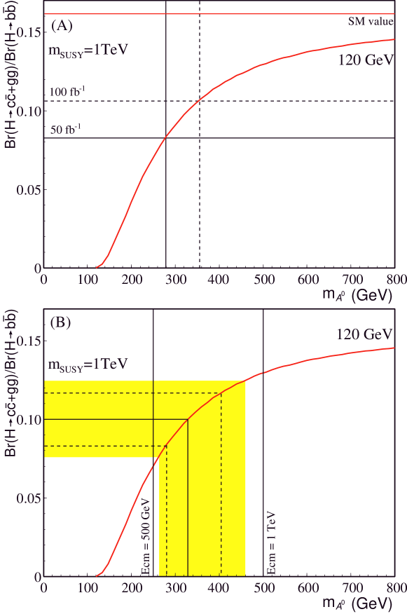
Figure 7: Relation between $Br(H\to c\bar{c},gg)/Br(H\to b\bar{b})$ and $m_{A^{0}}$ for the Higgs boson with a mass of 120 GeV. (A) The solid (dotted) lines show 95 % confidence level lower limit after 1 year (2 years). (B) The shaded area is the allowed region after a year (1 standard deviation). The region in the dotted lines shows the allowed region after two years. Kinematical thresholds for $A^{0}$ direct production are also drawn.

The fact that $Br(H\to\tau^{+}\tau^{-})$ can be measured with a statistical error of 13.4 % corresponds to that $m_{b}$ is determined with an error of 6.7 %. The systematic error of $Br(H\to c\bar{c},gg)/Br(H\to b\bar{b})$ from the uncertainty of $m_{b}$ is estimated to be $\sim$ 10 % after two years. Fig 6 shows the relation between $Br(H\to c\bar{c},gg)/Br(H\to b\bar{b})$ and $m_{b}$.

The relation between $Br(H\to c\bar{c},gg)/Br(H\to b\bar{b})$ and $m_{b}$. The dotted lines show the uncertainty after two years.

7 Summary

We performed a detailed simulation study for the measurement of the ratio $Br(H\to c\bar{c},gg)/Br(H\to b\bar{b})$ at $\sqrt{s}=300$ GeV assuming the JLC standard detector. Here we introduce new approaches to use all decay modes of $Z^{0}$ and to consider the beam polarization. We find that the results obtained from the 2 jet analysis are comparable to those of the 4 jet analysis, although the original event ratio is 2 jet : 4 jet $\sim$ 20 : 70. Thus we can reduce the statistical error by combining the results of all decay modes. On the other hand, the effect of the beam polarization is found to be small for this analysis.

The statistical error of the ratio $Br(H\to c\bar{c},gg)/Br(H\to b\bar{b})$ after two years is estimated to be 17 % for the SM Higgs with a mass of 120 GeV. With the good accuracy of the measurement, we have a chance to rule out the SM, or to constrain the mass of $A^{0}$ in the MSSM, according to the measured value of the ratio.

References

- [1] JLC Group, KEK Report 92-16, December, 1992.
- [2] C. Adolphsen, to be published in Proceedings of the Workshop on Physics and Experiments with Linear Colliders, Morioka-Appi, Japan, September 8-12, 1995.
- [3] M. Leenen, to be published in Proceedings of the Workshop on Physics and Experiments with Linear Colliders, Morioka-Appi, Japan, September 8-12, 1995.
- [4] J.P. Delahaye, to be published in Proceedings of the Workshop on Physics and Experiments with Linear Colliders, Morioka-Appi, Japan, September 8-12, 1995.
- [5] V. Valakin, to be published in Proceedings of the Workshop on Physics and Experiments with Linear Colliders, Morioka-Appi, Japan, September 8-12, 1995.
-
[6]
Y. Okada, M. Yamaguchi and T. Yanagida,
Prog. Theor. Phys. 85 (1991) 1,
Phys. Lett. B262 (1991) 54. - [7] J. Ellis, G. Ridolfi and F. Zwirner, Phys. Lett. B257 (1991) 83.
- [8] H.E. Haber and R. Hempfling, Phys. Rev. Lett. 66 (1991) 1815.
- [9] J. Kamoshita, Y. Okada and M. Tanaka, Phys. Lett. B328 (1994) 67.
- [10] J. Kamoshita, Y. Okada and M. Tanaka, KEK-TH-458, KEK Preprint 95-173.
- [11] M.D. Hildreth et al. , Phys. Rev. D49 3441 (1994).
- [12] Torbjörn Sjöstrand, CERN-TH.7112/93 W5053/W5044.
- [13] T. Ishikawa, T. Kaneko, K. Kato, S. Kawabata, Y. Shimizu and H. Tanaka, “GRACE manual” KEK Report 92-19, February 1993.
- [14] JADE collaboration, W. Bartel et al. , Z. Phys. C33 (1986) 23.