The Azimuthal Decorrelation of Jets Widely Separated in Rapidity

Abstract

This study reports the first measurement of the azimuthal decorrelation between jets with pseudorapidity separation up to five units. The data were accumulated using the DØ detector during the 1992–1993 collider run of the Fermilab Tevatron at $\sqrt{s}=$ 1.8 TeV. These results are compared to next–to–leading order (NLO) QCD predictions and to two leading–log approximations (LLA) where the leading–log terms are resummed to all orders in $\alpha_{\scriptscriptstyle S}$. The final state jets as predicted by NLO QCD show less azimuthal decorrelation than the data. The parton showering LLA Monte Carlo HERWIG describes the data well; an analytical LLA prediction based on BFKL resummation shows more decorrelation than the data.

Correlations between kinematic variables in multijet events provide a simple way to study the complex topologies that occur when more than two jets are present in the final state [3, 4, 5]. For example, in dijet events the two jets exhibit a high degree of correlation, being balanced in transverse energy ($E_{T}$) and back–to–back in azimuth ($\phi$). Deviations from this configuration signal the presence of additional radiation. Theoretically this radiation is described by higher order corrections to the leading order graphs. Using the four momentum transfer $Q^{2}$ in the hard scattering as the characteristic scale and DGLAP [6] evolution in $Q^{2}$, these corrections have been calculated analytically to NLO in perturbative QCD [7, 8]. In addition, they are approximated to all orders by using a parton shower approach, like HERWIG [9] for example. However, there can be more than one characteristic scale in the process. Similar to deep inelastic lepton–hadron scattering at small Bjorken $x$ and large $Q^{2}$, hadron–hadron scattering at large partonic center of mass energies ($\hat{s}$) may require a different theoretical treatment. Instead of just resumming the standard terms involving $\ln Q^{2}$, large terms of the type $\ln(\hat{s}/Q^{2})$ have to be resummed as well using the BFKL technique [10]. Del Duca and Schmidt have done this and predict a different pattern of radiation, which results in an additional decorrelation in the azimuthal angle between two jets, as their distance in pseudorapidity ($\Delta\eta\sim\ln(\hat{s}/Q^{2})$) is increased [4].

In this study, the jets of interest are those most widely separated in pseudorapidity ($\eta=-\ln[\tan(\theta/2)]$, where $\theta$ is the polar angle with respect to the proton beam). The DØ detector [11] is particularly suited for this measurement owing to its uniform calorimetric coverage to $|\eta|\mathrel{\hbox to0.0pt{\raise 1.72218pt\hbox{$<$}\hss}{\lower 3.09999pt\hbox{$\sim$}}}4.0$. The uranium–liquid argon sampling calorimeter facilitates jet identification with its fine transverse segmentation ($0.1\times 0.1$ in $\Delta\eta\times\Delta\phi$). Single particle energy resolutions are $15\%/\sqrt{E}$ and $50\%/\sqrt{E}$ ($E$ in GeV) for electrons and pions, respectively, providing good jet energy resolution.

The data for this study, representing an integrated luminosity of 83 nb^-1, were collected during the 1992–1993 $\overline{p}p$ collider run at the Tevatron with a center of mass energy of $\sqrt{s}=$ 1.8 TeV. The hardware trigger required a single pseudo-projective calorimeter tower ($0.2\times 0.2$ in $\Delta\eta\times\Delta\phi$) to have more than 7 GeV of transverse energy. This trigger was instrumented for $|\eta|<3.2$. Events satisfying this condition were analyzed by an on-line processor farm where a fast version of the jet finding algorithm searched for jets with $E_{T}>30$ GeV.

Jet reconstruction was performed using an iterative fixed cone algorithm. First, the list of calorimeter towers with $E_{T}>1$ GeV (seed towers) was sorted in descending order. Starting with the highest $E_{T}$ seed tower, a precluster was formed from all calorimeter towers with ${\cal R}<0.3$, where ${\cal R}=\sqrt{\Delta\eta^{2}+\Delta\phi^{2}}$ was the distance between tower centers. If a seed tower was included in a precluster, it was removed from the list. This joining was repeated until all seed towers become elements of a precluster. After calculating the $E_{T}$ weighted center of the precluster, the radius of inclusion was increased to 0.7 about this center with all towers in this cone becoming part of the jet. A new jet center was calculated using the $E_{T}$ weighted tower centers. This process was repeated until the jet axis moved less than 0.001 in $\eta$–$\phi$ space between iterations. The final jet $E_{T}$ was defined as the scalar sum of the $E_{T}$ of the towers; its direction was defined using the DØ jet algorithm [12], which differs from the Snowmass algorithm [13]. If any two jets shared more than half of the $E_{T}$ of the smaller $E_{T}$ jet, the jets were merged and the jet center recalculated. Otherwise, any ambiguities in the overlap region were resolved by assigning the energy of a given cell in the shared region to the nearest jet. Jet reconstruction was over 95% efficient for jets with $E_{T}>20$ GeV. Jet energy resolution was 10% at 50 GeV and jet position resolution was less than 0.03 in both $\eta$ and $\phi$.

Accelerator and instrumental backgrounds were removed by cuts on the jet shape. The efficiency for these cuts was greater than 95%. Based on Monte Carlo simulations, residual contamination from backgrounds was estimated to be less than 2%. The jet transverse energy was corrected for energy scale, out–of–cone showering, and underlying event. This correction was based on minimizing the missing transverse energy in direct photon events [14]. Small pseudorapidity biases ($\delta\eta\leq 0.03$), caused by the jet algorithm, were also corrected [15].

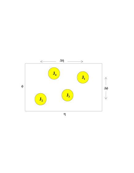
FIG. 1.: Typical event topology in multijet events.

A representative multijet event configuration is shown in Fig. 1. From the sample of jets with $E_{T}>20$ GeV and $|\eta|\leq 3.0$, the two jets at the extremes of pseudorapidity were selected ($J_{1}$ and $J_{2}$ in Fig. 1) for this analysis. One of these two jets was required to be above 50 GeV in $E_{T}$ to remove any trigger inefficiency. The pseudorapidity difference ($\Delta\eta=|\eta_{1}-\eta_{2}|$) distribution for events that pass the cuts is shown in Fig. 2. In Fig.  3, the azimuthal angular separation, $1-\Delta\phi/\pi$ ($\Delta\phi=\phi_{1}-\phi_{2}$) is plotted for unit bins of $\Delta\eta$ centered at $\Delta\eta$ = 1, 3, and 5. Since each distribution is normalized to unity, the decorrelation between the two most widely separated jets can be seen in either the relative decline near the peak or the relative increase in width as $\Delta\eta$ increases.

FIG. 2.: The pseudorapidity interval, $\Delta\eta=|\eta_{1}-\eta_{2}|$, of the two jets at the extremes of pseudorapidity. The coverage extends to $\Delta\eta\sim 6$. The errors are statistical only.

The decorrelation in Fig. 3 can be quantified in terms of the average value of $\cos(\pi-\Delta\phi)$ [3]. Figure 4 shows $\langle\cos(\pi-\Delta\phi)\rangle$ vs. $\Delta\eta$. For the data, the error bars represent the statistical and point–to–point uncorrelated systematic errors added in quadrature. In addition, the band at the bottom of the plot represents the correlated uncertainties of the energy scale and effects due to hadronization and calorimeter resolution. Also shown in Fig. 4 are the predictions from HERWIG, NLO QCD as implemented in JETRAD [8], and the BFKL resummation [4, 16]. The errors shown for the three QCD predictions are statistical only.

The systematic errors, especially the energy scale uncertainty, dominate the statistical errors for all $\Delta\eta$ except for $\Delta\eta=5$. The jet energy scale uncertainty is estimated to be 5%. The resulting uncertainty in $\langle\cos(\pi-\Delta\phi)\rangle$ varied from 0.002 at $\Delta\eta=0$ to 0.011 at $\Delta\eta=5$. Since the out–of–cone corrections depended on the pseudorapidity of the jet and may not be well understood at large pseudorapidities, the full size of the out–of–cone showering correction was included in the energy scale error band. This size of this error was less than 0.013. Uncorrelated systematic uncertainties due to the $\eta$ bias correction and angular resolution were included. This error was less than 0.002. The jet selection cuts introduced a systematic uncertainty less than 0.007, which is independent of $\phi$ and $\eta$. The uncertainty due to jet position reconstruction was estimated by analyzing a subset of the data, specifically events with a large $\Delta\eta$, using both Snowmass and DØ jet finding algorithms; the differences in $\langle\cos(\pi-\Delta\phi)\rangle$ was less than 0.002.

Comparison of theory with data requires the connection of partons with jets. Since no attempt has been made to correct the data back to the parton level, the the size of the hadronization and calorimeter resolution effects were included as an additional systematic error. These effects were estimated using HERWIG with a detector simulation based on GEANT [17]. Jets before hadronization were compared with jets after both hadronization and detector simulation. In both cases a cone jet algorithm with a radius of 0.7 was used. Jets reconstructed using partons and particles produced indistinguishable results for $\langle\cos(\pi-\Delta\phi)\rangle$; the calorimeter smearing effects, although negligible for $\Delta\eta\leq 3$, were $\sim 0.02$ at $\Delta\eta=4$ and $\sim 0.03$ at $\Delta\eta=5$. The size of these effects were included in the correlated systematic error band.

FIG. 3.: The azimuthal angle difference, $\Delta\phi=\phi_{1}-\phi_{2}$, distribution of the two jets at the extremes of pseudorapidity plotted as $1-\Delta\phi/\pi$ for $\Delta\eta=1$, 3, and 5 ($0.5<\Delta\eta<1.5$, $2.5<\Delta\eta<3.5$, and $4.5<\Delta\eta<5.5$). The errors are statistical only.

Since NLO is the first order in perturbative QCD where decorrelation is predicted, it may be sensitive to the choice of cutoff parameters (scales) necessary in a perturbative calculation. Similar effects have been seen in NLO predictions of jet shape [18] and topologies with jets beyond the two body kinematic limit [19]. To estimate the size of these effects, the renormalization and factorization scales in JETRAD were varied simultaneously from $p_{T}^{max}/2$ to $2p_{T}^{max}$, where $p_{T}^{max}$ is the transverse momentum of the leading parton. The predictions for $\langle\cos(\pi-\Delta\phi)\rangle$ varied by less than 0.026. The effect of using different parton distribution functions (CTEQ2M [20], MRSD$-$ [21], and GRV [22]) produced variations in JETRAD that were less than 0.0025. Since NLO QCD might be sensitive to the jet definition, the jet algorithm angle definition study, previously done with data, was repeated using JETRAD. The difference between the Snowmass and DØ definitions was smaller than 0.013 for all $\Delta\eta$.

The data in Fig. 4 show a nearly linear decrease in $\langle\cos(\pi-\Delta\phi)\rangle$ with pseudorapidity interval. For small pseudorapidity intervals both JETRAD and HERWIG describe the data reasonably well. JETRAD, which is leading order in any decorrelation effects, predicts too little decorrelation at large pseudorapidity intervals. The prediction of BFKL leading–log approximation, which is valid for large $\alpha_{\scriptscriptstyle S}\Delta\eta$, is shown for $\Delta\eta\geq 2$. As the pseudorapidity interval increases, this calculation predicts too much decorrelation. Also shown in Fig. 4 is the HERWIG prediction, where higher order effects are modeled with a parton shower. These predictions agree with the data over the entire pseudorapidity interval range ($0\leq\Delta\eta\leq 5$).

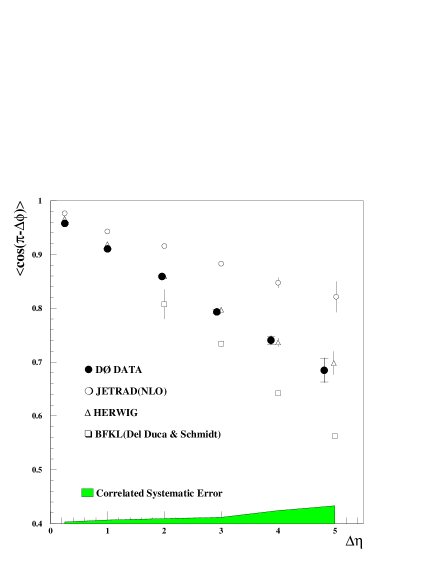
FIG. 4.: The correlation variable used in this analysis, the average value of $\cos(\pi-\Delta\phi)$ vs. $\Delta\eta$, for the data, JETRAD, HERWIG, and the BFKL calculations of Del Duca and Schmidt.

In summary, we have made the first measurement of azimuthal decorrelation as a function of pseudorapidity separation in dijet systems. These results have been compared with various QCD predictions. While the JETRAD predictions showed too little and the BFKL resummation predictions showed too much decorrelation, HERWIG describes the data well over the entire $\Delta\eta$ range studied.

We appreciate the many fruitful discussions with Vittorio Del Duca and Carl Schmidt. We thank the Fermilab Accelerator, Computing, and Research Divisions, and the support staffs at the collaborating institutions for their contributions to the success of this work. We also acknowledge the support of the U.S. Department of Energy, the U.S. National Science Foundation, the Commissariat à L’Energie Atomique in France, the Ministry for Atomic Energy and the Ministry of Science and Technology Policy in Russia, CNPq in Brazil, the Departments of Atomic Energy and Science and Education in India, Colciencias in Colombia, CONACyT in Mexico, the Ministry of Education, Research Foundation and KOSEF in Korea, CONICET and UBACYT in Argentina, and the A.P. Sloan Foundation.

REFERENCES

- [1] Visitor from IHEP, Beijing, China.
- [2] Visitor from Univ. San Francisco de Quito, Ecuador.
- [3] W.J. Stirling, Nucl. Phys. B423, 56 (1994).
- [4] V. Del Duca, C.R. Schmidt, Phys. Rev. D 51, 2150 (1995); Phys. Rev. D 49, 4510 (1994).
- [5] A.H. Mueller, in the Proceedings of the 2nd Workshop on Small-x and Diffractive Physics at the Tevatron (Fermilab, Batavia, IL, USA, Sep. 22-24, 1994).
-
[6]
V.N. Gribov and L.N. Lipatov, Sov. J. Nucl. Phys. 46,
438 (1972);
L.N. Lipatov, Sov. J. Nucl. Phys. 20, 95 (1975);
G. Altarelli and G. Parisi, Nucl. Phys. B126, 298 (1977);
Yu.L. Dokshitzer, Sov. Phys. JETP 46, 641 (1977). - [7] S.D. Ellis, Z. Kunszt, and D.E. Soper, Phys. Rev. Lett. 69, 1496 (1992); Phys. Rev. Lett. 64, 2121 (1990).
- [8] W.T. Giele, E.W.N. Glover, D.A. Kosower, Phys. Rev. Lett. 73, 2019 (1994); Nucl. Phys. B403, 633 (1993).
-
[9]
G. Marchesini, B.R. Webber, Nucl. Phys. B310, 461
(1988);
I.G. Knowles, Nucl. Phys. B310, 571 (1988);
G. Marchesini et al., Comp. Phys. Comm. 67, 465 (1992). -
[10]
L.N. Lipatov, Sov. J. Nucl. Phys. 23, 338 (1976);
E.A. Kuraev, L.N. Lipatov, V.S. Fadin, Sov. Phys. JETP 44, 443 (1976); Sov. Phys. JETP 45, 199 (1977);
Ya.Ya. Balitsky, L.N. Lipatov, Sov. J. Nucl. Phys. 28, 822 (1978). - [11] DØ Collaboration, S. Abachi et al., Nucl. Instrum. Methods A 338, 185 (1994).
- [12] The DØ jet algorithm defines the jet as where the sum is over calorimeter towers in the jet cone. The angles are defined as and where
- [13] J.E. Huth et al., in the Proceedings of the Summer Study on High Energy Physics, Research Direction for the Decade: Snowmass ’90, edited by E.L. Berger (World Sci., Singapore, 1992).
- [14] H. Weerts, in the Proceedings of the 9th Topical Workshop on Proton-Antiproton Collider Physics, edited by K. Kondo and S. Kim (Universal Academy Press, Tokyo, Japan, 1994).
- [15] V.D. Elvira, Ph.D. Thesis (unpublished), Univ. of Buenos Aires, Argentina, 1994.
- [16] V. Del Duca and C.R. Schmidt, private communication.
- [17] R.Brun et al., “GEANT3.14” (unpublished), CERN, DD/EE/84-1.
- [18] DØ collaboration, S. Abachi et al., Phys. Lett. B 357, 500 (1995).
- [19] W.T. Giele, E.W.N Glover, D.A. Kosower, Phys. Rev. D 52, 1486 (1995).
- [20] W.K. Tung, in the Proceedings of the International Workshop on Deep Inelastic Scattering and Related Subjects, Eilat, Israel (World Sci., Singapore, 1994).
- [21] A.D. Martin, W.J. Stirling, R.G. Roberts, Phys. Rev. D 47, 867 (1993).
- [22] A. Vogt, Phys. Lett. B 354, 145 (1995).