Measurement of the Diffractive Cross Section in Deep Inelastic Scattering

Abstract

Diffractive scattering of $\gamma^{*}p\to X+N$, where $N$ is either a proton or a nucleonic system with $M_{N}~{}<~{}4$ GeV has been measured in deep inelastic scattering (DIS) at HERA. The cross section was determined by a novel method as a function of the $\gamma^{*}p$ c.m. energy $W$ between 60 and 245 GeV and of the mass $M_{X}$ of the system $X$ up to 15 GeV at average $Q^{2}$ values of 14 and 31 GeV². The diffractive cross section $d\sigma^{diff}/dM_{X}$ is, within errors, found to rise linearly with $W$. Parameterizing the $W$ dependence by the form $d\sigma^{diff}/dM_{X}\propto(W^{2})^{(2\overline{\mbox{$\alpha_{{}_{IP}}$}}-2)}$ the DIS data yield for the pomeron trajectory $\overline{\mbox{$\alpha_{{}_{IP}}$}}=1.23\pm 0.02(stat)\pm 0.04(syst)$ averaged over $t$ in the measured kinematic range assuming the longitudinal photon contribution to be zero. This value for the pomeron trajectory is substantially larger than $\overline{\mbox{$\alpha_{{}_{IP}}$}}$ extracted from soft interactions. The value of $\overline{\mbox{$\alpha_{{}_{IP}}$}}$ measured in this analysis suggests that a substantial part of the diffractive DIS cross section originates from processes which can be described by perturbative QCD. From the measured diffractive cross sections the diffractive structure function of the proton $F^{D(3)}_{2}(\beta,Q^{2},\mbox{$x_{{}_{IP}}$})$ has been determined, where $\beta$ is the momentum fraction of the struck quark in the pomeron. The form $F^{D(3)}_{2}=constant\cdot(1/\mbox{$x_{{}_{IP}}$})^{a}$ gives a good fit to the data in all $\beta$ and $Q^{2}$ intervals with $a=1.46\pm 0.04(stat)\pm 0.08(syst)$.

DESY 96-018
February 1996

M. Derrick, D. Krakauer, S. Magill, D. Mikunas, B. Musgrave, J.R. Okrasinski, J. Repond, R. Stanek, R.L. Talaga, H. Zhang
Argonne National Laboratory, Argonne, IL, USA ^p
M.C.K. Mattingly
Andrews University, Berrien Springs, MI, USA
G. Bari, M. Basile, L. Bellagamba, D. Boscherini, A. Bruni, G. Bruni, P. Bruni, G. Cara Romeo, G. Castellini¹, L. Cifarelli², F. Cindolo, A. Contin, M. Corradi, I. Gialas, P. Giusti, G. Iacobucci, G. Laurenti, G. Levi, A. Margotti, T. Massam, R. Nania, F. Palmonari, A. Polini, G. Sartorelli,
Y. Zamora Garcia³, A. Zichichi
University and INFN Bologna, Bologna, Italy ^f
C. Amelung, A. Bornheim, J. Crittenden, T. Doeker⁴, M. Eckert, L. Feld, A. Frey, M. Geerts, M. Grothe, H. Hartmann, K. Heinloth, L. Heinz, E. Hilger, H.-P. Jakob, U.F. Katz, S. Mengel, J. Mollen⁵, E. Paul, M. Pfeiffer, Ch. Rembser, D. Schramm, J. Stamm, R. Wedemeyer
Physikalisches Institut der Universität Bonn, Bonn, Germany ^c
S. Campbell-Robson, A. Cassidy, W.N. Cottingham, N. Dyce, B. Foster, S. George, M.E. Hayes, G.P. Heath, H.F. Heath, D. Piccioni, D.G. Roff, R.J. Tapper, R. Yoshida
H.H. Wills Physics Laboratory, University of Bristol, Bristol, U.K. ^o
M. Arneodo⁶, R. Ayad, M. Capua, A. Garfagnini, L. Iannotti, M. Schioppa, G. Susinno
Calabria University, Physics Dept.and INFN, Cosenza, Italy ^f
A. Caldwell⁷, N. Cartiglia, Z. Jing, W. Liu, J.A. Parsons, S. Ritz⁸, F. Sciulli, P.B. Straub, L. Wai⁹, S. Yang¹⁰, Q. Zhu
Columbia University, Nevis Labs., Irvington on Hudson, N.Y., USA  ^q
P. Borzemski, J. Chwastowski, A. Eskreys, M. Zachara, L. Zawiejski
Inst. of Nuclear Physics, Cracow, Poland ^j
L. Adamczyk, B. Bednarek, K. Jeleń, D. Kisielewska, T. Kowalski, M. Przybycień, E. Rulikowska-Zarȩbska, L. Suszycki, J. Zaja̧c
Faculty of Physics and Nuclear Techniques, Academy of Mining and Metallurgy, Cracow, Poland ^j
A. Kotański
Jagellonian Univ., Dept. of Physics, Cracow, Poland ^k
L.A.T. Bauerdick, U. Behrens, H. Beier, J.K. Bienlein, O. Deppe, K. Desler, G. Drews, M. Flasiński¹¹, D.J. Gilkinson, C. Glasman, P. Göttlicher, J. Große-Knetter, T. Haas, W. Hain, D. Hasell, H. Heßling, Y. Iga, K.F. Johnson¹², P. Joos, M. Kasemann, R. Klanner, W. Koch, U. Kötz, H. Kowalski, J. Labs, A. Ladage, B. Löhr, M. Löwe, D. Lüke, J. Mainusch¹³, O. Mańczak, T. Monteiro¹⁴, J.S.T. Ng, D. Notz, K. Ohrenberg, K. Piotrzkowski, M. Roco, M. Rohde, J. Roldán, U. Schneekloth, W. Schulz, F. Selonke, B. Surrow, T. Voß, D. Westphal, G. Wolf, C. Youngman, W. Zeuner
Deutsches Elektronen-Synchrotron DESY, Hamburg, Germany
H.J. Grabosch, A. Kharchilava¹⁵, S.M. Mari¹⁶, A. Meyer, S. Schlenstedt, N. Wulff
DESY-IfH Zeuthen, Zeuthen, Germany
G. Barbagli, E. Gallo, P. Pelfer
University and INFN, Florence, Italy ^f
G. Maccarrone, S. De Pasquale, L. Votano
INFN, Laboratori Nazionali di Frascati, Frascati, Italy ^f
A. Bamberger, S. Eisenhardt, T. Trefzger, S. Wölfle
Fakultät für Physik der Universität Freiburg i.Br., Freiburg i.Br., Germany ^c
J.T. Bromley, N.H. Brook, P.J. Bussey, A.T. Doyle, D.H. Saxon, L.E. Sinclair, M.L. Utley,
A.S. Wilson
Dept. of Physics and Astronomy, University of Glasgow, Glasgow, U.K. ^o
A. Dannemann, U. Holm, D. Horstmann, R. Sinkus, K. Wick
Hamburg University, I. Institute of Exp. Physics, Hamburg, Germany ^c
B.D. Burow¹⁷, L. Hagge¹³, E. Lohrmann, J. Milewski, N. Pavel, G. Poelz, W. Schott, F. Zetsche
Hamburg University, II. Institute of Exp. Physics, Hamburg, Germany ^c
T.C. Bacon, N. Brümmer, I. Butterworth, V.L. Harris, G. Howell, B.H.Y. Hung, L. Lamberti¹⁸, K.R. Long, D.B. Miller, A. Prinias¹⁹, J.K. Sedgbeer, D. Sideris, A.F. Whitfield
Imperial College London, High Energy Nuclear Physics Group, London, U.K. ^o
U. Mallik, M.Z. Wang, S.M. Wang, J.T. Wu
University of Iowa, Physics and Astronomy Dept., Iowa City, USA ^p
P. Cloth, D. Filges
Forschungszentrum Jülich, Institut für Kernphysik, Jülich, Germany
S.H. An, G.H. Cho, B.J. Ko, S.B. Lee, S.W. Nam, H.S. Park, S.K. Park
Korea University, Seoul, Korea ^h
S. Kartik, H.-J. Kim, R.R. McNeil, W. Metcalf, V.K. Nadendla
Louisiana State University, Dept. of Physics and Astronomy, Baton Rouge, LA, USA ^p
F. Barreiro, G. Cases, J.P. Fernandez, R. Graciani, J.M. Hernández, L. Hervás, L. Labarga,
M. Martinez, J. del Peso, J. Puga, J. Terron, J.F. de Trocóniz
Univer. Autónoma Madrid, Depto de Física Teóríca, Madrid, Spain ⁿ
F. Corriveau, D.S. Hanna, J. Hartmann, L.W. Hung, J.N. Lim, C.G. Matthews²⁰, P.M. Patel,
M. Riveline, D.G. Stairs, M. St-Laurent, R. Ullmann, G. Zacek
McGill University, Dept. of Physics, Montréal, Québec, Canada ^{a,  b}
T. Tsurugai
Meiji Gakuin University, Faculty of General Education, Yokohama, Japan
V. Bashkirov, B.A. Dolgoshein, A. Stifutkin
Moscow Engineering Physics Institute, Moscow, Russia  ^l
G.L. Bashindzhagyan²¹, P.F. Ermolov, L.K. Gladilin, Yu.A. Golubkov, V.D. Kobrin, I.A. Korzhavina,
V.A. Kuzmin, O.Yu. Lukina, A.S. Proskuryakov, A.A. Savin, L.M. Shcheglova, A.N. Solomin,
N.P. Zotov
Moscow State University, Institute of Nuclear Physics, Moscow, Russia ^m
M. Botje, F. Chlebana, J. Engelen, M. de Kamps, P. Kooijman, A. Kruse, A. van Sighem, H. Tiecke, W. Verkerke, J. Vossebeld, M. Vreeswijk, L. Wiggers, E. de Wolf, R. van Woudenberg²²
NIKHEF and University of Amsterdam, Netherlands ⁱ
D. Acosta, B. Bylsma, L.S. Durkin, J. Gilmore, C. Li, T.Y. Ling, P. Nylander, I.H. Park, T.A. Romanowski²³
Ohio State University, Physics Department, Columbus, Ohio, USA ^p
D.S. Bailey, R.J. Cashmore²⁴, A.M. Cooper-Sarkar, R.C.E. Devenish, N. Harnew, M. Lancaster, L. Lindemann, J.D. McFall, C. Nath, V.A. Noyes¹⁹, A. Quadt, J.R. Tickner, H. Uijterwaal,
R. Walczak, D.S. Waters, F.F. Wilson, T. Yip
Department of Physics, University of Oxford, Oxford, U.K. ^o
G. Abbiendi, A. Bertolin, R. Brugnera, R. Carlin, F. Dal Corso, M. De Giorgi, U. Dosselli,
S. Limentani, M. Morandin, M. Posocco, L. Stanco, R. Stroili, C. Voci, F. Zuin
Dipartimento di Fisica dell’ Universita and INFN, Padova, Italy ^f
J. Bulmahn, R.G. Feild²⁵, B.Y. Oh, J.J. Whitmore
Pennsylvania State University, Dept. of Physics, University Park, PA, USA ^q
G. D’Agostini, G. Marini, A. Nigro, E. Tassi
Dipartimento di Fisica, Univ. ’La Sapienza’ and INFN, Rome, Italy ${}^{f}~{}$
J.C. Hart, N.A. McCubbin, T.P. Shah
Rutherford Appleton Laboratory, Chilton, Didcot, Oxon, U.K. ^o
E. Barberis, T. Dubbs, C. Heusch, M. Van Hook, W. Lockman, J.T. Rahn, H.F.-W. Sadrozinski, A. Seiden, D.C. Williams
University of California, Santa Cruz, CA, USA ^p
J. Biltzinger, R.J. Seifert, O. Schwarzer, A.H. Walenta, G. Zech
Fachbereich Physik der Universität-Gesamthochschule Siegen, Germany ^c
H. Abramowicz, G. Briskin, S. Dagan²⁶, A. Levy²¹
School of Physics,Tel-Aviv University, Tel Aviv, Israel  ^e
J.I. Fleck²⁷, M. Inuzuka, T. Ishii, M. Kuze, S. Mine, M. Nakao, I. Suzuki, K. Tokushuku, K. Umemori, S. Yamada, Y. Yamazaki
Institute for Nuclear Study, University of Tokyo, Tokyo, Japan ^g
M. Chiba, R. Hamatsu, T. Hirose, K. Homma, S. Kitamura²⁸, T. Matsushita, K. Yamauchi
Tokyo Metropolitan University, Dept. of Physics, Tokyo, Japan ^g
R. Cirio, M. Costa, M.I. Ferrero, S. Maselli, C. Peroni, R. Sacchi, A. Solano, A. Staiano
Universita di Torino, Dipartimento di Fisica Sperimentale and INFN, Torino, Italy ^f
M. Dardo
II Faculty of Sciences, Torino University and INFN - Alessandria, Italy ^f
D.C. Bailey, F. Benard, M. Brkic, G.F. Hartner, K.K. Joo, G.M. Levman, J.F. Martin, R.S. Orr, S. Polenz, C.R. Sampson, D. Simmons, R.J. Teuscher
University of Toronto, Dept. of Physics, Toronto, Ont., Canada ^a
J.M. Butterworth, C.D. Catterall, T.W. Jones, P.B. Kaziewicz, J.B. Lane, R.L. Saunders, J. Shulman, M.R. Sutton
University College London, Physics and Astronomy Dept., London, U.K. ^o
B. Lu, L.W. Mo
Virginia Polytechnic Inst. and State University, Physics Dept., Blacksburg, VA, USA ^q
W. Bogusz, J. Ciborowski, J. Gajewski, G. Grzelak²⁹, M. Kasprzak, M. Krzyżanowski,
K. Muchorowski³⁰, R.J. Nowak, J.M. Pawlak, T. Tymieniecka, A.K. Wróblewski, J.A. Zakrzewski, A.F. Żarnecki
Warsaw University, Institute of Experimental Physics, Warsaw, Poland ^j
M. Adamus
Institute for Nuclear Studies, Warsaw, Poland ^j
C. Coldewey, Y. Eisenberg²⁶, U. Karshon²⁶, D. Revel²⁶, D. Zer-Zion
Weizmann Institute, Particle Physics Dept., Rehovot, Israel ^d
W.F. Badgett, J. Breitweg, D. Chapin, R. Cross, S. Dasu, C. Foudas, R.J. Loveless, S. Mattingly, D.D. Reeder, S. Silverstein, W.H. Smith, A. Vaiciulis, M. Wodarczyk
University of Wisconsin, Dept. of Physics, Madison, WI, USA ^p
S. Bhadra, M.L. Cardy, C.-P. Fagerstroem, W.R. Frisken, M. Khakzad, W.N. Murray, W.B. Schmidke
York University, Dept. of Physics, North York, Ont., Canada ^{a
  1} also at IROE Florence, Italy
  ² now at Univ. of Salerno and INFN Napoli, Italy
  ³ supported by Worldlab, Lausanne, Switzerland
  ⁴ now as MINERVA-Fellow at Tel-Aviv University
  ⁵ now at ELEKLUFT, Bonn
   ⁶ also at University of Torino
  ⁷ Alexander von Humboldt Fellow
  ⁸ Alfred P. Sloan Foundation Fellow
  ⁹ now at University of Washington, Seattle
¹⁰ now at California Institute of Technology, Los Angeles
¹¹ now at Inst. of Computer Science, Jagellonian Univ., Cracow
¹² visitor from Florida State University
¹³ now at DESY Computer Center
¹⁴ supported by European Community Program PRAXIS XXI
¹⁵ now at Univ. de Strasbourg
¹⁶ present address: Dipartimento di Fisica, Univ. ”La Sapienza”, Rome
¹⁷ also supported by NSERC, Canada
¹⁸ supported by an EC fellowship
¹⁹ PPARC Post-doctoral Fellow
²⁰ now at Park Medical Systems Inc., Lachine, Canada
²¹ partially supported by DESY
²² now at Philips Natlab, Eindhoven, NL
²³ now at Department of Energy, Washington
²⁴ also at University of Hamburg, Alexander von Humboldt Research Award
²⁵ now at Yale University, New Haven, CT
²⁶ supported by a MINERVA Fellowship
²⁷ supported by the Japan Society for the Promotion of Science (JSPS)
²⁸ present address: Tokyo Metropolitan College of Allied Medical Sciences, Tokyo 116, Japan
²⁹ supported by the Polish State Committee for Scientific Research, grant No. 2P03B09308
³⁰ supported by the Polish State Committee for Scientific Research, grant No. 2P03B09208

a	supported by the Natural Sciences and Engineering Research Council of Canada (NSERC)
b	supported by the FCAR of Québec, Canada
c	supported by the German Federal Ministry for Education and Science, Research and Technology (BMBF), under contract numbers 056BN19I, 056FR19P, 056HH19I, 056HH29I, 056SI79I
d	supported by the MINERVA Gesellschaft für Forschung GmbH, and by the Israel Academy of Science
e	supported by the German Israeli Foundation, and by the Israel Academy of Science
f	supported by the Italian National Institute for Nuclear Physics (INFN)
g	supported by the Japanese Ministry of Education, Science and Culture (the Monbusho) and its grants for Scientific Research
h	supported by the Korean Ministry of Education and Korea Science and Engineering Foundation
i	supported by the Netherlands Foundation for Research on Matter (FOM)
j	supported by the Polish State Committee for Scientific Research, grants No. 115/E-343/SPUB/P03/109/95, 2P03B 244 08p02, p03, p04 and p05, and the Foundation for Polish-German Collaboration (proj. No. 506/92)
k	supported by the Polish State Committee for Scientific Research (grant No. 2 P03B 083 08)
l	partially supported by the German Federal Ministry for Education and Science, Research and Technology (BMBF)
m	supported by the German Federal Ministry for Education and Science, Research and Technology (BMBF), and the Fund of Fundamental Research of Russian Ministry of Science and Education and by INTAS-Grant No. 93-63
n	supported by the Spanish Ministry of Education and Science through funds provided by CICYT
o	supported by the Particle Physics and Astronomy Research Council
p	supported by the US Department of Energy
q	supported by the US National Science Foundation

1 Introduction

In deep-inelastic electron-proton scattering (DIS), $e^{-}p\rightarrow e^{-}$ + anything (Fig. 1), a new class of events was observed by ZEUS [1, 2, 3] and H1 [4] characterized by a large rapidity gap (LRG) between the direction of the proton beam and the angle of the first significant energy deposition in the detector. The properties of these events indicate a diffractive and leading twist production mechanism. The observation of jet production demonstrated that there is a hard scattering component in virtual-photon proton interactions leading to LRG events. A comparison of the energy flow in events with and without a large rapidity gap showed that in LRG events the QCD radiative processes are suppressed.

The diffractive contribution to the proton structure function $F_{2}$ was measured by H1 [5] and ZEUS [6]. The diffractive electron-proton cross section was found to be consistent with factorising into a term describing the flux of a colourless component in the proton and a term which describes the cross section for scattering of this colourless object on an electron. LRG events were also observed in photoproduction [7, 8]. A combined analysis of the diffractive part of the proton structure function $F_{2}$ and the diffractive photoproduction of jets indicated that a large fraction of the momentum of the colourless object carried by partons is due to hard gluons [9].

One of the most interesting questions raised by these LRG events is the precise $W$ dependence of the cross section for diffractive scattering of virtual photons on protons, $\gamma^{*}p\to Xp$. Here, $W$ is the $\gamma^{*}p$ c.m. energy and the comparison should be done at fixed mass squared of the virtual photon, $-Q^{2}$. In the Regge picture, the elastic and diffractive cross sections in the forward direction are expected to behave as (see e.g. [10]):

$$d\sigma(t=0)/dt\propto(W^{2})^{2\mbox{$\alpha_{{}_{IP}}$}(0)-2}\;\;\;,$$ (1)

where $t$ is the square of the four-momentum transferred from the virtual photon to the incoming proton. From elastic and total cross section measurements for hadron-hadron scattering the intercept $\mbox{$\alpha_{{}_{IP}}$}(0)$ of the pomeron trajectory $\mbox{$\alpha_{{}_{IP}}$}(t)$ was found to be 1.08 [11]. A similar energy dependence was observed for diffractive dissociation in hadron-hadron scattering of the type $h_{1}h_{2}\rightarrow h_{1}X$, for a fixed mass $M_{X}$ of the diffractively produced system $X$ (see e.g. [12, 13]). For DIS, with dominantly hard partonic interactions, the BFKL formalism [14] leads to a pomeron intercept of $\mbox{$\alpha_{{}_{IP}}$}(0)\approx 1+(12\;\ln 2)\alpha_{s}/\pi\approx 1.5$ at $Q^{2}=20$ GeV² which could imply a rapid rise of the diffractive cross section with $W$ [15, 16].

In the previous determinations of the diffractive structure function, the subtraction of the nondiffractive contribution relied on specific models [5, 6]. In the present analysis the separation is based on the data. The diffractive contr

ibution is extracted by a new method which uses the mass $M_{X}$ of the system $X$, measured in the detector, to separate the diffractive and nondiffractive contributions. The distribution in $\ln M^{2}_{X}$ exhibits, for the nondiffractive component, an exponential fall-off towards small $\ln M^{2}_{X}$ values, $dN^{nondiff}/d\ln M^{2}_{X}\propto\exp(b$ $\ln M^{2}_{X})$, a property which is predicted by QCD-based models for nondiffractive DIS (see e.g. [17, 18]). The parameter $b$ of this exponential fall-off is determined from the data and is assumed to be valid in the region of overlap between the diffractive and nondiffractive components, so allowing subtraction of the nondiffractive background.

The cross section for diffractive production by virtual photons on protons, $\gamma^{*}p\to XN$, is determined integrated over $t$. The system $N$ is either a proton or a nucleonic system with mass $M_{N}<4$ GeV. The 4 GeV mass limit results from the acceptance of the detector.

The prime goal of this analysis is the determination of the $W$ dependence of the diffractive $\gamma^{*}p$ cross section in the range $60<W<245$ GeV, $M_{X}<15$ GeV and $10<Q^{2}<56$ GeV². The paper begins with a brief introduction to the experimental setup and the event selection procedure followed by a description of the determination of the mass $M_{X}$. Using the measured $M_{X}$ distributions, the widely different behaviour of the nondiffractive and diffractive contributions is demonstrated: production of events with low masses $M_{X}$ is dominated by diffractive scattering while nondiffractive events are concentrated at large $M_{X}$ values. These observations lead to a straightforward procedure for extrapolating the nondiffractive background into the low mass region and extracting the diffractive contribution. An unfolding procedure is used to correct the resulting number of diffractive events in $(M_{X},W,Q^{2})$ bins for detector acceptance and migration effects. From the corrected number of events the cross sections for diffractive production by virtual-photon proton scattering are obtained and the $W$ dependence of diffractive scattering is determined. Finally, the cross sections are analyzed in terms of the diffractive structure function of the proton.

2 Experimental setup

The experiment was performed at the electron-proton collider HERA using the ZEUS detector. The analysis used data taken in 1993 where electrons of $E_{e}=26.7$ GeV collided with protons of $E_{p}=820$ GeV. HERA is designed to run with 210 bunches in each of the electron and proton rings. In 1993, 84 paired bunches were filled for each beam and in addition 10 electron and 6 proton bunches were left unpaired for background studies. The integrated luminosity was 543 nb^-1. Details on the operation of HERA and the detector can be found in [19].

2.1 ZEUS detector

The analysis relies mainly on the high-resolution depleted-uranium scintillator calorimeter and the central tracking detectors. The calorimeter covers 99.7% of the solid angle. It is divided into three parts, forward (FCAL) covering the pseudorapidity region $4.3\geq\eta\geq 1.1$, barrel (BCAL) covering the central region $1.1\geq\eta\geq-0.75$ and rear (RCAL) covering the backward region $-0.75\geq\eta\geq-3.8$. Holes of $20\times 20$ cm² in the center of FCAL and RCAL are required to accommodate the HERA beam pipe. The calorimeter parts are subdivided into towers of typically $20\times 20$ cm² transverse dimensions, which in turn are segmented in depth into electromagnetic (EMC) and hadronic (HAC) sections. To improve spatial resolution, the electromagnetic sections are subdivided transversely into cells of typically $5\times 20$ cm² ($10\times 20$ cm² for the rear calorimeter). Each cell is read out by two photomultiplier tubes, providing redundancy and a position measurement within the cell. Under test beam conditions [20], the calorimeter has an energy resolution, $\sigma_{E}$, given by $\sigma_{E}/E=18\%/\sqrt{E}$ for electrons and $\sigma_{E}/E=35\%/\sqrt{E}$ for hadrons, where $E$ is in units of GeV. In addition, the calorimeter cells provide time measurements with a time resolution below 1 ns for energy deposits greater than 4.5 GeV, a property used in background rejection. The calorimeter noise, dominated by the uranium radioactivity, in average is in the range 15-19 MeV for electromagnetic cells and 24-30 MeV for hadronic cells. The calorimeter is described in detail in [20].

Charged particle detection is performed by two concentric cylindrical drift chambers, the vertex detector (VXD) and the central tracking detector (CTD) occupying the space between the beam pipe and the superconducting coil of the magnet. The detector was operated with a magnetic field of 1.43 T. The CTD consists of 72 cylindrical drift chamber layers organized into 9 superlayers [21]. In events with charged particle tracks, using the combined data from both chambers, resolutions of $0.4$ cm in $Z$ and $0.1$ cm in radial direction in the $XY$ plane are obtained for the primary vertex reconstruction. From Gaussian fits to the $Z$ vertex distribution, the rms spread is found to be $10.5$ cm in agreement with the expectation from the proton bunch length.

The luminosity is determined by measuring the rate of energetic bremsstrahlung photons produced in the process $ep\to ep\gamma$ [22]. The photons are detected in a lead-scintillator calorimeter placed at $Z=-107$ m. The background rate from collisions with the residual gas in the beam pipe was subtracted using the unpaired electron and proton bunches.

2.2 Kinematics

The basic quantities used for the description of inclusive deep inelastic scattering

$$e(k)+p(P)\to e(k^{\prime})+anything$$

are:

$${Q^{2}} = -q^{2}=-(k-k^{\prime})^{2}\;\;\;,$$ (2)

$$x = \frac{\mbox{${Q^{2}}$}}{2P\cdot q}\;\;\;,$$ (3)

$$y = \frac{P\cdot q}{P\cdot k}\;\;\;,$$ (4)

$$W^{2} = \frac{Q^{2}(1-x)}{x}+M_{p}^{2}\approx\frac{\mbox{${Q^{2}}$}}{x}\;{\rm for}\;x\ll 1\;\;\;,$$ (5)

where $k$ and $k^{\prime}$ are the four-momenta of the initial and final state electrons, $P$ is the initial state proton four-momentum, $M_{p}$ is the proton mass, $y$ is the fractional energy transfer to the proton in its rest frame and $W$ is the $\gamma^{*}p$ c.m. energy. For the range of $Q^{2}$ and $W$ considered in this paper we also have $W^{2}\approx y\cdot s$, where $s=4E_{e}E_{p}$ is the square of the $ep$ c.m. energy, $\sqrt{s}=296$ GeV.

For the description of the diffractive processes,

$$ep\to e+X+N,$$

in addition to the mass $M_{X}$, two further variables are introduced:

$$x_{{}_{IP}} = \frac{M^{2}_{X}+Q^{2}}{W^{2}+Q^{2}}\;\;\;,$$ (6)

$$\beta = \frac{Q^{2}}{M^{2}_{X}+Q^{2}}\;\;\;.$$ (7)

In models where diffraction is described by the exchange of a particle-like pomeron, $x_{{}_{IP}}$ is the momentum fraction of the pomeron in the proton and $\beta$ is the momentum fraction of the struck quark within the pomeron.

The kinematic variables $x$, $Q^{2}$ and $W$ were determined with the double angle (DA) method [23], in which only the angles of the scattered electron ($\theta^{\prime}_{e}$) and the hadronic system ($\gamma_{H}$) are used. This reduces the sensitivity to energy scale uncertainties. The angle $\gamma_{H}$ characterizes the transverse and longitudinal momenta of the hadronic system. In the naïve quark-parton model $\gamma_{H}$ is the scattering angle of the struck quark. It was determined from the hadronic energy flow measured in the calorimeter. A momentum vector $\vec{p}_{h}\equiv(p_{{\rm X}},p_{{\rm Y}},p_{{\rm Z}})$ was assigned to each cell $h$ with energy $E$ in such a way that $\vec{p}_{h}^{2}=E^{2}$. The cell angles were calculated from the geometric center of the cell and the vertex position of the event. The angle $\gamma_{H}$ was calculated according to

$$\cos\gamma_{H}=\frac{(\sum_{h}p_{{\rm X}})^{2}+(\sum_{h}p_{{\rm Y}})^{2}-(\sum_{h}(E-p_{{\rm Z}}))^{2}}{(\sum_{h}p_{{\rm X}})^{2}+(\sum_{h}p_{{\rm Y}})^{2}+(\sum_{h}(E-p_{{\rm Z}}))^{2}},$$ (8)

where the sums, $\sum_{h}$, here and in the following, run over all calorimeter cells $h$ which were not assigned to the scattered electron. The cells were required to have energy deposits above 60 MeV in the EMC section and 110 MeV in the HAC section and to have energy deposits above 140 MeV (160 MeV) in the EMC (HAC) sections, if these energy deposits were isolated. The last two cuts remove noise caused by the uranium radioactivity which affects the reconstruction of the DA variables at low $M_{X}$.

In the double angle method, in order that the hadronic system be well measured, it is necessary to require a minimum of hadronic activity in the calorimeter away from the forward direction. A suitable quantity for this purpose is the hadronic estimator of the variable $y$ [24], defined by

$$y_{{}_{JB}}=\frac{\sum_{h}\left(E-p_{{\rm Z}}\right)}{2E_{e}}.$$ (9)

We study below events of the type

$$ep\to e+X+rest,$$

where $X$ denotes the hadronic system observed in the detector and $rest$ the particle system escaping detection through the beam holes. The mass $M_{X}$ of the system $X$ is determined from the energy deposited in the CAL cells according to:

$$(M_{X}^{meas})^{2}=(\sum_{h}E)^{2}-(\sum_{h}p_{X})^{2}-(\sum_{h}p_{Y})^{2}-(\sum_{h}p_{Z})^{2}\;\;\;.$$ (10)

2.3 Event selection

The event selection at the trigger level was identical to that used for our $F_{2}$ analysis [19]. The off-line cuts were very similar to those applied in the double angle analysis of $F_{2}$ [19]. The resulting event sample is also almost identical to the one used for our recent studies of large rapidity gap events in DIS [2, 3]. For ease of reference we list the main kinematic requirements imposed, which limit the $W$ and $Q^{2}$ range of the measurement:

• $E^{\prime}_{e}>$ 8 GeV, where $E^{\prime}_{e}$ is the energy of the scattered electron, to have reliable electron finding and to control the photoproduction background;

• $y_{e}<0.95$, where $y_{e}$ is the variable $y$ calculated from the scattered electron, to reject spurious low energy electrons, especially in the forward direction,

• the impact point of the electron on the face of the RCAL had to lie outside a square of side 32 cm centered on the beam axis (“box cut”), to ensure full containment of the electron shower,

• $y_{JB}>0.02$, to ensure a good measurement of the angle $\gamma_{H}$ and of $x$,

• $35<\delta<60$ GeV, where $\delta=\sum_{h}\left(E-p_{Z}\right)$, to control radiative corrections and reduce photoproduction background.

The differences with respect to the event selection used for the $F_{2}$ analysis in  [19] are an increase of the lower limit on $E^{\prime}_{e}$ from 5 to 8 GeV and a lowering of the $y_{JB}$ cut from 0.04 to 0.02 which became possible with the improved noise suppression procedure explained above. The increase of the $E^{\prime}_{e}$ limit reduces background from photoproduction; the lower $y_{JB}$ cut extends the acceptance towards lower $W$ values. It was checked that the $F_{2}$ values obtained with the modified noise procedure were fully compatible with the values published previously [19] in the whole $Q^{2}$, $W$ range investigated in the present paper.

The primary event vertex was determined from tracks reconstructed using VXD+CTD information. If no tracking information was present the vertex position was set to the nominal interaction point.

After the selection cuts and the removal of QED Compton scattering events and residual cosmic-ray events, the DIS sample contained 46k events. For the analysis of diffractive scattering, events with $Q^{2}>10$ GeV² were used. The background from beam gas scattering in this sample was less than 1% as found from the data taken with unpaired bunches.

3 Simulation and method of analysis

3.1 Monte Carlo simulation

Monte Carlo simulations were used for unfolding the produced event distributions from the measured ones, for determining the acceptance and for estimating systematic uncertainties.

Events from standard DIS processes with first order electroweak corrections were generated with HERACLES 4.4 [25]. It was interfaced using Django 6.0 [26] to ARIADNE 4.03 [17] for modelling the QCD cascade according to the version of the colour dipole model that includes the boson-gluon fusion diagram, denoted by CDMBGF. The fragmentation into hadrons was performed with the Lund fragmentation scheme [18] as implemented in JETSET 7.2 [27]. The parton densities of the proton were chosen to be the MRSD^′- set [28]. Note that this Monte Carlo code does not contain contributions from diffractive $\gamma^{*}p$ interactions.

In order to model the DIS hadronic final states from diffractive interactions where the proton does not dissociate,

$$ep\to e+X+p,$$

two Monte Carlo event samples were studied, one of which was generated by POMPYT 1.0 [29]. POMPYT is a Monte Carlo realization of factorizable models for high energy diffractive processes where, within the PYTHIA 5.6 [30] framework, the beam proton emits a pomeron, whose constituents take part in a hard scattering process with the virtual-photon. For the quark momentum density in the pomeron it has been common to use the so-called Hard POMPYT version, $\beta f(\beta)\propto\beta\cdot(1-\beta)$. For this analysis the form

$$\beta f(\beta)=constant\cdot\beta$$ (11)

was used which enhances the rate of low $M_{X}$ events as preferred by the data.

The second sample was generated following the Nikolaev-Zakharov (NZ) model [31] which was interfaced to the Lund fragmentation scheme [32]. In the NZ model, the exchanged virtual photon fluctuates into a $q\bar{q}$ pair or a $q\bar{q}g$ state which interacts with a colourless two-gluon system emitted by the incident proton. In the Monte Carlo implementation of this model the mass spectrum contains both components but the $q\bar{q}g$ states are fragmented into hadrons as if they were a $q\bar{q}$ system with the same mass $M_{X}$. Hadronic final states $X$ are generated only with masses $M_{X}>$ 1.7 GeV. For a description of the NZ model see also [6].

All Monte Carlo events were passed through the standard ZEUS detector and trigger simulations and the event reconstruction package.

3.2 Weighting of diffractive Monte Carlo events

In order to determine from the number of observed events the number of produced events in each bin an unfolding procedure based on a weighted Monte Carlo sample was applied. The unfolding procedure is most reliable if the Monte Carlo event distributions are in agreement with the data. POMPYT was used for unfolding. However, POMPYT as well as the NZ model showed considerable discrepancies relative to the measured $W$ distributions in the kinematic range of this study. This problem was overcome as follows: to account for the lack of diffractive events in the low mass region, $M_{X}<1$ GeV, events were generated separately for $\rho^{o}$ production via $\gamma^{*}p\to\rho^{o}p$ [33] and added to the POMPYT event sample. The number of $\rho^{o}$ events and their distribution as a function of $W$ and $Q^{2}$ were determined from the analysis of this experiment [34]. Furthermore, the POMPYT and $\rho^{o}$ events were weighted to agree with a Triple Regge [35, 36] inspired model (TRM) predicting for the diffractive cross section:

$$\frac{d\sigma^{diff}_{\gamma^{*}p\to XN}(M_{X},W,Q^{2})}{dM_{X}} = C\cdot(1+c_{L}\cdot Q^{2}/M_{X}^{2})\,(M_{0}^{2}+Q^{2})^{-\alpha_{k}(0)}(M_{X}^{2}/(M_{X}^{2}+Q^{2}))$$ (12)

$$\cdot\frac{M_{X}}{(M_{X}^{2}+Q^{2})^{2-\alpha_{k}(0)}}\cdot(\frac{W^{2}}{M_{X}^{2}+Q^{2}})^{2\overline{\mbox{$\alpha_{{}_{IP}}$}}-2}.$$

Here $C$ is a normalization constant, $\alpha_{k}(0)=0$ ($\alpha_{k}(0)=1$) for $M_{X}<M_{0}$ ($M_{X}\geq M_{0}$) and $\overline{\mbox{$\alpha_{{}_{IP}}$}}$ is the pomeron trajectory averaged over the square of the four-momentum transfer, $t$, between the incoming and the outgoing proton. The parameters $c_{L}$, $M_{0}$, $\overline{\mbox{$\alpha_{{}_{IP}}$}}$ of the TRM model were determined in the unfolding (see section 5 below) and will be referred to as “weighting parameters”. The weighted sample of POMPYT events will be referred to as “weighted POMPYT”.

3.3 Mass determination

The mass of the system $X$ was determined from the energy deposits in the calorimeter using Eq. 10. The mass $M_{X}^{meas}$ measured in this way has to be corrected for energy losses in the inactive material in front of the calorimeter and for acceptance. The correction was determined by comparing for Monte Carlo (MC) generated events the MC measured mass, $M_{X}^{MCmeas}$, to the generated mass, $M_{X}^{MCgen}$, of the system $X$. The mass correction was performed in two steps. In the first step an overall mass correction factor was determined. In the second step the diffractive cross sections were determined by an unfolding procedure (see section 5) taking into account for each ($M_{X},W,Q^{2}$) interval the proper mass correction as determined from the MC simulation.

The overall correction factor $f(M_{X})$ was determined from the average ratio of measured to generated mass $M_{X}$,

$$f(M_{X}^{MCmeas})=\frac{M_{X}^{MCmeas}}{M_{X}^{MCgen}}\;\;\;,$$

as a function of $M_{X}$, $W$ and $Q^{2}$. The dependence of $f(M_{X}^{MCmeas})$ on $M_{X},W,Q^{2}$ was found to be sufficiently small ($\pm 6\%$) for $M_{X}>1.5$ GeV so that it could be neglected in the first step of the mass correction. The average correction factor was $f(M_{X}^{MCmeas})=0.68$. The same correction factor was used for masses below 1.5 GeV. The correction factor $f=0.68$ was applied to obtain from the measured mass the corrected mass value, $M_{X}^{cor}=M_{X}^{meas}/f$.

Figures 2a,b show, for MC events, the corrected versus the generated $M_{X}$. The error bars in Fig. 2b give the rms resolution for a single $M_{X}$ measurement. A tight correlation between corrected and generated mass is observed except when $M_{X}<2$ GeV where the mass resolution is comparable to the value of the mass. The mass resolution increases smoothly from $1$ GeV near the $\rho$ mass to $1.3$ GeV ($2.9$ GeV) at $M_{X}=3$ GeV ($15$ GeV). For $M_{X}^{MCgen}>3$ GeV it can be approximated by $\sigma(M_{X}^{MCcor})/\sqrt{M_{X}^{MCgen}}=0.75$ GeV^1/2.

A test of the MC predictions for the mass measurement at low $M_{X}$ values was performed by studying the reaction

$$ep\to e+\rho^{o}+p\;\;\;,$$

where the pions from the decay $\rho^{o}\to\pi^{+}\pi^{-}$ were measured with the central tracking detector [34]. The $\pi^{+}\pi^{-}$ mass resolution from tracking was 25 MeV(rms). From a total of 60 events with $700<M_{\rho^{o}}^{tracking}<800$ MeV in the kinematic range $Q^{2}=7-25$ GeV², $W=60-134$ GeV, an average $M_{X}^{cor}$ of $1.2$ GeV and an average mass resolution $\sigma(M_{X}^{cor})$ of 0.9 GeV were obtained; all but 4 events were reconstructed with a mass $M^{cor}_{X}$ below 3.0 GeV. The Monte Carlo simulation for this channel predicted $M_{X}^{MCcor}=1.2$ GeV and $\sigma(M_{X}^{MCcor})=0.8$ GeV, in good agreement with the data.

All $M_{X}$ results presented below refer to $M_{X}^{cor}$.

3.4 Acceptance for diffractive events

A measure of the acceptance for diffractive events is the ratio ${\cal R}={\cal N}^{MCmeas}/{\cal N}^{MCgen}$ of events measured to events generated in an ($M_{X},W,Q^{2}$) bin using $M^{cor}_{X}$. Figures 3 and 4 show, for weighted POMPYT events, the distributions of ${\cal N}^{MCgen}$ (histograms) and ${\cal N}^{MCmeas}$ (solid points) for the ($W$, $Q^{2}$) bins used in this analysis (see section 4.1). Here, the generated values for $M_{X},W,Q^{2}$ were used for ${\cal N}^{MCgen}$ while $M_{X}^{cor}$ and the double-angle quantities for $W$ and $Q^{2}$ were used for ${\cal N}^{MCmeas}$, as in the analysis of the data. The $M_{X}$ distributions increase from small $M_{X}$ values to a maximum at $M_{X}=2-5$ GeV and then fall off towards higher masses. There is some leakage of events into the low $M_{X}$ bin as seen in the ratio $\cal R$ shown in the right-hand parts of Figs. 3, 4.

The shaded areas mark the $M_{X}$ regions used for extraction of the diffractive cross sections. The ratio $\cal R$ is above unity at small $M_{X}$ as a result of the migration from higher $M_{X}$ masses; for larger $M_{X}$ values $\cal R$ is rather constant and between $70$ and $100\%$ in the bins considered for the analysis, except in the highest $W$ interval for $Q^{2}=14$ GeV² where the acceptance is around $80\%$ at low masses falling to about $50\%$ at $M_{X}=15$ GeV. This is caused by the reduced efficiency for detecting the scattered electron and by the requirement that $\delta=\sum_{h}(E-p_{Z})>35$ GeV.

3.5 General characteristics of the $M_{X}$ distributions

The method of separating the diffractive and nondiffractive contributions is based on their very different $M_{X}$ distributions. As a first illustration, Fig. 5 shows the distribution of $M_{X}$ versus $W$ for the data. Two distinct classes of events are observed, one concentrated at small $M_{X}$, the second extending to large values of $M_{X}$. Most of the events in the low $M_{X}$ region exhibit a large rapidity gap, which is characteristic of diffractive production. This is shown by Fig. 5 where the events with a large (small) rapidity gap, $\eta_{max}<1.5$ ( $\eta_{max}>1.5$) are marked by different symbols. Here $\eta_{max}$ is the pseudorapidity of the most forward going particle. For this analysis a particle is defined as an isolated set of adjacent calorimeter cells with more than 400 MeV summed energy, or a track observed in the central track detector with more than 400 MeV momentum. A cut of $\eta_{max}<1.5$ corresponds to a visible rapidity gap larger than 2.2 units since no particles were observed between the forward edge of the calorimeter ($\eta=3.7-4.3$) and $\eta=1.5$. For $\eta_{max}<1.5$ the contribution from nondiffractive scattering is expected to be negligible [1, 6].

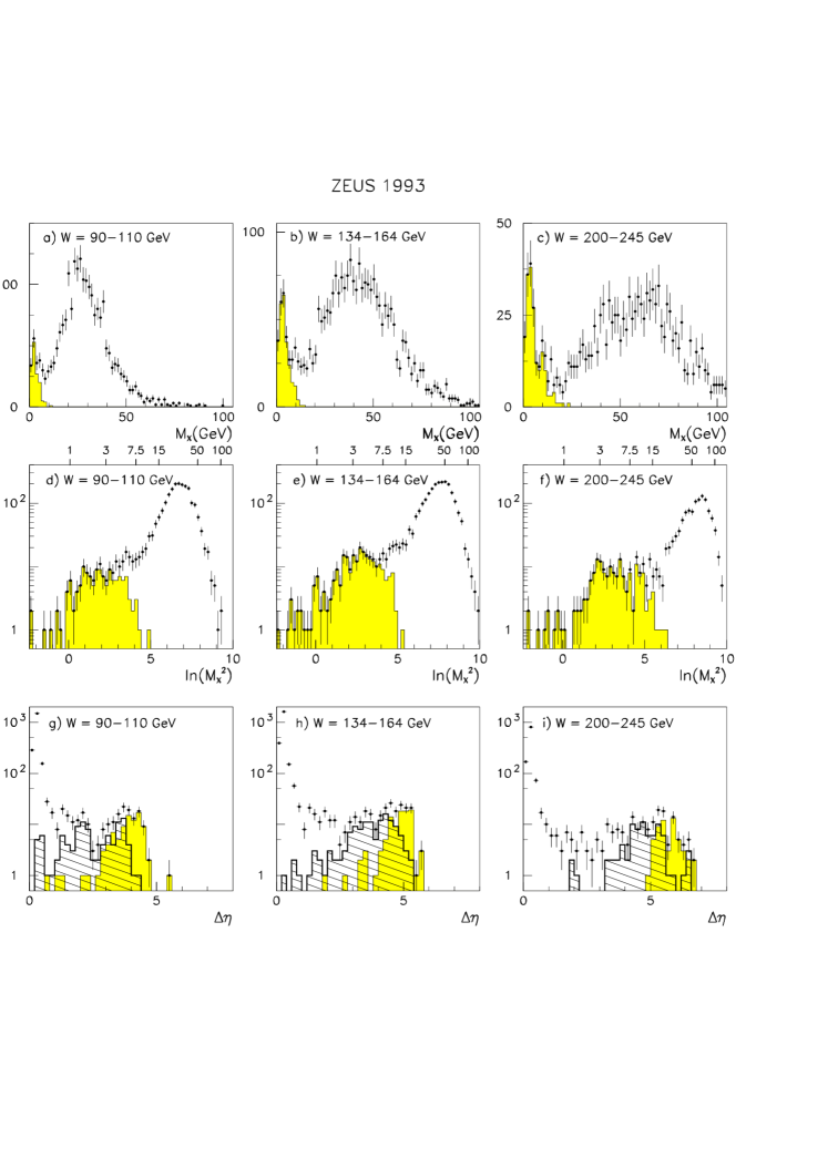
\begin{picture}(15.0,20.0)\end{picture}

Figure 6: Distributions of $M_{X}$ at $Q^{2}=$ 14 GeV²: a) - c) for the $W$ intervals 90 - 110, 134 - 164, 200 - 245 GeV. d) - f) Distributions of $\ln M^{2}_{X}$ for the same $W$ intervals. The shaded histograms in a) - f) show the events which have $\eta_{max}<1.5$ corresponding to a rapidity gap in the detector larger than 2.2 units. g) - i) Distributions of the rapidity gap $\Delta\eta$ for the same $Q^{2}$ and $W$ values. The histograms show the distributions for events with $M_{X}<$ 3 GeV (shaded) and $M_{X}=$ 3-7.5 GeV (skewed hatched). Here $M_{X}$ is the corrected mass. The distributions are not corrected for acceptance effects.

The measured $M_{X}$ distributions are shown in Figs. 6(a-c) for three $W$ intervals, $W=90-110,134-164$ and $200-245$ GeV at $Q^{2}$ = 14 GeV². The distributions are not corrected for acceptance. For all $W$ bins two distinct groups of events are observed, one peaking at low $M_{X}$ values, the other at high $M_{X}$ values. While the position of the low mass peak is independent of $W$, the high mass peak moves to higher values as $W$ increases. As already seen, most events in the low mass peak possess a large rapidity gap. This is illustrated by the shaded histograms which represent the events with $\eta_{max}<1.5$.

The size of the rapidity gap, $\Delta\eta$, can be seen from Figs. 6(g - i) which show the distributions of the rapidity gap between the edge of the calorimeter ($\eta\approx 3.9$, which is the $\eta$ value of the geometric center of the HAC cells closest to the proton beam) and the most forward lying cell with energy deposition greater than 200 MeV (the threshold is reduced in comparison with the determination of $\eta_{max}$ because here single cells are considered instead of a group of cells). The plots give the distribution of all events (points with error bars) and those with $M_{X}<$ 3 GeV (shaded) and 3 - 7.5 GeV (skewed hatching). There is a strong concentration of events at small rapidities, $\Delta\eta$ $<1$, which stem from non diffractive processes. The distributions demonstrate that the majority of low $M_{X}$ events are associated with a large rapidity gap $\Delta\eta~{}>2$. The average rapidity gap increases with growing $W$. For a given $W$ value $\eta_{max}$ is correlated with the maximum possible $M_{X}$ value but does not allow the determination of $M_{X}$ uniquely because of fragmentation effects. Since our aim is the determination of the diffractive cross section as a function of $M_{X}$, the analysis was based on $M_{X}$ and not on $\eta_{max}$.

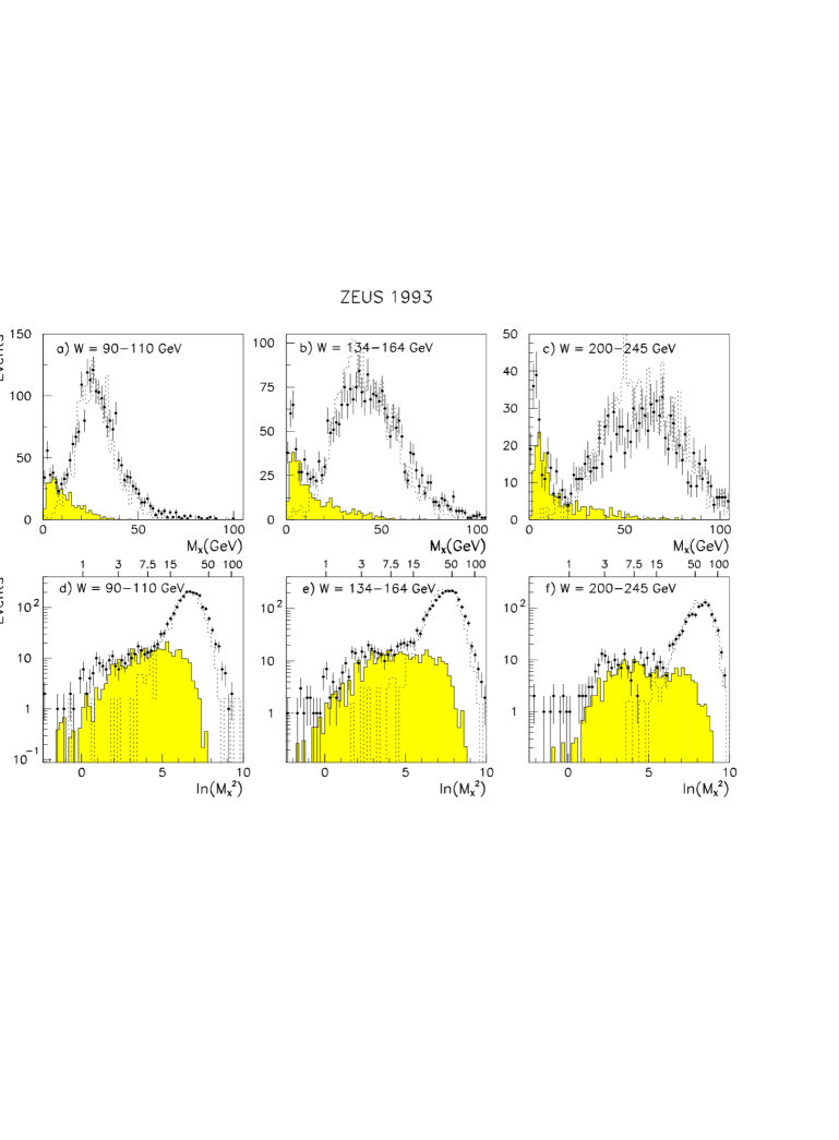
\begin{picture}(15.0,20.0)\end{picture}

Figure 7: Distributions of $M_{X}$ at $Q^{2}=$14 GeV²: a) - c) for the $W$ intervals 90 - 110, 134 - 164, 200 - 245 GeV, d) - f) plotted versus $\ln M^{2}_{X}$ for the same $W$ intervals as in a) - c). Here $M_{X}$ is the corrected mass. The distributions are not corrected for acceptance effects. Shaded histograms show the prediction of the NZ model for diffractive production; dashed histograms show the prediction of CDMBGF for nondiffractive production. The MC events were passed through the standard ZEUS detector simulation. The CDMBGF distributions were normalized to 85$\%$ of the data while the NZ distributions were normalized to the observed number of diffractive events with $M_{X}>$ 1.7 GeV; in the NZ model, diffractive events are generated for $M_{X}>$ 1.7 GeV.

In Fig. 7 the measured $M_{X}$ distributions are compared with the NZ and CDMBGF predictions. The shaded distributions show the NZ predictions for diffractive production. They peak at small masses. The predictions of CDMBGF for nondiffractive production (dotted histograms) peak at high masses. The sum of the NZ and CDMBGF contributions reproduce the main features of the data which are the low and high mass peaks.

The properties of the $M_{X}$ distributions can be understood best when plotted as a function of $\ln M_{X}^{2}$, shown in Figs. 6(d-f) and Figs. 7(d-f). Here, and in the following, masses and energies are given in units of GeV. In this representation the low mass peak shows up as a plateau-like structure at low $\ln M_{X}^{2}$, most notably at high $W$ values. The high mass peak exhibits a steep exponential fall-off towards smaller $\ln M_{X}^{2}$ values. The shape of the exponential fall-off is independent of $W$, a property which is best seen when the $\ln M_{X}^{2}$ distributions are replotted in terms of the scaled variable [$\ln M_{X}^{2}$ + $\ln(s/W^{2})$] (the total $ep$ c.m. energy squared, $s$, is introduced for convenience). This is shown in Fig. 8 at $Q^{2}=14$ and 31 GeV² where the scaled $\ln M_{X}^{2}$ distributions are overlaid for three $W$ intervals. The position of the high mass peak in $\ln M_{X}^{2}$ grows proportionally to $\ln W^{2}$ and the slope of the exponential fall-off towards small $\ln M_{X}^{2}$ values is approximately independent of $W$.

3.6 $M_{X}$ dependence of the nondiffractive contribution

While in diffractive scattering the outgoing nucleonic system remains colourless, in nondiffractive DIS the incident proton is broken up and the remnant of the proton is a coloured object. This gives rise to a substantial amount of initial and final state QCD radiation, followed by fragmentation, between the directions of the incident proton and the current jet as illustrated in Fig. 1. The salient features of the resulting $M_{X}$ distribution, namely the exponential fall-off and the scaling in [$\ln M_{X}^{2}$ + $\ln(s/W^{2})$], can be understood from the assumption of uniform, uncorrelated particle emission in rapidity ${\cal Y}$ along the beam axis in the $\gamma^{*}p$ system [37]:

$$dN_{part}/d{\cal Y}=\lambda,\;\;\;\;\lambda=\rm{constant.}$$ (13)

At the $Q^{2}$ values under study, for ${\cal Y}>0$, the beam axis in the $\gamma^{*}p$ system is approximately given by the proton direction in the HERA system. Since the shape of the rapidity distribution is invariant under translations along the $\gamma^{*}$ beam axis we translate the ${\cal Y}$ distribution measured in the $\gamma^{*}p$ system until the point of maximum rapidity agrees with the maximum rapidity ${\cal Y}_{max}$ in the $ep$ system. For an (idealized) uniform ${\cal Y}$ distribution between maximum and minimum rapidities of ${\cal Y}_{max}$ and ${\cal Y}_{min}$, respectively, the total center of mass energy $W$ is given by

$$W^{2}=c_{0}\cdot\exp({\cal Y}_{max}-{\cal Y}_{min}),\;\;\;{\rm{assuming}}\;\;\;({\cal Y}_{max}-{\cal Y}_{min})\gg 1.$$ (14)

Here, $c_{0}$ is a constant. The mass $M_{X}$ of the particle system that can be observed in the detector is reduced by particle loss mainly through the forward beam hole:

$$M_{X}^{2}=c_{0}\cdot\exp({\cal Y}^{det}_{limit}-{\cal Y}_{min})=W^{2}\cdot\exp({\cal Y}^{det}_{limit}-{\cal Y}_{max})$$ (15)

where ${\cal Y}^{det}_{limit}$ denotes the limit of the FCAL acceptance (neglecting the mass and transverse momentum of the produced particles). Equation 15 predicts scaling of the $\ln M^{2}_{X}$ distribution when plotted as a function of  $\ln(M^{2}_{X}/W^{2})$, in agreement with the behaviour of the data seen in Fig. 8 where the data are plotted in terms of [$\ln M^{2}_{X}+\ln(s/W^{2})$]. The quantity (${\cal Y}_{max}-{\cal Y}^{det}_{limit}$) is the effective width of the beam hole and can be estimated from the effective maximum rapidity and the detector geometry.

The mass $M_{X}$ is expected to fluctuate statistically due to a finite probability $P(0)$ that no particles are emitted between ${\cal Y}^{det}_{limit}$ and ${\cal Y}^{det}_{limit}-\Delta{\cal Y}$. This generates a gap of size $\Delta{\cal Y}$. The assumption of uncorrelated particle emission leads to Poisson statistics which predicts $P(0)=exp(-\lambda\Delta{\cal Y})$ resulting in an exponential fall-off of the $\ln M^{2}_{X}$ distribution,

$$\frac{d{\cal N}^{nondiff}}{d\ln M^{2}_{X}}=c\,\exp(b\ln M^{2}_{X})\;\;\;,$$ (16)

where the slope $b$ is equal to the parameter $\lambda$ and $c$ is a constant. The exponential fall-off of the $\ln M_{X}^{2}$ distribution towards small values of $\ln M^{2}_{X}$ expected from this simplified consideration is indeed observed in models which include QCD leading order matrix elements, parton showers and fragmentation such as CDMBGF shown by the dashed histograms in Figs. 7(d-f). This shows that the known sources of long range correlations like conservation of energy and momentum, of charge and of colour, which are incorporated in CDMBGF, do not lead to significant deviations from an exponential behaviour with the possible exception of a very small fraction ($0.2-0.4\%$) of the CDMBGF events which is found above the exponential at low $\ln M^{2}_{X}$ values.

In principle, the exponential fall-off of the $\ln M_{X}^{2}$ distribution should start at the maximum value of $\ln M_{X}^{2}$ allowed by kinematics and acceptance, Max$(\ln M_{X}^{2})=\ln W^{2}-(2$ to $3)$. The data in Fig. 6d-f and Fig. 8 break away from the exponential behaviour towards high values of $\ln M_{X}^{2}$ leading to a rounding-off. It mainly results from the finite size of the selected $W$ intervals, the edge of the calorimeter acceptance in the forward direction ($\eta_{edge}$ = 3.7 to 4.3) and the finite resolutions with which $W$ and $M_{X}$ are measured. With good accuracy the exponential fall-off is observed for $\ln M_{X}^{2}\leq\ln W^{2}-\eta_{0}$, with $\eta_{0}\approx 3.0$, over more than two units of rapidity (see also Section 4.2).

We would like to add three remarks. Firstly, the value of the slope $b$ is little affected by detector effects: it is almost the same at the detector level as at the generator level. This was verified by Monte Carlo simulation of nondiffractive events with CDMBGF. The MC events were selected using the same selection cuts as for the data. The mass $M_{X}$ of a standard nondiffractive DIS event at the generator level was defined as the invariant mass of all particles (excluding the scattered electron) generated with pseudorapidities $\eta<4.3$, the nominal end of the detector. In Fig. 9 the MC generated (dashed histograms) and MC measured mass distributions (solid histograms) are shown. The exponential slope values of $b=1.9\pm 0.1$ (shown as straight lines) obtained at the generator level agree with the slope values found at the detector level to within $\pm 0.1$ units compatible with the statistical errors of the simulation.

Secondly, the value predicted by CDMBGF for the slope is $b=1.9\pm 0.1$ while the data yield a shallower slope, the average being $\overline{b}=1.46\pm 0.15$. Note, the value of the slope $b$ cannot be predicted precisely by the models; rather, DIS data have to be used to fix the relevant parameters of the CDMBGF model. For instance, short range correlations arising from resonance production affect the value of $b$. The observed difference between the exponential fall-off found in the data and predicted by the Monte Carlo simulation indicates that estimating the tail of the nondiffractive background from Monte Carlo simulation alone may lead to an incorrect result for the diffractive cross section.

Thirdly, we determine the slope $b$ from the data in a region where the nondiffractive contribution dominates. The exponential fall-off will be assumed to continue with the same slope into the region of overlap with the diffractive contribution. The nondiffractive event sample generated with CDMBGF indicates a small excess of events above the exponential fall-off (see above). If allowance is made for a similar deviation from the exponential fall-off in the data, the numbers of diffractive events obtained after subtraction of the nondiffractive background change by less than $\approx 30\%$ of their statistical error.

3.7 $M_{X}$ dependence of the diffractive contribution

In diffractive events, the system $X$ resulting from the dissociation of the photon is, in general, almost fully contained in the detector while the outgoing proton or low mass nucleonic system, $N^{dissoc}$, escapes through the forward beam hole. Furthermore, diffractive dissociation prefers small $M_{X}$ values and leads to an event distribution of the form $d{\cal N}/dM_{X}^{2}\propto 1/(M_{X}^{2})^{(1+n)}$ or

$$\frac{d{\cal N}}{d\ln M_{X}^{2}}\sim\frac{1}{(M_{X}^{2})^{n}},$$ (17)

approximately independent of $W$. At high energies and for large $M_{X}$ one expects $n\approx 0$ leading to a roughly constant distribution in $\ln M^{2}_{X}$. Such a mass dependence is seen in diffractive dissociation of $pp$ scattering (see e.g. [12, 13]). A value of $n\approx 0$ is also expected in diffractive models as the limiting value for the fall-off of the mass distribution (see e.g. the NZ model [31]).

To summarize this and the previous section, the diffractive contribution is identified as the excess of events at small $M_{X}$ above the exponential fall-off of the nondiffractive contribution with $\ln M^{2}_{X}$. The exponential fall-off permits the subtraction of the nondiffractive contribution and therefore the extraction of the diffractive contribution without assuming the precise $M_{X}$ dependence of the latter. The $M_{X}$ distribution is expected to be of the form

$$\frac{d{\cal N}}{d\,\ln M_{X}^{2}}=D+c\,\exp(b\,\ln{M_{X}^{2}}),~{}~{}~{}~{}{\rm for}~{}~{}~{}\ln M_{X}^{2}\leq\ln W^{2}-\eta_{0}.$$ (18)

Here, $D$ denotes the diffractive contribution, the second term represents the nondiffractive contribution and $\ln W^{2}-\eta_{0}$ is the maximum value of $\ln M^{2}_{X}$ up to which the exponential behaviour of the nondiffractive part holds. We shall apply Eq. 18 in a limited range of $\ln M^{2}_{X}$ for fitting the parameters $b,c$ of the nondiffractive contribution. The diffractive contribution will not be taken from the fit result for $D$ but will be determined by subtracting from the observed number of events the nondiffractive contribution found in the fits.

3.8 Contribution from nucleon dissociation

The contribution from the diffractive process where the nucleon dissociates,

$$ep\to e+X+N^{dissoc},$$

was estimated by Monte Carlo simulation. Assuming factorisation and a Triple Regge formalism  [35, 36] for modelling $\gamma^{*}p\to X+p$ and $\gamma^{*}p\to X+N^{dissoc}$, the measured cross sections for elastic and single diffractive dissociation in $pp$ (and $\overline{p}p$) scattering, $pp\to p+p$ and $pp\to p+N^{dissoc}$, were used to relate $\gamma^{*}p\to X+N^{dissoc}$ to $\gamma^{*}p\to X+p$.

The secondary particles from $N^{dissoc}$ decay were found to be strongly collimated around the direction of the proton beam. Analysis of the angular distribution of the secondary particles as a function of $M_{N}$ showed that for $M_{N}<2$ GeV basically no energy is deposited in the calorimeter while for events with $M_{N}>6$ GeV there are almost always secondaries which deposit energy in the calorimeter. Furthermore, events of the type $ep\to e+X+N^{dissoc}$, where decay particles from $N^{dissoc}$ deposit energy in the calorimeter, have in general a mass reconstructed from all energy deposits in the calorimeter (including those from the decay of the system $X$ but excluding those of the scattered electron) which is much larger than the mass of $X$. As a result these events make only a small contribution to the event sample selected below for diffractive production of $\gamma^{*}p\to X+N$ either with $M_{X}<7.5$ GeV or $M_{X}<15$ GeV. To a good approximation, the selection includes all events from dissociation of the nucleon, $\gamma^{*}p\to X+N^{dissoc}$, with $M_{N}<4$ GeV. From the comparison with the $pp$ data, we estimate the contribution of $\gamma^{*}p\to X+N^{dissoc}$ with $M_{N}<4$ GeV to the diffractive sample to be $11\pm 5\%$.

4 Extraction of the diffractive contribution

4.1 Binning in $Q^{2}$ and $W$

The cross section for $\gamma^{*}p\to X+N$ was determined for two $Q^{2}$ intervals, $10$ - $20$ GeV² and $20$ - $56$ GeV², the average values being 14 GeV² and 31 GeV², respectively. This choice of $Q^{2}$ intervals was motivated by the available event statistics and by the requirement of good acceptance. These requirements also determined the $W$ range of $60<W<245$ GeV. The intervals in $W$ were chosen so as to have equidistant bins in $\ln W^{2}$ providing approximately equal numbers of events in each $W$ bin. For the bin width, $\Delta$ $\ln W^{2}$ = 0.4 was used, commensurate with the resolution for $\ln W^{2}$ of 0.17 for diffractive events and 0.32 for nondiffractive events, as determined by Monte Carlo simulation. The better resolution for diffractive events is due to the fact that here the decay particles from the system $X$ are almost completely contained in the detector.

The total number of accepted events in the region $60<W<245$ GeV and $10<Q^{2}<20\,{\rm GeV}^{2}$ ($20<Q^{2}<56\,{\rm GeV}^{2}$) was 14466 (11247).

4.2 Fitting the nondiffractive contribution

The mass distributions for all $W$ and $Q^{2}$ intervals are presented in Figs. 10 - 11 in terms of $\ln M_{X}^{2}$. The diffractive contribution was obtained for each $W,Q^{2}$ interval by determining first the nondiffractive background from a fit to the data at large $\ln M^{2}_{X}$. The nondiffractive background was then extrapolated to the small $\ln M^{2}_{X}$ region and subtracted from the data giving the diffractive contribution as illustrated in Fig. 12. The fit for the nondiffractive background was performed using Eq. 18. The diffractive contribution $D$ was assumed to be of the form

$$\frac{d{\cal N}^{diff}}{d\,\ln M_{X}^{2}}=D_{1}\;+\;\frac{D_{2}}{M^{2}_{X}}.$$ (19)

where $D_{1}$ and $D_{2}$ are constants. The second term allows for contributions from lower lying Regge poles contributing to $\gamma^{*}$ pomeron scattering at a c.m. energy of $M_{X}$ or from a hard quark distribution in the pomeron (e.g. Hard POMPYT). The fit parameters are $D_{1}$, $D_{2}$, $b$ and $c$.

The fits were performed to the data in the range $\ln Q^{2}<\ln M^{2}_{X}<{\rm Max}(\ln M^{2}_{X})$. The lower limit for $\ln M^{2}_{X}$ was chosen according to the expectation of the diffraction models  [29, 31, 38], that for $M^{2}_{X}>Q^{2}$ the diffractive contribution is of the form given by Eq. 19. The upper limit Max$(\ln M^{2}_{X})$ was chosen as the maximum value of $\ln M^{2}_{X}$ up to which the data exhibit an exponential behaviour. The maximum value of $\ln M^{2}_{X}$ was determined by fitting the $\ln M^{2}_{X}$ distributions for each ($W,Q^{2}$) interval with a varying maximum value of $\ln M^{2}_{X}$. In most ($W,Q^{2}$) intervals a clear boundary as a function of Max$(\ln M^{2}_{X})$ was observed beyond which the $\chi^{2}$ probability for the fit dropped rapidly. The boundary marks the location where the distribution starts to deviate from an exponential behaviour. The boundary was found to be at $\ln M^{2}_{X}+\ln(s/W^{2})=8.8$ corresponding to a value of $\eta_{0}=3.0$, a value which is in good agreement with expectations of $\eta_{0}$ = ${\cal Y}_{max}-{\cal Y}^{det}_{limit}$ (see discussion above). The fits were performed with Max$(\ln M^{2}_{X})=\ln(W^{2}/s)+8.6$. In the studies of systematic uncertainties the maximum value was increased (decreased) by 0.2 (0.4), see section 5.2. The $\chi^{2}$ probabilities for the fits were on average 40$\%$.

The fits were performed by including both terms, $D_{1}$ and $D_{2}$, (extended fits) as well as by assuming $D_{2}=0$ (nominal fits). Since the two fit procedures resulted in only minor differences we used the results from the nominal fits and used those from the extended fits for estimating the systematic errors (see section 5.2). The solid lines in Figs. 10 - 11 show for all $Q^{2}$ and $W$ bins the exponential fall-off of the nondiffractive contribution resulting from the fits. The nondiffractive contribution moves to larger $\ln M^{2}_{X}$ values proportional to $\ln W^{2}$. As $W$ increases, the diffractive contribution appears with little background over an increasing $M_{X}$ range. Above $W=90~{}(164)$ GeV the nondiffractive background is small up to $M_{X}$ values of 7.5 (15) GeV (see also Table 1 below).

In Figs. 10 and 11 the nondiffractive background estimates are also compared with the predictions of the CDMBGF simulation. The dotted histograms display the predictions of CDMBGF for the nondiffractive contribution normalized to 85$\%$ of the number of events observed in the data in each ($W,Q^{2}$) bin, the 15% reduction accounting roughly for the diffractive contribution. The qualitative features of the data are reproduced by CDMBGF in all $Q^{2}$ and $W$ intervals, although the exponential slopes are steeper than in the data (see discussion in section 3.6).

5 Determination of the diffractive cross section

The number of diffractive events, ${\cal N}^{diff}_{meas}$, was determined in all $Q^{2}$ and $W$ bins for the $M_{X}$ intervals $<3$ GeV ($\ln M_{X}^{2}<2.2$), $3-7.5$ GeV ($\ln M_{X}^{2}=2.2-4.0$) and $7.5-15$ GeV ($\ln M_{X}^{2}=4.0-5.4$) by subtracting from the observed number of events, ${\cal N}_{obs}$, the contribution from electron beam gas scattering, ${\cal N}^{egas}$, and the nondiffractive contribution, ${\cal N}^{nondiff}$, obtained from the fit, ${\cal N}^{diff}_{meas}={\cal N}_{obs}-{\cal N}^{egas}-{\cal N}^{nondiff}$. Electron-gas scattering produces low $M_{X}$ events, which are candidates for diffractive scattering; most of them have no reconstructed vertex. Events from unpaired electron bunches were used to obtain ${\cal N}^{egas}$.

From ${\cal N}^{diff}_{meas}$ the number of produced diffractive events, ${\cal N}^{diff}_{prod}$, was obtained by a Bayesian unfolding procedure which took into account detector effects such as bin-to-bin migration, trigger biases and event selection cuts. In the unfolding, the event distribution generated by Monte Carlo, $n_{G}(i)$, was reweighted as discussed in section 3.2 so that the observed Monte Carlo distribution, $n_{O}(j)$, reproduced closely ${\cal N}^{diff}_{meas}$, the event distribution measured in the data which will be denoted by $n_{Dat}(j)$. The indices $i,j$ denote the three - dimensional bins in ($M_{X}$, $W$, $Q^{2}$) in which the data were analyzed. For every set of weights we determined from the generated distribution the observed distribution and the transfer matrix $T_{GO}(j,i)$, which leads from the observed to the generated distribution, $n_{G}(i)=\sum_{j}T_{GO}(j,i)n_{O}(j)$. In an iterative procedure the $\chi^{2}$ obtained from the differences of $n_{Dat}(j)$ and $n_{O}(j)$ was minimized by varying the weighting parameters of the TRM function given in Eq. 12. A good description of the data was obtained; the minimum $\chi^{2}=34$ for $28$ degrees of freedom. The values found for the weighting parameters were $c_{L}=0.1$, $M_{0}/Q=1$ and $\overline{\mbox{$\alpha_{{}_{IP}}$}}=1.2$. The resulting matrix $T_{GO}(j,i)$ was then used to determine the unfolded event distribution from that measured, $n_{U}(i)=\sum_{j}T_{GO}(j,i)n_{Dat}(j)$. The number of unfolded events is denoted by ${\cal N}^{diff}_{prod}$. In the calculation of the statistical errors, the bin-to-bin correlations were neglected. The errors were checked by examining the spread of results obtained by dividing the data into several subsamples.

5.1 Evaluation of the cross sections

For the final analysis, only bins where the fraction of nondiffractive background was less than 50 $\%$ and the purity was above 30 $\%$ were kept. Purity is defined as the ratio of the number of events generated in the bin and observed in the same bin divided by the total number of events observed in the bin. The average purity in a ($M_{X},W,Q^{2}$) bin was 43 $\%$.

Electromagnetic radiative effects were corrected for in every ($M_{X},W,Q^{2}$) bin [39]. The corrections were less than $10\%$ and independent of $W$.

The average differential cross section for $ep$ scattering, in a ($M_{X},W,Q^{2}$) bin, is obtained by dividing the number of unfolded events, ${\cal N}^{diff}_{prod}$, by the luminosity and the bin widths. The lower limit of $M_{X}$, was taken to be 2$m_{\pi}$, where $m_{\pi}$ is the pion mass.

The cross sections for the process $ep\to eXN$ can be expressed in terms of the transverse (T) and longitudinal (L) cross sections $\sigma_{T}^{diff}$, $\sigma_{L}^{diff}$, for $\gamma^{*}p\to XN$ as follows [40]:

$$Q^{2}\,\frac{d\sigma^{diff}_{ep\to eXN}(M_{X},W,Q^{2})}{dM_{X}d\ln W^{2}dQ^{2}}=\frac{\alpha}{2\pi}\,[(1-y)^{2}+1][\sigma_{T}^{diff}+\sigma_{L}^{diff}][1-\frac{y^{2}}{(1-y)^{2}+1}\frac{\sigma_{L}^{diff}}{\sigma_{T}^{diff}+\sigma_{L}^{diff}}].$$ (20)

The relative contribution of the correction term in the third square bracket on the r.h.s. of Eq. 20 is negligible if $y\ll 1$ or $\sigma^{diff}_{L}\ll\sigma^{diff}_{T}$. Since $y\approx W^{2}/s$, the contribution can be substantial only at high $W$ values. In the extreme case that $\sigma^{diff}_{L}\gg\sigma^{diff}_{T}$, the correction term will increase $[\sigma^{diff}_{T}+\sigma^{diff}_{L}]$ by at most $35\%$ for the highest $W$ bin ($200-245$ GeV) and $11\%$ for the next highest $W$ bin (164 - 200 GeV). If $\sigma^{diff}_{L}=Q^{2}/M^{2}_{X}\cdot\sigma^{diff}_{T}$, as e.g. in the Vector Dominance Model or in partonic models (see e.g. [41]), then the second term increases $[\sigma^{diff}_{T}+\sigma^{diff}_{L}]$ by at most $31\%$ ($17\%,6\%$) for the bins with the highest $W$, $Q^{2}$ values and $M_{X}<3$ GeV ($3-7.5$ GeV, $7.5-15$ GeV) falling below $10\%$ ($6\%,2\%$) in the next highest $W$ bin .

In the following analysis, the correction term was set equal to one:

$$\frac{d\sigma^{diff}_{\gamma^{*}p\to XN}(M_{X},W,Q^{2})}{dM_{X}}\equiv\frac{d(\sigma_{T}^{diff}+\sigma_{L}^{diff})}{dM_{X}}\approx\frac{2\pi}{\alpha}\,\frac{Q^{2}}{(1-y)^{2}+1}\,\frac{d\sigma^{diff}_{ep\to eXN}(M_{X},W,Q^{2})}{dM_{X}d\ln W^{2}dQ^{2}}\;.$$ (21)

The numbers of events observed and estimated to come from background are given in Table 1, together with the values of the $\gamma^{*}p\to XN$ differential cross sections averaged over the specified $M_{X}$ range. The cross sections are quoted for the $Q^{2}$ values of 14 and 31 GeV² and the $W$ values corresponding to the logarithmic means of the $W$ interval limits. The average $M_{X}$ values in each $M_{X}$ interval are 1.9, 5.1, 11.0 GeV at $Q^{2}=14$ GeV² and 2.0, 5.1 and 11.0 GeV at $Q^{2}=31$ GeV².

5.2 Systematic errors

The systematic errors on the cross sections were estimated by varying the cuts and algorithms used to select the events. The bin-by-bin changes from the standard values were recorded. For reference each test is numbered; the number is given in brackets {}.

The efficiency for finding the scattered electron was around $100\%$ for $E^{\prime}_{e}>18$ GeV, falling to $55\%$ at $E^{\prime}_{e}=10$ GeV. To evaluate the resulting uncertainty on the cross section the cut on $E^{\prime}_{e}$ was raised {1} (lowered {2}) from 8 to 10 GeV (7 GeV); the box cut was varied from 32 cm to 36 cm {3} (28 cm {4}). The changes on the measured cross sections were negligible except for one low $W$ bin where a $28\%$ change of the cross section was observed.

In order to test for remaining background from photoproduction and for the sensitivity to radiative effects, which were not simulated in the diffractive Monte Carlo, the cut on $\sum_{h}(E-p_{Z})$ was raised {5} (lowered {6}) from $35$ GeV to $38$ GeV ($32$ GeV). This resulted in small changes of the cross sections, except in one bin where it reached $20\%$.

The effect of the cut on $y_{JB}$ was tested by raising {7} (lowering {8}) it from $0.02$ to $0.03$ ($0.01$). The changes were found to be below $5\%$, except for the low $M_{X}$ interval where in two low $W$ bins the higher $y_{JB}$ cut substantially reduced the acceptance; for these bins changes of $19\%$ and $47\%$, respectively, were observed.

The mass correction factor was assumed to be different by +10$\%$ {9} (-10$\%$ {10}) in the Monte Carlo simulation and in the data. This affected the low $W$ bins where changes up to $17\%$ were observed.

The analysis was performed without requiring a reconstructed event vertex and could therefore be affected by background from beam-gas scattering. The analysis was repeated requiring an event vertex as determined by tracking where the Z-coordinate of the vertex had to lie in the interval -50 cm to +40 cm {11}. This requirement was satisfied by $89\%$ of the accepted events. The vertex requirement reduced the total number of events in the accepted ($M_{X}$,$W$,$Q^{2}$) bins obtained with unpaired electron bunches from 12 to 1 event thereby suppressing the electron-gas background to a negligible amount. Apart from this effect reductions of the cross sections by at most $12(16)\%$ in the highest $W$ bins at $Q^{2}=14(31)~{}$GeV² were observed. For the other bins the changes were smaller.

Uncertainties in the number of diffractive events resulting from the subtraction of the nondiffractive background were estimated by increasing {12} (decreasing {13}) the upper limit of the fit range in $\ln M^{2}_{X}$ by 0.2 (0.4) units; by decreasing the lower limit of the fit range in $\ln M^{2}_{X}$ by 0.4 units {14}; by repeating the fits for the nondiffractive background with the extended form Eq. 19, $D_{2}~{}\neq~{}0$, for the diffractive part {15}. The typical changes were below 10$\%$. The largest change was observed for the lowest $W$ bin at $Q^{2}=31$ GeV² where it reached $37\%$.

The uncertainty resulting from the Monte Carlo weighting procedure was estimated by varying the weighting parameter $\overline{\mbox{$\alpha_{{}_{IP}}$}}$ from 1.2 to 1.1 {16} and 1.3 {17}. To estimate the uncertainty of the Monte Carlo modelling for the low $M_{X}$ region the $\rho^{o}$ events for $M_{X}<1$ GeV were replaced by a system decaying into $\pi^{+}$, $\pi^{-}$, $\pi^{o}$’s with a phase space like distribution. Changes of less than $8\%$ were observed.

The total systematic error for each bin was determined by adding quadratically the individual systematic uncertainties, separately for the positive and negative contributions. The total errors were obtained by adding the statistical and systematic errors in quadrature. The errors do not include an overall normalization uncertainty of 3.5$\%$ of which 3.3$\%$ is from the luminosity determination and 1$\%$ from the uncertainty in the trigger efficiency.

6 Differential cross section for $\gamma^{*}p\to X+N$

The differential cross section $d\sigma^{diff}_{\gamma^{*}p\to XN}/dM_{X}$ was determined according to Eq.(21) for the different ($M_{X}$,$W$,$Q^{2}$) intervals. The results are shown in Fig. 13, as a function of $W$ averaged over the $M_{X}$ bins $2m_{\pi}$ - 3 GeV, 3 - 7.5 GeV and 7.5 - 15 GeV at $Q^{2}=14$ and $31$ GeV². The solid points show the measured values. The inner error bars give the statistical errors. For the full bars the statistical and systematic errors have been added in quadrature.

The cross section, within errors, is seen to rise linearly with $W$ at both $Q^{2}$ values for all $M_{X}$ bins up to 7.5 GeV. For the $M_{X}$ bins (7.5 - 15) GeV the data in the accepted $W$ range are consistent with this rise.

In a Regge - type description  [35, 36], the $W$ dependence of the diffractive cross section is of the form

$$\frac{d\sigma^{diff}_{\gamma^{*}p\to XN}(M_{X},W,Q^{2},t)}{dtdM_{X}} \propto(W^{2})^{2\mbox{$\alpha_{{}_{IP}}$}(0)-2}\;\cdot\;e^{t(B+2\mbox{$\alpha_{{}_{IP}}$}^{\prime}\ln(W^{2}/(M_{X}^{2}+Q^{2}))}\;\;\;,$$ (22)

where $\mbox{$\alpha_{{}_{IP}}$}(t)$ = $\mbox{$\alpha_{{}_{IP}}$}(0)$ + $\mbox{$\alpha_{{}_{IP}}$}^{\prime}t$ is the pomeron trajectory and $B$ and $\mbox{$\alpha_{{}_{IP}}$}^{\prime}$ are parameters. The cross sections in each ($M_{X}$, $Q^{2}$) interval were fitted to the form

$$\frac{d\sigma^{diff}_{\gamma^{*}p\to XN}(M_{X},W,Q^{2})}{dM_{X}} \propto(W^{2})^{(2\overline{\mbox{$\alpha_{{}_{IP}}$}}-2)}\;\;\;,$$ (23)

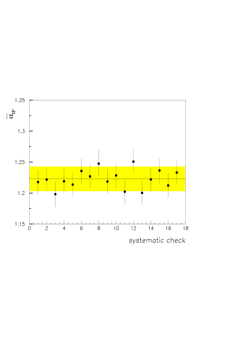
\begin{picture}(15.0,20.0)\end{picture}

Figure 14: Sensitivity of the value of $\overline{\mbox{$\alpha_{{}_{IP}}$}}$ to the different sources of systematic uncertainties. The central line and the shaded band show for the standard fit the value of $\overline{\mbox{$\alpha_{{}_{IP}}$}}$ and $\pm$ 1 s.d. The dots give the $\overline{\mbox{$\alpha_{{}_{IP}}$}}$ value with its uncertainty obtained by repeating the analysis for each systematic check labeled 1 through 17 as described in the text.

where $\overline{\mbox{$\alpha_{{}_{IP}}$}}$ stands for $\mbox{$\alpha_{{}_{IP}}$}(t)$ averaged over the $t$ distribution. The fit was performed by considering $\overline{\mbox{$\alpha_{{}_{IP}}$}}$ and the six normalization constants for the six ($M_{X}$, $Q^{2}$) intervals as free parameters. Taking into account only the statistical errors, $\overline{\mbox{$\alpha_{{}_{IP}}$}}$ was found to be $1.23\pm 0.02$ with $\chi^{2}/ndf=11.7/24$. The systematic uncertainties were estimated by repeating the fit independently for every source of systematic error discussed above. The results are shown in Fig. 14. The lowest $\overline{\mbox{$\alpha_{{}_{IP}}$}}$ value obtained was 1.20, the highest value was 1.25. The observed deviations were added in quadrature leading to the final value:

$$\overline{\mbox{$\alpha_{{}_{IP}}$}}\;\;=\;\;1.23\pm 0.02(stat)\pm 0.04(syst).$$

The $W$ dependence was also determined by restricting the analysis to those ($M_{X}$,$W$,$Q^{2}$) bins where almost all events have a large rapidity gap and where, therefore, nondiffractive contributions should be negligible. Of the events observed with $M_{X}<$ 3 GeV, 98$\%$ have a rapidity gap $\Delta\eta>$ 2. The fit to these events yielded $\overline{\mbox{$\alpha_{{}_{IP}}$}}=$ 1.24 $\pm~{}0.03~{}^{+0.07}_{-0.03}$. Note that the average rapidity gap for these events grows with $W$ and a possible background from nondiffractive scattering would diminish with rising $W$. Consequently, if there were a nondiffractive contribution left in the sample, the correction for this background would lead to an increase of the value of $\overline{\mbox{$\alpha_{{}_{IP}}$}}$ compared to the result obtained.

The effect of the kinematically allowed minimum value of $|t|$ ($|t|_{min}$) on the $t$ - integrated cross section and therefore on the value of $\overline{\mbox{$\alpha_{{}_{IP}}$}}$ is negligible, $|t|_{min}$ being less than $10^{-3}$ GeV². If $\mbox{$\alpha_{{}_{IP}}$}^{\prime}=0$ then $\overline{\mbox{$\alpha_{{}_{IP}}$}}$ is equal to the pomeron intercept at $t=0$, $\mbox{$\alpha_{{}_{IP}}$}(0)=\overline{\mbox{$\alpha_{{}_{IP}}$}}$. If the slope $\mbox{$\alpha_{{}_{IP}}$}^{\prime}$ in diffractive DIS is the same as for the soft pomeron ($\mbox{$\alpha_{{}_{IP}}$}^{\prime}=0.25$ GeV^-2) and the parameter $B$ is equal to half the value observed for elastic $pp$ scattering [12] ($B=4.5$ GeV^-2), then $\mbox{$\alpha_{{}_{IP}}$}(0)$ will increase from 1.23 to 1.26. Our result can be compared with the soft pomeron trajectory [11], $\mbox{$\alpha_{{}_{IP}}$}(t)=1.08+0.25t$, as determined from hadron - hadron scattering. Assuming $B=$ 4.5 GeV^-2 and averaging over $t$, the soft pomeron predicts $\overline{\mbox{$\alpha_{{}_{IP}}$}}=1.05$. In extracting the diffractive cross section, the assumption $\sigma^{diff}_{L}=0$ was made. Assuming instead $\sigma^{diff}_{L}=(Q^{2}/M^{2}_{X})\sigma^{diff}_{T}$ (see for example [41]) will increase $\overline{\mbox{$\alpha_{{}_{IP}}$}}$ from 1.23 to 1.28. Hence, a positive slope of the pomeron trajectory and/or a finite $\sigma^{diff}_{L}$ contribution will lead to a larger $\mbox{$\alpha_{{}_{IP}}$}(0)$ value and increase the difference with respect to the soft pomeron intercept.

The observation of $\overline{\mbox{$\alpha_{{}_{IP}}$}}$ being substantially larger in diffractive DIS than expected for the soft pomeron is in line with the expectation of perturbative QCD  [14] and shows that deep inelastic diffractive scattering has a perturbative contribution. The measured value of $\overline{\mbox{$\alpha_{{}_{IP}}$}}$ is smaller than the value which would follow from the BFKL formalism, $\mbox{$\alpha_{{}_{IP}}$}(0)\approx 1.5$. It is in broad agreement with the effective pomeron intercept expected in the perturbative models of  [42, 43] where the Bjorken-$x$ dependence of the gluon momentum density $xg(x,Q^{2})$ of the proton determines the $W$ dependence of diffractive scattering.

There are also models where the effective $\mbox{$\alpha_{{}_{IP}}$}(0)$ is expected to be smaller in diffractive hadron - hadron or photon - hadron scattering as compared to deep inelastic diffractive scattering because in hadron - hadron or photoproduction processes, in addition to single, multiple pomeron exchanges also contribute (see e.g. [44]). In these models the importance of multiple pomeron exchanges decreases quickly with growing photon virtuality.

6.1 Diffractive contribution to total deep inelastic scattering

The relative contribution of diffractive scattering to the total virtual-photon proton cross section, $\sigma^{tot}_{\gamma^{*}p}$, was determined for the $W$ bin (164 - 200 GeV) where data on the diffractive cross section are available up to $M_{X}=15$ GeV. The data for $\sigma^{tot}_{\gamma^{*}p}$ were taken from the analysis of the proton structure function $F_{2}$ [19]. The ratio $r^{diff}=\int dM_{X}\sigma^{diff}_{\gamma^{*}p\to XN}(M_{N}<4~{}{\rm GeV})/\sigma^{tot}_{\gamma^{*}p}$ is given in Table 2 integrated over different $M_{X}$ bins at $Q^{2}=14$ and $31$ GeV². In the lowest $M_{X}$ bin the relative contribution from diffractive scattering to the total DIS drops by a factor of about three from $Q^{2}=14$ to $31$ GeV². With increasing $M_{X}$ the relative contributions from diffractive scattering tend to become equal for the two values of $Q^{2}$. The observed $Q^{2}$ behaviour does not preclude a leading twist behaviour of the diffractive DIS cross section (observed by [1, 4]): the measurements for the two different $Q^{2}$ values correspond to different values of $x$, namely $x=Q^{2}/W^{2}=4\cdot 10^{-4}$ and $9\cdot 10^{-4}$, respectively. Furthermore, it is conceivable that for fixed $x$ the $Q^{2}$ behaviour of the diffractive cross section changes with $M_{X}$ and only its integral over $M_{X}$ is of leading twist [45].

7 Diffractive structure function of the proton

The DIS diffractive cross section, $ep\to e+X+N$, can be expressed in terms of the diffractive structure function $F^{D(3)}_{2}(\beta,Q^{2},\mbox{$x_{{}_{IP}}$})$ as follows [46]:

$$\frac{d\sigma^{diff}_{ep\to eXN}(\beta,Q^{2},\mbox{$x_{{}_{IP}}$},M_{N}<4\,{\rm GeV})}{d\beta dQ^{2}d\mbox{$x_{{}_{IP}}$}} = \frac{2\pi\alpha^{2}}{\beta Q^{4}}[1+(1-y)^{2}]F^{D(3)}_{2}(\beta,Q^{2},\mbox{$x_{{}_{IP}}$})$$ (24)

if the contribution from longitudinal photons is neglected.

In Fig. 15 we show $F^{D(3)}_{2}$ of this analysis as calculated from the differential cross sections $d\sigma^{diff}_{\gamma^{*}p\to XN}/dM_{X}$, $M_{N}<$ 4 GeV. The result is plotted as a function of $x_{{}_{IP}}$ for different values of $\beta$ and $Q^{2}$ (solid points). The error bars show the statistical and systematic errors added in quadrature. The data from our previous analysis [6] of $F^{D(3)}_{2}$ are also shown as the open points. In the previous analysis, the diffractive contribution was determined with a rapidity gap method using CDMBGF to estimate the nondiffractive part. Note that these data have been evaluated at somewhat different $\beta$ and $Q^{2}$ values than in the present analysis.

The diffractive structure function falls rapidly with increasing $x_{{}_{IP}}$, the $x_{{}_{IP}}$ dependence being the same within errors in all $\beta$ and $Q^{2}$ intervals. A good fit to the data from this analysis (solid points) is obtained with the form $F^{D(3)}_{2}=constant\cdot(1/\mbox{$x_{{}_{IP}}$})^{a}$ yielding $a=1.46\pm 0.04(stat)\pm 0.08(syst)$. Note, for fixed $Q^{2}$ and $\beta$ the $x_{{}_{IP}}$ dependence of $F^{D(3)}_{2}$ is equivalent to the $W$ dependence of $d\sigma^{diff}(\gamma^{*}p\to XN)/dM_{X}$ discussed above, the values of $a$ and $\overline{\mbox{$\alpha_{{}_{IP}}$}}$ being connected by the relation $\overline{\mbox{$\alpha_{{}_{IP}}$}}=(a+1)/2$.

The value of $a$ measured in the present analysis is somewhat higher than the value of $1.30\pm 0.08(stat)^{+0.08}_{-0.14}(syst)$ found in our previous $F^{D(3)}_{2}$ analysis which can be understood by the way the nondiffractive background was subtracted. To investigate the effect of the different background estimates we subtracted the nondiffractive contribution using CDMBGF as in the previous analysis and determined $a$ for the same kinematic region in $x_{{}_{IP}}$ and $\beta$. The result was $a=1.28\pm 0.04$ while the new method gave $a=1.42\pm 0.08$. In the $M_{X}>3$ GeV region the difference to the previous analysis is due to the new method of estimating the nondiffractive background. For $M_{X}<3$ GeV both methods in this analysis gave the same result ($a=1.48\pm 0.06$) which is not surprising since in this region the nondiffractive contribution is found to be negligible in both methods.

Figure 15 shows also the $F^{D(3)}_{2}$ values obtained by the H1 collaboration [5]. H1 found $a=1.19\pm 0.06\pm 0.07$, a value which is smaller than the result obtained in this analysis.

The dependence of $F^{D(3)}_{2}$ on $\beta$ in this analysis was determined as follows: the largest range in $\beta$ is covered for $\mbox{$x_{{}_{IP}}$}=0.003$ as can be seen in Fig. 15. We chose, therefore, for every ($M_{X}$, $Q^{2}$) bin that $F^{D(3)}_{2}$ value with $x_{{}_{IP}}$ closest to 0.003 and determined by interpolation with the expression $F^{D(3)}_{2}=(\mbox{$x_{{}_{IP}}$}/0.003)^{a}\cdot F^{D(3)}_{2}(\mbox{$x_{{}_{IP}}$})$ the value of $F^{D(3)}_{2}(Q^{2},\beta,\mbox{$x_{{}_{IP}}$}=0.003)$. The result is shown in Fig. 16 as a function of $\beta$. Compared to our previous measurement, the range in $\beta$ is considerably increased. Figure 16 shows that $F^{D(3)}_{2}$ rises as $\beta$ decreases. This is expected from the QCD evolution of the parton densities in the pomeron.

The $\beta$ dependence of $F^{D(3)}_{2}$ is sensitive to the dynamics of the $\gamma^{*}$-pomeron interaction and can distinguish between different pomeron models. In Fig. 16 $F^{D(3)}_{2}$ is compared with the predictions of various models. In the model of  [42, 43], the pomeron is represented by a single gluon leading to photon-gluon fusion followed by subsequent colour compensation. The colour compensation is considered to be sufficiently soft so that the dynamical properties of the photon-gluon fusion process remain unchanged. The predictions of  [43], shown as the dashed-dotted and dotted lines, were normalized to the value of $F^{D(3)}_{2}$ at $\beta=0.5$, $\mbox{$x_{{}_{IP}}$}=0.003$ and $Q^{2}=31$ GeV². The model fails to reproduce the rise of $F^{D(3)}_{2}$ towards small $\beta$ values and the $Q^{2}$ dependence at large $\beta$. The prediction of the Hard-POMPYT model (full line) where the $\gamma^{*}$-pomeron interaction results in a quark-antiquark final state (called the hard component) and where the quark momentum density of the pomeron is given by $\beta f(\beta)\propto\beta\cdot(1-\beta)$ also fails to describe the measured $\beta$ dependence of $F^{D(3)}_{2}$. However, agreement can be obtained by the inclusion of a soft component in the pomeron leading to the form

$$\beta f(\beta)\propto\beta\cdot(1-\beta)+\frac{g}{2}\cdot(1-\beta)^{2}$$

as suggested in the NZ model  [31]. A fit to the data yielded $g=0.78\pm 0.32$ which is in agreement with the NZ prediction of $g\approx 1$. The fit, shown as the dashed curve in Fig. 16, gives a good description of the data.

8 Conclusions

A novel method was used to extract the diffractive cross section in deep-inelastic electron-proton scattering. Previous analyses were based on pseudorapidity gap distributions and depended on the detailed modelling of the diffractive and nondiffractive contributions. The new method is based on the measurement of the mass $M_{X}$ of the system $X$ resulting from the dissociation of the virtual photon and assumes that, for nondiffractive scattering, low $\ln M_{X}^{2}$ of the hadronic system observed in the detector are exponentially suppressed. The exponential slope and thus the nondiffractive contribution were obtained from the data and were found to be independent of the specific form of the diffractive contribution.

The $W$ dependence of the diffractive cross section $d\sigma^{diff}_{\gamma^{*}p\to XN}(M_{X},W,Q^{2},M_{N}<4\,{\rm GeV})/dM_{X}$ measured at large $Q^{2}$ between $10$ and $56$ GeV² yielded a value of $\overline{\mbox{$\alpha_{{}_{IP}}$}}=1.23\pm 0.02(stat)\pm 0.04(syst)$ for the pomeron trajectory averaged over $t$. The same $W$ dependence was found for a subset of the events which have $M_{X}<3$ GeV and which are characterized by a large rapidity gap and a negligible nondiffractive background. The value of $\overline{\mbox{$\alpha_{{}_{IP}}$}}$ was obtained under the assumption that the contribution from longitudinal photons is zero. Assuming $\sigma_{L}^{diff}=(Q^{2}/M^{2}_{X})\sigma_{T}^{diff}$ leads to a larger value of $\overline{\mbox{$\alpha_{{}_{IP}}$}}=1.28\pm 0.02(stat)$. The value for $\overline{\mbox{$\alpha_{{}_{IP}}$}}$ measured in this experiment is substantially larger than the result found for the soft pomeron in hadron - hadron scattering averaged over $t$, $\overline{\mbox{$\alpha_{{}_{IP}}$}}=1.05$, a value which is also consistent with data on $\rho^{o}$ production by $real$ photons at HERA [47, 48]. The observation that $\overline{\mbox{$\alpha_{{}_{IP}}$}}$ is substantially larger in diffractive DIS than expected for the soft pomeron suggests that in the kinematic region of this analysis a substantial part of the diffractive DIS cross section originates from processes which can be described by perturbative QCD.

$M_{X}$	$Q^{2}$	$W$						d$\sigma/dM_{X}$ $\pm$	stat $\pm$	syst
range	range	range		${\cal N}_{obs}$	${\cal N}^{egas}$	${\cal N}^{nondiff}$
(GeV)	(GeV2)	(GeV)						(nb/GeV)
$<$ 3	10-20	60-	74	49	0	2	$\pm$ 2	36.7 $\pm$	5.7 $\pm$	${}^{~{}5.9}_{10.3}$
		74-	90	67	0	1	$\pm$ 1	46.6 $\pm$	6.4 $\pm$	${}^{~{}6.1}_{~{}7.0}$
		90-	110	87	24	1	$\pm$ 1	55.5 $\pm$	9.2 $\pm$	${}^{~{}8.3}_{12.8}$
		110-	134	91	8	4	$\pm$ 2	68.6 $\pm$	8.4 $\pm$	${}^{~{}7.5}_{~{}8.2}$
		134-	164	97	8	1	$\pm$ 1	78.4 $\pm$	9.0 $\pm$	${}^{11.0}_{11.8}$
		164-	200	118	24	1	$\pm$ 1	94.7 $\pm$	11.3 $\pm$	${}^{13.3}_{16.1}$
$<$ 3	20-56	60-	74	19	0	5	$\pm$ 2	4.6 $\pm$	1.4 $\pm$	${}^{~{}1.3}_{~{}1.3}$
		74-	90	21	0	2	$\pm$ 1	6.8 $\pm$	1.8 $\pm$	${}^{~{}1.4}_{~{}1.8}$
		90-	110	28	0	3	$\pm$ 2	8.1 $\pm$	2.0 $\pm$	${}^{~{}1.4}_{~{}1.4}$
		110-	134	27	0	1	$\pm$ 1	10.1 $\pm$	2.3 $\pm$	${}^{~{}1.1}_{~{}2.2}$
		134-	164	28	16	1	$\pm$ 1	7.7 $\pm$	3.0 $\pm$	${}^{~{}4.2}_{~{}1.1}$
		164-	200	42	0			16.3 $\pm$	3.2 $\pm$	${}^{~{}2.1}_{~{}3.1}$
		200-	245	25	0			18.6 $\pm$	4.0 $\pm$	${}^{~{}2.2}_{~{}4.1}$
3-7.5	10-20	60-	74	90	0	37	$\pm$18	35.4 $\pm$	8.6 $\pm$	${}^{11.3}_{18.4}$
		74-	90	110	0	21	$\pm$ 9	53.2 $\pm$	6.0 $\pm$	${}^{9.6}_{11.7}$
		90-	110	104	0	13	$\pm$ 6	71.0 $\pm$	6.9 $\pm$	${}^{~{}5.7}_{~{}9.2}$
		110-	134	108	0	26	$\pm$ 8	80.4 $\pm$	7.6 $\pm$	${}^{~{}5.6}_{~{}8.8}$
		134-	164	132	0	7	$\pm$ 3	99.3 $\pm$	8.8 $\pm$	${}^{~{}6.0}_{~{}8.9}$
		164-	200	129	0	5	$\pm$ 3	106.5 $\pm$	9.8 $\pm$	${}^{~{}4.3}_{12.8}$
		200-	245	78	0	1	$\pm$ 1	118.3 $\pm$	11.5 $\pm$	${}^{~{}7.1}_{15.4}$
3-7.5	20-56	74-	90	64	0	24	$\pm$12	12.8 $\pm$	3.2 $\pm$	${}^{~{}3.5}_{~{}5.1}$
		90-	110	59	0	26	$\pm$10	13.7 $\pm$	2.8 $\pm$	${}^{~{}4.0}_{~{}2.9}$
		110-	134	48	0	13	$\pm$ 6	15.9 $\pm$	2.5 $\pm$	${}^{~{}2.2}_{~{}1.8}$
		134-	164	64	16	5	$\pm$ 3	20.4 $\pm$	4.1 $\pm$	${}^{~{}6.9}_{~{}1.8}$
		164-	200	72	0	2	$\pm$ 1	31.0 $\pm$	4.0 $\pm$	${}^{~{}2.5}_{~{}3.1}$
		200-	245	54	0			32.0 $\pm$	4.4 $\pm$	${}^{~{}2.6}_{~{}2.9}$
7.5-15	10-20	134-	164	134	0	47	$\pm$14	57.5 $\pm$	6.9 $\pm$	${}^{~{}8.6}_{10.3}$
		164-	200	85	0	29	$\pm$ 9	62.1 $\pm$	6.3 $\pm$	${}^{~{}8.1}_{11.8}$
		200-	245	63	0	8	$\pm$ 4	69.7 $\pm$	7.4 $\pm$	${}^{~{}7.0}_{13.2}$
7.5-15	20-56	164-	200	77	0	13	$\pm$ 6	23.8 $\pm$	3.0 $\pm$	${}^{~{}1.7}_{~{}2.9}$
		200-	245	52	0	3	$\pm$ 2	26.9 $\pm$	3.4 $\pm$	${}^{~{}1.3}_{~{}3.2}$

Table 1: Results for the diffractive scattering via $\gamma^{*}p\to X+N$, where $N$ is the proton or dissociated nucleonic system with mass $M_{N}<$ 4 GeV. The table contains, for each bin, the ranges of $M_{X}$, $Q^{2}$, and $W$; the number of observed events in the bin, ${\cal N}_{obs}$; the number of background events from electron gas scattering, ${\cal N}^{egas}$ (obtained from the number of events found with unpaired electron bunches and scaled up by a factor of $\approx$ 8 to account for the difference in electron currents) and from nondiffractive scattering, ${\cal N}^{nondiff}$; the value of the differential cross section $d\sigma/dM_{X}$ at the $Q^{2}$ values of 14 and 31 GeV² and the logarithmic means of the $W$ intervals averaged over the specified $M_{X}$ range and its statistical and systematic errors. The overall normalization uncertainty of 3.5% is not included.

$Q^{2}$ (GeV2) $/\;M_{X}({\rm GeV})$	$2m_{\pi}-3$	$3-7.5$	$7.5-15$	$2m_{\pi}-15$
14	2.9 $\pm$ 0.7 $\%$	4.8 $\pm$ 1.0 $\%$	4.6 $\pm$ 1.2 $\%$	12.3 $\pm$ 1.7 $\%$
31	0.9 $\pm$ 0.2 $\%$	2.7 $\pm$ 0.6 $\%$	3.4 $\pm$ 0.8 $\%$	7.0 $\pm$ 1.0 $\%$

Table 2: The ratio $r^{diff}=\int dM_{X}\sigma^{diff}_{\gamma^{*}p\to XN}(M_{N}<4~{}{\rm GeV})/\sigma^{tot}_{\gamma^{*}p}$ integrated over different $M_{X}$ bins at $W$ = 181 GeV and $Q^{2}$ = 14 GeV² and 31 GeV², respectively.

\begin{picture}(15.0,20.0)\end{picture}

Figure 1: Illustration of deep inelastic scattering: nondiffractive scattering (top); diffractive scattering without breakup of the proton (middle); diffractive scattering with proton dissociation (bottom).

\begin{picture}(15.0,20.0)\end{picture}

Figure 2: a) The corrected mass $M^{MCcor}_{X}$ versus the generated mass $M^{MCgen}_{X}$ for MC events generated with POMPYT in the $W,Q^{2}$ range of this measurement. b) The same for the average values of $M^{MCcor}_{X}$ and $M^{MCgen}_{X}$. The vertical bars show the rms uncertainty of $M^{MCcor}_{X}$ for a single measurement.

\begin{picture}(15.0,20.0)\end{picture}

Figure 3: Left: $M_{X}$ distributions for MC events on the generator level (histograms) and after reconstruction and measurement simulation (points with error bars) as a function of $M_{X}$ for different $W$ bins at $Q^{2}=14$ GeV² for weighted POMPYT (see text). Right: The ratio ${\cal N}^{MCmeas}/{\cal N}^{MCgen}$ of measured and generated MC event numbers as a function of $M_{X}$. In all plots the hashed areas show the $M_{X}$ regions used for the determination of the diffractive cross section.

\begin{picture}(15.0,20.0)\end{picture}

Figure 4: Left: $M_{X}$ distributions for MC events on the generator level (histograms) and after reconstruction and measurement simulation (points with error bars) as a function of $M_{X}$ for different $W$ bins at $Q^{2}=$31 GeV² for weighted POMPYT (see text). Right: The ratio ${\cal N}^{MCmeas}/{\cal N}^{MCgen}$ of measured and generated MC event numbers as a function of $M_{X}$. In all plots the dashed areas show the $M_{X}$ regions used for the determination of the diffractive cross section.

\begin{picture}(15.0,20.0)\end{picture}

Figure 5: DIS events from data measured in the $Q^{2}$ range 10 - 56 GeV²: the scatter plot of $M_{X}$ versus $W$. The events with $\eta_{max}<$1.5 are shown as larger dots; they concentrate at small values of $M_{X}$.

\begin{picture}(15.0,20.0)\end{picture}

Figure 8: Distributions of $\ln M^{2}_{X}$ + $\ln(s/W^{2})$ for the $W$ intervals 90 - 110 GeV (dotted), 134 - 164 GeV (dashed), 200 - 245 GeV (solid) ($\ln W^{2}$ = 9.0 - 9.4, 9.8 -10.2, 10.6 - 11.0) at a) $Q^{2}=$14 GeV² and b) 31 GeV². Here $M_{X}$ is the corrected mass; the distributions are the measured ones, not corrected for acceptance effects. For each $Q^{2}$ the three distributions were normalized to the same number of events.

\begin{picture}(15.0,20.0)\end{picture}

Figure 9: Comparison of $\ln M^{2}_{X}$ distributions for Monte Carlo events produced with CDMBGF at the generator level (dashed histograms) and at the detector level (full histograms) for $Q^{2}=$14 GeV². At the generator level, $M_{X}$ denotes the true mass of the particle system produced up to pseudorapidities of $\eta=$4.3 (forward edge of calorimeter). At the detector level $M_{X}$ denotes the observed and uncorrected mass. The straight dashed and full lines show the fits of the exponential slopes to the CDMBGF distributions.

\begin{picture}(15.0,20.0)\end{picture}

Figure 10: Distributions of $\ln M^{2}_{X}$ for the $W$ intervals indicated at $Q^{2}=14$ GeV². The data are shown with error bars which give the statistical errors. Here $M_{X}$ is the corrected mass. The distributions are not corrected for detector effects. The solid lines show the extrapolation of the nondiffractive background as determined by the fits (see text). The dotted histograms show the predictions for nondiffractive scattering as calculated from CDMBGF. The CDMBGF distributions were normalized to 85$\%$ of the number of events in the data.

\begin{picture}(15.0,20.0)\end{picture}

Figure 11: Distributions of $\ln M^{2}_{X}$ for the $W$ intervals indicated at $Q^{2}=31$ GeV². See caption of previous figure.

\begin{picture}(15.0,20.0)\end{picture}

Figure 12: Example of a fit for the determination of the nondiffractive background in the $W$ interval 134-164 GeV at $Q^{2}=$14 GeV². The data distribution of $\ln M^{2}_{X}$ is shown (uncorrected for detector effects) with error bars which give the statistical errors. Here $M_{X}$ is the corrected mass. The dotted line shows the fit performed with $D_{2}=$ 0. The beginning and the end of this line show the $\ln M^{2}_{X}$ range over which the fit was performed. The solid line shows the nondiffractive background as determined by the fit (see text).

\begin{picture}(15.0,20.0)\end{picture}

Figure 13: The differential cross sections $d\sigma^{diff}(\gamma^{*}p\to XN)/dM_{X}$ as a function of $W$ averaged over the $M_{X}$ intervals 2$m_{\pi}$ - 3, 3 - 7.5 and 7.5 - 15 GeV at $Q^{2}$ = 14 and 31 GeV². The inner error bars show the statistical errors and the full bars the statistical and systematic errors added in quadrature. The overall normalization uncertainty of 3.5$\%$ is not included. The curves show the results from fitting all cross sections to the form $d\sigma^{diff}/dM_{X}\propto(W^{2})^{(2\overline{\mbox{$\alpha_{{}_{IP}}$}}-2)}$ with a common value of $\overline{\mbox{$\alpha_{{}_{IP}}$}}$, see text.

\begin{picture}(15.0,20.0)\end{picture}

Figure 15: The diffractive structure function $F^{D(3)}_{2}$ as a function of $x_{{}_{IP}}$ from this analysis (solid dots). The error bars show the statistical and systematic errors added in quadrature. Also shown are the results from our previous measurement[6] (open dots) and from H1 [5] (stars) obtained at slightly different $\beta$ and $Q^{2}$ values.

\begin{picture}(15.0,20.0)\end{picture}

Figure 16: The diffractive structure function $F^{D(3)}_{2}$ as a function of $\beta$ at $x_{{}_{IP}}$ = 0.003. The error bars show the statistical and systematic errors added in quadrature. The full line shows the prediction of Hard-POMPYT. The dashed line shows the prediction of Hard-POMPYT with an additional gluon contribution suggested by the NZ model and fitted to the data (see text). The dashed-dotted (dotted) line shows the prediction of the pomeron model based on the photon gluon fusion dynamics at 14 (31) GeV² (see text).

References

- [1] ZEUS Collaboration, M. Derrick et al., Phys. Lett. B315 (1993) 481.
- [2] ZEUS Collaboration, M. Derrick et al., Phys. Lett. B332 (1994) 228.
- [3] ZEUS Collaboration, M. Derrick et al., Phys. Lett. B338 (1994) 483.
- [4] H1 Collaboration, T. Ahmed et al., Nucl. Phys. B429 (1994) 477.
- [5] H1 Collaboration, T. Ahmed et al., Phys. Lett. B348 (1995) 681.
- [6] ZEUS Collaboration, M. Derrick et al., Z. Phys. C68 (1995) 569.
- [7] H1 Collaboration, T. Ahmed et al., Nucl. Phys. B435 (1995) 3.
- [8] ZEUS Collaboration, M. Derrick et al., Phys. Lett. B346 (1995) 399.
- [9] ZEUS Collaboration, M. Derrick et al., Phys. Lett. B356 (1995) 129.
- [10] P.D.B. Collins, “An Introduction to Regge Theory and High Energy Physics”, Cambridge University Press, Cambridge, 1977.
- [11] A. Donnachie and P.V. Landshoff, Nucl. Phys. B267 (1986) 690.
- [12] K. Goulianos, Phys. Reports 101 (1983) 169.
- [13] CDF Collaboration, F. Abe et al., Phys. Rev. D50 (1994) 5535.
- [14] L.N. Lipatov, Sov. J. Nucl. Phys. 23 (1976) 338; E.A. Kuraev, L.N. Lipatov and V.S. Fadin, Sov. Phys. JETP 45 (1977) 199; Y.Y. Balitsky and L.N. Lipatov, Sov. J. Nucl. Phys. 28 (1978) 822.
- [15] L.V. Gribov, E.M. Levin and M.G. Ryskin, Phys. Rep. 100 (1983) 1.
- [16] J. Bartels and M. Wüsthoff, Z. Phys. C66 (1995) 157; J. Bartels, H. Lotter and M. Wüsthoff, Z. Phys. C68 (1995) 121.
- [17] ARIADNE 4.0 Program Manual, L. Lönnblad, DESY-92-046 (1992).
- [18] B. Andersson et al., Phys. Rep. 97 (1983) 31.
- [19] ZEUS Collaboration, M. Derrick et al., Phys. Lett. B316 (1993) 412; ZEUS Collaboration, M. Derrick et al., Z. Phys. C65 (1995) 379.
- [20] A. Andresen et al., Nucl. Inst. and Meth. A309 (1991) 101; A. Caldwell et al., Nucl. Inst. and Meth. A321 (1992) 356; A. Bernstein et al., Nucl. Inst. and Meth. A336 (1993) 23.
- [21] B. Foster et al., Nucl. Inst. and Meth. A338 (1994) 254.
- [22] ZEUS Collaboration, M. Derrick et al., Z. Phys. C63 (1994) 391; J. Andruszkow et al., DESY 92-066 (1992).
- [23] S. Bentvelsen, J. Engelen, and P. Kooijman, Proc. Workshop “Physics at HERA”, ed. W. Buchmüller and G. Ingelman, DESY 1992, Vol. 1, 23.
- [24] F. Jacquet and A. Blondel, Proc. Study of an Facility for Europe, ed. U. Amaldi, DESY 79/48 (1979) 391.
- [25] HERACLES 4.1: A. Kwiatkowski, H. Spiesberger and H.J. Möhring, Proc. Workshop “Physics at HERA”, ed. W. Buchmüller and G. Ingelman, DESY 1992, Vol. 3, 1294; A. Kwiatkowski, H. Spiesberger and H.J. Möhring, Z. Phys. C50 (1991) 165.
- [26] DJANGO: G. A. Schuler and H. Spiesberger, Proc. Workshop “Physics at HERA”, ed. W. Buchmüller and G. Ingelman, DESY 1992, Vol. 3, 1419.
- [27] JETSET 6.3: T. Sjöstrand, Comp. Phys. Comm. 39 (1986) 347; T. Sjöstrand and M. Bengtsson, Comp. Phys. Comm. 43 (1987) 367.
- [28] A. D. Martin, W.J. Stirling and R.G. Roberts, Phys. Lett. B306 (1993) 145.
- [29] POMPYT 1.0: P. Bruni and G. Ingelman, Proc. Europhysics Conf. on HEP, Marseilles 1993, 595.
- [30] PYTHIA 5.6: H.-U. Bengtsson and T. Sjöstrand, Comp. Phys. Comm. 46 (1987) 43; T. Sjöstrand, CERN-TH.6488/92.
- [31] N.N. Nikolaev and B.G. Zakharov, Z. Phys. C53 (1992) 331. M. Genovese, N.N. Nikolaev and B.G. Zakharov, KFA-IKP(Th)-1994-37 and JETP 81(4) (1995) 625.
- [32] A. Solano, Ph.D. Thesis, University of Torino 1993 (unpublished); A. Solano, Proc. Intern. Conf. Elastic and Diffractive Scattering, Nucl. Phys. B (Proc. Suppl.) 25 (1992) 274; P. Bruni et al., Proc. Workshop “Physics at HERA”, ed. W. Buchmüller and G. Ingelman, DESY 1992, Vol. 1, 363.
- [33] M. Arneodo, L. Lamberti and M. G. Ryskin, submitted to Comp. Phys. Comm. (1995)
- [34] ZEUS Collaboration, M. Derrick et al., Phys. Lett. B356 (1995) 601.
- [35] A.H. Mueller, Phys. Rev. D2 (1970) 2963; ibid. D4 (1971)150.
- [36] R.D. Field and G. Fox, Nucl. Phys. B80 (1974) 367.
- [37] R.P. Feynman, “Photon-Hadron Interactions”, Benjamin, N.Y. (1972), lectures 50 - 54.
- [38] A. Donnachie and P.V. Landshoff, Phys. Lett. B191 (1987) 309; Nucl. Phys. B303 (1988) 634.
- [39] N. Wulff, Ph.D. Thesis, University of Hamburg 1994 (unpublished).
- [40] L.N. Hand, Phys. Rev. 129 (1963) 1834; S.D. Drell and J.D. Walecka, Ann. Phys. (N.Y.) 28 (1964) 18; F.J. Gilman, Phys. Rev. 167 (1968) 1365.
- [41] H. Abramowicz, L. Frankfurt and M. Strikman, DESY 95-047.
- [42] J. Ellis and H. Kowalski, unpublished report given at the Int. Workshop on DIS and Related Subjects, Feb. 1994, Eilat, Israel.
- [43] W. Buchmüller, Phys. Lett. B353 (1995) 335; W. Buchmüller and A. Hebecker, Phys. Lett. B355 (1995) 573.
- [44] A. B. Kaidalov et al., Sov. J. Nucl. Phys. 44 (1986) 468; A. Capella et al., Phys. Lett. B337 (1994) 358.
- [45] L. Stodolsky, Phys. Lett. B325 (1994) 505.
- [46] G. Ingelman and K. Janson-Prytz, Proc. Workshop “Physics at HERA”, ed. W. Buchmüller and G. Ingelman, DESY 1992, Vol. 1, 233; G. Ingelman and K. Prytz, Z. Phys. C58 (1993) 285.
- [47] ZEUS Collaboration, M. Derrick et al., Z. Phys. C69 (1995) 39 .
- [48] H1 Collaboration, S. Aid et al., DESY 95-251.