Measurement of correlated $\mu-\overline{b}$ jet cross sections in $p{\overline{p}}$ collisions at $\sqrt{s}=1.8$ TeV

F. Abe,¹³ M. G. Albrow,⁷ S. R. Amendolia,²³ D. Amidei,¹⁶ J. Antos,²⁸ C. Anway-Wiese,⁴ G. Apollinari,²⁶ H. Areti,⁷ M. Atac,⁷ P. Auchincloss,²⁵ F. Azfar,²¹ P. Azzi,²⁰ N. Bacchetta,²⁰ W. Badgett,¹⁶ M. W. Bailey,¹⁸ J. Bao,³⁵ P. de Barbaro,²⁵ A. Barbaro-Galtieri,¹⁴ V. E. Barnes,²⁴ B. A. Barnett,¹² P. Bartalini,²³ G. Bauer,¹⁵ T. Baumann,⁹ F. Bedeschi,²³ S. Behrends,³ S. Belforte,²³ G. Bellettini,²³ J. Bellinger,³⁴ D. Benjamin,³¹ J. Benlloch,¹⁵ J. Bensinger,³ D. Benton,²¹ A. Beretvas,⁷ J. P. Berge,⁷ S. Bertolucci,⁸ A. Bhatti,²⁶ K. Biery,¹¹ M. Binkley,⁷ F. Bird,²⁹ D. Bisello,²⁰ R. E. Blair,¹ C. Blocker,³ A. Bodek,²⁵ W. Bokhari,¹⁵ V. Bolognesi,²³ D. Bortoletto,²⁴ C. Boswell,¹² T. Boulos,¹⁴ G. Brandenburg,⁹ C. Bromberg,¹⁷ E. Buckley-Geer,⁷ H. S. Budd,²⁵ K. Burkett,¹⁶ G. Busetto,²⁰ A. Byon-Wagner,⁷ K. L. Byrum,¹ J. Cammerata,¹² C. Campagnari,⁷ M. Campbell,¹⁶ A. Caner,⁷ W. Carithers,¹⁴ D. Carlsmith,³⁴ A. Castro,²⁰ Y. Cen,²¹ F. Cervelli,²³ H. Y. Chao,²⁸ J. Chapman,¹⁶ M.-T. Cheng,²⁸ G. Chiarelli,²³ T. Chikamatsu,³² C. N. Chiou,²⁸ L. Christofek,¹⁰ S. Cihangir,⁷ A. G. Clark,²³ M. Cobal,²³ M. Contreras,⁵ J. Conway,²⁷ J. Cooper,⁷ M. Cordelli,⁸ C. Couyoumtzelis,²³ D. Crane,¹ J. D. Cunningham,³ T. Daniels,¹⁵ F. DeJongh,⁷ S. Delchamps,⁷ S. Dell’Agnello,²³ M. Dell’Orso,²³ L. Demortier,²⁶ B. Denby,²³ M. Deninno,² P. F. Derwent,¹⁶ T. Devlin,²⁷ M. Dickson,²⁵ J. R. Dittmann,⁶ S. Donati,²³ R. B. Drucker,¹⁴ A. Dunn,¹⁶ K. Einsweiler,¹⁴ J. E. Elias,⁷ R. Ely,¹⁴ E. Engels, Jr.,²² S. Eno,⁵ D. Errede,¹⁰ S. Errede,¹⁰ Q. Fan,²⁵ B. Farhat,¹⁵ I. Fiori,² B. Flaugher,⁷ G. W. Foster,⁷ M. Franklin,⁹ M. Frautschi,¹⁸ J. Freeman,⁷ J. Friedman,¹⁵ H. Frisch,⁵ A. Fry,²⁹ T. A. Fuess,¹ Y. Fukui,¹³ S. Funaki,³² G. Gagliardi,²³ S. Galeotti,²³ M. Gallinaro,²⁰ A. F. Garfinkel,²⁴ S. Geer,⁷ D. W. Gerdes,¹⁶ P. Giannetti,²³ N. Giokaris,²⁶ P. Giromini,⁸ L. Gladney,²¹ D. Glenzinski,¹² M. Gold,¹⁸ J. Gonzalez,²¹ A. Gordon,⁹ A. T. Goshaw,⁶ K. Goulianos,²⁶ H. Grassmann,⁶ A. Grewal,²¹ L. Groer,²⁷ C. Grosso-Pilcher,⁵ C. Haber,¹⁴ S. R. Hahn,⁷ R. Hamilton,⁹ R. Handler,³⁴ R. M. Hans,³⁵ K. Hara,³² B. Harral,²¹ R. M. Harris,⁷ S. A. Hauger,⁶ J. Hauser,⁴ C. Hawk,²⁷ J. Heinrich,²¹ D. Cronin-Hennessy,⁶ R. Hollebeek,²¹ L. Holloway,¹⁰ A. Hölscher,¹¹ S. Hong,¹⁶ G. Houk,²¹ P. Hu,²² B. T. Huffman,²² R. Hughes,²⁵ P. Hurst,⁹ J. Huston,¹⁷ J. Huth,⁹ J. Hylen,⁷ M. Incagli,²³ J. Incandela,⁷ H. Iso,³² H. Jensen,⁷ C. P. Jessop,⁹ U. Joshi,⁷ R. W. Kadel,¹⁴ E. Kajfasz,^7a T. Kamon,³⁰ T. Kaneko,³² D. A. Kardelis,¹⁰ H. Kasha,³⁵ Y. Kato,¹⁹ L. Keeble,⁸ R. D. Kennedy,²⁷ R. Kephart,⁷ P. Kesten,¹⁴ D. Kestenbaum,⁹ R. M. Keup,¹⁰ H. Keutelian,⁷ F. Keyvan,⁴ D. H. Kim,⁷ H. S. Kim,¹¹ S. B. Kim,¹⁶ S. H. Kim,³² Y. K. Kim,¹⁴ L. Kirsch,³ P. Koehn,²⁵ K. Kondo,³² J. Konigsberg,⁹ S. Kopp,⁵ K. Kordas,¹¹ W. Koska,⁷ E. Kovacs,^7a W. Kowald,⁶ M. Krasberg,¹⁶ J. Kroll,⁷ M. Kruse,²⁴ S. E. Kuhlmann,¹ E. Kuns,²⁷ A. T. Laasanen,²⁴ N. Labanca,²³ S. Lammel,⁴ J. I. Lamoureux,³ T. LeCompte,¹⁰ S. Leone,²³ J. D. Lewis,⁷ P. Limon,⁷ M. Lindgren,⁴ T. M. Liss,¹⁰ N. Lockyer,²¹ C. Loomis,²⁷ O. Long,²¹ M. Loreti,²⁰ E. H. Low,²¹ J. Lu,³⁰ D. Lucchesi,²³ C. B. Luchini,¹⁰ P. Lukens,⁷ J. Lys,¹⁴ P. Maas,³⁴ K. Maeshima,⁷ A. Maghakian,²⁶ P. Maksimovic,¹⁵ M. Mangano,²³ J. Mansour,¹⁷ M. Mariotti,²⁰ J. P. Marriner,⁷ A. Martin,¹⁰ J. A. J. Matthews,¹⁸ R. Mattingly,¹⁵ P. McIntyre,³⁰ P. Melese,²⁶ A. Menzione,²³ E. Meschi,²³ G. Michail,⁹ S. Mikamo,¹³ M. Miller,⁵ R. Miller,¹⁷ T. Mimashi,³² S. Miscetti,⁸ M. Mishina,¹³ H. Mitsushio,³² S. Miyashita,³² Y. Morita,²³ S. Moulding,²⁶ J. Mueller,²⁷ A. Mukherjee,⁷ T. Muller,⁴ P. Musgrave,¹¹ L. F. Nakae,²⁹ I. Nakano,³² C. Nelson,⁷ D. Neuberger,⁴ C. Newman-Holmes,⁷ L. Nodulman,¹ S. Ogawa,³² S. H. Oh,⁶ K. E. Ohl,³⁵ R. Oishi,³² T. Okusawa,¹⁹ C. Pagliarone,²³ R. Paoletti,²³ V. Papadimitriou,³¹ S. Park,⁷ J. Patrick,⁷ G. Pauletta,²³ M. Paulini,¹⁴ L. Pescara,²⁰ M. D. Peters,¹⁴ T. J. Phillips,⁶ G. Piacentino,² M. Pillai,²⁵ R. Plunkett,⁷ L. Pondrom,³⁴ N. Produit,¹⁴ J. Proudfoot,¹ F. Ptohos,⁹ G. Punzi,²³ K. Ragan,¹¹ F. Rimondi,² L. Ristori,²³ M. Roach-Bellino,³³ W. J. Robertson,⁶ T. Rodrigo,⁷ J. Romano,⁵ L. Rosenson,¹⁵ W. K. Sakumoto,²⁵ D. Saltzberg,⁵ A. Sansoni,⁸ V. Scarpine,³⁰ A. Schindler,¹⁴ P. Schlabach,⁹ E. E. Schmidt,⁷ M. P. Schmidt,³⁵ O. Schneider,¹⁴ G. F. Sciacca,²³ A. Scribano,²³ S. Segler,⁷ S. Seidel,¹⁸ Y. Seiya,³² G. Sganos,¹¹ A. Sgolacchia,² M. Shapiro,¹⁴ N. M. Shaw,²⁴ Q. Shen,²⁴ P. F. Shepard,²² M. Shimojima,³² M. Shochet,⁵ J. Siegrist,²⁹ A. Sill,³¹ P. Sinervo,¹¹ P. Singh,²² J. Skarha,¹² K. Sliwa,³³ D. A. Smith,²³ F. D. Snider,¹² L. Song,⁷ T. Song,¹⁶ J. Spalding,⁷ L. Spiegel,⁷ P. Sphicas,¹⁵ A. Spies,¹² L. Stanco,²⁰ J. Steele,³⁴ A. Stefanini,²³ K. Strahl,¹¹ J. Strait,⁷ D. Stuart,⁷ G. Sullivan,⁵ K. Sumorok,¹⁵ R. L. Swartz, Jr.,¹⁰ T. Takahashi,¹⁹ K. Takikawa,³² F. Tartarelli,²³ W. Taylor,¹¹ P. K. Teng,²⁸ Y. Teramoto,¹⁹ S. Tether,¹⁵ D. Theriot,⁷ J. Thomas,²⁹ T. L. Thomas,¹⁸ R. Thun,¹⁶ M. Timko,³³ P. Tipton,²⁵ A. Titov,²⁶ S. Tkaczyk,⁷ K. Tollefson,²⁵ A. Tollestrup,⁷ J. Tonnison,²⁴ J. F. de Troconiz,⁹ J. Tseng,¹² M. Turcotte,²⁹ N. Turini,²³ N. Uemura,³² F. Ukegawa,²¹ G. Unal,²¹ S. C. van den Brink,²² S. Vejcik, III,¹⁶ R. Vidal,⁷ M. Vondracek,¹⁰ D. Vucinic,¹⁵ R. G. Wagner,¹ R. L. Wagner,⁷ N. Wainer,⁷ R. C. Walker,²⁵ C. Wang,⁶ C. H. Wang,²⁸ G. Wang,²³ J. Wang,⁵ M. J. Wang,²⁸ Q. F. Wang,²⁶ A. Warburton,¹¹ G. Watts,²⁵ T. Watts,²⁷ R. Webb,³⁰ C. Wei,⁶ C. Wendt,³⁴ H. Wenzel,¹⁴ W. C. Wester, III,⁷ T. Westhusing,¹⁰ A. B. Wicklund,¹ E. Wicklund,⁷ R. Wilkinson,²¹ H. H. Williams,²¹ P. Wilson,⁵ B. L. Winer,²⁵ J. Wolinski,³⁰ D.  Y. Wu,¹⁶ X. Wu,²³ J. Wyss,²⁰ A. Yagil,⁷ W. Yao,¹⁴ K. Yasuoka,³² Y. Ye,¹¹ G. P. Yeh,⁷ P. Yeh,²⁸ M. Yin,⁶ J. Yoh,⁷ C. Yosef,¹⁷ T. Yoshida,¹⁹ D. Yovanovitch,⁷ I. Yu,³⁵ J. C. Yun,⁷ A. Zanetti,²³ F. Zetti,²³ L. Zhang,³⁴ S. Zhang,¹⁶ W. Zhang,²¹ and S. Zucchelli²

(CDF Collaboration)

PACS Numbers: 13.85.Qk, 13.87.-a, 14.65.Fy

1 Introduction

Measurements of $b$ production in $p{\overline{p}}$ collisions provide quantitative test of perturbative QCD. Single integral $b$ cross section measurements at $\sqrt{s}$ = 1.8 TeV have been systematically higher than predictions from next-to-leading order (NLO) QCD calculations [1, 2, 3]. These cross section measurements, from inclusive $b\rightarrow$ lepton decays and exclusive $B$ meson decays ($B^{+}\rightarrow$J/$\psi K^{+}$), use the kinematical relationship between the decay product (e.g, the lepton) and the $b$ quark spectra to obtain the production cross section integrated over a rapidity range $\mid y\mid<$ 1 and a $p_{\rm T}$ range from a threshold $p_{\rm T}^{min}$ to infinity. Single differential $B$ meson cross section measurements [4] are also systematically higher than the NLO prediction.

Semi-differential $b-\overline{b}$ cross sections give further information on the underlying QCD production mechanisms by exploring the kinematical correlations between the two $b$ quarks. Comparison of NLO predictions with experimental measurements can give information on whether higher order corrections serve as a scale factor to the NLO prediction or change the production distributions. As future high precision $B$ decay measurements at hadron colliders ($e.g.$, CP violation studies in $B^{0}\rightarrow$J/$\psi K^{0}_{s}$ [5]) may depend upon efficient identification of the decay products of both $b$ quarks, understanding of the correlated cross sections is necessary.

This paper describes measurements of $\mu-\overline{b}$ correlated cross sections as a function of the jet transverse energy (d$\sigma$/d${\rm E}_{\rm T}$, where ${\rm E}_{\rm T}=E\times sin\theta$) and transverse momentum (d$\sigma$/d$p_{\rm T}$) of the $\overline{b}$ and as a function of the azimuthal separation (d$\sigma$/d$\delta\phi$) between the muon and $\overline{b}$ jet, for $p_{\rm T}^{\mu}>9$ GeV/c, $|\eta^{\mu}|<$ 0.6, ${\rm E}_{\rm T}^{\overline{b}}>$ 10 GeV/c, $|\eta^{\overline{b}}|<$ 1.5. The data are $15.08\pm 0.54$ $\rm{pb^{-1}}$ of $p\overline{p}$ collisions at $\sqrt{s}=1.8$ TeV collected with the CDF detector between August, 1992 and May, 1993. We make use of two features of $B$ hadrons to separate them from the large jet backgrounds at 1.8 TeV: the high branching fraction into muons ($\approx$ 10% [8]) and the relatively long lifetime ($\approx$ 1.5 picoseconds [8]). The advent of precision silicon microstrip detectors, with hit resolutions approaching 15 $\mu$m, provides the ability to efficiently identify the hadronic decays of $B$ hadrons as well as the semi-leptonic decays.

We use the identification of a high transverse momentum muon as the initial signature of the presence of $b$ quarks. In $p\overline{p}$ collisions, high transverse momentum muons come from the production and decay of heavy quarks ($c,b,t$), vector bosons ($W,Z^{\circ}$), and light mesons ($\pi,K$). Additional identification techniques are necessary to convert a $\mu-$ jet cross section into a $\mu-\overline{b}$ cross section.

For these measurements, the first $b$ is identified from a semi-leptonic decay muon and the other $b$ (referred to for simplicity as the $\overline{b}$, though we do not perform explicit flavor identification for either $b$) is identified by using precision track reconstruction in jets to measure the displaced particles from $\overline{b}$ decay. Jets are identified as clusters of energy in the calorimeter [9]. In this paper, a jet energy (or jet transverse energy) refers to the measured energy in the cluster. A procedure to simultaneously unfold the effects of detector response and resolution is used to translate the results from $\overline{b}$ jets to $\overline{b}$ quarks.

It should be noted that we have chosen to report the measurements as differential $\mu-\overline{b}$ cross sections rather than $b-\overline{b}$ cross sections in order to facilitate comparison to calculations of the production cross sections. The process of converting a muon cross section to a quark cross section includes systematic uncertainties [1] with strong dependence on both production, fragmentation, and decay models. By presenting $\mu-\overline{b}$ cross sections, we facilitate the future comparison of the experimental results to different models, since the data results and uncertainties are not tied to specific models.

Section 2 describes the detector systems used for muon and $\overline{b}$ jet identification. Section 3 contains descriptions of the muon and jet identification requirements. The $\overline{b}$ jet counting is discussed in section 4. In section 5, the muon and $\overline{b}$ jet identification efficiencies and acceptances are described. The cross section results, the calculation of additional physics backgrounds, and jet to quark unfolding are discussed in section 6. Section 7 closes with a discussion of the experimental results.

2 Detector Description

The CDF has been described in detail elsewhere [10]. The analysis presented in this paper depends on the tracking and muon systems for triggering and selection, while identification of hadronic jets uses the information from the calorimeter elements.

2.1 Tracking and Muon Systems

This analysis uses the silicon vertex detector (SVX) [11], the vertex drift chamber (VTX) and the central tracking chamber (CTC) [12] for charged particle tracking. These are all located in a 1.4 T solenoidal magnetic field. The SVX consists of 4 layers of silicon-strip detectors with $r-\phi$ readout, including pulse height information, with a total active length of 51 cm in the range $-27.3<z<27.3$ cm [6]. The pitch between readout strips is 60 $\mu$m on the inner 3 layers and 55 $\mu$m on the outermost layer. A single point spatial resolution of 13 $\mu$m has been obtained. The first measurement plane is located 2.9 cm from the interaction point, leading to an impact parameter resolution of $\approx$ 15 $\mu$m for tracks with transverse momentum, $p_{\rm T}$, greater than 5 GeV/c. The VTX is a time projection chamber providing information out to a radius of 22 cm and $\mid\eta\mid<$ 3.5. The VTX is used to measure the $p{\overline{p}}$ interaction vertex ($z_{0}$) along the $z$ axis with a resolution of 1 mm. The CTC is a cylindrical drift chamber containing 84 layers, which are grouped into alternating axial and stereo superlayers containing 12 and 6 wires respectively, covering the radial range from 28 cm to 132 cm. The momentum resolution of the CTC is $\delta$$p_{\rm T}$/$p_{\rm T}$ = 0.002 $\times~{}p_{\rm T}$ for isolated tracks (where $p_{\rm T}$ is in GeV/c). For tracks found in both the SVX and CTC, the momentum resolution improves to 0.0009 $\times~{}p_{\rm T}\oplus 0.0066$ (where $p_{\rm T}$ is in GeV/c).

The muon system consists of two detector elements. The Central Muon system (CMU) [13], which consists of four layers of limited streamer chambers located at a radius of 384 cm, behind $\approx$ 5 absorption lengths of material, provides muon identification for the pseudorapidity range $|\eta|<$0.6. This $\eta$ region is further instrumented by the Central Muon upgrade system (CMP) [14], which is a set of four chambers located after $\approx$ 8 absorption lengths of material. Approximately 84% of the solid angle of $|\eta|\leq$0.6 is covered by the CMU, 63% by the CMP, and 53% by both. Muon transverse momentum is measured with the charged tracking systems and has the tracking resolutions described above. CMU (and CMP) segments are defined as a set of 2 or more hits along radially aligned wires.

2.2 Calorimeter Systems

This analysis uses the CDF central and plug calorimeters, which are segmented into separate electromagnetic and hadronic compartments. In all cases, the absorber in the electromagnetic compartment is lead, and in the hadronic compartment, iron. The central region subtends the range $|\eta|<$ 1.1 and spans 2$\pi$ in azimuthal coverage, with scintillator as the active medium. The plug region subtends the range $1.1<|\eta|<2.4$ with gas proportional chambers as the active media, again with 2$\pi$ azimuthal coverage. The calorimeters have resolutions that range from 13.7%/$\sqrt{{\rm E}_{\rm T}}\oplus 2\%$ for the central electromagnetic to 106%/$\sqrt{{\rm E}_{\rm T}}\oplus 6\%$ for the plug hadronic [15].

2.3 Trigger System

CDF uses a three-level trigger system [16]. Each level is a logical OR of a number of triggers designed to select events with electrons, muons or jets. The analysis presented in this paper uses only the muon trigger path. Section 3 includes a description of the trigger efficiencies for muons.

The Level 1 central muon trigger requires a pair of hits on radially aligned wires in the CMU system. The $p_{\rm T}$ of the track segment is measured using the arrival times of the drift electrons at the wires to determine the deflection angle due to the magnetic field. The trigger requires that the segment have $p_{\rm T}>$ 6 GeV/c, with at least two confirming hits in the projecting CMP chambers.

The Level 2 trigger includes information from a list of $r-\phi$ tracks found by the central fast tracker (CFT) [17], a hardware track processor which uses fast timing information from the CTC as input. The CFT momentum resolution is $\delta p_{\rm T}$/$p_{\rm T}~{}\approx 0.035\times p_{\rm T}$, with a plateau efficiency of 91.3$\pm$0.3% for tracks with $p_{\rm T}$ above 12 GeV/c. The CMU chamber segment is required to match a CFT track with $p_{\rm T}>$ 9.2 GeV/c within 5^∘ in the $\phi$ coordinate.

The Level 3 trigger makes use of a slightly modified version of the offline software reconstruction algorithms, including full 3 dimensional track reconstruction. The CMU segment is required to match a CTC track with $p_{\rm T}>$ 7.5 GeV/c, extrapolated to the chamber radius, within 10 cm in $r-\phi$. Confirming CMP hits are required.

3 Dataset Selection

Beginning with the sample of muon triggered events, we select events with both a well identified muon candidate and a minimum transverse energy jet. A primary vertex is found by a weighted fit of the VTX $z_{0}$ vertex position and SVX tracks. An iterative search removes tracks with large impact parameters (the distance of closest approach in the $r-\phi$ plane) from the fit. Since the $\overline{b}$ jet identification technique (described in section 4) depends upon the precision track reconstruction in the SVX, we require the event primary vertex $\mid z_{0}\mid<30$ cm. In this section, we discuss the identification variables, efficiency, and geometric acceptance for muon and $\overline{b}$ jet candidates. Table 3 contains a summary of the muon efficiency and acceptance results and table 4 contains a summary of the $\overline{b}$ jet identification and acceptance results.

3.1 Muon Identification

Muons are identified as a well matched coincidence between a track in the CTC and segments in both the CMU and CMP muon systems. The CTC track is required to have $p_{\rm T}>9$ GeV/c and point back to within 5 cm in $z$ of the found primary vertex. The measured track is extrapolated to the muon chambers and is required to match the muon chamber track segment position to $<~{}3\sigma$ in the transverse direction (for both CMU and CMP) and $<\sqrt{12}\sigma$ in the longitudinal direction (for CMU). In all cases, $\sigma$ includes the contributions from smearing due to multiple scattering in the absorber and the muon chamber resolution. We require that the track be found in the SVX.

There are 144097 events passing all the muon requirements in this data sample. In the case where there is more than 1 identified muon in an event, we take the highest $p_{\rm T}$ muon as the $b$ candidate muon. The fraction of muons from $b$ decay is measured to be approximately 40% [15], with a fraction from charm decays of approximately 20%. Figure 1 shows the transverse momentum spectrum for the muons in this dataset. The flattening of the slope at high $p_{\rm T}$ is due to muons from electroweak boson decay.

Figure 1: The $\mu$ $p_{\rm T}$ spectrum for the 9 GeV/c sample. There are 144097 events, with 80 having $p_{\rm T}>$ 60 GeV/c. The enhancement above 25 GeV/c is due to the presence of muons from W and Z boson decays.

3.2 Jet Identification

Jets are identified in the CDF calorimeter systems using a fixed cone (in $\eta-\phi$ space) algorithm. A detailed description of the algorithm can be found in reference [9]. For this analysis, we use a cone radius of 0.4. We require that jets have transverse energy, ${\rm E}_{\rm T}$ = E $\times$ sin $\theta$ (where $E$ is the total energy in the cone), greater than 10 GeV, and $\mid\eta\mid\leq$ 1.5. There are 50154 events passing the muon and jet ${\rm E}_{\rm T}$ requirements. We use tracking techniques to identify $\overline{b}$ jets, so the pseudorapidity range is restricted to the region with tracking coverage. All jet energies in this paper are measured energies, not including corrections for known detector effects(e.g., calorimeter non-linearities). An unsmearing procedure, described in section 6, is used to convert measured jet ${\rm E}_{\rm T}$ distributions to parton momentum distributions.

We associate SVX tracks to a jet by requiring that the track be within the cone of 0.4 around the jet axis. To remove tracks consistent with photon conversions and $K_{S}$ or $\Lambda$ decays originating from the primary vertex, we require that the impact parameter, $d$, be less than 0.15 cm. In addition, track pairs consistent with $K_{S}\rightarrow\pi^{+}\pi^{-}$ or $\Lambda\rightarrow p\pi$ decays are removed. We select jets with two or more well measured tracks [15], $p_{\rm T}>$ 1 GeV/c, with positive impact parameters. The impact parameter sign is defined to be $+1$ for tracks where the point of closest approach to the primary vertex lies in the same hemisphere as the jet direction, and $-1$ otherwise. for

We require that the distance, $\Delta$R, in $\eta-\phi$ space between the muon and the jet axis be greater than 1.0. There are 16842 events passing all the muon and jet requirements. The $\Delta$R separation is chosen so that tracks clustered around the jet axis are separated from the muon direction, in order to have physical separation of the $b$ and $\overline{b}$ decay products. As there may be more than one jet in an event passing these requirements, we select the jet with the lowest jet probability (defined in section 4), so as to have a unique combination of $\mu$ — jet in each event.

4 $\overline{b}$ Jet Counting

The $\overline{b}$ jet is not identified on an event-by-event basis, but instead by fitting for the number of $\overline{b}$ jets present in the sample. For each jet, we combine the impact parameter information for tracks in the jet cone into one number which describes the probability that the given collection of tracks has no decay products from long lived particles. In a $\overline{b}$ jet, there will be a significant number of tracks from the $B$ hadron decay, and hence the probability for a $\overline{b}$ jet will be much less than 1.

4.1 The Jet Probability Algorithm

The $\overline{b}$ jet identification makes use of a probability algorithm [18] which compares track impact parameters to measured resolution functions in order to calculate for each jet a probability that there are no long lived particles in the jet cone. This probability is uniformly distributed for light quark or gluon jets (we refer to these jets as prompt jets), but is very low for jets with displaced vertices from heavy flavor decay. We now briefly describe the transformation from the track impact parameters to the jet probability measure.

The track impact parameter significance is defined as the value of the impact parameter divided by the uncertainty in that quantity, which includes both the measured uncertainties from the track and primary vertex reconstruction. Figure 2 shows the distribution of impact parameter significance ($s_{0}=d/\sigma$) from a sample of jets taken with a 50 GeV jet trigger [15], overlayed with a fitted function. The tails of the distribution come from a combination of non-Gaussian effects and true long lived particles. Using a combination of data and Monte Carlo simulation of heavy flavor decays, we estimate approximately 30% of the tracks with $\mid s_{0}\mid>$ 3.0 are from the decay products of long lived particles, which is consistent with the excess in the positive $s$ side of the distribution. The negative side of the fitted function, $R(s)$, is used to map the impact parameter significance $s_{0}$ to a track probability measure:

$$P(s_{0})=\frac{\int_{-\infty}^{-|s_{0}|}R(s)ds}{\int_{-\infty}^{0}R(s)ds}.$$ (1)

The track probability is a measure of the probability of getting a track with impact parameter significance greater than $s$. The function $R(s)$ can be defined for both Monte Carlo simulated datasets and the jet dataset. The mapping of the resolution function to the track probability distribution removes differences in the resolution between the simulated detector performance and the true detector performance and creates a variable which is consistent between the two datasets.

Figure 2: A sample track resolution function, including fits to both positive and negative signed impact parameters. The function is fit to 2 gaussians plus two exponentials, one for the positive side and one for the negative side. The excess on the positive side is attributable to long lived particles in the sample.

The jet probability is then calculated from the independent track probabilities as:

$$P_{jet}=\Pi\sum_{k=0}^{N-1}\frac{(-\ln\Pi)^{k}}{k!},$$ (2)

where

$$\Pi=P_{1}P_{2}\cdots P_{N}$$ (3)

is the product of the individual probabilities of the selected tracks. For the rest of this paper, when the track selection requirements pick tracks with negative signed impact parameters, we will refer to the measure as the “negative jet probability”. When the track selection requirements pick tracks with positive signed impact parameters, we will refer to the measure as $P_{jet}$.

Figure 3 shows the distribution of the negative jet probability in the 50 GeV sample. Since this distribution reflects the smearing of the impact parameter significance distribution due to resolution effects, we expect that the $P_{jet}$ distribution for prompt (light quark and gluon) jets to be similar. Simulated jets containing heavy flavor decays show distinct differences from this distribution, peaking at low values of $P_{jet}$. In figure 4, we show the distributions of log${}_{10}(P_{jet})$ for $\overline{b}$, charm, and prompt jets.

Figure 3: The negative jet probability spectrum, calculated using tracks with negative signed impact parameters, in a sample of 50 GeV jets.

We have found that the $P_{jet}$ shape for heavy flavor jets is affected by the number of tracks used in the calculation of $P_{jet}$ which are also used in the primary vertex fit. The turnover visible in the $\overline{b}$ and charm distributions around -3 in log${}_{10}(P_{jet})$ is a combination of the vertex requirements ($d/\sigma<$ 3 for tracks in the fit) and the $\overline{b}$ and charm lifetimes. $\overline{b}$ and charm jets are affected differently, due to differences in lifetime and decay multiplicities.

4.2 $\overline{b}$ Jet Fit Technique

We use a binned maximum likelihood fit to distinguish the $\overline{b}$, $c$, and prompt jet contributions in the sample. For a binned likelihood fit, we find that log${}_{10}(P_{jet})$ shows stronger differentiation between $\overline{b}$, $c$, and prompt jets (see figure 4) than $P_{jet}$ and use this variable in the fitting algorithm. We fit over the range -10 — 0 in log${}_{10}(P_{jet})$, where the $\overline{b}$, $c$, and prompt contributions are constrained to be positive. No other constraints are included in the fit. We model the prompt jets with an exponential distribution, since a logarithm transforms a uniform distribution to an exponential distribution.

Figure 4: The log${}_{10}(P_{jet})$ distributions used as inputs to the fitting program. The $b$ and $c$ shapes are smoothed versions of Monte Carlo distributions, while the primary shape is an exponential function. The three distributions are normalized to equal area and shown on the same vertical scale.

We have explored the effect of different Monte Carlo samples to construct the input shape used in the fit. Using different input $\overline{b}$ jet Monte Carlo samples (see section 5) compared to the test distribution shows a 5% change in the fit fractions. Changing the average $\overline{b}$ lifetime by 6% [19, 20] changed the fit fraction by 3%. We include a 5.8% systematic uncertainty to our fit results to account for systematic uncertainties in the fitting procedure and uncertainty on the $\overline{b}$ lifetime.

Figure 5: For all jets (${\rm E}_{\rm T}>$ 10 GeV) in the $\mu$ sample, we show the data distribution overlayed with the fit results. There are two events in the data with log${}_{10}(P_{jet})<$ -10. Statistical errors on the data and the fit results are included. The fit results model the data well over the entire range of the fit.

In figure 5, we show the distribution of log${}_{10}(P_{jet})$ for all jets, ${\rm E}_{\rm T}>$ 10 GeV, in the muon sample, overlayed with the fit results. In this sample, the fit finds 2484 $\pm$ 94 $\overline{b}$ jets, 1988 $\pm$ 175 $c$ jets, and 12368 $\pm$ 157 prompt jets for a total of 16840. There are 16842 events in the data sample. Figure 6 shows three comparisons of the data and fit results, showing the bin-by-bin difference in the results, the bin-by-bin difference divided by the errors, and the distribution of the difference divided by the errors. In these distributions, the errors are the statistical errors in the data points. We do not include any error on the Monte Carlo shapes. From these distributions, we can see that the inputs model the data well. The difference divided by the errors has a mean of 0.04 and RMS of 0.95.

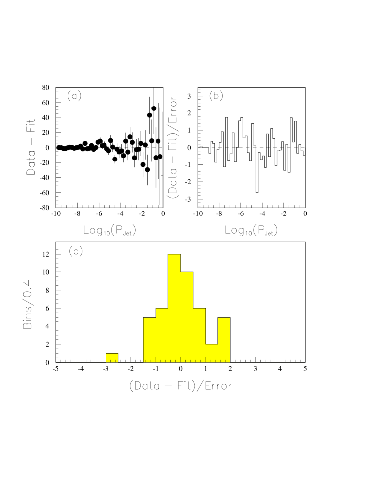
Figure 6: Various comparisons of the data distribution and the fit results. We show (a) the bin by bin difference between the data and the fit results, (b) the bin-by-bin difference scaled to the errors, and (c) the distribution of the difference scaled to the errors, with mean 0.04 and RMS = 0.95. In all cases, the errors are the statistical error in the data points and the fitted results.

For the semi-differential measurements, we do an independent fit of the log${}_{10}(P_{jet})$ distribution and then correct for the acceptance in each ${\rm E}_{\rm T}$ or $\delta\phi$ bin. Table 1 contains a summary of the number of total jets and the number of $\overline{b}$ jets in each ${\rm E}_{\rm T}$ and $\delta\phi$ bin considered.

${\rm E}_{\rm T}$ Range	Number of Jets	Estimated Number
		of $\overline{b}$ Jets
10 — 15	5174	547 $\pm$ 49
15 — 20	3818	618 $\pm$ 47
20 — 25	2563	453 $\pm$ 39
25 — 30	1698	278 $\pm$ 30
30 — 40	1921	327 $\pm$ 33
40 — 50	819	140 $\pm$ 20
50 — 100	849	107 $\pm$ 19
$\delta\phi$ Range
0—$\frac{\pi}{8}$	43	4.8 $+5.5-4.8$
$\frac{\pi}{8}$ — $\frac{\pi}{4}$	83	25.0 $\pm$ 8.6
$\frac{\pi}{4}$ — $\frac{3\pi}{8}$	230	54.7 $\pm$ 13.3
$\frac{3\pi}{8}$ — $\frac{\pi}{2}$	336	78.2 $\pm$ 15.9
$\frac{\pi}{2}$ — $\frac{5\pi}{8}$	519	105. $\pm$ 18.5
$\frac{5\pi}{8}$ — $\frac{3\pi}{4}$	1008	160. $\pm$ 25.
$\frac{3\pi}{4}$ — $\frac{7\pi}{8}$	3229	461. $\pm$ 42.
$\frac{7\pi}{8}$ — $\pi$	11394	1593. $\pm$ 75.

Table 1: $\overline{b}$ fit results as a function of jet ${\rm E}_{\rm T}$ and $\delta\phi$ between the muon and $\overline{b}$ jet. We have not included a common systematic uncertainty of 5.8%.

5 Acceptance and Efficiency

5.1 Muon Requirements

The muon geometric acceptance is the fraction of events with a muon in the good fiducial region of the CMU and CMP chambers, starting from a sample where the muon has $p_{\rm T}>$ 9 GeV/c and $\mid\eta\mid<$ 0.6. Note that this term is only a geometric acceptance and does not include kinematical cuts on the muon.

The geometric acceptance is studied with a $b\rightarrow\mu$ Monte Carlo generator (which includes the sequential decays $b\rightarrow c\mu$), with the input spectra coming from the next to leading order calculation of $b-\overline{b}$ production by Mangano, Nason, and Ridolfi (MNR) [22]. The input spectra use the MRSD0 structure functions [23] and renormalization scale $\mu_{0}=\sqrt{m_{b}^{2}+(p_{\rm T}^{b2}+p_{\rm T}^{\overline{b}2}2)/2}$, with $m_{b}$ = 4.75 GeV/$c^{2}$. This generator produces $b$ quarks and $B$ hadrons, using the Peterson fragmentation form [24] with $\epsilon=0.006~{}\pm~{}0.002$ [25]. $B$ hadrons are decayed according to the CLEO Monte Carlo program, QQ [26]. We select events with a $b\rightarrow\mu$ decay, with muon $p_{\rm T}>$ 9 GeV/c and $\mid\eta\mid<$ 0.6.

For these studies, event vertices are distributed along the $z$ axis as a Gaussian with mean = -1.4 cm and $\sigma$ = 26.65 cm [21], which is a good approximation to the average conditions seen in the data. The muons are propagated to the CMU and CMP chamber radii, including the effects of the central magnetic field and multiple scattering. The acceptance is then defined as the fraction of muons which are in the good fiducial area of both the CMU and CMP chambers and is found to be 53.0 $\pm$ 0.3% (statistical), independent of variations of the $\epsilon$ parameter from 0.004 to 0.008.

The muon trigger and selection depends significantly upon the track reconstruction efficiency in the CTC. We have defined our efficiencies to be multiplicative, so that we can measure them independently. In this section, the efficiencies of the individual selection requirements, and methods of measuring them, are described.

The trigger efficiency is measured using independently triggered samples for each level of the system, where the efficiency is expressed as a function of the muon $p_{\rm T}$. Figure 7 shows the efficiency curves for the 3 levels of the trigger system. The efficiency curves are then convoluted with the $p_{\rm T}$ spectrum of the muons, to extract the efficiency for a muon with $p_{\rm T}>$ 9 GeV/$c$. This convolution is done independently for the differential ${\rm E}_{\rm T}$ cross section bins (see table 2), since the muon $p_{\rm T}$ spectrum may depend upon the transverse momentum distribution of the $\overline{b}$ jet recoiling against the $b\rightarrow\mu$ decay. For $\overline{b}$ jets with ${\rm E}_{\rm T}>$ 10 GeV, the combined L1, L2, and L3 trigger efficiency is measured to be 83.0 $\pm$ 1.7 %.

Figure 7: The trigger efficiency curves for the 3 levels of the trigger system. The trigger efficiency is the product of the three curves, convoluted with the $\mu~{}p_{\rm T}$ spectrum.

The vertex requirement, $\mid z_{0}\mid<30$ cm, is studied in a minimum bias trigger dataset, comparing the vertex distribution to the predicted shape, including the measured longitudinal distribution of the proton and anti-proton bunches and the effects of the accelerator $\beta$ function [21]. The efficiency is found to be 74.2 $\pm$ 2.1 %, where the uncertainty comes from uncertainty in the measured beam longitudinal distributions and $\beta$ function.

The track finding efficiency in the CTC is a function of the density of charged particles. By embedding Monte Carlo simulated track hits into data samples, we quantify the probability of finding the Monte Carlo simulated track as a function of the relative density of CTC hits. The quantified probability is convoluted with the hit density distribution for the muon sample. The track finding efficiency is measured to be 96 $\pm$ 1.7 %, where the uncertainty represents the change in the result using different parametrizations of the probability curve vs hit density.

The combined $\chi^{2}$ matching efficiency is measured in a $J/\psi\rightarrow\mu^{+}\mu^{-}$ sample identified by tracking and mass requirements and is found to be $98.7\pm 0.2$ %. The muon segment reconstruction efficiency is found to $98.1\pm 0.3$ %, resulting in a combined efficiency of $96.8\pm 0.4$ %.

The track finding efficiency in the SVX is studied in the 9 GeV/$c$ muon sample, requiring the CTC track to extrapolate to a good SVX fiducial region. The efficiency is found to be 90 $\pm$ 1%, where the uncertainty is the statistical error only.

${\rm E}_{\rm T}$ bin	Trigger Efficiency
10 — 15 GeV	82.6 $\pm$ 1.7 %
15 — 20 GeV	83.0 $\pm$ 1.7 %
20 — 25 GeV	83.4 $\pm$ 1.7 %
25 — 30 GeV	83.6 $\pm$ 1.7 %
30 — 40 GeV	83.8 $\pm$ 1.7 %
40 — 50 GeV	83.9 $\pm$ 1.7 %
50 — 100 GeV	83.7 $\pm$ 1.7 %
All ${\rm E}_{\rm T}$	83.0 $\pm$ 1.7 %

Table 2: The muon trigger efficiency for each jet ${\rm E}_{\rm T}$ bin. A common 2% uncertainty is assigned to each bin.

Geometric Acceptance	53.0 $\pm$ 0.3 %
CTC Track Finding	96.0 $\pm$ 1.7 %
Matching Efficiency	96.8 $\pm$ 0.4 %
Z Vertex Requirements	74.2 $\pm$ 2.1 %
SVX Track Finding	90 $\pm$ 1 %
Combined Acceptance
and Efficiency	32.9 $\pm$ 1.1 %

Table 3: Summary of muon acceptance and efficiency numbers. The trigger efficiency is applied on a bin by bin basis for the jet ${\rm E}_{\rm T}$ measurement.

5.2 $\overline{b}$ Jet Requirements

The $\overline{b}$ jet acceptance combines the fiducial acceptance of the SVX and the CTC, the track reconstruction efficiency, and fragmentation effects and the $\Delta$R separation requirement. These tracking and $\Delta$R effects are studied separately, with a full simulation used for the combination of the track requirements and fiducial acceptance, while a MNR based $\mu-\overline{b}$ model is used for the $\Delta$R acceptance. The ${\overline{b}}$ jet acceptance is calculated separately as a function of the jet ${\rm E}_{\rm T}$ and azimuthal opening angle between the muon and the jet.

Monte Carlo samples for $b$ and $c$ quarks are produced using ISAJET version 6.43 [27]. The CLEO Monte Carlo program [26] is used to model the decay of $B$ hadrons. $b$ quarks produced using the HERWIG Monte Carlo [28] and PYTHIA Monte Carlo [29] programs are also used for systematic studies. The ISAJET and PYTHIA samples used the Peterson form as the fragmentation model, with $\epsilon=$ 0.006 $\pm$ 0.002. While none of these generators use a NLO calculation of $b$ production, the $\eta$ distribution of the quarks agrees well with the NLO calculation. For tracking efficiency studies, events with a muon with $p_{\rm T}>$ 8 GeV are passed through the full CDF simulation and reconstruction package. The simulation used an average $b$ lifetime of $c\tau$ = 420 $\mu$m [20].

The track acceptance represents the fraction of $\overline{b}$ quarks, ${\rm E}_{\rm T}>$ 10 GeV, $|\eta|<$ 1.5 which produce jets with at least 2 good tracks inside a cone of 0.4 around the jet axis, where there is also a $b$ quark which decays to a muon with $p_{\rm T}>$ 9 GeV within the CMU-CMP acceptance. The average track acceptance for the ${\overline{b}}$ is 51.4 $\pm$ 0.8%. It ranges from 45.7 $\pm$ 1.1% (statistical error only) for 10 $<$ ${\rm E}_{\rm T}$ $<$ 15 GeV to 64.8 $\pm$ 2.6% for 50 $<$ ${\rm E}_{\rm T}$ $<$ 100 GeV.

${\rm E}_{\rm T}$ Range	Track Acceptance	$\Delta$R Acceptance
10 — 15	45.7 $\pm$ 1.1 $\pm$ 2.3 %	86.9 $\pm$ 1.0 ${}^{+1.4}_{-1.6}$ %
15 — 20	55.9 $\pm$ 1.7 $\pm$ 2.8 %	88.2 $\pm$ 1.5 ${}^{+1.7}_{-1.9}$ %
20 — 25	58.1 $\pm$ 2.5 $\pm$ 2.9 %	88.3 $\pm$ 2.0 ${}^{+2.2}_{-2.0}$ %
25 — 30	61.3 $\pm$ 3.5 $\pm$ 3.1 %	88.3 $\pm$ 2.3 ${}^{+3.0}_{-3.5}$ %
30 — 40	61.7 $\pm$ 3.8 $\pm$ 3.1 %	87.9 $\pm$ 3.4 ${}^{+3.6}_{-5.4}$ %
40 — 50	64.8 $\pm$ 2.6 $\pm$ 3.2 %	87.1 $\pm$ 3.5 ${}^{+4.2}_{-5.1}$ %
50 — 100	65.0 $\pm$ 2.6 $\pm$ 3.3 %	85.5 $\pm$ 3.7 ${}^{+5.2}_{-1.9}$ %
$\delta\phi$ Range (radians)
0—$\frac{\pi}{8}$	46.3 $\pm$ 1.4 $\pm$ 2.6 %	6.9 $\pm$ 0.03 ${}^{+0.3}_{-0.2}$ %
$\frac{\pi}{8}$ — $\frac{\pi}{4}$	47.3 $\pm$ 1.4 $\pm$ 2.6 %	20.8 $\pm$ 0.2 ${}^{+2.1}_{-0.3}$ %
$\frac{\pi}{4}$ — $\frac{3\pi}{8}$	51.4 $\pm$ 0.8 $\pm$ 2.6 %	74.7 $\pm$ 0.9 ${}^{+6.0}_{-0.0}$ %
$\frac{3\pi}{8}$ — $\pi$	51.4 $\pm$ 0.8 $\pm$ 2.6 %	100 %

Table 4: $\mu-\overline{b}$ track and $\Delta$R acceptance as a function of jet ${\rm E}_{\rm T}$ and $\delta\phi$ (statistical and systematic uncertainties). There is a common (relative) systematic uncertainty of 5% in the tracking efficiency. For $\delta\phi>$ 1 radian, the $\Delta$R acceptance is 100% by definition.

We have compared the values for the ${\overline{b}}$ track acceptance from ISAJET samples to the acceptance from HERWIG samples. The acceptance agrees within the statistical error in the samples as a function of ${\rm E}_{\rm T}$, differing at the 5% level. We include this variation as an additional systematic uncertainty on the track acceptance. Comparisons of inclusive jet track acceptances from an ISAJET sample and from data show reasonable agreement.

For the calculation of the $\Delta$R acceptance, we have used a model based on the MNR calculation [22]. This calculation can be used to give exact ${\cal O}(\alpha_{s}^{3})$ results in situations where kinematical cuts have been applied at the parton level. We have made additions to the calculation to model the $\mu-\overline{b}$ differential cross sections.

The MNR calculation [22] produces the vectors $p^{b}$, $p^{\overline{b}}$, and $p^{gluon}$ with appropriate weights. We include additional weighting for the following:

• Probability of $p_{\rm T}^{\mu}>$ 9 GeV/c for given $p_{\rm T}^{b}$, ${\cal P}(p_{\rm T}^{\mu},p_{\rm T}^{b})$

• Probability of ${\rm E}_{\rm T}^{\overline{b}}$ jet in a given ${\rm E}_{\rm T}$ bin for given $p_{\rm T}^{\overline{b}}$, ${\cal P}({\rm E}_{\rm T}^{\overline{b}},p_{\rm T}^{\overline{b}})$

${\cal P}(p_{\rm T}^{\mu},p_{\rm T}^{b})$ is defined as the fraction of $b$ quarks, with given $p_{\rm T}^{b}$, which decay into muons with $p_{\rm T}^{\mu}>$ 9 GeV/c. We use the $b\rightarrow\mu$ Monte Carlo generator described above to derive this function, using B$(b\rightarrow\mu)$ = 0.103 $\pm$ 0.005 [8]. Since the probability is defined as a function of $p_{\rm T}^{b}$, the exact shape of the $p_{\rm T}^{b}$ distribution does not enter into the result. Figure 8 shows the value ${\cal P}(p_{\rm T}^{\mu},p_{\rm T}^{b})$ as a function of $p_{\rm T}^{b}$. The three curves are for different values of the Peterson $\epsilon$ parameter used in the fragmentation model. In addition to this probability weighting, we also smear the $b$ quark direction in pseudo-rapidity and azimuth. The smearing is based on the results from the $b\rightarrow\mu$ Monte Carlo generator.

Figure 8: The probability of a $b\rightarrow\mu$ decay, with $p_{\rm T}^{\mu}>$ 9 GeV/c, as a function of $p_{\rm T}^{b}$. We have included the branching fraction $B(b\rightarrow\mu)=0.103$. The curves represent three choices of the Peterson $\epsilon$ parameter used in the fragmentation process.

${\cal P}({\rm E}_{\rm T}^{\overline{b}},p_{\rm T}^{\overline{b}})$ is defined as the probability that a $\overline{b}$ quark, with given $p_{\rm T}^{\overline{b}}$, would produce a jet with given ${\rm E}_{\rm T}^{\overline{b}}$. Using the methods outlined in section 6, we have a binned probability distribution in ${\rm E}_{\rm T}$ for each $p_{\rm T}^{\overline{b}}$. Since the measured jet ${\rm E}_{\rm T}$ integrates over a range in pseudo-rapidity and azimuth (a cone of radius 0.4), we approximate this clustering effect by clustering partons (adding the $\overline{b}$ and the gluon momenta vectorially) within the same cone size. For the rest of this paper, when we discuss the ${\rm E}_{\rm T}^{\overline{b}}$ or $p_{\rm T}^{\overline{b}}$ theory distributions, it means the clustered partons ${\rm E}_{\rm T}$ or $p_{\rm T}$.

We use a renormalization and factorization scale $\mu_{0}=\sqrt{m_{b}^{2}+(p_{\rm T}^{b2}+p_{\rm T}^{\overline{b}2})/2}$, MRSA structure functions [30], and $m_{b}$ = 4.75 GeV/$c^{2}$. Applying the additional weights and the appropriate kinematical cuts ($\mid\eta^{\mu}\mid<$ 0.6 and $\mid\eta^{\overline{b}}\mid<$ 1.5), we obtain the calculated d$\sigma$/d${\rm E}_{\rm T}^{\overline{b}}$ and d$\sigma$/d$\delta\phi(\mu-\overline{b})$ distributions. We create the same distributions with the requirement that the muon and $\overline{b}$ be separated by $\Delta$R $>$ 1 and do a bin by bin comparison of the calculated cross sections to define the $\Delta$R acceptance. We have varied the renormalization scale, $b$ quark mass, and parton distribution functions used in the MNR calculation to estimate the systematic uncertainties in the $\Delta$R acceptance. Table 4 shows the bin by bin values used in the differential cross section measurements.

6 Cross Section Results

The cross section results are presented as $\mu-\overline{b}$ cross sections. Since we have not specifically done flavor identification, there is an additional factor of $1/2$ in the calculation of the cross sections. For the semi-differential measurements, we do an independent fit of the log${}_{10}(P_{jet})$ distribution and then correct for the acceptance in each ${\rm E}_{\rm T}$ or $\delta\phi$ bin. With the number of $\overline{b}$ jets from table 1, the bin by bin trigger efficiencies from table 2, the combined muon acceptance and efficiency from table 3, and the $\overline{b}$ track and $\Delta$R acceptances from table 4, we calculate the the cross section in each ${\rm E}_{\rm T}$ and $\delta\phi$ bin considered. The sum of the 7 ${\rm E}_{\rm T}$ bins is 614.4 $\pm$ 63.0 pb and the sum of the 8 $\delta\phi$ bins is 633.0 $\pm$ 70.6 pb. The results are summarized in table 5.

${\rm E}_{\rm T}$ Range	Cross Section (pb)
10 — 15	168.1${}^{+15.8}_{-15.8}$
15 — 20	152.2${}^{+12.7}_{-12.8}$
20 — 25	106.6${}^{+10.5}_{-10.5}$
25 — 30	61.93${}^{+7.79}_{-7.79}$
30 — 40	72.53${}^{+8.96}_{-9.43}$
40 — 50	29.81${}^{+4.60}_{-4.68}$
50 — 100	23.13${}^{+4.38}_{-4.23}$
$\delta\phi$ Range
0—$\frac{\pi}{8}$	18.36${}^{+24.38}_{-18.36}$
$\frac{\pi}{8}$ — $\frac{\pi}{4}$	30.86${}^{+18.63}_{-10.91}$
$\frac{\pi}{4}$ — $\frac{3\pi}{8}$	17.30${}^{+4.60}_{-4.21}$
$\frac{3\pi}{8}$ — $\frac{\pi}{2}$	18.48 $\pm$ 3.76
$\frac{\pi}{2}$ — $\frac{5\pi}{8}$	24.81 $\pm$ 4.37
$\frac{5\pi}{8}$ — $\frac{3\pi}{4}$	37.81 $\pm$ 5.91
$\frac{3\pi}{4}$ — $\frac{7\pi}{8}$	108.9 $\pm$ 9.93
$\frac{7\pi}{8}$ — $\pi$	376.4 $\pm$ 17.7

Table 5: $\mu-\overline{b}$ cross sections as a function of jet ${\rm E}_{\rm T}$ and $\delta\phi$ between the muon and $\overline{b}$ jet. We have not included a common systematic uncertainty of 9.3% in the results. Physics backgrounds have not been subtracted at this stage.

6.1 Physics Backgrounds

There are backgrounds which need to be included before comparing to theoretical predictions on $b-\overline{b}$ production, since there are additional sources of $\mu-\overline{b}$ production. Specifically, the decay products of light mesons ($\pi$, $K$) produced in association with $b-\overline{b}$ pairs or heavy particles (e.g, the $Z^{\circ}$ boson, top quark production) can give a similar signature.

A contribution to the sample occurs when the identified muon is not coming from a $b$ quark decay but instead from the decay of a light meson ($\pi$ or $K$) or charm quark. In the inclusive muon sample, the $b$ fraction is measured to be approximately 40% [15], with a charm fraction of approximately 20% and the remaining 40% from the decay of light mesons. Since jets from gluons are the dominant production process in this jet ${\rm E}_{\rm T}$ range, we assume that the light mesons come predominantly from gluon jets. With the further assumption that the gluon splitting to $b\overline{b}$ probability is approximately 1.5% [33], we estimate that in 0.6% ($0.015\times 0.4$) of the muon events we correctly identify the $\overline{b}$ but the muon is from a light meson decay. The case where the identified muon comes from the decay of a charm particle can be estimated in a similar manner. With the same assumptions about the gluon splitting to heavy quark probability (1.5%), a measured charm fraction of 20%, and that approximately 75% of charm quarks are produced via gluon splitting, we estimate that in 0.2% ($0.015\times 0.75\times 0.2$) of the muon events we correctly identify the $\overline{b}$ but the muon is from a charm particle decay.

With an identified fraction of 40% $b$ muons and 50% of the produced $b$’s from gluon splitting [33], in 20% of the muon events we correctly identify the $\overline{b}$ and the muon from the $b$ decay. Combining these calculations yields a fractional background in the $\mu-\overline{b}$ cross section of 0.04 ($=(0.006+0.002)/0.20$). We assume that this background has the same shape as the signal and reduce the cross sections by a constant 4.0 $\pm$ 2.0% (the uncertainty is taken as half the change).

We have used the PYTHIA Monte Carlo program to generate $Z^{\circ}\rightarrow b\overline{b}$ events, and the CLEO Monte Carlo program for the decay of the resulting $B$ hadrons. We normalize the production cross section to measured CDF cross section of $Z^{\circ}\rightarrow e^{+}e^{-}$ [8, 31], and apply the same $\mu$ and $\overline{b}$ jet requirements as presented in section 3. The predicted cross section remaining after these requirements is 3.6 $\pm$ 0.28 pb, where the uncertainty includes the relative normalization to the dielectron decay mode, the $b\rightarrow\mu$ branching fraction, and acceptance uncertainties. Table 6 shows the contributions from this process in the same ${\rm E}_{\rm T}$ and $\delta\phi$ bins as in table 5.

${\rm E}_{\rm T}$ Range	Cross Section (pb)
	Statistical Uncertainty only
10 — 15	0.43 $\pm$ 0.06
15 — 20	0.75 $\pm$ 0.08
20 — 25	0.82 $\pm$ 0.09
25 — 30	0.60 $\pm$ 0.07
30 — 40	0.87 $\pm$ 0.10
40 — 50	0.12 $\pm$ 0.02
50 — 100	0.015 $\pm$ 0.008
$\delta\phi$ Range
0—$\frac{\pi}{8}$	0
$\frac{\pi}{8}$ — $\frac{\pi}{4}$	0
$\frac{\pi}{4}$ — $\frac{3\pi}{8}$	0.015 $\pm$ 0.014
$\frac{3\pi}{8}$ — $\frac{\pi}{2}$	0.031 $\pm$ 0.012
$\frac{\pi}{2}$ — $\frac{5\pi}{8}$	0.036 $\pm$ 0.013
$\frac{5\pi}{8}$ — $\frac{3\pi}{4}$	0.11 $\pm$ 0.024
$\frac{3\pi}{4}$ — $\frac{7\pi}{8}$	0.53 $\pm$ 0.05
$\frac{7\pi}{8}$ — $\pi$	2.88 $\pm$ 0.12

Table 6: Contributions from $Z^{\circ}\rightarrow\mu\overline{b}$ to the cross section as a function jet ${\rm E}_{\rm T}$ and $\delta\phi$ between the $\mu$ and $\overline{b}$ jet. There is an addition 8.0% uncertainty in the overall normalization.

Top quark production and decay can also contribute to the $\mu-\overline{b}$ cross sections. The CDF measurement of the total top cross section is $6.8^{+3.6}_{-2.4}$ pb [32]. However, once we account for branching fractions and acceptance criteria, the total cross section from this process is less than 1 pb and will not be considered further.

6.2 Jet Unsmearing Procedure

The cross sections measured above depend upon the selection of jets with ${\rm E}_{\rm T}>$ 10 GeV, and in the case of the d$\sigma$/d${\rm E}_{\rm T}$ distribution, depend upon the binning of the distribution. Jets coming from $\overline{b}$ quarks with transverse momentum $p_{\rm T}^{\overline{b}}$ will contribute to more than one bin in the measured distribution, due to the combined effects of calorimeter energy response, calorimeter energy resolution, and quark fragmentation. An unsmearing procedure has been developed at CDF to account for these effects.

We use Monte Carlo produced samples to define the expected jet ${\rm E}_{\rm T}$ response distribution for a given quark $p_{\rm T}$. An iterative procedure is used to correct the measured cross sections. The quark $p_{\rm T}$ distribution is described by a smooth function and smeared with the simulation derived ${\rm E}_{\rm T}$ response functions. The input distribution is adjusted until the smeared distribution matches the measured distribution. We then perform a simultaneous unfolding of the measured jet ${\rm E}_{\rm T}$ spectrum to the parton $p_{\rm T}$ spectrum to account for energy loss and resolution. This unfolding corrects both the cross section and ${\rm E}_{\rm T}$ ($p_{\rm T}$) axes.

6.2.1 Response Functions

The calorimeter single particle response in the range 0.5 to 227 GeV has been determined from both test beam data and isolated tracks from collider data. A Monte Carlo simulation incorporating the calorimeter response and the ISAJET, HERWIG, and PYTHIA samples is used to determine a response function for $\overline{b}$ jets in the ${\rm E}_{\rm T}$ range 5 to 150 GeV, including energy loss, resolution, and jet finding efficiency effects. For each $p_{\rm T}$, the response function represents the probability distribution for measuring a particular value of ${\rm E}_{\rm T}$. These response functions are convoluted with the expected $\overline{b}~{}p_{\rm T}$ distributions, creating an expected ${\rm E}_{\rm T}$ distribution.

6.2.2 Unsmearing

The input $\overline{b}$ distribution comes from the $\mu-\overline{b}$ model described in section 5, where we have required a muon with $p_{\rm T}>$ 9 GeV/c. We have parametrized the distribution with a multi-quadric function and varied a scale parameter until the smeared distribution matches the measured distribution. Figure 9 shows the best match $\overline{b}$ $p_{\rm T}$ distribution, overlayed with the smeared distribution. Table 7 shows the unfolding effects on the cross section and transverse momentum. Note that the unsmearing procedure introduces correlated systematic uncertainties in the bins.

Figure 9: The best match $p_{\rm T}^{\overline{b}}$ distribution, overlayed with the smeared distribution (dashed) and the data ${\rm E}_{\rm T}$ measurement. The process is reversed to take the data ${\rm E}_{\rm T}$ distribution to a $p_{\rm T}$ distribution.

Jet ${\rm E}_{\rm T}$ Bin	Mean Jet ${\rm E}_{\rm T}$	$\sigma$ (pb/GeV)	Mean ${\overline{b}}~{}p_{\rm T}$	$\sigma$ (pb/GeV/c)
10 — 15	12.38	32.20	25.28	27.66
15 — 20	17.35	29.07	30.67	24.62
20 — 25	22.30	20.30	35.99	18.78
25 — 30	27.34	11.77	41.20	12.52
30 — 40	34.31	6.88	48.38	7.13
40 — 50	44.36	2.85	59.00	3.05
50 — 100	63.19	0.44	79.18	0.57

Table 7: Smeared and unsmeared means and cross sections for the 7 bins in the differential $p_{\rm T}$ measurement. The cross sections are after background subraction and are presented here without uncertainties. Note that the unsmearing procedure introduces correlated uncertainties in the bins.

6.2.3 Systematic Uncertainties

Systematic uncertainties in the smearing procedure arise from uncertainties in the knowledge of the calorimeter energy scale, the calorimeter resolution, the jet finding efficiency, the $\overline{b}$ quark fragmentation, and the effects of the underlying event in defining the jet energy. The parameters in the smearing procedure are adjusted to account for these uncertainties, the input distribution is smeared, and the difference between the standard smeared distribution and the new smeared distribution is used to estimate the bin by bin systematic uncertainties. The uncertainties are added in quadrature to extract a total systematic uncertainty. Table 8 contains the bin by bin systematic uncertainties.

Variation	10 — 15 GeV ${\rm E}_{\rm T}$	15 — 20 GeV ${\rm E}_{\rm T}$	20 — 25 GeV ${\rm E}_{\rm T}$
Energy Scale	+ 7.2% - 4.6%	+ 4.7% - 3.5%	+ 9.1% - 7.3%
Underlying event	+ 0.2% - 0.2%	+ 0.1% - 0.2%	+ 0.2% - 0.2%
Calorimeter Resolution	+ 4.4% - 4.2%	+ 2.6% - 2.5%	+ 4.1% - 4.1%
Jet Finding	$\pm$ 2.6%	$\pm$ 0.7%	$\pm$ 1.0%
$b$ Fragmentation	+ 1.0%	- 4.0%	- 4.7%
Total	+ 8.9% - 6.7%	+ 5.4% - 5.9%	+10.0% - 9.6%
	25 — 30 GeV ${\rm E}_{\rm T}$	30 — 40 GeV ${\rm E}_{\rm T}$	40 — 50 GeV ${\rm E}_{\rm T}$
Energy Scale	+12.5% -10.2%	+16.5% -13.4%	+20.7% -16.5%
Underlying event	+ 0.3% - 0.3%	+ 0.4% - 0.4%	+ 0.4% - 0.4%
Calorimeter Resolution	+ 3.5% - 3.5%	+ 0.9% - 0.9%	+ 4.5% - 4.5%
Jet Finding	$\pm$ 0.3%	$\pm$ 0.0%	$\pm$ 0.0%
$b$ Fragmentation	- 4.4%	- 3.4%	+ 1.6%
Total	+13.0% -11.6%	+16.5% -13.9%	+21.2% -17.2%
	50 — 100 GeV ${\rm E}_{\rm T}$
Energy Scale	+27.8% -21.3%
Underlying event	+ 0.4% - 0.4%
Calorimeter Resolution	+12.7% -12.7%
Jet Finding	$\pm$ 0.0%
$b$ Fragmentation	+ 1.0%
Total	+30.6% -24.8%

Table 8: Systematic uncertainties for each bin in the $\mu-{\overline{b}}$ differential jet ${\rm E}_{\rm T}$ distribution. There are bin to bin correlations for each systematic variation.

6.2.4 $\overline{b}$ Jet $p_{\rm T}^{min}$ Definition

For future comparisons to theoretical predictions on overall normalization, we need to define a $p_{\rm T}^{min}$ threshold for the recoiling $\overline{b}$ quark. The standard definition is to take the $p_{\rm T}$ value where $>$90% of all decays pass the kinematic cuts. In this case, we need to find the point where $>$ 90% of all jets have E${}_{T}>$ 10 GeV. We begin with the $\overline{b}$ $p_{\rm T}$ spectrum shown in figure 9 and apply the resolution smearing to this distribution. We weight each bin in the $p_{\rm T}$ spectrum by the probability that a $\overline{b}$ quark with that $p_{\rm T}$ would give a jet with E${}_{T}>$ 10 GeV. Integrating the resulting weighted distribution gives a 90% $p_{\rm T}^{min}$ value of 20.7 GeV/c for the $\overline{b}$ jet.

Figure 10: The differential ${\rm E}_{\rm T}$ cross section, for $p_{\rm T}^{\mu}>~{}9$ GeV/c, $|\eta^{\mu}|<$ 0.6, ${\rm E}_{\rm T}^{\overline{b}}>$ 10 GeV, $|\eta^{\overline{b}}|<$ 1.5, compared to theoretical predictions. The data points have a common systematic of $\pm$ 9.5%. The common uncertainty in the theory points comes from the muonic branching fraction and fragmentation model. The theory points do include uncertainties from the smearing procedure.

6.3 Comparison with NLO QCD

In figure 10, we show a comparison of the differential jet ${\rm E}_{\rm T}$ cross section,

$$\frac{{\rm d}\sigma}{{\rm dE}_{\rm T}^{\overline{b}}}(p_{\rm T}^{\mu}>9~{}{\rm GeV/c},|\eta^{b}|<1,|\eta^{\overline{b}}|<1.5,{\rm E}_{\rm T}^{\overline{b}}>10~{}{\rm GeV})$$

to a prediction from the $\mu-\overline{b}$ model discussed in section 3. There is a 9.5% common uncertainty in the measured points, coming from the jet probability fit (5.8%), the $\overline{b}$ jet tracking efficiency (5%), the muon acceptance and identification efficiencies (3.9%), the luminosity normalization (3.6%), and the remaining background subtraction (2%). This common uncertainty is displayed separately. The uncertainty in the model prediction represents the uncertainty from the muonic branching fraction (5%) [8], the acceptance of the muon $p_{\rm T}$ cut from variations in the fragmentation model (5%), which are common to all points, and the uncertainties associated with $p_{\rm T}$ to ${\rm E}_{\rm T}$ smearing. The data has an integral value of 586. $\pm$ 61.8 pb, while the model predicts an integral value of 383.5 $\pm$ 5.9 pb.

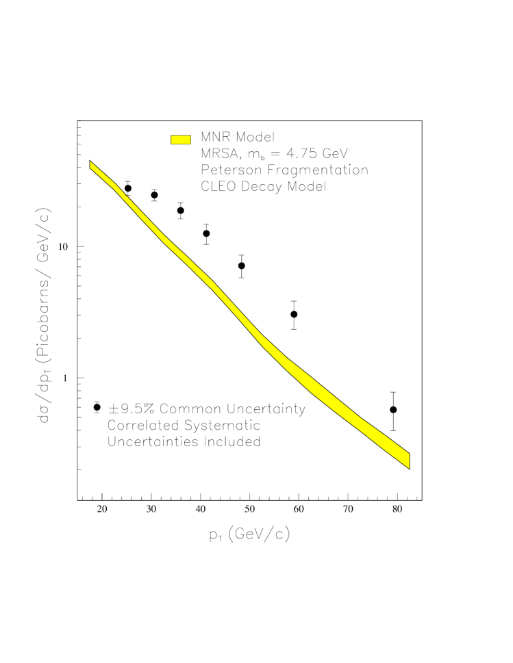
Figure 11: The differential $p_{t}$ cross section, for $p_{\rm T}^{\mu}>~{}9$ GeV/c, $|\eta^{\mu}|<$ 0.6, $|\eta^{\overline{b}}|<$ 1.5, compared to theoretical predictions. The data points have a common systematic of $\pm$ 9.5% and there are correlated systematic uncertainties. The uncertainty in the theory curves comes from the muonic branching fraction and fragmentation model.

In figure 11, we show the unsmeared differential jet $p_{\rm T}$ cross section,

$$\frac{{\rm d}\sigma}{{\rm d}p_{\rm T}^{\overline{b}}}(p_{\rm T}^{\mu}>9~{}{\rm GeV/c},|\eta^{\mu}|<0.6,|\eta^{\overline{b}}|<1.5)$$

compared to the $\overline{b}~{}p_{\rm T}$ prediction from the $\mu-\overline{b}$ model, where we have included systematic uncertainties associated with the resolution smearing on the measured points. Again, the common normalization uncertainties are displayed separately.

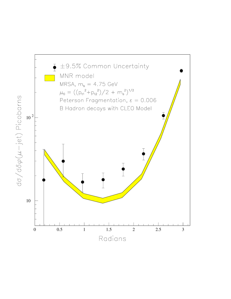
Figure 12: The differential $\delta\phi$ cross sections, for $p_{\rm T}^{\mu}>~{}9$ GeV/c, $|\eta^{\mu}|<$ 0.6, ${\rm E}_{\rm T}^{\overline{b}}>$ 10 GeV, $|\eta^{\overline{b}}|<$ 1.5 compared to theoretical predictions. The data points have a common systematic of $\pm$ 9.5%. The uncertainty in the theory curves comes from the muonic branching fraction and fragmentation model.

In figure 12, we show a comparison of the differential $\delta\phi(\mu-\overline{b})$ cross section,

$$\frac{{\rm d}\sigma}{{\rm d}\delta\phi^{\mu-\overline{b}}}(p_{\rm T}^{\mu}>9~{}{\rm GeV/c},|\eta^{\mu}|<0.6,{\rm E}_{\rm T}^{\overline{b}}>10~{}{\rm GeV},|\eta^{\overline{b}}|<1.5)$$

to the predictions from the $\mu-\overline{b}$ model. The uncertainty in the theoretical prediction represents the uncertainty in the muonic branching fraction and fragmentation model only.

While we find qualitative agreement in shape between the measured distributions and model predictions, there are some differences. To investigate in more detail, we present in figure 13 the experimental results minus the model prediction, scaled to the model prediction for the ${\rm E}_{\rm T}$, $p_{\rm T}$, and $\delta\phi$ distributions. The ${\rm E}_{\rm T}(p_{\rm T}$) distributions have similar shapes for ${\rm E}_{\rm T}(p_{\rm T})>$ 20 GeV( 35 GeV/c), but different normalizations. At lower values of ${\rm E}_{\rm T}$ ($p_{\rm T}$), the measurements and predictions are in agreement. The data $\delta\phi$ distribution is somewhat broader than the model predictions, with enhancement in the region $\pi/4$ to $3\pi/4$, as well as being at consistently higher values. We have also shown how the model prediction changes with change of the renormalization and factorization scale, by plotting the prediction for scale $\mu_{0}/2$ minus the prediction for $\mu_{0}$, scaled to the prediction for $\mu_{0}$. The integral cross section increases by 7%, with very little change as a function of ${\rm E}_{\rm T}$ or $p_{\rm T}$. In the $\delta\phi$ distribution, the $\mu_{0}/2$ prediction is uniformly larger than the $\mu_{0}$ prediction, except for the region $\delta\phi\approx\pi$.

Figure 13: For the (a) d$\sigma$/d${\rm E}_{\rm T}$, (b) d$\sigma$/d$p_{\rm T}$, and (c) d$\sigma$/d$\delta\phi$ distributions, we plot the difference between the data measurement (filled circles) and the model prediction, scaled to the model prediction. There is a common systematic uncertainty of 9.5% in all the points, which has not been included in the error bar. The open circles are the model prediction for renormalization scale of $\mu_{0}/2$ minus the model prediction for $\mu_{0}$, scaled to the model prediction for $\mu_{0}$.

Recent work has shown that the addition of an intrinsic $k_{\rm T}$ kick to a next-to-leading order QCD calculation improves the agreement between measurements and predictions for both direct photon production [34] and charm production [3]. We have investigated the effects of additional intrinsic $k_{\rm T}$ in the $\mu-\overline{b}$ model. We use a Gaussian distribution with mean 0 and adjustable width to model the magnitude of the kick, with a random azimuthal direction. With widths of 2 - 4 GeV/c, we find that the dominant effects occur for $\delta\phi<$ 1 radian. The cross section for $\delta\phi<$ 1 is predicted to change by approximately 7% with a width of 4 GeV/c. With the current statistical uncertainties at small $\delta\phi$ (ranging from 25 - 100 %), we are unable to distinguish effects at that level. Similarly, the dominant effect in the $p_{\rm T}^{\overline{b}}$ distribution occurs in regions where we have no sensitivity ($p_{\rm T}^{\overline{b}}<$ 20 GeV/c). We conclude that the addition of intrinsic $k_{\rm T}$ with width of 4 GeV/c does not account for the difference between the model prediction and the measurement.

7 Conclusions

We have presented results on the semi-differential $\mu-\overline{b}$ cross sections as a function of the $\overline{b}$ jet transverse energy (d$\sigma$/d${\rm E}_{\rm T}$), $\overline{b}$ transverse momentum (d$\sigma$/d$p_{\rm T}$), and the azimuthal opening angle between the muon and the $\overline{b}$ jet (d$\sigma$/d$\delta\phi$). These results are based on precision track reconstruction in jets. The effects of detector response and resolution have been unfolded to translate the results from $\overline{b}$ jets to $\overline{b}$ quarks. We have compared these results to a model based on a full NLO QCD calculation [22]. We have investigated the effects an additional intrinsic $k_{\rm T}$ and find that it cannot account for the difference between the measurements and the model prediction. Unlike previous CDF measurements [1, 4], a normalization change alone does not account for the differences between this measurement and the model prediction.

We thank the Fermilab staff and the technical staffs of the participating institutions for their vital contributions. This work was supported by the U.S. Department of Energy and National Science Foundation; the Italian Istituto Nazionale di Fisica Nucleare; the Ministry of Education, Science and Culture of Japan; the Natural Sciences and Engineering Research Council of Canada; the National Science Council of the Republic of China; the A. P. Sloan Foundation; and the Alexander von Humboldt-Stiftung.

References

- [1] F. Abe, et al., Phys. Rev. Lett., 71, 2396 (1993).
- [2] S. Abachi, et al., Phys. Rev. Lett., 74, 3548 (1995).
- [3] S. Frixione, et al., Nucl. Phys. B 431, 453 (1994).
- [4] F. Abe, et al., FERMILAB-PUB-95/48-E, submitted to Phys. Rev. Lett.
- [5] F. DeJongh, in the Proceedings of the Workshop on B Physics at Hadron Colliders, ed. by P. McBride and C.S. Mishra, Snowmass, Co., June 1993.
- [6] The CDF coordinate system defines along the proton-beam direction, as the polar angle, and as the azimuthal angle. The pseudorapidity, , is defined as .
- [7] F. Abe, et al., Fermilab-PUB-94/131-E.
- [8] L. Montanet, et al., Particle Data Group, Phys. Rev. D50, 1173 (1994).
-
[9]
F. Abe, et al., Phys. Rev. D45, 1448 (1992);
F. Abe, et al., Phys. Rev. D47, 4857 (1993). - [10] F. Abe, et al., Nucl. Instr. Meth. A271, 387 (1988) and references therein.
- [11] D. Amidei, et al., Nucl. Instr. Meth. A350, 73 (1994).
- [12] F. Bedeschi, et al., Nucl. Instr. Meth. A268, 51 (1988).
- [13] G. Ascoli, et al., Nucl. Instr. Meth. A268, 33 (1988).
- [14] J. Chapman, et al., to be submitted to Nucl. Instr. Meth..
- [15] F. Abe, et al., Phys. Rev. D50 2966 (1994).
- [16] D. Amidei, et al., Nucl. Instr. Meth. A269, 51 (1988).
- [17] G. W. Foster, et al., Nucl. Instr. Meth. A269, 93 (1988).
- [18] D. Buskulic, et al., Phys. Lett. B 313, 535 (1993).
- [19] F. Abe, et al., Phys. Rev. Lett. 71, 3421 (1993), CDF presents an error of 5.8%.
- [20] In the fall of 1993, the world average hadron lifetime was 1.4 psec, from LEP and TeVatron experiments (see R. van Kooten, in Results and Perspectives in Particle Physics, Proceedings of the 7th Rencontres de Physique de la Vallee d’Aoste, La Thuile, Italy, 1993, ed. by M. Greco (Editions Frontieres, Gif-sur-Yvette)). Uncertainty in this quantity is included as a systematic in the fitting procedure.
- [21] W. Badgett, Ph.D. thesis, University of Michigan, 1994 (unpublished).
- [22] M. Mangano, P. Nason, and G. Ridolfi, Nucl. Phys. B373, 295 (1992). The FORTRAN code is available from the authors.
- [23] A.D. Martin, R.G. Roberts, and W.J. Stirling, RAL-92-021 (1992).
- [24] C. Peterson, et al., Phys. Rev. D 27, 105 (1983).
- [25] J. Chrin, Z. Phys. C 36, 165 (1987).
- [26] P. Avery, K. Read, and G. Trahern, Cornell Internal Note CSN-212, March 25, 1985 (unpublished).
- [27] F. Paige and S.D. Protopopescu, BNL Report No. 38034, 1986 (unpublished). We used version 6.36.
-
[28]
G. Marchesini and B.R. Webber, Nucl. Phys. B310, (1988), 461;
G. Marchesini, et al., Comput. Phys. Comm. 67 465 (1992). - [29] H. Bengtsson and T. Sjstrand, Comput. Phys. Commun. 46, 43 (1987).
- [30] A.D. Martin, W.J. Stirling, and R.G. Roberts, RAL-94-055, DTP/94/34 (1994).
- [31] F. Abe, et al., Phys. Rev. D44, 29 (1991).
- [32] F. Abe, et al., Phys. Rev. Lett. 74, 2626 (1995).
- [33] These estimates are derived using the next-to-leading order calculations from reference [22]; M. Seymour, Z. Phys. C 63 99 (1995).
- [34] J. Huston, et al., Phys. Rev. D51, 6139 (1995).