Search for Exclusive Charmless Hadronic B Decays

Abstract

We have searched for two-body charmless hadronic decays of $B$ mesons. Final states include $\pi\pi$, $K\pi$, and $KK$ with both charged and neutral kaons and pions; $\pi\rho$, $K\rho$, and $K^{*}\pi$; and $K\phi$, $K^{*}\phi$, and $\phi\phi$. The data used in this analysis consist of 2.6 million $B\bar{B}$ pairs produced at the $\Upsilon(4S)$ taken with the CLEO-II detector at the Cornell Electron Storage Ring (CESR). We measure the branching fraction of the sum of $B^{0}\rightarrow\pi^{+}\pi^{-}$ and $B^{0}\rightarrow K^{+}\pi^{-}$ to be $(1.8^{+0.6+0.2}_{-0.5-0.3}\pm 0.2)\times 10^{-5}$. In addition, we place upper limits on individual branching fractions in the range from $10^{-4}$ to $10^{-6}$.

I Introduction

The decays of $B$ mesons to two charmless hadrons can be described by a $b\rightarrow u$ tree-level spectator diagram (Figure 1a), or a $b\rightarrow sg$ one-loop “penguin-diagram” (Figure 1b) and to a lesser extent, by the color-suppressed tree (Figure 1c) or CKM-suppressed $b\rightarrow dg$ penguin diagrams. Although such decays can also include contributions from $b\rightarrow u$ $W$-exchange (Figure 1d), annihilation (Figure 1e), or vertical $W$ loop (Figure 1f) processes, these contributions are expected to be negligible in most cases.

Decays such as $B^{0}\rightarrow\pi^{+}\pi^{-}$ and $B^{0}\rightarrow\pi^{\pm}\rho^{\mp}$ are expected to be dominated by the $b\rightarrow u$ spectator transition, and measurements of their branching fractions could be used to extract a value for $|V_{ub}|$. The decay mode $B^{0}\rightarrow\pi^{+}\pi^{-}$ can be used to measure $CP$ violation in the $B$ sector at both asymmetric $B$ factories [1] and hadron colliders[2]. Since the $\pi^{+}\pi^{-}$ final state is a $CP$ eigenstate, $CP$ violation can arise from interference between the amplitude for direct decay and the amplitude for the process in which the $B^{0}$ first mixes into a $\bar{B}^{0}$ and then decays. Measurement of the time evolution of the rate asymmetry leads to a measurement of $\sin 2\alpha$, where $\alpha$ is one of the angles in the unitarity triangle[3]. If the $B^{0}\rightarrow\pi^{+}\pi^{-}$ decay has a non-negligible contribution from the $b\rightarrow dg$ penguin, interference between the spectator and penguin contributions will contaminate the measurement of $CP$ violation via mixing [4], an effect known as “penguin pollution.” If this is the case, the penguin and spectator effects can be disentangled by also measuring the isospin-related decays $B^{0}\rightarrow\pi^{0}\pi^{0}$ and $B^{\pm}\rightarrow\pi^{\pm}\pi^{0}$ [5]. Alternatively, SU(3) symmetry can be used to relate $B^{0}\rightarrow\pi^{+}\pi^{-}$ and $B^{0}\rightarrow K^{+}\pi^{-}$ [6, 7]. Penguin and spectator effects may then be disentangled [6] once the ratio of the two branching fractions and $\sin 2\beta$[3] are measured.

Decays such as $B^{0}\rightarrow K^{+}\pi^{-}$ and $B^{0}\rightarrow K^{*+}\pi^{-}$ are expected to be dominated by the $b\rightarrow sg$ penguin process, with a small contribution from a Cabibbo-suppressed $b\rightarrow u$ spectator process. Interference between the penguin and spectator amplitudes can give rise to direct $CP$ violation, which will manifest itself as a rate asymmetry for decays of $B^{0}$ and $\bar{B}^{0}$ mesons, but the presence of hadronic phases complicates the extraction of the $CP$ violation parameters.

There has been discussion in recent literature about extracting the unitarity angles using precise time-integrated measurements of $B$ decay rates. Gronau, Rosner, and London have proposed [8] using isospin relations and flavor SU(3) symmetry to extract, for example, the unitarity angle $\gamma$ by measuring the rates of $B^{+}$ decays to $K^{0}\pi^{+}$, $K^{+}\pi^{0}$, and $\pi^{+}\pi^{0}$ and their charge conjugates. More recent publications [9, 10, 11, 12] have questioned whether electroweak penguin contributions ($b\rightarrow s\gamma$, $b\rightarrow sZ$) are large enough to invalidate isospin relationships and whether SU(3) symmetry-breaking effects can be taken into account. If it is possible to extract unitarity angles from rate measurements alone, the measurements could be made at either symmetric or asymmetric $B$ factories (CESR, KEK, SLAC), but will require excellent particle identification to distinguish between the $K\pi$ and $\pi\pi$ modes.

Decays such as $B\rightarrow K\phi$ and $B^{+}\rightarrow K^{0}\pi^{+}$ cannot occur via a spectator process and are expected to be dominated by the penguin process. Measurement of these decays will give direct information on the strength of the penguin amplitude.

Various extensions or alternatives to the Standard Model have been suggested. Such models characteristically involve hypothetical high mass particles, such as fourth generation quarks, leptoquarks, squarks, gluinos, charged Higgs, charginos, right-handed $W$’s, and so on. They have negligible effect on tree diagram dominated $B$ decays, such as those involving $b\rightarrow cW^{-}$ and $b\rightarrow uW^{-}$, but can contribute significantly to loop processes like $b\rightarrow sg$ and $b\rightarrow dg$.

Since non-standard models can have enhanced $CP$ violating effects relative to predictions based on the standard Kobayashi-Maskawa mechanism [13, 14], such effects might turn out to be the key to the solution of the baryogenesis problem, that is, the obvious asymmetry in the abundance of baryons over antibaryons in the universe. Many theorists believe that the KM mechanism for $CP$ violation is not sufficient to generate the observed asymmetry or even to maintain an initial asymmetry through cool-down [15]. Loop processes in $B$ decay may be our most sensitive probe of physics beyond the Standard Model.

This paper reports results on the decays $B\rightarrow\pi\pi$, $B\rightarrow K\pi$, $B\rightarrow KK$, $B\rightarrow\pi\rho$, $B\rightarrow K\rho$, $B\rightarrow K^{*}\pi$, $B\rightarrow K\phi$, $B\rightarrow K^{*}\phi$, and $B\rightarrow\phi\phi$ [16]. Recent observations of the sum of the two-body charmless hadronic decays $B^{0}\rightarrow\pi^{+}\pi^{-}{\rm and}\ K^{+}\pi^{-}$ [17] and of the electromagnetic penguin decay $B\rightarrow K^{*}\gamma$ [18], indicate that we have reached the sensitivity required to observe such decays. The size of the data set and efficiency of the CLEO detector allow us to place upper limits on the branching fractions in the range $10^{-4}$ to $10^{-6}$.

II Data sample and event selection

The data set used in this analysis was collected with the CLEO-II detector [19] at the Cornell Electron Storage Ring (CESR). It consists of $2.42~{}{\rm fb}^{-1}$ taken at the $\Upsilon$(4S) (on-resonance) and $1.17~{}{\rm fb}^{-1}$ taken at a center of mass energy about 35 MeV below $B\bar{B}$ threshold. The on-resonance sample contains 2.6 million $B\bar{B}$ pairs. The below-threshold sample is used for continuum background estimates.

The momenta of charged particles are measured in a tracking system consisting of a 6-layer straw tube chamber, a 10-layer precision drift chamber, and a 51-layer main drift chamber, all operating inside a 1.5 T superconducting solenoid. The main drift chamber also provides a measurement of the specific ionization loss, $dE/dx$, used for particle identification. Photons are detected using 7800 CsI crystals, which are also inside the magnet. Muons are identified using proportional counters placed at various depths in the steel return yoke of the magnet. The excellent efficiency and resolution of the CLEO-II detector for both charged particles and photons are crucial in extracting signals and suppressing both continuum and combinatoric backgrounds.

Charged tracks are required to pass track quality cuts based on the average hit residual and the impact parameters in both the $r-\phi$ and $r-z$ planes. We require that charged track momenta be greater than 175 MeV/$c$ to reduce low momentum combinatoric background.

Pairs of tracks with vertices displaced from the primary interaction point are taken as $K_{S}^{0}$ candidates. The secondary vertex is required to be displaced from the primary interaction point by at least 1 mm for candidates with momenta less than 1 GeV/$c$ and at least 3 mm for candidates with momenta greater than 1 GeV/$c$. We make a momentum-dependent cut on the $\pi^{+}\pi^{-}$ invariant mass.

Isolated showers with energies greater than $30$ MeV in the central region of the CsI detector, $|\cos\theta|<0.71$, where $\theta$ is the angle with respect to the beam axis, and greater than $50$ MeV elsewhere, are defined to be photons. Pairs of photons with an invariant mass within two standard deviations of the nominal $\pi^{0}$ mass [20] are kinematically fitted with the mass constrained to the $\pi^{0}$ mass. To reduce combinatoric backgrounds we require that the $\pi^{0}$ momentum be greater than $175$ MeV/$c$, that the lateral shapes of the showers be consistent with those from photons, and that $|\cos\theta^{*}|<0.97$, where $\theta^{*}$ is the angle between the direction of flight of the $\pi^{0}$ and the photons in the $\pi^{0}$ rest frame.

We form $\rho$ candidates from $\pi^{+}\pi^{-}$ or $\pi^{+}\pi^{0}$ pairs with an invariant mass within $150$ MeV of the nominal $\rho$ masses. $K^{*}$ candidates are selected from $K^{+}\pi^{-}$, $K^{+}\pi^{0}$, $K_{S}^{0}\pi^{+}$ or $K_{S}^{0}\pi^{0}$ pairs [21] with an invariant mass within $75$ MeV of the nominal $K^{*}$ masses. We form $\phi$ candidates from $K^{+}K^{-}$ pairs with invariant mass within $6.5$ MeV of the nominal $\phi$ mass.

Charged particles are identified as kaons or pions according to $dE/dx$. We first reject electrons based on $dE/dx$ and the ratio of the track momentum to the associated shower energy in the CsI calorimeter. We reject muons by requiring that the tracks not penetrate the steel absorber to a depth of five nuclear interaction lengths. We define $S$ for a particular hadron hypothesis as

$$S_{\rm hypothesis}={{dE\over dx}|_{\rm measured}-{dE\over dx}|_{\rm hypothesis}\over\sigma}$$ (1)

where $\sigma$ is the expected resolution, which depends primarily on the number of hits used in the $dE/dx$ measurement. We measure the $S$ distribution in data for kaons and pions using $D^{0}\rightarrow K^{-}\pi^{+}$ decays where the $D^{0}$ flavor is tagged using $D^{*+}\rightarrow D^{0}\pi^{+}$ decays. In particular, we are interested in separating pions and kaons with momenta near 2.6 GeV/$c$. The $S_{\pi}$ distribution for the pion hypothesis is shown in Figure 2 for pions and kaons with momenta between 2.3 and 3.0 GeV/$c$. At these momenta, pions and kaons are separated by $1.8\pm 0.1$ in $S_{\pi}$.

III Candidate selection

A Energy Constraint

Since the $B$’s are produced via $e^{+}e^{-}\rightarrow\Upsilon(4S)\rightarrow B\bar{B}$, where the $\Upsilon(4S)$ is at rest in the lab frame, the energy of either of the two $B$’s is given by the beam energy, $E_{\rm b}$. We define $\Delta E=E_{1}+E_{2}-E_{\rm b}$ where $E_{1}$ and $E_{2}$ are the energies of the daughters of the $B$ meson candidate. The $\Delta E$ distribution for signal peaks at $\Delta E=0$, while the background distribution falls linearly in $\Delta E$ over the region of interest. The resolution of $\Delta E$ is mode dependent and in some cases helicity angle dependent (see section III.C) because of the difference in energy resolution between neutral and charged pions. For modes including high momentum neutral pions in the final state, the $\Delta E$ resolution tends to be asymmetric because of energy loss out of the back of the CsI crystals. The $\Delta E$ resolutions for the modes in this paper, obtained from Monte Carlo simulation, are listed in Tables I and II.

We check that the Monte Carlo accurately reproduces the data in two ways. First, the r.m.s. $\Delta E$ resolution for $B^{0}\rightarrow h^{+}h^{-}$ (where $h^{\pm}$ indicates a $\pi^{\pm}$ or $K^{\pm}$) is given by $\sigma_{{\Delta E}_{h^{+}h^{-}}}=\sqrt{2}\sigma_{p}$ where $\sigma_{p}$ is the r.m.s. momentum resolution at $p=2.6$ GeV$/c$. We measure the momentum resolution at $p=5.3$ GeV$/c$ using muon pairs and in the range $p=1.5$–2.5 GeV$/c$ using the modes $B\rightarrow\psi K$, $B\rightarrow D\pi$, and $B\rightarrow D^{*}\pi$. We find $\sigma_{\Delta E_{h^{+}h^{-}}}=24.7\pm 2.3^{+1.4}_{-0.7}$ MeV, where the first error is statistical and the second is systematic. This result is in good agreement with the Monte Carlo prediction. We also test our Monte Carlo simulation in the modes $B^{+}\rightarrow\bar{D}^{0}\pi^{+}$ and $B^{0}\rightarrow D^{-}\pi^{+}$ (where $\bar{D}^{0}\rightarrow K^{+}\pi^{-}$, $\bar{D}^{0}\rightarrow K_{S}^{0}\pi^{0}$, and $D^{-}\rightarrow K_{S}^{0}\pi^{-}$) using an analysis similar to our $B\rightarrow K^{*}\pi$ analysis. Again, $\Delta E$ resolutions for data and Monte Carlo are in good agreement.

The energy constraint also helps to distinguish between modes of the same topology. When a real $K$ is reconstructed as a $\pi$, $\Delta E$ will peak below zero by an amount dependent on the particle’s momentum. For example, $\Delta E$ for $B\rightarrow K^{+}\pi^{-}$, calculated assuming $B\rightarrow\pi^{+}\pi^{-}$, has a distribution which is centered at $-42$ MeV, giving a separation of $1.7\sigma$ between $B\rightarrow K^{+}\pi^{-}$ and $B\rightarrow\pi^{+}\pi^{-}$.

B Beam-Constrained Mass

Since the energy of a $B$ meson is equal to the beam energy, we use $E_{\rm b}$ instead of the reconstructed energy of the $B$ candidate to calculate the beam-constrained $B$ mass: $M_{B}=\sqrt{E_{\rm b}^{2}-{\bf p}_{B}^{2}}$. The beam constraint improves the mass resolution by about an order of magnitude, since $|{\bf p}_{B}|$ is only $0.3~{}$GeV/$c$ and the beam energy is known to much higher precision than the measured energy of the $B$ decay products. Mass resolutions range from 2.5 to 3.0 MeV, where the larger resolution corresponds to decay modes with high momentum $\pi^{0}$’s. Again, we verify the accuracy of our Monte Carlo by studying fully reconstructed $B$ decays.

The $M_{B}$ distribution for continuum background is described by the empirical shape

$$f(M_{B})\propto M_{B}\sqrt{1-x^{2}}\exp\left(-\xi(1-x^{2})\right)$$ (2)

where $x$ is defined as $M_{B}/E_{\rm b}$ and $\xi$ is a parameter to be fit. As an example, Figure 3 shows the fit for $B\rightarrow h^{+}\pi^{0}$ background from data taken below $B\bar{B}$ threshold.

C Helicity Angle

The decays $B\rightarrow\pi\rho$, $B\rightarrow K\rho$, $B\rightarrow K^{*}\pi$, and $B\rightarrow K\phi$ are of the form pseudoscalar $\rightarrow$ vector + pseudoscalar. Therefore we expect the helicity angle, $\theta_{H}$, between a resonance daughter direction and the $B$ direction in the resonance rest frame to have a $\cos^{2}\theta_{H}$ distribution. For these decays we require $|\cos\theta_{H}|>0.5$.

D $D$ Veto

We suppress events from the decay $B^{+}\rightarrow\bar{D}^{0}\pi^{+}$ (where $\bar{D}^{0}\rightarrow K^{+}\pi^{-}$ or $\bar{D}^{0}\rightarrow K_{S}^{0}\pi^{0}$) or $B^{0}\rightarrow D^{-}\pi^{+}$ (where $D^{-}\rightarrow K_{S}^{0}\pi^{-}$) by rejecting any candidate that can be interpreted as $B\rightarrow\bar{D}\pi$, with a $K\pi$ invariant mass within $2\sigma$ of the nominal $D$ mass. We expect less than half an event background per mode from $B\rightarrow\bar{D}\pi$ events after this veto. The vetoed $D\pi$ signal is used as a cross-check of signal distributions and efficiencies.

IV Background Suppression using Event Shape

The dominant background in all modes is from continuum production, $e^{+}e^{-}\rightarrow q\bar{q}\ (q=u,d,s,c)$. After the $D$ veto, background from $b\rightarrow c$ decays is negligible in all modes because final state particles in such decays have maximum momenta lower than what is required for the decays of interest here. We have also studied backgrounds from the rare processes $b\rightarrow s\gamma$ and $b\rightarrow u\ell\nu$ and find these to be negligible as well.

Since the $B$ mesons are approximately at rest in the lab, the angles of the decay products of the two $B$ decays are uncorrelated and the event looks spherical. On the other hand, hadrons from continuum $q\bar{q}$ production tend to display a two-jet structure. This event shape distinction is exploited in two ways.

First, we calculate the angle, $\theta_{T}$, between the thrust axis of the $B$ candidate and the thrust axis of all the remaining charged and neutral particles in the event. The distribution of $\cos\theta_{T}$ is strongly peaked near $\pm 1$ for $q\bar{q}$ events and is nearly flat for $B\bar{B}$ events. Figure 4 compares the $\cos\theta_{T}$ distributions for Monte Carlo signal events and background data. We require $|\cos\theta_{T}|<0.7$ which removes more than $90\%$ of the continuum background with approximately $65\%$ efficiency for signal events [22].

Second, we characterize the event shape by dividing the space around the candidate thrust axis into nine polar angle intervals of $10^{\circ}$ each, illustrated in Figure 5; the $i^{th}$ interval covers angles with respect to the candidate thrust axis from $(i-1)\times 10^{\circ}$ to $i\times 10^{\circ}$. We fold the event such that the forward and backward intervals are combined. We then define the momentum flow, $x_{i}$ ($i=1,9$), into the $i^{th}$ interval as the scalar sum of the momenta of all charged tracks and neutral showers pointing in that interval. The $10^{\circ}$ binning was chosen to enhance the distinction between $B\bar{B}$ and continuum background events.

Angular momentum conservation considerations provide additional distinction between $B\bar{B}$ and continuum $q\bar{q}$ events. In $q\bar{q}$ events, the direction of the candidate thrust axis, $\theta_{q\bar{q}}$, with respect to the beam axis in the lab frame tends to maintain the $1+\cos^{2}\theta_{q\bar{q}}$ distribution of the primary quarks. The direction of the candidate thrust axis for $B\bar{B}$ events is random. The candidate $B$ direction, $\theta_{B}$, with respect to the beam axis exhibits a $\sin^{2}\theta_{B}$ distribution for $B\bar{B}$ events and is random for $q\bar{q}$ events.

A Fisher discriminant[23] is formed from these eleven variables: the nine momentum flow variables, $|\cos\theta_{q\bar{q}}|$, and $|\cos\theta_{B}|$. The discriminant, $\cal F$, is the linear combination

$${\cal F}=\sum^{11}_{i=1}\alpha_{i}\ x_{i}$$ (3)

of the input variables, $x_{i}$, that maximizes the separation between signal and background. The Fisher discriminant parameters, $\alpha_{i}$, are given by

$$\alpha_{i}=\sum_{j=1}^{11}(U_{ij}^{b}+U_{ij}^{s})^{-1}\times(\mu_{j}^{b}-\mu_{j}^{s}).$$ (4)

where $U_{ij}^{s}$  and $U_{ij}^{b}$ are the covariance matrices of the input variables for signal and background events, and $\mu_{j}^{s},\ \mu_{j}^{b}$ are the mean values of the input variables. We calculate $\alpha_{i}$ using Monte Carlo samples of signal and background events in the mode $B\rightarrow\pi^{+}\pi^{-}$.

Figure 6 shows the $\cal F$ distributions for Monte Carlo signal in the mode $B^{0}\rightarrow\pi^{+}\pi^{-}$, and data signal in the modes $B\rightarrow\bar{D}\pi$. Figure 6 also shows the $\cal F$ distributions for Monte Carlo background in the mode $B\rightarrow h^{+}\pi^{-}$ and below-threshold background data for modes comprising three charged tracks or two charged tracks and a $\pi^{0}$. The $\cal F$ distribution for signal is fit by a Gaussian distribution, while the $\cal F$ distribution for background data is best fit by the sum of two Gaussians with the same mean but different variances and normalizations. The separation between signal and background means is approximately 1.3 times the signal width. We find that the Fisher coefficients calculated for $B^{0}\rightarrow\pi^{+}\pi^{-}$ work equally well for all other decay modes presented in this paper. Figure 7 shows the remarkable consistency of the means and widths of the $\cal F$ distributions for signal and background Monte Carlo for the modes in this study.

V Analysis

For the decay modes $B\rightarrow\pi\pi$, $B\rightarrow K\pi$, and $B\rightarrow KK$, we extract the signal yield using a maximum likelihood fit. For the other decay modes, we use a simple counting analysis. Both techniques are described below.

A Maximum Likelihood Fit

We perform unbinned maximum likelihood fits using $\Delta E$, $M_{B}$, $\cal F$, and $dE/dx$ (where appropriate) as input information for each candidate event to determine the signal yields for $B^{0}\rightarrow\pi^{+}\pi^{-},\ K^{+}\pi^{-},\ K^{+}K^{-},\ \pi^{0}\pi^{0},\ K^{0}\pi^{0}$, and $B^{+}\rightarrow\pi^{+}\pi^{0},\ K^{+}\pi^{0},\ K^{0}\pi^{+}$. Five different fits are performed as listed in Table II.

For each fit a likelihood function $\cal L$ is defined as:

$${\cal L}=\prod_{i=1}^{N}P\left(f_{1},...,f_{m};\left(\Delta E,M_{B},{\cal F},dE/dx\right)_{i}\right)$$ (5)

where $P\left(f_{1},...,f_{m};\left(\Delta E,M_{B},{\cal F},dE/dx\right)_{i}\right)$ is the probability density function evaluated at the measured point $(\Delta E,\ M_{B},\ {\cal F},\ dE/dx)_{i}$ for a single candidate event, $i$, for some assumption of the values of the yield fractions, $f_{j}$, that are determined by the fit. $N$ is the total number of events that are fit. The fit includes all the candidate events that pass the selection criteria discussed above as well as $|\cos\theta_{T}|<0.7$, and $0<{\cal F}<1$. The $\Delta E$ and $M_{B}$ fit ranges are given in Table II.

For the case of $B\rightarrow h^{+}h^{-}$, the probability $P_{i}=P\left(f_{1},...,f_{m};\left(\Delta E,M_{B},{\cal F},dE/dx\right)_{i}\right)$ is then defined by:

$$P_{i} = f^{S}_{\pi\pi}P^{S}_{\pi\pi}+f^{S}_{K\pi}P^{S}_{K\pi}+f^{S}_{KK}P^{S}_{KK}+(1-f^{S}_{\pi\pi}-f^{S}_{K\pi}-f^{S}_{KK})P^{C}$$ (6)

$$P^{C} = f^{C}_{\pi\pi}P^{C}_{\pi\pi}+f^{C}_{K\pi}P^{C}_{K\pi}+(1-f^{C}_{\pi\pi}-f^{C}_{K\pi})P^{C}_{KK}$$ (7)

where, for example, $P^{S}_{\pi\pi}$ ($P^{C}_{\pi\pi}$) is the product of the individual probability density functions for $\Delta E$, $M_{B}$, $\cal F$, and $dE/dx$ for $\pi^{+}\pi^{-}$ signal (continuum background). The signal yield in $B^{0}\rightarrow\pi^{+}\pi^{-}$, for example, is then given by $N_{\pi\pi}\equiv f_{\pi\pi}^{S}\times N$.

The central values of the individual signal yields from the fits are given in Table III. None of the individual modes shows a statistically compelling signal. To illustrate the fits, Figure 8 shows $M_{B}$ projections for events in a signal region defined by $|\Delta E|<2\sigma_{\Delta E}$ and ${\cal F}<0.5$ and Figure 9 shows the $\Delta E$ projections for events within a 2$\sigma$ $M_{B}$ cut and ${\cal F}<0.5$. The modes are sorted by $dE/dx$ according to the most likely hypothesis and are shown in the plots with different shadings. Overlaid on these plots are the projections of the fit function integrated over the remaining variables within these cuts. (Note that these curves are not fits to these particular histograms.)

Our previous publication [17] reported a significant signal in the sum of $B^{0}\rightarrow\pi^{+}\pi^{-}$ and $B^{0}\rightarrow K^{+}\pi^{-}$. While our current analysis confirms this result, we now focus on separating the two modes. We separate the systematic errors that affect the total yield from those that affect the separation of the two modes. We do this by repeating the likelihood fit using $N_{\rm sum}\equiv N_{\pi\pi}+N_{K\pi}$, $R\equiv N_{\pi\pi}/N_{\rm sum}$, and fixing $N_{KK}=0$, its most likely value. We find:

$$N_{\rm sum}= 17.2^{+5.6\ +2.2}_{-4.9\ -2.5}$$

$$R= 0.54^{+0.19}_{-0.20}\pm 0.05$$

where the first error is statistical and the second is systematic (described below). The result of this fit is shown in Figure 10. This figure shows a contour plot (statistical errors only) of $N_{\rm sum}$ vs. $R$ in which the solid curves represent the $n\sigma$ contours ($n=$1–4) corresponding to decreases in the log likelihood by $0.5n^{2}$. The dashed curve represents the $1.28\sigma$ contour, from which estimates of the 90% confidence level limits can be obtained. The central value of $N_{\rm sum}$ has a statistical significance of $5.2\sigma$. The significance is reduced to $4.2\sigma$ if all parameters defining $\cal L$ are varied coherently so as to minimize $N_{\rm sum}$. Further support for the statistical significance of the result is obtained by using Monte Carlo to draw 10000 sample experiments, each with the same number of events as in the data fit region but no signal events. We then fit each of these sample experiments to determine $N_{\rm sum}$ in the same way as done for data. We find that none of the 10000 sample experiments leads to $N_{\rm sum}>10$.

None of the physical range of $R$ can be excluded at the $3\sigma$ level. However the systematic error of $R$ is only 10% (see below and Table IV). We therefore conclude that our analysis technique has sufficient power to distinguish the $\pi^{+}\pi^{-}$ mode from $K^{+}\pi^{-}$, but at this time we do not have the statistics to do so.

Since none of our fits has a statistically significant signal, we calculate the $90\%$ confidence level upper limit yield from the fit, $N^{90}$, given by

$${\int_{0}^{N^{90}}{\cal L}_{\rm max}(N)dN\over\int_{0}^{\infty}{\cal L}_{\rm max}(N)dN}=0.90$$ (8)

where ${\cal L}_{\rm max}(N)$ is the maximal $\cal L$ at fixed $N$ to conservatively account for possible correlations among the free parameters in the fit. The upper limit yield is then increased by the systematic error determined by varying the parameters defining $\cal L$ within their systematic uncertainty as discussed below. Table III summarizes upper limits on the yields for the various decay modes.

To determine the systematic effects on the yield due to uncertainty of the shapes used in the likelihood fits, we vary the parameters that define the likelihood functions. The variations of the yields are given in Table IV. The largest contribution to the systematic error arises from the variation of the $M_{B}$ background shape. For this shape, $f(M_{B})\propto M_{B}\sqrt{1-x^{2}}\exp(-\xi(1-x^{2}))$ ($x\equiv M_{B}/E_{\rm b}$), we vary $E_{\rm b}$ by $\pm 1$ MeV, consistent with observed variation; we vary $\xi$ by the amount allowed by a fit to background data (below-threshold and on-resonance $\Delta E$ sideband) which pass all other selection criteria. To be conservative, we allow for correlated variations of $E_{\rm b}$ and $\xi$.

B Event-Counting Analyses

In the event-counting analyses we make cuts on $\Delta E$, $M_{B}$, $\cal F$, and $dE/dx$. The cuts for $\Delta E$ and $M_{B}$ are mode dependent and are listed in Table I. We require ${\cal F}<0.5$. Tracks are identified as kaons and/or pions if their specific ionization loss, $dE/dx$, is within three standard deviations of the expected value. For certain topologies, candidates can have multiple interpretations under different particle hypotheses. In these cases we use a strict identification scheme where a track is positively identified as a kaon or a pion depending on which $dE/dx$ hypothesis is more likely: we sort the modes with two charged tracks plus a $\pi^{0}$ ($\pi^{+}\rho^{-}$, $\pi^{0}\rho^{0}$, $K^{+}\rho^{-}$, $K^{*+}\pi^{-}$, and $K^{*0}\pi^{0}$) by requiring strict identification for both charged tracks. For modes with three charged tracks ($\pi^{+}\rho^{0}$, $K^{+}\rho^{0}$, and $K^{*0}\pi^{+}$) we require strict identification of the two like-sign tracks, while the unlike-sign track [24] is required to be consistent with the pion hypothesis within two standard deviations. We separate modes with one charged track plus two $\pi^{0}$’s ($\rho^{+}\pi^{0}$ and $K^{*+}\pi^{0}$) by requiring strict identification of the charged track.

Figures 11–14 show $M_{B}$ distributions for $B\rightarrow\pi\rho$, $B\rightarrow K\rho$, $B\rightarrow K^{*}\pi$, $B\rightarrow K\phi$, $B\rightarrow K^{*}\phi$ and $B\rightarrow\phi\phi$ candidates (after making the cuts on $\Delta E$, $\cal F$, and particle identification described above.) The numbers of events in the signal regions are listed in Table V.

In order to estimate the background in our signal box, we look in a large sideband region in the $\Delta E~{}vs.~{}M_{B}$ plane: $5.20<M_{B}<5.27$ GeV and $|\Delta E|<200$ MeV. The expected background in the signal region is obtained by scaling the number of events seen in the on-resonance and below-threshold sideband regions (weighted appropriately for luminosity). Scale factors are found using a continuum Monte Carlo sample which is about five times the continuum data on-resonance. In many modes, the backgrounds are so low that there are insufficient statistics in the Monte Carlo to adequately determine a scale factor. For these modes, we calculate upper limits assuming all observed events are signal candidates. The estimated background for each mode is also listed in Table V.

Although we find that there are slight excesses above expected background in some modes, no excess is statistically compelling. We therefore calculate upper limits on the numbers of signal events using the procedure outlined in the Review of Particle Properties [20] for evaluation of upper limits in the presence of background. To account for the uncertainties in the estimated continuum background we reduce the background estimate by its uncertainty prior to calculating the upper limit on the signal yield.

VI Efficiencies

The reconstruction efficiencies were determined using events generated with a GEANT-based Monte Carlo simulation program [25]. Systematic uncertainties were determined using data wherever possible. Some of the largest systematic errors come from uncertainties in the efficiency of the $|\cos\theta_{T}|<0.7$ cut (6%), the uncertainty in the $\pi^{0}$ efficiency (7% per $\pi^{0}$), and the uncertainty in the $K_{S}^{0}$ efficiency (8% per $K_{S}^{0}$). In higher multiplicity modes, substantial contributions come from the uncertainty in the tracking efficiency (2% per track). In the $B\rightarrow\pi\rho,\ K\rho,\ K^{*}\pi$ analyses, the simulation of the efficiency for the particle identification method has a systematic error of 15%. For the event-counting analyses, the uncertainty in the ${\cal F}<0.5$ cut is 5%.

The total detection efficiency, ${\cal E}$, is given by ${\cal E}\equiv{\cal E}_{r}\times{\cal E}_{d}$, where ${\cal E}_{r}$ is the reconstruction efficiency and ${\cal E}_{d}$ is the product of the appropriate daughter branching fractions. The efficiencies, with systematic errors, are listed in Tables III and VI.

VII Upper Limit Branching Fractions

Upper limits on the branching fractions are given by $N_{\rm UL}/({\cal E}N_{B})$ where $N_{\rm UL}$ is the upper limit on the signal yield, ${\cal E}$ is the total detection efficiency, and $N_{B}$ is the number of $B^{0}$’s or $B^{+}$’s produced, 2.6 million, assuming equal production of charged and neutral $B$ mesons. To conservatively account for the systematic uncertainty in our efficiency, we reduce the efficiency by one standard deviation. The upper limits on the branching fractions appear in Tables III and V.

VIII Summary and Conclusions

We have searched for rare hadronic $B$ decays in many modes and find a signal only in the sum of $\pi^{+}\pi^{-}$ and $K^{+}\pi^{-}$. The combined branching fraction, ${\cal B}(\pi^{+}\pi^{-}+K^{+}\pi^{-})=(1.8^{+0.6+0.2}_{-0.5-0.3}\pm 0.2)\times 10^{-5}$, is consistent with our previously published result. We have presented new upper limits on the branching fractions for a variety of charmless hadronic decays of $B$ mesons in the range $10^{-4}$ to $10^{-6}$. These results are significant improvements over those previously published. Our sensitivity is at the level of Standard Model predictions for the modes $\pi^{+}\pi^{-},\ K^{+}\pi^{-},\ \pi^{+}\pi^{0},\ K^{+}\pi^{0},\ \pi^{\pm}\rho^{\mp},\ K^{+}\phi$, and $K^{*0}\phi$.

TABLE I.: Resolutions of $\Delta E$ and the signal regions for $\Delta E$ and $\Delta M_{B}=M_{B}-5280$ MeV for the event-counting analyses. Indicated in parentheses are the $K^{*}$ decay modes used.

		Signal Region
Mode	$\sigma_{\Delta E}$	$|\Delta E|$	$|\Delta M_{B}|$
	(MeV)	(MeV)	(MeV)
$\pi^{\pm}\rho^{\mp}$	25–46	$<2\sigma$a	$<6.0$
$\pi^{0}\rho^{0}$	46	$<90$	$<6.0$
$\pi^{+}\rho^{0}$	23	$<50$	$<6.0$
$\pi^{0}\rho^{+}$	50	$<100$	$<6.0$
$K^{+}\rho^{-}$	25–46	$<2\sigma$a	$<6.0$
$K^{0}\rho^{0}$	22	$<50$	$<6.0$
$K^{+}\rho^{0}$	23	$<50$	$<6.0$
$K^{0}\rho^{+}$	22–45	$<2\sigma$a	$<6.0$
$K^{*+}\pi^{-}$
($K^{+}\pi^{0}$)	25–40	$<2\sigma$a	$<6.0$
($K^{0}\pi^{+}$)	21	$<50$	$<6.0$
$K^{*0}\pi^{0}$
($K^{+}\pi^{-}$)	44	$<90$	$<6.0$
$K^{*+}\pi^{0}$
($K^{+}\pi^{0}$)	50	$<100$	$<6.0$
($K^{0}\pi^{+}$)	45	$<90$	$<6.0$
$K^{*0}\pi^{+}$
($K^{+}\pi^{-}$)	23	$<50$	$<6.0$
($K^{0}\pi^{0}$)	22–40	$<2\sigma$a	$<6.0$
$K^{0}\phi$	18	$<45$	$<6.5$
$K^{+}\phi$	23	$<60$	$<6.5$
$K^{*0}\phi$
$(K^{+}\pi^{-})$	20	$<50$	$<6.5$
$(K^{0}\pi^{0})$	24	$<60$	$<6.5$
$K^{*+}\phi$
$(K^{+}\pi^{0})$	23	$<60$	$<6.5$
$(K^{0}\pi^{+})$	17	$<45$	$<6.5$
$\phi\phi$	16	$<40$	$<6.5$

^a

The $\Delta E$ resolution and cut are functions of the helicity angle.

TABLE II.: Resolutions of $\Delta E$, the fit regions in $\Delta E$ and $M_{B}$, and the number of events, $N$, in the fit regions for the likelihood analyses.

		Fit region
	$\sigma_{\Delta E}$	$\Delta E$	$M_{B}$
Mode(s)	(MeV)	(MeV)	(GeV)	$N$
$\pi^{+}\pi^{-}/K^{+}\pi^{-}/K^{+}K^{-}$	$\pm 25$	$-185$ $<\Delta E<140$	$5.21$ $<M_{B}<5.30$	453
$\pi^{+}\pi^{0}/K^{+}\pi^{0}$	$+43/{-55}$	$\pm 300$	$5.20$ $<M_{B}<5.30$	896
$\pi^{0}\pi^{0}$	$+51/{-85}$	$\pm 300$	$5.20$ $<M_{B}<5.30$	104
$K^{0}\pi^{0}$	$+44/{-53}$	$\pm 200$	$5.20$ $<M_{B}<5.30$	44
$K^{0}\pi^{+}$	$\pm 27$	$\pm 200$	$5.20$ $<M_{B}<5.30$	220

TABLE III.: Results from the likelihood analyses: the signal yield central value from the fit ($N_{S}$), detection efficiencies (${\cal E}$), the 90% confidence level upper limit on the number of signal events ($N_{\rm UL}$), the 90% CL upper limit of the branching fraction (UL $\cal B$), and the theoretical predictions for the branching fractions [26, 27, 28]. We also include the measured branching fraction ($\cal B$) for the sum of $\pi^{+}\pi^{-}$ and $K^{+}\pi^{-}$, where the first error is statistical, the second is the systematic error from the yield, and the third is the systematic error from the efficiency.

		${\cal E}$	$\cal B$		$UL\cal B$	Theory
Mode	$N_{S}$	(%)	($10^{-5}$)	$N_{\rm UL}$	$(10^{-5})$	($10^{-5}$)
$h^{+}\pi^{-}$	17.2${}^{+5.6+2.2}_{-4.9-2.5}$	$37\pm 3$	$1.8^{+0.6+0.2}_{-0.5-0.3}\pm 0.2$
$\pi^{+}\pi^{-}$	9.4${}^{+4.9}_{-4.1}$	$37\pm 3$		$17.9$	$2.0$	1.0–2.6
$K^{+}\pi^{-}$	7.9${}^{+4.5}_{-3.6}$	$37\pm 3$		$15.3$	$1.7$	1.0–2.0
$K^{+}K^{-}$	0.0${}^{+0.8}_{-0.0}$	$37\pm 3$		$3.5$	$0.40$	–
$K^{+}\pi^{0}$	4.9${}^{+3.6}_{-2.8}$	$33\pm 3$		$11.2$	$1.4$	0.3–1.3
$\pi^{+}\pi^{0}$	5.0${}^{+4.2}_{-3.2}$	$33\pm 3$		$13.1$	$1.7$	0.6–2.1
$\pi^{0}\pi^{0}$	1.2${}^{+1.7}_{-0.9}$	$26\pm 4$		$5.2$	$0.91$	0.03–0.10
$K^{0}\pi^{+}$	5.2${}^{+3.5}_{-2.8}$	$11\pm 2$		$11.3$	$4.8$	1.1–1.2
$K^{0}\pi^{0}$	2.3${}^{+2.2}_{-1.5}$	$7\pm 1$		$6.2$	$4.0$	0.5–0.8

TABLE IV.: Dominant variations in the upper limit signal yield (%) due to systematic uncertainties in the fit shapes.

Mode	Background $M_{B}$	Signal $M_{B}$	Signal $\Delta E$	$\cal F$	$dE/dx$	Total
$\pi^{+}\pi^{-}$	$8.6$	$2.9$	$5.4$	$4.7$	$5.1$	$13$
$K^{+}\pi^{-}$	$5.0$	$3.3$	$2.6$	$2.5$	$4.6$	$8$
$K^{+}K^{-}$	$4.7$	$<1$	$<1$	$2.2$	$3.2$	$9$
$K^{+}\pi^{0}$	$5.9$	$<0.5$	$2.3$	$2.0$	$2.7$	$7$
$\pi^{+}\pi^{0}$	$13.5$	$2.8$	$3.3$	$3.2$	$1.7$	$15$
$\pi^{0}\pi^{0}$	$12.1$	$3.1$	$1.2$	$5.1$	$-$	$14$
$K^{0}\pi^{+}$	$7.5$	$4.8$	$1.8$	$5.7$	$-$	$9$
$K^{0}\pi^{0}$	$6.9$	$1.0$	$1.1$	$1.6$	$-$	$7$
a $N_{\rm sum}$	$+10.4/{-12.8}$	$+3.9/{-3.5}$	$+1.5/{-0.7}$	$+5.9/{-6.4}$	$\pm 1$	$+13/{-15}$
a $R$	$+2.0/{-3.3}$	$+1.7/{-1.4}$	$\pm 7.2$	$+1.7/{-2.6}$	$\pm 5.6$	$+9/{-10}$

^a

Systematic errors on central value.

TABLE V.: Results of the event-counting analyses: the number of events in the signal region ($N_{S}$), the estimated background in the signal region ($N_{B}$), the 90% confidence level upper limit on the branching fractions (UL $\cal B$), and theoretical predictions [26, 27, 28]. Indicated in parenthesis are the $K^{*}$ decay modes used.

			UL $\cal B$	Theory
Mode	$N_{S}$	$N_{B}$	$(10^{-5})$	($10^{-5}$)
$\pi^{\pm}\rho^{\mp}$	7	$2.9\pm 0.7$	8.8	1.9–8.8
$\pi^{0}\rho^{0}$	1	$1.8\pm 0.6$	2.4	0.07–0.23
$\pi^{+}\rho^{0}$	4	$2.3\pm 0.3$	4.3	0.0–1.4
$\pi^{0}\rho^{+}$	8	$5.5\pm 1.2$	7.7	1.5–3.9
$K^{+}\rho^{-}$	2	$2.0\pm 0.4$	3.5	0.0–0.2
$K^{0}\rho^{0}$	0	0	3.9	0.004–0.04
$K^{+}\rho^{0}$	1	$3.8\pm 0.2$	1.9	0.01–0.06
$K^{0}\rho^{+}$	0	0	4.8	0–0.03
$K^{*+}\pi^{-}$	3	$0.7\pm 0.2$	7.2	0.1–1.9
$(K^{+}\pi^{0})$	(3)	$(0.7\pm 0.2)$
$(K^{0}\pi^{+})$	(0)	(0)
$K^{*0}\pi^{0}$	0	$1.1\pm 0.3$	2.8	0.3–0.5
$(K^{+}\pi^{-})$	(0)	$(1.1\pm 0.3)$
$K^{*+}\pi^{0}$	4	$1.9\pm 0.7$	9.9	0.05–0.9
$(K^{+}\pi^{0})$	(3)	$(1.9\pm 0.7)$
$(K^{0}\pi^{+})$	(1)	(0)
$K^{*0}\pi^{+}$	2	$1.0\pm 0.6$	4.1	0.6–0.9
$(K^{+}\pi^{-})$	(2)	$(1.0\pm 0.6)$
$(K^{0}\pi^{0})$	(0)	(0)
$K^{0}\phi$	1	0	8.8	0.07–1.3
$K^{+}\phi$	0	0	1.2	0.07–1.5
$K^{*0}\phi$	2	0	4.3	0.02–3.1
($K^{+}\pi^{-}$)	(2)	(0)
($K^{0}\pi^{0}$)	(0)	(0)
$K^{*+}\phi$	1	0	7.0	0.02–3.1
($K^{+}\pi^{0}$)	(0)	(0)
($K^{0}\pi^{+}$)	(1)	(0)
$\phi\phi$	0	0	3.9

TABLE VI.: Reconstruction efficiencies (${\cal E}_{r}$), the products of the appropriate daughter branching fractions (${\cal E}_{d}$), and total detection efficiencies (${\cal E}\equiv{\cal E}_{r}\times{\cal E}_{d}$) for the event-counting analyses.

Mode	${\cal E}_{r}$ (%)	${\cal E}_{d}$	${\cal E}$ (%)
$\pi^{\pm}\rho^{\mp}$	$5.3\pm 1.1$	$0.988$	$5.2\pm 1.0$
$\pi^{0}\rho^{0}$	$6.5\pm 1.3$	$0.988$	$6.4\pm 1.2$
$\pi^{+}\rho^{0}$	$7.4\pm 1.5$	$1.0$	$7.4\pm 1.5$
$\pi^{0}\rho^{+}$	$5.5\pm 1.1$	$0.976$	$5.4\pm 1.1$
$K^{+}\rho^{-}$	$5.7\pm 1.1$	$0.988$	$5.7\pm 1.1$
$K^{0}\rho^{0}$	$7.8\pm 1.2$	$0.343$	$2.7\pm 0.4$
$K^{+}\rho^{0}$	$7.1\pm 1.4$	$1.0$	$7.1\pm 1.4$
$K^{0}\rho^{+}$	$6.4\pm 1.0$	$0.339$	$2.2\pm 0.3$
$K^{*+}\pi^{-}$			$3.7\pm 0.4$
$(K^{+}\pi^{0})$	$4.5\pm 0.8$	$0.329$	$(1.5\pm 0.2)$
$(K^{0}\pi^{+})$	$9.8\pm 2.0$	$0.228$	$(2.2\pm 0.3)$
$K^{*0}\pi^{0}$
$(K^{+}\pi^{-})$	$6.1\pm 1.2$	$0.657$	$4.0\pm 0.8$
$K^{*+}\pi^{0}$			$3.0\pm 0.4$
$(K^{+}\pi^{0})$	$3.9\pm 0.8$	$0.325$	$(1.3\pm 0.2)$
$(K^{0}\pi^{+})$	$7.6\pm 1.5$	$0.226$	$(1.7\pm 0.3)$
$K^{*0}\pi^{+}$			$5.6\pm 0.9$
$(K^{+}\pi^{-})$	$7.1\pm 1.4$	$0.665$	$(4.7\pm 0.9)$
$(K^{0}\pi^{0})$	$7.9\pm 1.6$	$0.113$	$(0.9\pm 0.2)$
$K^{0}\phi$	$11.9\pm 1.8$	$0.168$	$2.0\pm 0.3$
$K^{+}\phi$	$17.8\pm 2.7$	$0.491$	$8.7\pm 1.3$
$K^{*0}\phi$			$5.6\pm 0.8$
$(K^{+}\pi^{-})$	$16.2\pm 2.4$	$0.327$	$(5.3\pm 0.8)$
$(K^{0}\pi^{0})$	$5.6\pm 0.8$	$0.055$	$(0.3\pm 0.1)$
$K^{*+}\phi$			$2.6\pm 0.5$
$(K^{+}\pi^{0})$	$9.2\pm 1.4$	$0.162$	$(1.5\pm 0.2)$
$(K^{0}\pi^{+})$	$9.4\pm 1.4$	$0.112$	$(1.1\pm 0.2)$
$\phi\phi$	$11.0\pm 1.7$	$0.241$	$2.7\pm 0.4$

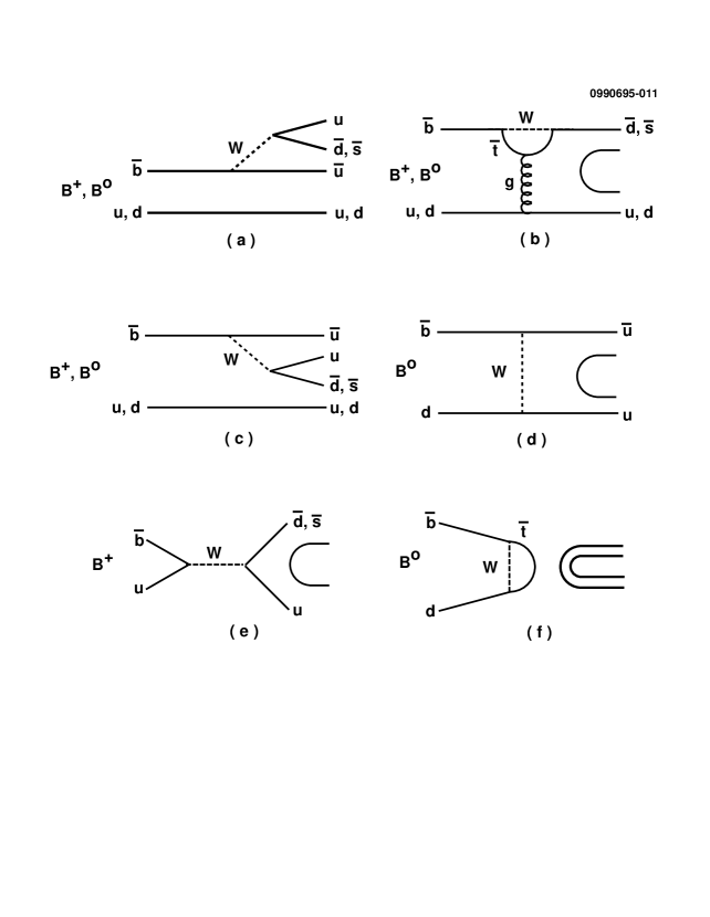
FIG. 1.: Feynman diagrams for rare hadronic $B$ decays: (a) $b\rightarrow u$ external $W$ emission, (b) $b\rightarrow s,d$ loop or gluonic penguin, (c) $b\rightarrow u$ internal $W$ emission, (d) $b\rightarrow u$ $W$ exchange, (e) annihilation, and (f) vertical $W$ loop.

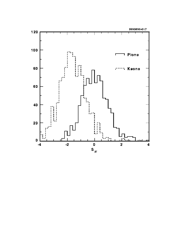
FIG. 2.: Distribution of $S_{\pi}$ for kinematically identified high momentum kaons and pions from $D^{*+}\rightarrow D^{0}\pi^{+};\ D^{0}\rightarrow K^{-}\pi^{+}$ decays. The solid line shows $S_{\pi}$ for pions and the dashed line shows $S_{\pi}$ for kaons.

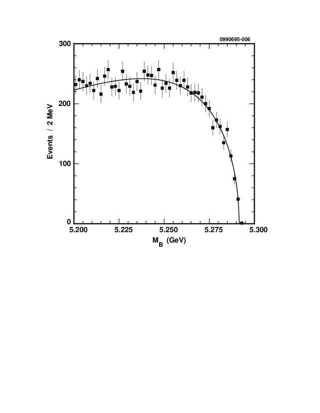
FIG. 3.: $M_{B}$ distribution from below-threshold background events (squares) and the fit to the parameterization given in the text (curve). The mass for the below-threshold data is shifted up to match the kinematic endpoint of the on-resonance data.

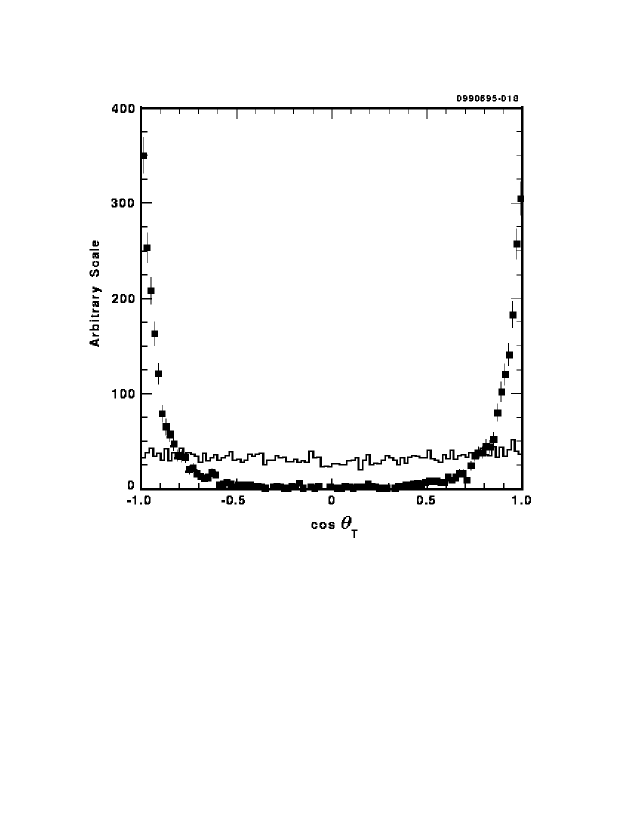
FIG. 4.: The $\cos\theta_{T}$ distributions for background data (squares) and $B^{0}\rightarrow\pi^{+}\pi^{-}$ Monte Carlo signal (histogram).

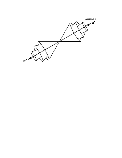
FIG. 5.: Illustration of the first three of the nine polar angle intervals.

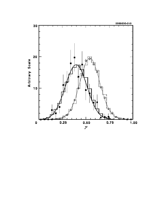
FIG. 6.: The $\cal F$ distribution for $B^{0}\rightarrow\pi^{+}\pi^{-}$ Monte Carlo (solid histogram), $B\rightarrow D\pi$ signal data (filled squares), the fit to the signal data (solid curve), the background Monte Carlo (dotted histogram), background data (open squares), and the fit to the background data (dotted curve).

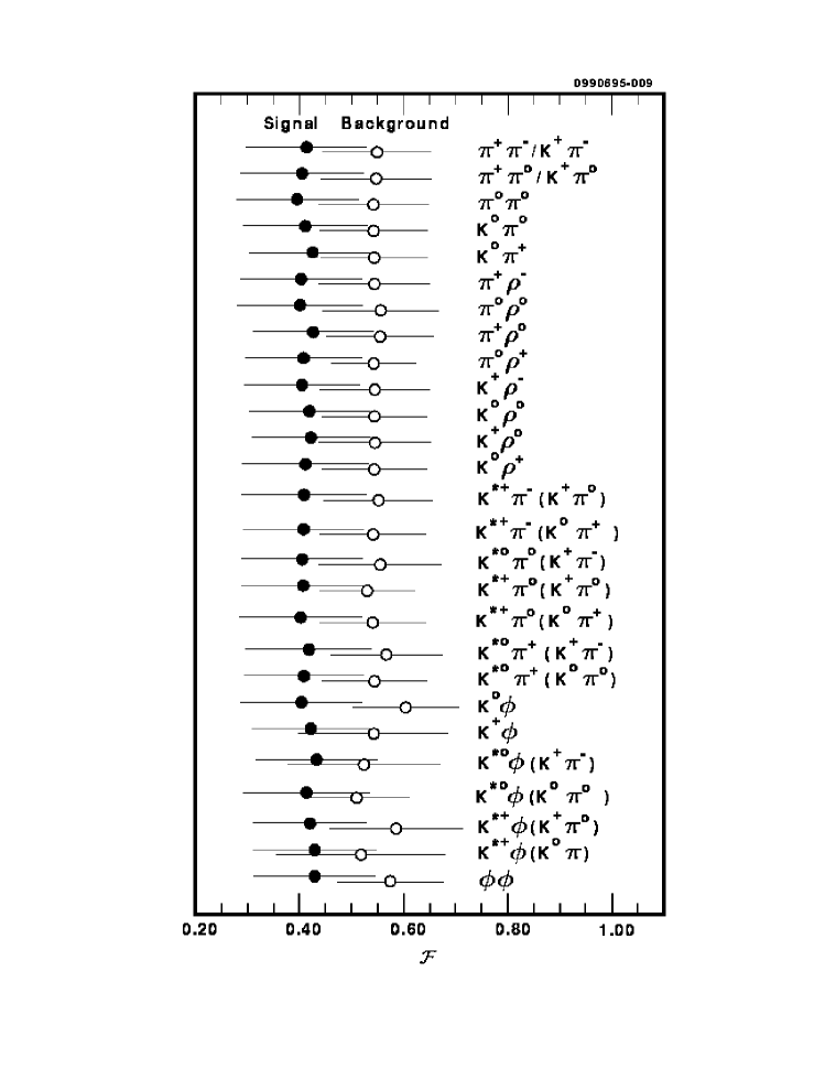
FIG. 7.: The means of the Fisher output distributions for signal (filled circles) and background (open circles) for the modes in this study. The error bars indicate the width of the distributions. Since the backgrounds in the $\phi$ modes are small, their background means are poorly measured.

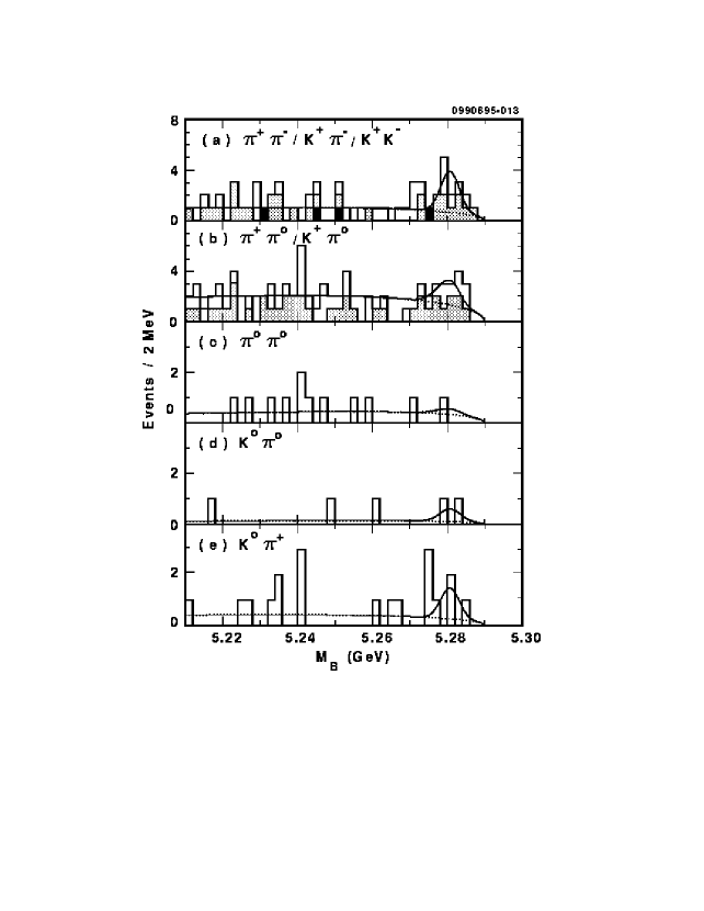
FIG. 8.: $M_{B}$ plots for (a) $B^{0}\rightarrow\pi^{+}\pi^{-}$ (unshaded) $B^{0}\rightarrow K^{+}\pi^{-}$ (grey), and $B^{0}\rightarrow K^{+}K^{-}$, (black) (b) $B^{+}\rightarrow\pi^{+}\pi^{0}$ (unshaded) and $B^{+}\rightarrow K^{+}\pi^{0}$ (grey), (c) $B^{0}\rightarrow\pi^{0}\pi^{0}$, (d) $B^{0}\rightarrow K^{0}\pi^{0}$, and e) $B\rightarrow K^{0}\pi^{+}$. The projection of the total likelihood fit (solid curve) and the continuum background component (dotted curve) are overlaid.

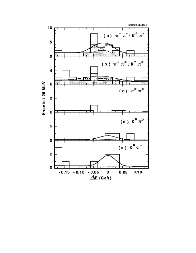
FIG. 9.: $\Delta E$ plots for (a) $B^{0}\rightarrow\pi^{+}\pi^{-}$ (unshaded) $B^{0}\rightarrow K^{+}\pi^{-}$ (grey), (b) $B^{+}\rightarrow\pi^{+}\pi^{0}$ (unshaded) and $B^{+}\rightarrow K^{+}\pi^{0}$ (grey), (c) $B^{0}\rightarrow\pi^{0}\pi^{0}$, (d) $B^{0}\rightarrow K^{0}\pi^{0}$, and (e) $B\rightarrow K^{0}\pi^{+}$. In plots (a) and (b), the projection of the total likelihood fit (upper solid curve), the $\pi\pi$ signal component (dotted curve), the $K\pi$ signal component (dashed curve), and the background component (lower solid curve) are overlaid. In plots (c)-(e), the total likelihood fit (solid curve) and background component (dotted curve) are overlaid.

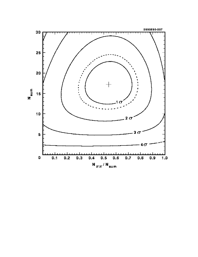
FIG. 10.: The central value ($+$) of the likelihood fit to $N_{\rm sum}\equiv N_{\pi\pi}+N_{K\pi}$ and $R\equiv N_{\pi\pi}/N_{\rm sum}$ for $B^{0}\rightarrow\pi^{+}\pi^{-}$ and $B^{0}\rightarrow K^{+}\pi^{-}$. The solid curves are the $n\sigma$ contours, and the dotted curve is the 1.28$\sigma$ contour.

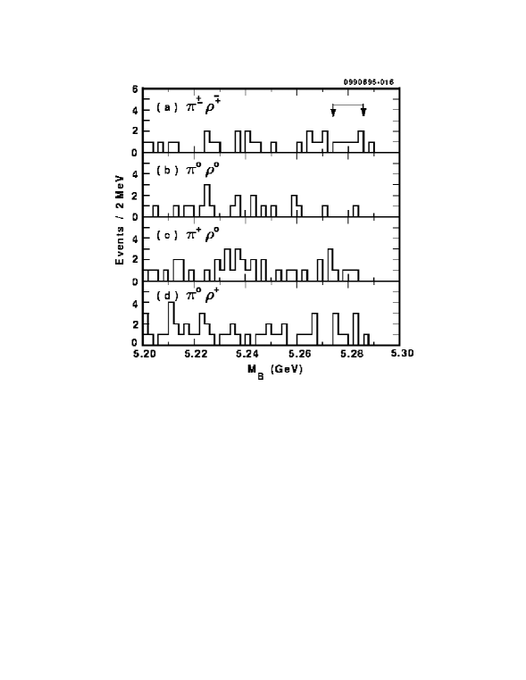
FIG. 11.: $M_{B}$ plots for (a) $B^{0}\rightarrow\pi^{\pm}\rho^{\mp}$, (b) $B^{0}\rightarrow\pi^{0}\rho^{0}$, (c) $B^{+}\rightarrow\pi^{+}\rho^{0}$, and (d) $B^{+}\rightarrow\pi^{0}\rho^{+}$. The signal region is indicated.

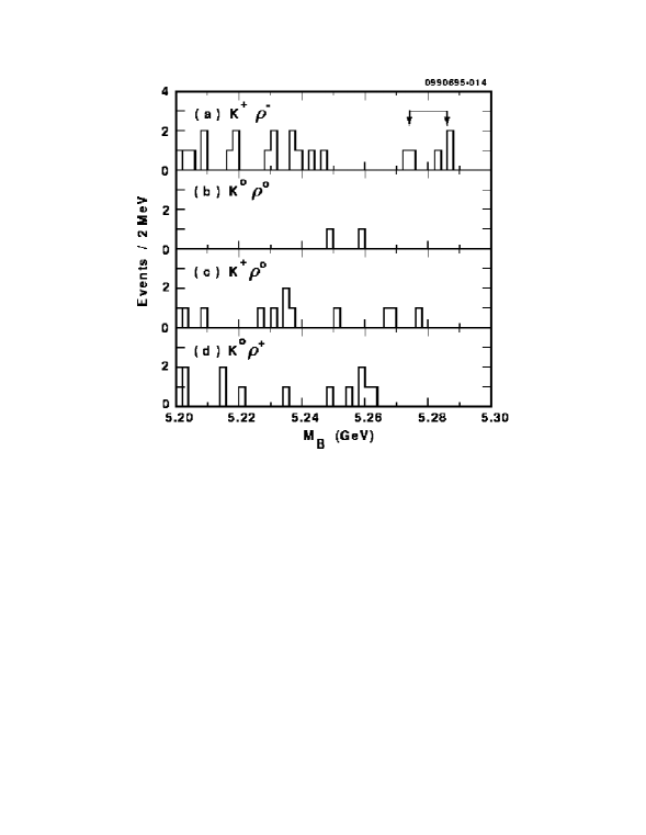
FIG. 12.: $M_{B}$ plots for (a) $B^{0}\rightarrow K^{+}\rho^{-}$, (b) $B^{0}\rightarrow K^{0}\rho^{0}$, (c) $B^{+}\rightarrow K^{+}\rho^{0}$, and (d) $B^{+}\rightarrow K^{0}\rho^{+}$. The signal region is indicated.

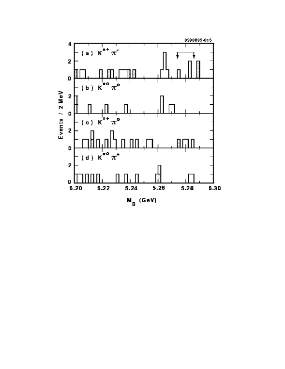
FIG. 13.: $M_{B}$ plots for (a) $B^{0}\rightarrow K^{*+}\pi^{-}$, (b) $B^{0}\rightarrow K^{*0}\pi^{0}$, (c) $B^{+}\rightarrow K^{*+}\pi^{0}$, and (d) $B^{+}\rightarrow K^{*0}\pi^{+}$. The shaded events are from $K^{*}\rightarrow K_{S}^{0}\pi$ decay modes and the unshaded events are from $K^{*}\rightarrow K^{+}\pi$ decay modes. The signal region is indicated.

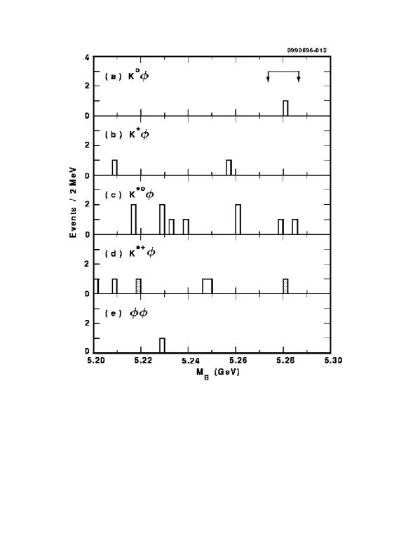
FIG. 14.: $M_{B}$ plots for (a) $B^{0}\rightarrow K^{0}\phi$, (b) $B^{+}\rightarrow K^{+}\phi$, (c) $B^{0}\rightarrow K^{*0}\phi$, (d) $B^{+}\rightarrow K^{*+}\phi$, and (e) $B^{0}\rightarrow\phi\phi$. The shaded events are from $K^{*}\rightarrow K_{S}^{0}\pi$ decay modes and the unshaded events are from $K^{*}\rightarrow K^{+}\pi$ decay modes. The signal region is indicated.