Neural Network based Electron Identification in the ZEUS Calorimeter

Abstract

We present an electron identification algorithm based on a neural network approach applied to the ZEUS uranium calorimeter. The study is motivated by the need to select deep inelastic, neutral current, electron proton interactions characterized by the presence of a scattered electron in the final state. The performance of the algorithm is compared to an electron identification method based on a classical probabilistic approach. By means of a principle component analysis the improvement in the performance is traced back to the number of variables used in the neural network approach.

DESY 95-054 ISSN 0418-9833

1 Introduction

One of the major scientific programs at the electron proton collider HERA is the study of deep inelastic electron proton scattering (DIS) in the so called low $x$ regime [1], where the constituents of the proton taking part in the interaction carry a very small fraction of its momentum. With its 27.5 GeV electron and a 820 GeV proton beams, HERA offers the unique opportunity to probe the proton structure down to $x=10^{-4}$ at typical scales, determined by the virtuality of the exchanged photon $Q^{2}$, of the order of $10$ GeV². The final state of these events is characterized by the presence of a scattered electron, at small angles relative to the initial direction of the electron beam, often accompanied by the fragmentation debris of the current jet. This makes the identification of the scattered electron a challenging task. In the ZEUS experiment [2], the main detector for these scattered electrons is the fine grained uranium scintillator calorimeter [3].

In the analysis presented in this paper the neural network approach is used for particle identification based on their showering properties in a segmented calorimeter. The aim is to best identify the electromagnetic particles using only the information from the uranium-scintillator calorimeter (CAL) of the ZEUS detector and to separate them from single hadrons or jets of particles for which the pattern of energy deposits in the CAL often looks quite similar especially at low energies.

In order to separate the signal from background by the pattern of energy deposits in the CAL, they should populate different regions in the multidimensional configuration space which is determined by the variables characterizing a pattern. In the classical approach to pattern recognition one usually tries to reduce the number of dimensions to a reasonable compromise, which allows to parameterize the correlations among the reduced variables without substantial loss of information. In case of the ZEUS calorimeter the electromagnetic showers can be described by up to 108 readout channels and the conventional electron finders reduce those to 2 - 7 variables at most. We propose the use of a neural network (NN) to find the optimal cuts in a multidimensional space in order to separate distinct distributions. In terms of a least square fit the NN adjusts the hyperplanes in the full configuration space in the course of which these hyperplanes replace the conventional low-dimensional cuts applied to the variables of the reduced configuration space. The neural network leads to hyperplanes which separate best the different distributions. This procedure ensures that all relevant information is used.

2 Physics motivation

The high center of mass energy (296 GeV) of the electron proton interactions at HERA extends the kinematic domain of lepton proton scattering to much higher momentum transfer ($Q^{2}\sim 5\cdot 10^{4}$ GeV²) and to much lower fractions of the proton momentum taking part in the hard interaction ($x\sim 10^{-4}$ for $Q^{2}\approx 10$ GeV²). Of particular interest is the so called low $x$ domain which is expected to shed some light on the transition between perturbative and non–perturbative phenomena of strong interactions and allow sensitive tests of QCD to be made in a regime dominated by QCD dynamics [1].

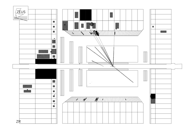
Figure 1: Event picture from the ZEUS detector showing a typical neutral current DIS event for $Q^{2}=310$ GeV².

The assignment of events to the various processes that can be studied at HERA is based on the identification of the properties of the final state. The signature of a deep inelastic neutral current interaction is the presence of an electron in the final state (see figure 1). Thus the major task of selecting deep inelastic events in data collection, reduction and classification relies on the ability to identify efficiently the final state electrons in a wide energy range. For low $x$ interactions the typical electron energy distribution extends from zero up to the kinematically allowed value, which in the case under study extends to about 30 GeV.

The large redundancy of information available in the ZEUS experiment for particle identification should provide a very high efficiency and high purity for electron identification. There are several experimental problems that make this task difficult. The asymmetry in the momenta of the colliding particles creates for the experiments at HERA problems typical for both low energy and high energy experiments. Particles scattered in the direction of the incoming electron, a configuration favored by the cross section, have low momenta. This configuration is typical for the low $x$ regime, where the final state electron is accompanied by the fragments of a low energy recoiling jet (see figure 2). As the particle energy decreases, it becomes harder to distinguish electron from pion showers based on the pattern of energy deposits in the calorimeter. This task is made even more difficult by the fact that particles are not isolated.

In the following we will discuss algorithms for electron identification which are optimized for the rear part of the ZEUS detector which integrates most of the low $x$ cross section. The analysis was performed on a large sample of Monte Carlo events passed through a full detector simulation and reconstruction.

3 Particle identification in the ZEUS calorimeter

ZEUS is a general purpose, magnetic detector with a tracking region surrounded by a high resolution calorimeter followed in turn by a backing calorimeter and a muon detection system. A detailed description of the ZEUS experiment can be found elsewhere [4].

The main component used for this study is the high resolution, uranium scintillator calorimeter (CAL) [3]. It is divided into three sections, the forward (FCAL), barrel (BCAL) and rear (RCAL) calorimeters. For normal incidence, the depth of the CAL is 7 interaction lengths in FCAL, 5 in BCAL and 4 in RCAL.

The relative thicknesses of uranium and scintillator in the layer structure were chosen to give equal calorimeter response to electrons and hadrons. Under test beam conditions, the energy resolution for electrons was measured [3, 5] to be $\sigma(E)/E=0.18/\sqrt{E}$ and for hadrons $\sigma(E)/E=0.35/\sqrt{E}$, where $E$ is in GeV.

Scintillator tiles form towers in depth that are read out on two sides through wavelength shifter bars, light guides and photomultipliers (PMTs). The towers are longitudinally segmented into electromagnetic (EMC) and hadronic (HAC) cells. The towers in FCAL and BCAL each have two HAC cells whereas those in RCAL have one. The depth of the EMC cells is 25 radiation lengths corresponding to one interaction length. Characteristic transverse sizes are 5 cm $\times$ 20 cm for the EMC cells of FCAL and BCAL and 10 cm $\times$ 20 cm for those in the RCAL. The HAC cells are typically 20 cm $\times$ 20 cm in the transverse dimension. The towers are read out by a total of 11836 PMTs.

The construction minimizes the possibility for particles from the interaction point (IP) to propagate down the boundaries between modules. Holes of 20 cm $\times$ 20 cm in the center of FCAL and RCAL are required to accommodate the HERA beam pipe. The resulting solid angle coverage is 99.7% of 4$\pi$.

Electron showers in the RCAL typically result in energy deposits above the noise suppression cut in three or four cells, with a tail to more cells due to interactions in the inactive material in front of the detector. Hadronic showers are generally much broader transversely and also much deeper longitudinally. On average, a $10$ GeV pion will leave energy above the noise suppression cut in 7 EMC cells and 6 HAC cells. There are large fluctuations from shower to shower depending primarily on the nature of the first few interactions, but in general electron pion separation improves with energy. For example, more than $50$ % of $1$ GeV pions entering the calorimeter will not leave any energy in the HAC, making it it very hard to distinguish them from electrons with the calorimeter alone, whereas less than $1$ % of $10$ GeV pions entering the calorimeter leave less than $2$ % of their energy in the HAC.

The noise in the calorimeter is dominated by the presence of the depleted uranium radioactivity. The noise levels range from $15$ MeV per cell in the EMC sections to $30$ MeV per cell in most HAC sections. Noise suppresion cuts of $60$ MeV and $110$ MeV are imposed in the EMC (HAC) respectively. On average 5 EMC cells and 2 HAC cells per event pass these cuts due to noise alone (from a total of 5918 cells).

4 Data selection

4.1 Monte Carlo Simulation

In order to reproduce fully the experimental conditions typical for deep inelastic neutral current interactions, events with $Q^{2}\geq 4$ GeV² were generated using a set of standard event generators which reproduce the event properties as measured in the ZEUS detector [6].

The detector acceptance and performance were simulated using the general purpose package GEANT [7]. The simulation incorporates our current knowledge of the experimental environment and trigger. The description of the responses of the various detector components was tuned to reproduce test data, the uranium calorimeter in particular [8]. The CAL noise was simulated according to the measured noise distributions. After full detector simulation the events were reconstructed with the standard ZEUS reconstruction program.

4.2 Clustering Algorithm

In a deep inelastic scattering process many particles and jets of particles from the interaction, including the final state electron, enter the geometrical acceptance of the CAL and deposit their energy in the calorimeter. The deposited energy is usually spread over several adjacent cells in the CAL. On average, one to two radiation length of inactive material are located between the interaction point and the surface of the CAL. This gives rise to preshowering effects in some fraction of the particles and increases the spread of the energy deposits.

The cluster algorithm used in this analysis was chosen such as to merge cells which belong most likely to the shower of a single particle. It is based on the idea of islands of energy, consisting of a bump of energy deposition surrounded by lower energy deposits. The smallest geometrical unit used in this particular application is a tower (described in section 3). Thus a cluster of adjacent towers can be subdivided into more clusters if groups of towers are separated by a distinct valley in the energy deposits. The principle of the island algorithm is depicted in figure 3. The energy in each tower of the CAL is compared to the energy of its neighbors. A tower becomes a seed for an island if all the neighboring towers have lower energy. Otherwise it is assigned a link to the neighboring tower with highest total energy deposition. All towers with links leading to the same seed are now assigned to one island.

For the further analysis the reconstructed clusters are classified. We denote a cluster as electromagnetic if it is generated by a single isolated electron or photon or by the scattered electron whether isolated or not. They will be denoted by $C_{e}$. All the remaining clusters whether corresponding to single hadrons or jets of particles are called hadronic clusters, $C_{h}$.

4.3 Preselection Cuts

Clusters corresponding to showers initiated by a single electromagnetic particle are expected to have most of their energy deposited in the EMC sections of the calorimeter and to be well contained transversely within a window of $3\times 3$ towers centered on the cluster tower with the highest energy deposition. A window of this size may also contain cells which were not assigned to the cluster. The latter are ignored in further analysis.

Electrons which enter the calorimeter close to the edge of the beam hole are likely to lose part of their energy in the beam hole or they may deposit substantial amounts of energy in the HAC sections. This class of clusters needs a special treatment and has been ignored in the present analysis. In order to reject those clusters, a crude position reconstruction was applied based on a linear energy weighting of cell centers belonging to a given cluster. This simple method is sufficient for our purpose. To exclude beam pipe clusters we reject those found within a square of $28\times 28$ cm² centered around the beam line.

In figure 4 we present for all reconstructed clusters the ratio of the energy deposited in the EMC sections of the window, $E^{W}_{EMC}$, to the total cluster energy contained in the window, $E^{W}_{tot}$. Whereas this ratio peaks at one for electrons and photons, it is evenly distributed between zero and one for hadrons. The lower values of $\frac{E^{W}_{EMC}}{E^{W}_{tot}}$ for the electromagnetic clusters are due to electrons which enter the calorimeter between two modules and deposit an unusual high fraction of their energy in the hadronic part of the calorimeter. No special study was made and they were removed from the sample by requiring ${~{}E^{W}_{EMC}~{}\over~{}E^{W}_{tot}~{}}>0.8\,$. This gives rise to a known inefficiency of the electron finder and leads to a loss of 1% of electrons while rejecting 84% of the hadronic clusters.

In figure 5 we present the ratio of $E^{W}_{tot}$ to $E^{C}_{tot}$, the total energy of the cluster as a function of $E^{C}_{tot}-E^{W}_{tot}$ for various classes of clusters as established at the generation level. For isolated electromagnetic particles the total energy of the cluster is indeed contained in the window as can be seen in figure 5a. In about 2% of the clusters corresponding to isolated electrons or photons the energy leakage of up to a few hundred MeV out of the window is caused by cells with random noise which pass the noise cut and thereby increase the size of the cluster.

In the low $x$ region the scattered electron is often accompanied by particles from the hadronic jet. As seen in figure 5b for non isolated electrons an increase of the energy leakage out of the window is observed. The effect is even more dramatic for hadronic clusters whose transverse size often exceeds that of $3\times 3$ towers (see figure 5c).

In order to enrich the sample in clusters which look like electromagnetic showers, we apply a set of preselection cuts to reject obvious non-electromagnetic clusters.

$$\frac{E^{W}_{EMC}}{E^{W}_{tot}}~{}>~{}0.8~{}~{}~{},~{}~{}~{}\frac{E^{W}_{tot}}{E^{C}_{tot}}~{}>~{}0.9~{}~{}~{},~{}~{}~{}E^{C}_{tot}-E^{W}_{tot}~{}<~{}1.0$$ (1)

Those cuts reject about 3% of electromagnetic clusters and 90% of hadronic clusters.

The energy distribution of the remaining electromagnetic and hadronic clusters is presented in figure 6. The largest overlap between the two classes of preselected clusters occur in the region of relatively low energies of the cluster. This is also the region where the separation of electromagnetic and hadronic showers is most difficult. In order to achieve the best efficiency and purity for electron identification we will limit the final sample used for tuning of electron finding to clusters of energy between 4 to 12 GeV. Above 12 GeV the separation of electromagnetic and hadronic showers is very good even with simple cuts. The properties of the hadronic clusters which pass our preselection cuts have a very weak energy dependence. This is not quite the case for the electromagnetic clusters as the lower energy end of the spectrum tends to be populated by electromagnetic showers which preshowered in the inactive material in front of the calorimeter. To increase the sensitivity of electron finders for low energy clusters we sample the spectrum of electromagnetic clusters to achieve a flat energy distribution in the final sample. We leave the hadronic spectrum unchanged.

In the range of 4 to 12 GeV, we generate two statistically independent samples each consisting of 3555 electromagnetic and 3555 hadronic clusters all of which passed our preselection cuts. The hadronic final state is a function of the fragmentation model used in the MC. We have chosen to work with an equal number of electromagnetic and hadronic clusters. The first sample, referred to as the training sample, serves to establish the cuts for the electron finders, while the second sample, the test sample, is used to check the performance of the finders. The efficiencies and purities which will be quoted further will refer to this specific mixture.

5 Electron Finders

As mentioned previously the purpose of this analysis was to built an electron finder optimized for identifying scattered electrons in the RCAL. To have a sufficient sample of low energy hadronic clusters we use the whole calorimeter. To achieve a single geometry for all clusters we reduce the information from the FCAL or the BCAL to the RCAL format as depicted in figure 7. In the EMC section we sum the signals from the two upper (lower) left and two upper (lower) right adjacent PMTs separately. We also sum separately the left and right PMTs of the HAC1 and HAC2 sections. The PMT signals are calibrated in GeV.

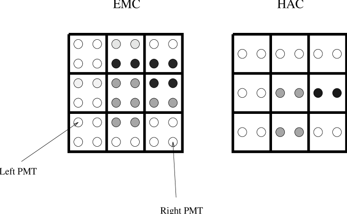
Figure 8: Schematic representation of the 54 energy deposits used as input for cluster identification. The various shadings shall indicate different energy deposits.

Each cluster which passed the preselection cuts is now characterized by 54 values of the energy deposits in the PMTs. Since the pattern of energy deposits depends on the angle of incidence of the particles, we include this angle $\delta$ as an additional input parameter. The angle of incidence $\delta$ is determined from the position of the cluster and the reconstructed vertex. Thus each candidate may be described by a set of 55 variables, the 54 energy deposits contained in the window (see figure 8) and $\cos\delta$.

The energy deposits in the CAL reflect the overall shape of the shower. As a consequence, it is hard to imagine that only one single variable of these 55 will enable one to distinguish between showers originating from electromagnetic or hadronic particles.

In search for the most discriminating properties of the showers we first apply the Principal Component Analysis (PCA) to the electromagnetic clusters [9]. Motivated by the results of the PCA, we apply then a classical probabilistic approach to electron finding. We choose two variables which are nonlinear combinations of the input variables and which describe both the longitudinal and transverse shape of the shower. Those are the radius of the shower and the fraction of the shower energy deposited in the electromagnetic section of the cluster. Finally, we apply the neural network approach to the training sample. The neural net uses all the 55 initial variables. We call the electron finder based on a classical probabilistic approach LOCAL, and the one based on the neural network approach SINISTRA.

5.1 Principal Component Analysis

The role of PCA is to establish a transformation of the input coordinate system into a system in which the transformed variables are ordered by the variance of their respective distributions. The ordering is such that the variables with the lowest variances have as low a variance as possible. PCA thus yields 55 linear combinations formed by eigenvectors and ordered in significance by their eigenvalues. The eigenvector with the largest eigenvalue provides the linear combination of the input variables which characterizes the pattern best. The eigenvalues (variances) obtained from PCA are presented in figure 9a. The transformation obtained from the PCA of the electromagnetic sample is then applied to the hadronic sample and the corresponding variances are plotted for comparison in figure 9a. The relative difference between the variances obtained from the two samples are plotted in figure 9b.

While from figure 9a one could conclude that two eigenvectors are of particular significance, the information contained in figure 9b suggests that for the separation of the two classes of clusters one needs more variables. A closer inspection of the eigenvectors shows that the first 10 eigenvectors mainly probe the electromagnetic structure of the cluster, while the rest probes the hadronic component as well.

5.2 Conventional Electron Finder – LOCAL.

To describe the shape of the showers we define two variables.

$$\epsilon~{}=~{}\frac{E^{W}_{EMC}}{E^{W}_{tot}}$$ (2)

and

$$r~{}=~{}\sqrt{~{}\sum\limits^{2}_{i=1}~{}\left[~{}\frac{\sum\limits_{Cells}E^{Cell}\cdot r^{2}_{i,Cell}}{E^{W}_{tot}}~{}-~{}\left(\frac{\sum\limits_{Cells}E^{Cell}\cdot r_{i,Cell}}{E^{W}_{tot}}\right)^{2}~{}\right]~{}}\ ,$$ (3)

where $E^{Cell}$ denotes the energy deposited in a cell located at position $(r_{1},r_{2})$ in the transverse plane and is equal to the sum of the energies obtained from the left and right PMTs.

The first variable $\epsilon$ is the fraction of energy deposited in the electromagnetic part of the calorimeter over the total energy of the cluster contained in the window. This parameter characterizes the longitudinal energy profile. The variable $r$ denotes an energy weighted radius of the shower describing its transverse spread. The sum extends only over cells contained within the window of $3\times 3$ towers. The distributions of $r$ for all electromagnetic and hadronic clusters are shown in figure 10. The distribution of $r$ for electromagnetic clusters with $\epsilon<1$ is shifted towards larger radii than that of clusters with $\epsilon=1$. The $r$ distribution of hadronic clusters is both shifted towards larger radii and broader than for electromagnetic clusters.

For the training sample we define the appropriate Bayesian probabilities which take into account the correlation between $r$ and $\epsilon$ for both hadronic and electromagnetic clusters. For a given cluster described by $r$ and $\epsilon$ we thus know the probability for it to be an electromagnetic cluster, $P(e|{\rm cluster})$. The resulting probability distribution of $P(e|{\rm cluster})$ for the test sample is presented in figure 11, for both the electromagnetic and hadronic showers. Hadronic clusters populate the region of low probabilities close to zero.

By varying the cut on the probability of a cluster to be electromagnetic, we can evaluate the integrated efficiency and integrated purity corresponding to this cut. The efficiency and purity are defined as follows :

$$\small{\rm efficiency} := \frac{N\left(~{}P(e|C_{e})>{\rm cut}~{}\right)}{N(\mbox{$C_{e}$})}$$ (4)

$${\rm purity} := \frac{N\left(~{}P(e|C_{e})>{\rm cut}~{}\right)}{N\left(~{}P(e|C_{e})>{\rm cut}~{}\right)~{}+~{}N\left(~{}P(e|C_{h})>{\rm cut}~{}\right)}~{}~{}~{},$$ (5)

where $N$ denotes the number of clusters passing the cuts described in the parenthesis and $N(\mbox{$C_{e}$})$ the total number of electromagnetic clusters. The efficiency as a function of purity is presented in figure 12, together with the results of the neural network electron finder that we describe below.

5.3 Neural Network Electron Finder – SINISTRA

A feedforward neural network can be regarded as a general tool to separate distinct distributions in a multidimensional space. In contrast to classical methods, which usually reduce the multidimensional space to several variables the neural network approach can be applied to the raw distributions. The reduction of the configuration space might lead to a loss of important information which may otherwise help to separate the distributions. Thus, for the neural network approach the complete manifold of available information is used.

The network is represented by a function, which connects in a non-linear way several transformation matrices. The entries of the matrices are denoted as weights and serve as the free parameters of the function. These weights are adjusted in terms of a least squares minimization of an error function. The neural network function is

$$\mbox{\boldmath$Y$}(\mbox{\boldmath$X$})=\tanh\left[~{}\frac{\mbox{$\cal A$}_{ij}~{}\tanh\left(~{}\frac{\mbox{$\cal B$}_{jk}X_{k}-\alpha_{j}}{t}~{}\right)-\beta_{i}}{t}~{}\right]$$ (6)

where $X_{k}$ denotes the $k$ component of the input vector $X$ of dimension $K$, $Y$ denotes the output vector of dimension $I$ and $i\>\epsilon\>[1,I]~{},~{}j\>\epsilon\>[1,J]~{}$ and $J$ is the number of hidden nodes. The matrices $\cal A$, $\cal B$, $\alpha$ and $\beta$ denote the weights and $t$ the temperature serving as a general smearing parameter. The Einstein convention for same indices is used.

We choose $I=1$ and thus the output of the neural network will be a scalar $Y$. Accordingly we define $O(C_{l})$ to be the desired output of the neural net, with $l\,\epsilon\,[e,h]$, depending on the class $C_{l}$ of the input pattern $X$

$$O(C_{l})~{}=~{}\left\{~{}\begin{array}[]{l}+1~{},~{}\mbox{if \mbox{\boldmath$X$} belongs to the class of electromagnetic clusters}~{}~{}(C_{e})\\ -1~{},~{}\mbox{if \mbox{\boldmath$X$} belongs to the class of hadronic clusters}~{}~{}(C_{h})\ ~{}~{}~{}~{}~{}~{}~{}~{}.\end{array}\right.$$

The cost function $E$ is defined as

$$E~{}=~{}\frac{1}{N}~{}\frac{1}{2}~{}\sum\limits_{n=1}^{N}~{}\left(~{}Y(\mbox{\boldmath$X$}(C_{l},n))~{}-~{}O(C_{l})~{}\right)^{2}~{}~{}~{},$$ (7)

where the sum runs over all $N=N(\mbox{$C_{e}$})+N(\mbox{$C_{h}$})$ patterns of the training sample. The training of the neural net consists of adjusting the weights in such a way, that for a pattern $X$ belonging to class $C_{e}$ the output $Y$ is close to $1$ and for hadronic cluster $C_{h}$ close to $-1$. In the training phase this error function is minimized by means of a gradient descent method yielding the appropriate changes for the weights and the temperature $t$. For the minimization of the error function $E$ we have chosen a method which is explained in detail in [10]. The main difference compared to the standard approach in the feedforward error back propagation neural networks is in that the matrices $\cal A$ and $\cal B$ are quadratically normalized to one for each row and the temperature $t$ acquires the meaning of a general smearing parameter. For high values of $t$ the error function $E$ depends only quadratically on the weights. Thus for this regime of $t$, $E$ exhibits only one minimum. It is expected that further decrease of $t$ leads to the global minimum of the error function. The temperature is treated as another free parameter whose value is changed in terms of a gradient descent method.

The approach to the global minimum of the error function (7) is monitored by the development of the temperature $t$ and the percentage of misidentification as functions of the iteration step, denoted as epoch. The percentage of misidentification is defined as

$$\small f~{}:=~{}\frac{N\left(~{}P(e|C_{e})<0.5~{}\right)~{}+~{}N\left(~{}P(e|C_{h})>0.5~{}\right)}{N(\mbox{$C_{e}$})~{}+~{}N(\mbox{$C_{h}$})}~{}~{}~{},$$ (8)

where $N(\mbox{$C_{h}$})$ denotes the total number of hadronic clusters. Initially the entries of the weights are chosen at random in some interval around zero. Therefore the values for the temperature $t$ and $f$ depend in the beginning on these initial conditions. It is expected, that when the minimization procedure approaches the global minimum of the error function $E$, the values of $t$ and $f$ become independent of the initial values chosen for the weights. Close to the global minimum the temperature tends to a value which depends on the inherent overlap in the configuration space of classes $C_{e}$ and $C_{h}$ [10] and thus on $E$. The values of $t$ and $E$ at the global minimum (denoted by gm) are approximately related to each other by

$$E^{\rm gm}~{}\approx~{}\frac{t^{{\rm gm}}}{1+t^{{\rm gm}}}~{}.$$ (9)

In figure 13 we present the mean and the rms spread $(\sigma)$ of $t$ and $f$ for 10 different initial conditions as functions of the epoch, where all 55 entries of the general input had been used. Initially we observe a dispersion of about 5 % for $f$ which after about 50 epochs becomes negligible. The dispersion of $t$ is negligible throughout the whole training phase.

The value of the cost function $E$ (7) depends on the patterns of the training sample and on the architecture of the neural network function $Y(\mbox{\boldmath$X$})$. In order to avoid overtraining of the net we use the test sample to check whether the network is not biased towards the training sample. The correlation between the mean $f^{train}$ and $f^{test}$ are plotted for each epoch in figure 14. Although after about 1000 epochs we observe an indication of overtraining, both the errors for the training sample and the test sample still decrease. The difference between the errors remains well within the statistical error of each of the samples. The minimization procedure is stopped after 2000 epochs.

The effect of the minimization procedure on the number of hidden nodes (i.e. the value of $J$) has been studied. The studies have shown that 4 hidden nodes were sufficient and more hidden nodes did not improve the performance. Therefore all further results are obtained with $J\,=\,4$.

It can be shown that a squared error cost function is minimized when network outputs are minimum, mean-squared, error estimates of Bayesian probabilities [11]. Thus the output value $Y$ as defined in equation (6) can be related to an estimator for the a posteriori Bayesian probability, $P(e|{\rm cluster})$,

$$P(e|{\rm cluster})~{}=~{}0.5\times(~{}1+Y~{})~{}~{}~{}.$$ (10)

The resulting probability distribution, $P(e|{\rm cluster})$, of the test sample is presented in figure 15 where the separate contribution of $C_{e}$ and $C_{h}$ are also indicated. As expected the probability for the electromagnetic clusters is close to 1, while that for hadronic clusters is close to 0. A cut on the probability leads to a separation of electromagnetic and hadronic clusters with a certain purity and efficiency. This is shown in figure 12.

5.4 Comparison of the different methods

In figure 12 we presented the efficiency versus purity curves obtained with LOCAL and SINISTRA. In both cases the variation is obtained by changing the cut on the probability which determines whether the cluster is electromagnetic or hadronic. Clearly the neural network electron finder performs better than the conventional one. For a given purity the efficiency of the neural network is higher than for the conventional finder built with two variables.

In order to understand the difference in performance we studied the separation power depending on the number of input dimensions. For that purpose we used as input variables the results of the PCA, in decreasing order of significance for the electromagnetic clusters. For a given set of variables we repeated the neural network approach and generated an efficiency versus purity curve. In figure 16 we present the purity as a function of the number of input variables for a fixed efficiency of 85%. With the increase of the number of variables we observe an increase of purity. The pattern in the improvement is correlated to the relative difference in the eigenvalues described in section (5.1) and their significance. The biggest increase in purity is registered when the input variables start to include the information on the hadronic component of the clusters as established by inspecting the corresponding eigenvectors. The lack of improvement after about 34 PCA variables is probably due to the smallness of their variances and due to numerical limitations as the network cannot resolve the differences.

Since the 34 PCA variables use all 55 initial input values this analysis indicates, that all 55 input values contain information which is useful to separate electromagnetic from hadronic showers in the CAL. Leaving out information results in a deterioration of the performance. On the other hand for an efficiency of 85% the purity of LOCAL is higher than the purity achieved with 17 PCA variables. Thus a smaller number of non-linear combinations of several variables might yield an equivalent performance as a larger set of linearly transformed variables. Thus in the case under study the improvement in the performance of the neural network electron finder over the conventional one is primarily due to the number of variables which are used for the separation of patterns.

6 Conclusions

In this paper we have presented a comparison between the performance of a conventional electron finder based on two variables and a neural network using the full manifold of available information provided by the segmented uranium calorimeter of the ZEUS detector. The analysis was carried on samples of events produced by a detailed Monte Carlo simulation of the deep inelastic electron proton interactions and of the experimental environment of the ZEUS detector. The neural network uses 54 energy deposits registered in an area of $60\times 60$ cm² in the electromagnetic and the hadronic sections of the calorimeter and the cosine of the angle of incidence. For the conventional electron finder the 54 energy deposits are transformed into the energy weighted radius for the transverse spread of the shower and the ratio of the energy deposited in the electromagnetic section of the calorimeter to the total energy to describe its longitudinal shape. We find that for a given efficiency of electron identification the purity of the neural network electron finder is larger than for the conventional one. A principle component analysis (PCA) of the 55 input variables describing an electromagnetic cluster allows to establish that the improvement is due to the number of variables used for the classification. It also shows that the conventional electron finder with two non-linear combinations of the 54 energy deposits is as powerful as a neural network classifier based on the 17 most significant linear combinations of the PCA analysis.

Acknowledgments

This work has been pursued in the framework of the ZEUS collaboration and we would like to acknowledge the motivating interest of our colleagues. We would also like to thank the DESY directorate for its hospitality. We are indebted to Prof. David Horn for his many helpful suggestions on the application of neural networks.

Figure 2: Schematic representation of the opening angle in the LAB frame between the scattered electron (thin arrows) and the struck quark (bold arrows) for various points in the $Q^{2}-x$ plane. The length of the arrows are scaled relative to the initial energy of the incoming electron.

Figure 3: Schematic representation of Islands clustering. A dot represents a seed and the towers assigned to a cluster are represented by the arrows pointing towards the seed.

Figure 4: Distribution of the fraction of the total energy $(~{}E^{W}_{tot}~{})$ deposited in the EMC sections for electromagnetic and hadronic clusters.

Figure 5: Ratio of the total energy of a cluster contained in the window $(E^{W}_{tot})$ over the total energy of this cluster $(E^{C}_{tot})$ plotted as a function of the difference between the two energies. (Note that in figure a) 98% of all entries are represented by one point at $E^{W}_{tot}/E^{C}_{tot}=1$ and $E^{C}_{tot}-E^{W}_{tot}=0$.)

Figure 6: Spectrum of electromagnetic and hadronic clusters after some coarse preselection cuts had been applied.

Figure 7: Schematic representation of the way the FCAL and BCAL granularity is reduced to match that of the RCAL.

Figure 9: a) Eigenvalues, Var, (dots) of the transformation matrix obtained by the principle component analysis of the electromagnetic clusters as a function of the eigenvector number, compared to the appropriate variances of the sample of hadronic clusters (squares). b) The relative difference in the variances, $\Delta$ between the electromagnetic and hadronic clusters as a function of the eigenvector number.

Figure 10: Distribution of the energy weighted radius $r$ for a) electromagnetic clusters with $\epsilon\,=\,1$, b) electromagnetic clusters with $\epsilon\,<\,1$ and c) for hadronic clusters

Figure 11: Probability distribution for a given cluster to be an electromagnetic cluster $P(e~{}|~{}{\rm cluster})$ using the LOCAL electron finder.

Figure 12: Efficiency versus purity for electron identification as obtained for the electron finder LOCAL (based on two non-linear variables) and SINISTRA (neural network based on 55 variables).

Figure 13: The average temperature and the average percentage of misidentification $f^{train}$ as a function of the epoch, for 10 different sets of initial weights. The error bars correspond to the RMS of the 10 samples for each epoch.

Figure 14: The $f^{train}$ versus $f^{test}$ for each epoch. The values of $f^{train}$ and $f^{test}$ were obtained by averaging over 10 sets with different initial weights. The lines of $\pm~{}1\sigma$ correspond to variations allowed by the statistical error of the train and test sample.

Figure 15: Probability distribution for a given cluster to be an electromagnetic cluster $P(e~{}|~{}{\rm cluster})$ using the SINISTRA electron finder.

Figure 16: Purity as a function of the number of input variables for a fixed efficiency of 85%.

References

- [1] W. Buchmüller and G. Ingelman, editors. Proc. HERA workshop, Vol. 1, Hamburg, 1991.
- [2] ZEUS Collaboration. The ZEUS detector, status report. DESY PRC 93-05, 1993.
- [3] M. Derrick et al. Nucl. Inst. Meth. A, 309:77, 1991.
- [4] ZEUS Collaboration; M. Derrick et al. A measurement of sigma/tot (gamma proton) at sqrt(s)=210 GeV. Phys. Lett. B, 293:465–477, 1992.
- [5] A. Andresen et al. Nucl. Inst. Meth. A, 309:101, 1991.
- [6] ZEUS Collaboration; M. Derrick et al. Measurement of the proton structure function from the 1993 HERA data. DESY 94-143, 1994.
- [7] R. Brun et al. Geant 3. CERN/DD/EE/84-1, 1987.
- [8] Yoshihisa Iga. Simulation of the ZEUS calorimeter. DESY 95-005, 1995.
- [9] H. Wind. Principle component analysis and its application to track finding. In Formulae and Methods in Experimental Data Evaluation, volume 3, pages K1–K16. R.K. Bock, 1984.
- [10] R. Sinkus. A novel approach to error function minimization for feedforward neural networks. DESY 94-182, 1994.
- [11] Michael D. Richard and Richard P. Lippmann. Neural network classifiers estimate bayesian a posteriori probabilities. Neural Computation, 3:461–483, 1991.